$SU(3)$ Quantum Spin Ladders as a Regularization of the ${\mathbb{C}P}(2)$ Model at Non-Zero Density:
From Classical to Quantum Simulation

Abstract

Quantum simulations would be highly desirable in order to investigate the finite density physics of QCD. $(1+1)$-d ${\mathbb{C}P}(N-1)$ quantum field theories are toy models that share many important features of QCD: they are asymptotically free, have a non-perturbatively generated massgap, as well as $\theta$-vacua. $SU(N)$ quantum spin ladders provide an unconventional regularization of ${\mathbb{C}P}(N-1)$ models that is well-suited for quantum simulation with ultracold alkaline-earth atoms in an optical lattice. In order to validate future quantum simulation experiments of ${\mathbb{C}P}(2)$ models at finite density, here we use quantum Monte Carlo simulations on classical computers to investigate $SU(3)$ quantum spin ladders at non-zero chemical potential. This reveals a rich phase structure, with single- or double-species Bose-Einstein “condensates”, with or without ferromagnetic order.

1 Introduction

Monte Carlo simulations of Wilson’s lattice QCD [1] are very successful in addressing static properties of hadrons [2, 3] as well as the equilibrium thermodynamics of quarks and gluons at zero baryon density [4, 5]. The real-time dynamics and the non-zero density physics of QCD [6], on the other hand, remain largely unexplored, because Monte Carlo simulations then suffer from very severe sign and complex action problems. Quantum simulation experiments are very promising for addressing these challenging questions, because quantum hardware (whose dynamics naturally incorporates quantum entanglement) does not suffer from such problems [7, 8, 9, 10, 11, 12]. Indeed, quantum simulation experiments have already been carried out successfully in the context of condensed matter physics. In particular, the real-time evolution through a quantum phase transition in the bosonic Hubbard model, which separates a Mott insulator from a superfluid, has been realized in quantum simulation experiments with ultracold bosonic atoms in an optical lattice [13]. Similar experiments with fermionic atoms aim at quantum simulations of the fermionic Hubbard model, in the context of high-temperature superconductivity. The current experiments with fermionic gases have not yet succeeded to reach sufficiently low temperatures to explore the possible existence of high-temperature superconductivity in the fermionic Hubbard model. However, medium-range antiferromagnetic correlations have already been observed [14].

These impressive developments in the quantum simulation of condensed matter systems provide a strong motivation to explore the feasibility of quantum simulation experiments of QCD and other quantum field theories relevant in particle physics. While it seems difficult to embody Wilson’s lattice QCD in ultracold quantum matter, an attractive alternative lattice regularization of QCD and other asymptotically free field theories is provided by quantum link models [15, 16, 17, 18, 19]. Quantum links are generalized quantum spins (associated with the links of a lattice) with an exact gauge symmetry. Wilson’s link variables are classical $SU(3)$-valued parallel transporter matrices with an infinite-dimensional link Hilbert space. $SU(3)$ quantum links are again $3\times 3$ matrices, but their matrix elements are non-commuting operators that act in a finite-dimensional link Hilbert space. This makes quantum link models ideally suited for quantum simulation experiments in which a finite number of quantum states of ultracold matter can be controlled successfully [20]. Indeed, quantum simulation experiments of Abelian [21, 22, 23, 24] and non-Abelian gauge theories [25, 26, 27], some based on quantum link models have already been proposed. In particular, ultracold alkaline-earth atoms in an optical superlattice [27] are natural physical objects that can embody non-Abelian $U(N)$ and $SU(N)$ gauge theories.

While first quantum simulation experiments of relatively simple Abelian and non-Abelian lattice gauge theories are expected in the near future, the quantum simulation of QCD remains a long-term goal [28]. The quantum link regularization of QCD [18] involves an additional spatial dimension (of short physical extent) in which the discrete quantum link variables form emergent continuous gluon fields via dimensional reduction. The extra dimension also gives rise to naturally light domain wall quarks with an emergent chiral symmetry. Incorporating these important dynamical features in quantum simulation experiments will be challenging, but does not seem impossible. In particular, synthetic extra dimensions have already been realized in quantum simulation experiments with alkaline-earth atoms [29].

In order to explore the feasibility of quantum simulation experiments of QCD-like theories, it is natural to investigate $(1+1)$-d ${\mathbb{C}P}(N-1)$ models [30, 31]. These quantum field theories share crucial features with QCD: they are asymptotically free, have a non-perturbatively generated massgap, as well as non-trivial topology and hence $\theta$-vacuum states. In particular, the ${\mathbb{C}P}(N-1)$ model has a global $SU(N)$ symmetry that gives rise to interesting physics at non-zero density, which can be explored via chemical potentials. As in QCD, the direct classical simulation of ${\mathbb{C}P}(N-1)$ model $\theta$-vacua, finite density physics, or dynamics in real-time suffer from severe sign problems, and thus strongly motivate the need for quantum simulation. Again, alkaline-earth atoms in an optical superlattice are natural degrees of freedom to realize the $SU(N)$ symmetry of ${\mathbb{C}P}(N-1)$ models [32, 33].

In complete analogy to the quantum link regularization of QCD, $(1+1)$-d ${\mathbb{C}P}(N-1)$ models can be regularized using $(2+1)$-d $SU(N)$ quantum spin ladders [37, 38]. Again, there is an extra spatial dimension of short physical extent in which the discrete quantum spins form emergent continuous ${\mathbb{C}P}(N-1)$ fields via dimensional reduction. The continuum limit of the $(1+1)$-d ${\mathbb{C}P}(N-1)$ quantum field theory is taken by gradually increasing the extent $L^{\prime}$ of the extra dimension. Thanks to asymptotic freedom, this leads to an exponential increase of the correlation length $\xi\gg L^{\prime}$ in the physical dimension, and thus to dimensional reduction from $(2+1)$-d to $(1+1)$-d, similar to the $O(3)={\mathbb{C}P}(1)$ model [39, 40]. All this is analogous to QCD, but has the great advantage that it can already be investigated with currently available experimental quantum simulation techniques. In particular, by varying $L^{\prime}$ it should be possible to approach the continuum limit of the $(1+1)$-d ${\mathbb{C}P}(N-1)$ quantum field theory in ultracold atom experiments.

In order to validate and support upcoming quantum simulation experiments of ${\mathbb{C}P}(N-1)$ models at zero and non-zero density, here we use quantum Monte Carlo calculations (on classical computers) to simulate $SU(N)$ quantum spin ladders with chemical potential. This method was first used in [41] to investigate the $(1+1)$-d $O(3)={\mathbb{C}P}(1)$ model at non-zero chemical potential using a meron-cluster algorithm. Here we focus on the $N=3$ case of the ${\mathbb{C}P}(2)$ model with a global $SU(3)$ symmetry [42] which is accessible to quantum simulation experiments. Since $SU(3)$ has rank 2, with two commuting generators $T^{3}$ and $T^{8}$, there are two independent chemical potentials $\mu_{3}$ and $\mu_{8}$. A chemical potential $\mu_{3}\neq 0$ generically breaks the global $SU(3)$ symmetry explicitly down to $U(1)_{3}\times U(1)_{8}$. As we will show, at zero temperature the $U(1)_{3}$ symmetry undergoes the Kosterlitz-Thouless phenomenon and the remaining symmetry is reduced to $U(1)_{8}$. Due to the Mermin-Wagner theorem, this is as close as a $(1+1)$-d quantum field theory can come to Bose-Einstein “condensation”. Interestingly, for $\mu_{3}=0$ and $\mu_{8}\neq 0$, the $SU(3)$ symmetry is explicitly broken only to $SU(2)_{123}\times U(1)_{8}$. Now the $U(1)_{8}$ symmetry undergoes the Kosterlitz-Thouless phenomenon. The $SU(2)_{123}$ symmetry then gives rise to a double-species Bose-Einstein “condensate”. The $SU(2)_{123}$ “spin” $(T^{1},T^{2},T^{3})$ is a conserved order parameter, just like the total spin of a ferromagnetic quantum spin chain. Remarkably, we thus obtain a double-species “ferromagnetic” Bose-Einstein “condensate”. It will be most exciting to explore this rich phase structure of the $(1+1)$-d ${\mathbb{C}P}(2)$ model with experimental quantum simulations of alkaline-earth atoms in an optical lattice. Our classical simulations can serve as a valuable tool to validate future experiments of this kind.

The rest of the paper is organized as follows. In Section 2 we introduce $(2+1)$-d $SU(N)$ quantum spin ladders as a regularization of $(1+1)$-d ${\mathbb{C}P}(N-1)$ models. In particular, we discuss the mechanism of dimensional reduction from $(2+1)$-d to $(1+1)$-d. In Section 3 we focus on $(2+1)$-d $SU(3)$ quantum spin ladders and the resulting $(1+1)$-d ${\mathbb{C}P}(2)$ model, with a special emphasis on its finite-density physics. We present results of quantum Monte Carlo calculations to explore the phase diagram and to investigate the nature of the various phases. We also measure various correlation functions in order to investigate the properties of the excitations in different regions of the phase diagram. Finally, Section 4 contains our conclusions. The details of a quantum Monte Carlo worm algorithm are described in an appendix.

2 From $SU(N)$ Quantum Spin Ladders to
${\mathbb{C}P}(N-1)$ Models

In this section, we introduce an antiferromagnetic $SU(N)$ quantum spin ladder and discuss its low-energy effective field theory, which leads to the ${\mathbb{C}P}(N-1)$ model via dimensional reduction.

2.1 Antiferromagnetic $SU(N)$ Quantum Spin Ladder

Figure 1: Spin ladder of length $L$ in the 1-direction, consisting of $n=L^{\prime}/a$ transversely coupled spin chains. The even sites on sublattice $A$ (open circles) carry an $SU(N)$ quantum spin in the fundamental $\{N\}$ representation, while the odd sites on sublattice $B$ (filled circles) carry the anti-fundamental $\{\overline{N}\}$ representation. Periodic and open boundary conditions are imposed in the 1- and 2-direction, respectively.

Let us consider a 2-d bipartite square lattice of large extent $L$ in the periodic 1-direction and short extent $L^{\prime}$ in the 2-direction with open boundary conditions. In the continuum limit, the 2-direction will ultimately disappear via dimensional reduction, while the 1-direction remains as the physical spatial dimension [37]. As illustrated in Fig.1, we distinguish the sites $x\in A$ of the even sublattice $A$ from the neighboring sites $y\in B$ of the odd sublattice $B$. We place $SU(N)$ quantum spins $T^{a}_{x}=\frac{\lambda^{a}}{2}$ in the fundamental representation $\{N\}$ on sublattice $A$. Here $\lambda^{a}$ (with $a\in\{1,2,\dots,N^{2}-1\}$) are the generators of the $SU(N)$ algebra; for $N=3$ they are the Gell-Mann matrices. As a consequence, the spins obey the commutation relations

$$[T_{x}^{a},T_{x^{\prime}}^{b}]=i\delta_{xx^{\prime}}f_{abc}T_{x}^{c}\ ,$$ (2.1)

with the structure constants $f_{abc}$ of the $SU(N)$ algebra. For $N=3$ it is useful to introduce the shift operators

$$T^{\pm}=T^{1}\pm iT^{2},\quad V^{\pm}=T^{4}\pm iT^{5},\quad U^{\pm}=T^{6}\pm iT^{7}\ .$$ (2.2)

On sublattice $B$, on the other hand, we place quantum spins $\overline{T}^{a}_{y}=-\frac{{\lambda^{a}}^{*}}{2}$ in the complex conjugate anti-fundamental representation $\{\overline{N}\}$, which again obey

$$[\overline{T}_{y}^{a},\overline{T}_{y^{\prime}}^{b}]=i\delta_{yy^{\prime}}f_{abc}\overline{T}_{y}^{c}\ ,$$ (2.3)

For $SU(3)$ the weight diagrams of the fundamental and anti-fundamental representations $\{3\}$ and $\{\overline{3}\}$ are illustrated in Fig.2.

An antiferromagnetic $SU(N)$ quantum spin ladder (with $J>0$) is then described by the nearest-neighbor Hamiltonian

$$H=J\sum_{\langle xy\rangle}T^{a}_{x}\overline{T}^{a}_{y}\ ,$$ (2.4)

which commutes with the total $SU(N)$ spin

$$T^{a}=\sum_{x\in A}T^{a}_{x}+\sum_{y\in B}\overline{T}^{a}_{y}\ ,$$ (2.5)

i.e. $[H,T^{a}]=0$.

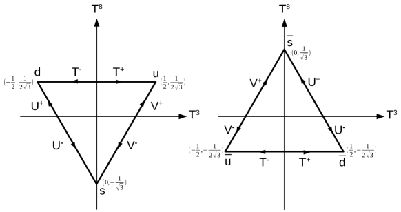
Figure 2: Fundamental $SU(3)$ triplet representation $\{3\}$ (left) and anti-fundamental representation $\{\overline{3}\}$ (right). The shift operators $T^{\pm}$, $U^{\pm}$, and $V^{\pm}$ (cf. eq.(2.2)) relate the different states of the multiplets.

Let us also couple a chemical potential $\mu_{a}$ to the conserved non-Abelian $SU(N)$ charge $T^{a}$ by subtracting a term $\mu_{a}T^{a}$ from the Hamiltonian. For $N=3$, such a term can always be diagonalized to $\mu_{3}T^{3}+\mu_{8}T^{8}$ by a unitary transformation, with two independent chemical potentials $\mu_{3}$ and $\mu_{8}$. The grand canonical partition function (at inverse temperature $\beta$) then takes the form

$$Z=\mbox{Tr}\exp(-\beta(H-\mu_{a}T^{a}))\ .$$ (2.6)

Let us first consider the $SU(N)$ spin system at zero temperature, $\beta\rightarrow\infty$, in the infinite-volume limit, $L,L^{\prime}\rightarrow\infty$. For $N\leq 4$ the system then breaks its $SU(N)$ symmetry down to $U(N-1)$ [43]. This generalizes the $SU(2)\rightarrow U(1)$ symmetry breaking of the antiferromagnetic Heisenberg model to $SU(3)$ and $SU(4)$ quantum spin systems. For $N\geq 5$, on the other hand, the simple Hamiltonian of eq.(2.4) gives rise to a dimerized state with spontaneously broken lattice translation symmetry [43]. One can easily imagine that more complicated Hamiltonians would still support spontaneous $SU(N)\rightarrow U(N-1)$ breaking even for $N\geq 5$, which is what we will assume when we discuss general $N$. Later, we will focus our attention on the $N=3$ case, in which the simple Hamiltonian of eq.(2.4) gives rise to spontaneous $SU(3)\rightarrow U(2)$ symmetry breaking.

2.2 The $(2+1)$-d ${\mathbb{C}P}(N-1)$ Model as a Low-Energy Effective Field Theory

When a global $G=SU(N)$ symmetry breaks spontaneously to an $H=U(N-1)$ subgroup, $N^{2}-1-(N-1)^{2}=2N$ massless Goldstone bosons arise. Their low-energy dynamics are described by an effective field theory in terms of Goldstone boson fields $P(x)$ which take values in the coset space $G/H=SU(N)/U(N-1)={\mathbb{C}P}(N-1)$. Here $x$ is a point in the $(2+1)$-d Euclidean space-time continuum and $P(x)$ is an $N\times N$ matrix-valued field that obeys

$$P(x)^{\dagger}=P(x),\quad P(x)^{2}=P(x),\quad\mbox{Tr}P(x)=1\ ,$$ (2.7)

i.e. $P(x)$ is a Hermitean projection operator. The field $P(x)$ can be diagonalized by a unitary transformation $U(x)\in SU(N)$ such that

$$U(x)P(x)U(x)^{\dagger}=\mbox{diag}(1,0,\dots,0)\ .$$ (2.8)

Since $P(x)$ is a projection operator with trace 1, the resulting diagonal matrix has one entry 1 and $N-1$ entries 0. This matrix commutes with all $U(N-1)=SU(N-1)\times U(1)$ matrices. Consequently, $P(x)$ is affected only by those $SU(N)$ matrices $U(x)$ that belong to the coset space $SU(N)/U(N-1)={\mathbb{C}P}(N-1)$. Global symmetry transformations $\Omega\in SU(N)$, which manifest themselves as

$$P(x)^{\prime}=\Omega P(x)\Omega^{\dagger}\ ,$$ (2.9)

indeed leave the defining relations of eq.(2.7) invariant.

The action of the low-energy effective theory contains all terms that respect all symmetries of the underlying microscopic Hamiltonian of eq.(2.4), in particular, the global $SU(N)$ symmetry. The leading term in a systematic low-energy expansion has only two derivatives and gives rise to the effective action

$$S[P]=\int d^{3}x\frac{\rho_{s}}{c}\mbox{Tr}\left[\partial_{\mu}P\partial_{\mu}P\right]\ .$$ (2.10)

Here $\rho_{s}$ is the spin stiffness, $c$ is the spinwave velocity, and $x_{3}=ct$ is the appropriately rescaled Euclidean time coordinate. Note that we put $\hbar$ (but not $c$) to 1.

2.3 Dimensional Reduction to the $(1+1)$-d ${\mathbb{C}P}(N-1)$ Model

As long as we stay in the infinite-volume limit of the $(2+1)$-d Euclidean space-time volume, the action from above describes strictly massless Goldstone bosons. As soon as we deviate from this limit, for example, by making the extent $L^{\prime}$ of the 2-direction finite, the Mermin-Wagner theorem implies that the continuous global $SU(N)$ symmetry can no longer break spontaneously. As a consequence, the Goldstone bosons pick up an exponentially small mass [39, 40, 37]. Interestingly, this non-perturbative effect is still captured by the Goldstone boson effective action. Let us now consider a finite space-time volume, with periodic boundary conditions in the 1- and 3-directions and with open boundary conditions in the 2-direction. For the moment we assume even extents $L$ and $L^{\prime}$ of the 1- and 2-directions in the underlying $SU(N)$ quantum spin system. The low-energy effective action then takes the form

$$S[P] = \int_{0}^{\beta c}dx_{3}\int_{0}^{L}dx_{1}\int_{0}^{L^{\prime}}dx_{2}\frac{\rho_{s}}{c}\mbox{Tr}\left[\partial_{\mu}P\partial_{\mu}P\right]$$ (2.11)

$$= \int_{0}^{\beta}dt\int_{0}^{L}dx_{1}\int_{0}^{L^{\prime}}dx_{2}\rho_{s}\mbox{Tr}\left[\partial_{i}P\partial_{i}P+\frac{1}{c^{2}}\partial_{t}P\partial_{t}P\right]\ .$$

Let us now assume that both $L$ and $\beta$ are very large, while $L^{\prime}=na$ is much smaller. Here $a$ is the lattice spacing of the underlying quantum spin system and $n$ is an even integer. As a consequence of the Mermin-Wagner theorem, the Goldstone bosons then pick up a non-zero mass $m$, which manifests itself as a finite spatial correlation length $\xi=1/(mc)$. Let us first assume that $\xi\gg L^{\prime}$, which we will confirm later. Then the physics becomes effectively independent of the short 2-direction and the system undergoes dimensional reduction from $(2+1)$-d to $(1+1)$-d. The $(1+1)$-d effective action results from integrating over the 2-direction and by dropping terms that contain derivatives $\partial_{2}$, and takes the form

$$S[P] = \int_{0}^{\beta}dt\int_{0}^{L}dx_{1}L^{\prime}\rho_{s}\mbox{Tr}\left[\partial_{1}P\partial_{1}P+\frac{1}{c^{2}}\partial_{t}P\partial_{t}P\right]$$ (2.12)

$$= \int_{0}^{\beta c}dx_{3}\int_{0}^{L}dx_{1}\frac{1}{g^{2}}\mbox{Tr}\left[\partial_{1}P\partial_{1}P+\partial_{3}P\partial_{3}P\right]\ .$$

This is the action of a $(1+1)$-d ${\mathbb{C}P}(N-1)$ quantum field theory with the dimensionless coupling constant

$$\frac{1}{g^{2}}=\frac{L^{\prime}\rho_{s}}{c}\ .$$ (2.13)

Thanks to the asymptotic freedom of the $(1+1)$-d ${\mathbb{C}P}(N-1)$ model, the correlation length is exponentially large in $1/g^{2}$, i.e.

$$\frac{\xi}{L^{\prime}}=C_{N}(\beta_{1}g^{2})^{\beta_{2}/(2\beta_{1}^{2})}\exp\left(\frac{1}{2\beta_{1}g^{2}}\right)=C_{N}\left(\frac{cN}{8\pi L^{\prime}\rho_{s}}\right)^{2/N}\exp\left(\frac{4\pi L^{\prime}\rho_{s}}{cN}\right)\ .$$ (2.14)

Note that the correlation length $\xi$ is expressed in units of the extent $L^{\prime}$ of the extra dimension (which has ultimately disappeared via dimensional reduction). The parameters $\beta_{1}=N/(8\pi)$ and $\beta_{2}=N/(4\pi)^{2}$ are the 1- and 2-loop coefficients of the corresponding $\beta$-function. The value of the $N$-dependent dimensionless constant $C_{N}$ determines the non-perturbatively generated massgap of the $(1+1)$-d ${\mathbb{C}P}(N-1)$ model in units of the scale $\Lambda_{\overline{MS}}$. This scale results via dimensional transmutation in the minimal modified subtraction scheme of dimensional regularization. Thanks to the knowledge of the exact S-matrix, which results from an infinite hierarchy of symmetries, the constants $C_{N}$ are analytically known in $(1+1)$-d $O(N)$ models and other $(1+1)$-d asymptotically free field theories [19]. For ${\mathbb{C}P}(N-1)$ models, on the other hand, an exact S-matrix is not available because the hierarchy of symmetries exists only at the classical level and is explicitly anomalously broken by quantum effects. As a result, determining $C_{N}$ requires numerical simulations. Eq.(2.14) indeed justifies the assumption that $\xi\gg L^{\prime}$ already for moderately large values of $L^{\prime}$. Dimensional reduction hence results as a consequence of asymptotic freedom. This is, in fact, completely analogous to how the continuum limit is approached in the quantum link regularization of QCD [18].

Let us now consider an odd extent $n=L^{\prime}/a$ of the 2-direction for the underlying $SU(N)$ quantum spin ladder. Interestingly, there is a qualitative difference between even and odd $n$. While even $n$ leads to the ${\mathbb{C}P}(N-1)$ model at vacuum angle $\theta=0$, as we will discuss now, odd $n$ implies $\theta=\pi$ [37]. This is analogous to Haldane’s conjecture for antiferromagnetic $SU(2)$ spin chains [44]. For integer spin these have a gap and are associated with the $(1+1)$-d ${\mathbb{C}P}(1)$ model at $\theta=0$, while for half-integer spin they are gapless and correspond to $\theta=\pi$. For odd $n$, in the action that results after dimensional reduction, there is an additional topological term $i\theta Q[P]$, where

$$Q[P] = \frac{1}{2\pi i}\int_{0}^{\beta}dt\int_{0}^{L}dx_{1}\mbox{Tr}\left[P(\partial_{1}P\partial_{t}P-\partial_{t}P\partial_{1}P)\right]$$ (2.15)

$$\in \Pi_{2}[{\mathbb{C}P}(N-1)]=\Pi_{2}[SU(N)/U(N-1)]$$

$$= \Pi_{1}[U(N-1)]=\Pi_{1}[U(1)]={\mathbb{Z}}\,,$$

is the integer-valued topological charge. This term arises from Berry phases associated with the underlying quantum spins which give rise to the vacuum angle $\theta=n\pi$. Hence, the Berry phases cancel and yield $\theta=0$ when $n$ is even, and they result in $\theta=\pi$ when $n$ is odd. As was demonstrated in [45, 37], for $N\geq 3$ the ${\mathbb{C}P}(N-1)$ model has a first order phase transition at $\theta=\pi$, where the charge conjugation symmetry is spontaneously broken. In the rest of this paper, we will focus on $\theta=0$, i.e. even $n$, such that charge conjugation is not spontaneously broken. Still, we will break charge conjugation explicitly by switching on chemical potentials.

Let us now consider how the chemical potential $\mu_{a}$ manifests itself in the low-energy ${\mathbb{C}P}(N-1)$ model description. As a rule, chemical potentials give rise to a Hermitean constant background vector potential that turns the ordinary Euclidean time derivative $\partial_{t}P$ into a covariant derivative

$$D_{t}P=\partial_{t}P-[\mu_{a}T^{a},P]\ .$$ (2.16)

After dimensional reduction, the action of the $(1+1)$-d ${\mathbb{C}P}(N-1)$ model thus takes the final form

$$S[P]+i\theta Q[P] = \int_{0}^{\beta}dt\int_{0}^{L}dx_{1}\frac{c}{g^{2}}\mbox{Tr}\left[\partial_{1}P\partial_{1}P+\frac{1}{c^{2}}D_{t}PD_{t}P\right]$$ (2.17)

$$+ \frac{n}{2}\int_{0}^{\beta}dt\int_{0}^{L}dx_{1}\mbox{Tr}\left[P(\partial_{1}PD_{t}P-D_{t}P\partial_{1}P)\right]\ .$$

To summarize, we have presented an unconventional $(2+1)$-d $SU(N)$ antiferromagnetic quantum spin ladder regularization of the $(1+1)$-d ${\mathbb{C}P}(N-1)$ model, in which an odd extent $n=L^{\prime}/a$ of the 2-direction gives rise to a non-trivial vacuum angle $\theta=\pi$. An external “magnetic” field applied to the quantum spin ladder manifests itself as a chemical potential of the emergent ${\mathbb{C}P}(N-1)$ model. This regularization makes the dynamics of ${\mathbb{C}P}(N-1)$ models accessible to quantum simulation experiments using ultracold alkaline-earth atoms in optical lattices [32, 33] .

3 The $SU(3)$ Spin Ladder and the ${\mathbb{C}P}(2)$ Model at non-zero Chemical Potential

In this section, we investigate the ${\mathbb{C}P}(2)$ model at non-zero chemical potential using quantum Monte Carlo simulations (on a classical computer). This can be used to validate future quantum simulation experiments of $SU(3)$ quantum spin ladders using ultracold alkaline-earth atoms in an optical lattice.

3.1 Phase Structure of the $SU(3)$ Quantum Spin Ladder

Figure 3: $SU(3)$ octet of particles carrying the non-perturbatively generated massgap $m$. The shift operators $T^{\pm}$, $U^{\pm}$, and $V^{\pm}$ (cf. eq.(2.2)) can be used to generate the six states with non-zero $T^{3}$ and $T^{8}$ from the vacuum.

Let us consider possible phases of the $SU(3)$ quantum spin ladder at finite density. Here we restrict ourselves to even values of $n=L^{\prime}/a$ which gives rise to the ${\mathbb{C}P}(2)$ model at vacuum angle $\theta=0$. Some results using periodic boundary conditions in the 2-direction were reported in [42]. Here we use open boundary conditions which are more easily accessible in quantum simulation experiments. First of all, as a consequence of the Mermin-Wagner theorem, in $(1+1)$-d the global $SU(3)$ symmetry cannot break spontaneously. After dimensional reduction the model has a massgap, since the lightest particles (which are no longer Goldstone bosons) pick up a mass $m$ non-perturbatively. As illustrated in Fig.3, these particles form an octet $\{8\}$ of $SU(3)$ with the corresponding $T^{3}$ and $T^{8}$ “charge” assignments. When chemical potentials $\mu_{3}$ and $\mu_{8}$ are switched on, some of these light particles are favored over others. However, as long as the chemical potential is too small to overcome the massgap, the system simply remains in the vacuum state, at least at zero temperature. The particle with charges $(T^{3},T^{8})=(1,0)$ is favored over the vacuum if $\mu_{3}>mc^{2}$. The particle with charges $(\frac{1}{2},\frac{\sqrt{3}}{2})$, on the other hand, is favored over the vacuum if $\frac{1}{2}\mu_{3}+\frac{\sqrt{3}}{2}\mu_{8}>mc^{2}$. As illustrated in Fig.4, there are six inequalities of this type, which define a regular hexagon around the origin, in which the vacuum state is favored. Along the three lines that connect the corners of the hexagon with the origin, the global $SU(3)$ symmetry is explicitly broken down to $SU(2)\times U(1)$ by the chemical potentials. For example, along the $\mu_{8}$-axis the symmetry is $SU(2)_{123}\times U(1)_{8}=SU(2)_{ud}\times U(1)_{s}$, while along the other two lines it is $SU(2)_{ds}\times U(1)_{u}$ or $SU(2)_{su}\times U(1)_{d}$. Everywhere else the chemical potentials break the $SU(3)$ symmetry explicitly to $U(1)_{3}\times U(1)_{8}$.

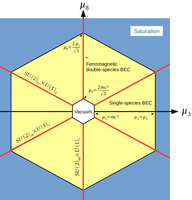
Figure 4: Schematic phase diagram of the $SU(3)$ quantum spin ladder in the $\mu_{3},\mu_{8}$-plane at zero temperature. For small values of the chemical potentials, the vacuum state exists in a hexagonal region. On the other hand, for large values of the chemical potentials, outside of a large hexagon, the system saturates. In the region between the two hexagons, there exist different types of single-species Bose-Einstein “condensates” (BEC). Generically, the chemical potentials break the global $SU(3)$ symmetry explicitly down to $U(1)_{3}\times U(1)_{8}$. However, along the $\mu_{8}$-axis the symmetry is enhanced to $SU(2)_{ud}\times U(1)_{s}$. Similarly, along the two lines at a 60 degree angle with respect to the $\mu_{8}$-axis, the symmetry is enhanced to $SU(2)_{ds}\times U(1)_{u}$ or $SU(2)_{su}\times U(1)_{d}$. Along the lines of enhanced symmetry, there exist different ferromagnetic double-species Bose-Einstein “condensates”.

As we will conclude from Monte Carlo simulations, once the chemical potentials overcome the massgap, depending on the segment of the phase diagram, the bosons with quantum number combinations $u\overline{d}$, $u\overline{s}$, $d\overline{s}$, $d\overline{u}$, $s\overline{u}$, or $s\overline{d}$ are produced in a second order phase transition. For example, once $\mu_{3}>mc^{2}$ (while $\mu_{8}=0$) the particle density of the $u\overline{d}$ bosons increases continuously from zero. This is when the “condensed matter physics” of the ${\mathbb{C}P}(2)$ model sets in. It is then natural to ask what phase of matter the bosons are forming. If different bosons would attract each other, the system should phase separate. This is not what happens in this case. Instead, the bosons repel each other and form a gas. We will present numerical evidence that (at least at zero temperature) the ultracold bosonic gas “condenses”. More precisely, the $U(1)_{3}$ symmetry undergoes the Kosterlitz-Thouless phenomenon. In view of the Mermin-Wagner theorem, this is as close as a $(1+1)$-d system can come to Bose-Einstein condensation.

In other segments of the phase diagram, bosons with other quantum number combinations “condense”, and corresponding linear combinations of $U(1)_{3}$ and $U(1)_{8}$ undergo the Kosterlitz-Thouless phenomenon. These Bose-Einstein “condensates” consist of a single species of bosons with one of the six quantum number combinations listed above. While for $\mu_{3}>0$ and $|\mu_{8}|<\frac{1}{\sqrt{3}}\mu_{3}$ the bosons of type $u\overline{d}$ “condense”, such that the $U(1)_{3}=U(1)_{ud}$ (but not the $U(1)_{8}=U(1)_{s}$) symmetry is affected by the Kosterlitz-Thouless phenomenon, for $\mu_{3}>0$ and $\mu_{8}>\frac{1}{\sqrt{3}}\mu_{3}$, the bosons of type $u\overline{s}$ “condense”, i.e. the $U(1)_{us}$ (but not the $U(1)_{d}$) symmetry is affected by the Kosterlitz-Thouless phenomenon. Note that $U(1)_{su}$ and $U(1)_{d}$ are generated by

$$\frac{1}{2}(T^{3}+\sqrt{3}T^{8})=\frac{1}{2}\mbox{diag}(1,0,-1),\quad\frac{1}{2}(\sqrt{3}T^{3}-T^{8})=\frac{1}{2\sqrt{3}}\mbox{diag}(1,-2,1),$$ (3.1)

respectively. Analogously, $U(1)_{ds}$ and $U(1)_{u}$ are generated by

$$-\frac{1}{2}(T^{3}-\sqrt{3}T^{8})=\frac{1}{2}\mbox{diag}(0,1,-1),\quad-\frac{1}{2}(\sqrt{3}T^{3}+T^{8})=\frac{1}{2\sqrt{3}}\mbox{diag}(-2,1,1).$$ (3.2)

Indeed, for $\mu_{3}>0$ and $\mu_{8}<-\frac{1}{\sqrt{3}}\mu_{3}$, the bosons of type $s\overline{d}$ “condense”, and now the $U(1)_{ds}$ (but not the $U(1)_{u}$) symmetry is affected by the Kosterlitz-Thouless phenomenon. The situation is analogous for $\mu_{3}<0$.

A special situation arises when the $U(1)_{3}\times U(1)_{8}$ symmetry is enhanced to a non-Abelian symmetry. For example, when $\mu_{3}=0$ the $U(1)_{3}$ symmetry is enhanced to $SU(2)_{123}=SU(2)_{ud}$. In that case, two species of bosons — namely those of the types $u\overline{s}$ and $d\overline{s}$ — “condense”. As a consequence, now the $U(1)_{8}=U(1)_{s}$ symmetry is affected by the Kosterlitz-Thouless phenomenon. How does the corresponding double-species Bose-Einstein “condensate” realize the enhanced $SU(2)_{ud}$ symmetry? Interestingly, our Monte Carlo simulations demonstrate that the system is a ferromagnet with a conserved order parameter — the $SU(2)_{ud}$ vector $(T^{1},T^{2},T^{3})$. It should be stressed that the Mermin-Wagner theorem does not prevent ferromagnetism in $(1+1)$ dimensions.

At very large values of the chemical potentials, the system ultimately saturates. In particular, for $\mu_{3}>\mu_{s}$ and $|\mu_{8}|<\frac{1}{\sqrt{3}}\mu_{3}$ at zero temperature the spins on sublattice $A$ are in the state $u$ while the spins on sublattice $B$ are in the state $\overline{d}$. It is straightforward to determine the exact value of $\mu_{s}\propto J$ associated with saturation. We will present this calculation elsewhere. Similarly, for $\frac{1}{2}\mu_{3}+\frac{\sqrt{3}}{2}\mu_{8}>\mu_{s}$, $\mu_{3}>0$, and $\mu_{8}>\frac{1}{\sqrt{3}}\mu_{3}$ the spins on sublattice $A$ are still in the state $u$ while the spins on sublattice $B$ are now in the state $\overline{s}$. As a consequence, for large values of the chemical potentials there is a region (bounded by a large hexagon) in which the system saturates in one of the six states $u\overline{d}$, $u\overline{s}$, $d\overline{s}$, $d\overline{u}$, $s\overline{u}$, and $s\overline{d}$.

It is interesting to ask whether there are other additional phases at intermediate values of the chemical potentials, before one reaches saturation. We will address this question in the future. In this paper, we concentrate on moderate values of the chemical potentials and we establish the existence of two non-trivial phases — the single-species Bose-Einstein “condensate” for $\mu_{3}>mc^{2}$, $\mu_{8}=0$, and the double-species ferromagnet for $\mu_{3}=0$, $\mu_{8}>\frac{2}{\sqrt{3}}mc^{2}$.

The previous discussion of the phase diagram referred to strictly zero temperature. Then the $(1+1)$-d quantum system experiences the Kosterlitz-Thouless phenomenon, i.e. bosons “condense” and the correlation length (of the infinite system with both $L\rightarrow\infty$ and inverse temperature $\beta\rightarrow\infty$) diverges. Even at an infinitesimally small non-zero temperature, the correlation length becomes finite and the previously discussed phase transitions (as a function of $\mu_{3}$ and $\mu_{8}$ at zero temperature) are washed out to smooth cross-overs.

3.2 Spinwave Velocity

First of all, it is useful to determine the low-energy parameters of the $(2+1)$-d ${\mathbb{C}P}(2)$ effective field theory before dimensional reduction. These are the spin stiffness $\rho_{s}$ and the spinwave velocity $c$. Here we determine the value of $c$ using the method described in [45], which results in $c=1.7763(2)Ja$ (where $J$ is the exchange coupling and $a$ is the lattice spacing). In the continuum limit (which is approached by gradually increasing $L^{\prime}$) the $(1+1)$-d ${\mathbb{C}P}(2)$ model results as a relativistic quantum field theory via dimensional reduction. As a consequence of the emerging symmetry between space and Euclidean time, the correlation lengths $\xi$ and $\xi_{t}$ in space and time should be related by $\xi=c\xi_{t}$. By measuring the exponential decay of the 2-point function $\langle T_{x}^{a}T_{y}^{a}\rangle$ at vanishing chemical potentials ($\mu_{3}=\mu_{8}=0$), we have explicitly verified this relation.

3.3 Single-Particle States

The mass gap separates the vacuum from an $SU(3)$ octet of massive particles with a rest energy $mc^{2}=1/\xi_{t}$ (or equivalently a rest mass $m=1/(c\xi)$). For $L^{\prime}/a=10,12,14$ and $L/a=250$ we obtain the rest energy values $mc^{2}=0.1006(1)J$, $0.05873(1)J$, and $0.0344(1)J$, respectively, which correspond to spatial correlation lengths (or equivalently Compton wave lengths) $\xi=17.66(2)a$, $30.25(1)a$, and $51.6(2)a$. This confirms the exponential increase of $\xi$ (cf. eq.(2.14)) which is a signature of asymptotic freedom. Note that $\xi\ll L$, such that finite-size effects can be neglected.

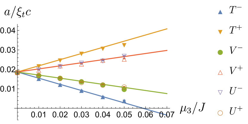
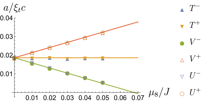
Figure 5: Inverse correlation lengths as a function of $\mu_{3}$, putting $\mu_{8}=0$ (top), and as a function of $\mu_{8}$, putting $\mu_{3}=0$ (bottom). The Monte Carlo data confirm that the eigenvalues of $H-\mu_{a}T^{a}$ are linear functions of the chemical potentials. The slopes of the straight lines (which are analytic predictions and not fits) are determined by the charges $(T^{3},T^{8})$ of the corresponding single-particle states.

In order to verify that the massive single-particle states indeed form an $SU(3)$ octet, we have analyzed the exponential decay of the Euclidean-time correlation functions of the various states both as a function of $\mu_{3}$ and $\mu_{8}$. The eigenvalues of $H-\mu_{a}T^{a}$ for the various single-particle states (at zero spatial momentum) are given by $mc^{2}-\mu_{3}T^{3}-\mu_{8}T^{8}$, and are thus linear functions of the chemical potentials. Fig.5 shows the corresponding inverse correlation lengths extracted from correlation functions associated with the $SU(3)$ shift operators $T^{\pm}$, $U^{\pm}$, and $V^{\pm}$ (cf. eq.(2.2)) as functions of $\mu_{3}$ (putting $\mu_{8}=0$) and as functions of $\mu_{8}$ (putting $\mu_{3}=0$). Acting on the vacuum, the various shift operators generate six single-particle states that are members of an $SU(3)$ octet with the quantum number combinations $(T^{3},T^{8})=(\pm 1,0)$, $(\pm\frac{1}{2},\pm\frac{\sqrt{3}}{2})$. Indeed, these quantum numbers are verified by the observed linear $\mu_{3}$- and $\mu_{8}$-dependencies of the corresponding inverse correlation lengths.

3.4 Leaving the Vacuum: the Onset of Particle Production

In this subsection we investigate the critical values of the chemical potentials that separate the vacuum sector of the phase diagram from the particle sectors in which the “condensed matter physics” of the ${\mathbb{C}P}(2)$ model takes place. We will address the nature of the phase formed by these particles (the Bose-Einstein “condensates” mentioned above) in the next subsection.

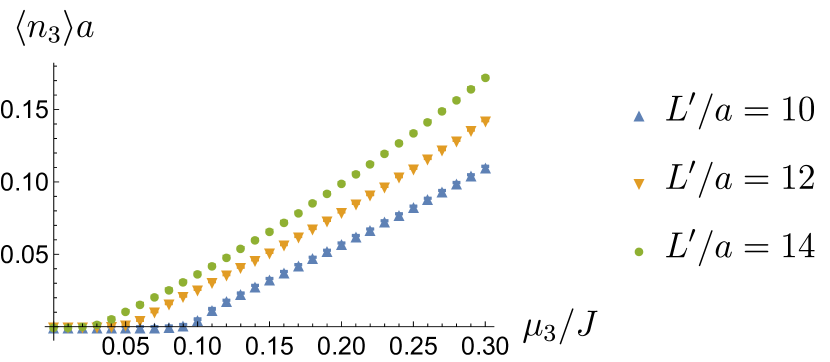
Figure 6: Particle density $\langle n_{3}\rangle$ as a function of $\mu_{3}$ (putting $\mu_{8}=0$) for three different values of $L^{\prime}$ over a wide range of $\mu_{3}$ (top) and zooming into a narrower range around the onsets (bottom), keeping $\beta c=L=250a$ fixed. The critical values $\mu_{3}=mc^{2}$ for the onset of particle production at zero temperature are indicated by the three dashed lines, corresponding to $L^{\prime}/a=10,12,14$.

Let us consider the effect of a chemical potential $\mu_{3}>0$, $\mu_{8}=0$ on the expectation value

$$\langle n_{3}\rangle=\frac{1}{L}\langle T^{3}\rangle,$$ (3.3)

which plays the role of the density of the particles of type $u\overline{d}$ (cf. Fig.6). Indeed, as indicated by the dashed lines, we see that the onset of particle production occurs near $\mu_{3}=mc^{2}$. At zero temperature, no particles should be produced below this critical value. For finite temperature, on the other hand, particles can also be produced by thermal fluctuations, thus washing out the onset behavior. Here the inverse temperature was fixed to $\beta J=140.75$ and again $L/a=250$. This corresponds to a square-shaped Euclidean space-time volume with $L=\beta c$.

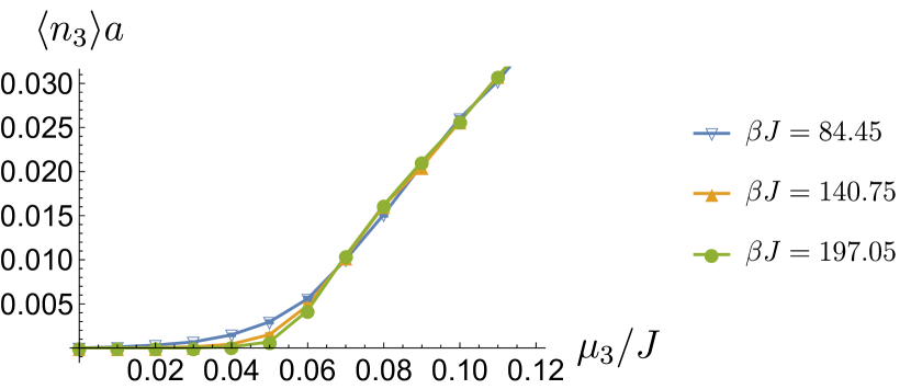
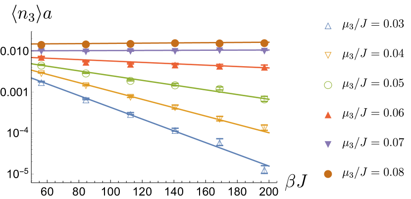
Figure 7: Particle density $\langle n_{3}\rangle$ as a function of $\mu_{3}$ (putting $\mu_{8}=0$) for three different inverse temperatures $\beta$, with lines to guide the eye (top), and as a function of $\beta$ for six different values of $\mu_{3}$ with exponential fits (bottom). Below the critical chemical potential $\mu_{3}=mc^{2}$, the particle density vanishes in the zero-temperature limit.

For the rest of the paper we set $L^{\prime}/a=12$, which puts us comfortably close to the continuum limit. In order to investigate finite-temperature and finite-volume effects in the onset region, in Fig.7 we compare $\langle n_{3}\rangle$ for three values of the inverse temperature $\beta J=56.3$, $140.75$, and $197.05$. Indeed, as long as $\mu_{3}<mc^{2}$, the particle density goes to zero with decreasing temperature, while for $\mu_{3}>mc^{2}$ it approaches a non-zero value. This is confirmed by logarithmically plotting the same data as a function of $\beta$ now keeping $\mu_{3}$ fixed (cf. Fig.7). In particular, we now see that the particle density $\langle n_{3}\rangle$ decreases exponentially with $\beta$ for $\mu_{3}<mc^{2}$.

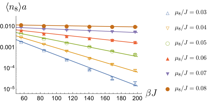
Figure 8: Particle density $\langle n_{8}\rangle$ as a function of $\mu_{8}$ (putting $\mu_{3}=0$) for three different inverse temperatures $\beta$, with lines to guide the eye (top), and as a function of $\beta$ for six different values of $\mu_{8}$ with exponential fits (bottom). Below the critical chemical potential $\mu_{8}=2mc^{2}/\sqrt{3}$, the particle density vanishes in the zero-temperature limit.

Let us now consider the situation with $\mu_{3}=0$ and $\mu_{8}>0$. Then the chemical potentials break the $SU(3)$ symmetry explicitly down to $SU(2)_{ud}\times U(1)_{s}$. In particular, now the particles of type $u\overline{s}$ and $d\overline{s}$ are both equally favored by the chemical potential $\mu_{8}$. The onset of the density

$$\langle n_{8}\rangle=\frac{1}{L}\langle T^{8}\rangle,$$ (3.4)

again for $\beta J=56.3$, $140.75$, and $197.05$, is illustrated in Fig.8. Note that the critical value for particle production is now given by $\mu_{8}=\frac{2}{\sqrt{3}}mc^{2}$, because the particles of type $u\overline{s}$ and $d\overline{s}$ have $T^{8}=\frac{\sqrt{3}}{2}$. As before, the data are replotted logarithmically as a function of $\beta$, which again shows an exponential suppression of the particle density $\langle n_{8}\rangle$ with temperature below the onset.

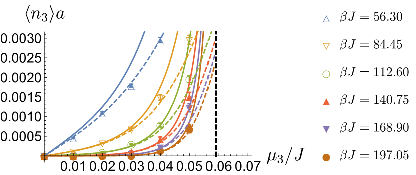
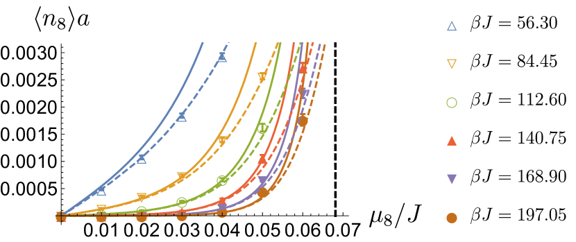
Figure 9: Particle density $\langle n_{3}\rangle$ as a function of $\mu_{3}$, putting $\mu_{8}=0$ (top), and $\langle n_{8}\rangle$ as a function of $\mu_{8}$, putting $\mu_{3}=0$ (bottom), for six different inverse temperatures $\beta$. Monte Carlo data are compared with a model of free bosons (solid lines) and a model of free fermions (dashed lines). The Monte Carlo data lie between the predictions of the bosonic and the fermionic model, indicating that the bosons of the ${\mathbb{C}P}(2)$ model are not free but repel each other.

In Fig.9 we compare the Monte Carlo data for $\langle n_{3}\rangle$ and $\langle n_{8}\rangle$ (at $\beta J=197.05$ and $L/a=300$) with analytic predictions of a free boson and a free fermion model. Although the massive particles in the $(1+1)$-d ${\mathbb{C}P}(2)$ model are bosons, they are not free but are expected to repel each other. In $(1+1)$-d, bosons with an infinite short-range repulsion are equivalent to free fermions. Indeed, the Monte Carlo data lie between the predictions of the free boson and the free fermion model, thus indicating that the ${\mathbb{C}P}(2)$ bosons have a finite repulsive interaction. Below the critical values of the chemical potentials, the particle density is very low. Consequently, both the bosonic and the fermionic model agree with each other. The fact that the Monte Carlo data of the ${\mathbb{C}P}(2)$ model are correctly represented in this regime (without fitting any parameters), confirms that the bosons of the ${\mathbb{C}P}(2)$ model indeed have the mass $m$.

The free boson model assumes that we have particles and anti-particles of mass $m$ with a relativistic dispersion relation $E(p)=\sqrt{(mc^{2})^{2}+(pc)^{2}}$ in a finite spatial interval of size $L$ with periodic boundary conditions. Hence, the momenta $p$ are quantized in integer multiples of $2\pi/L$. The particle densities are given by

$$\langle n_{3}\rangle=\frac{\partial\log Z(\beta,\mu_{3},\mu_{8})}{\partial(\beta\mu_{3})},\quad\langle n_{8}\rangle=\frac{\partial\log Z(\beta,\mu_{3},\mu_{8})}{\partial(\beta\mu_{8})}.$$ (3.5)

The grand canonical partition function factorizes in momentum and $T^{3}$ and $T^{8}$ quantum number sectors

$$Z(\beta,\mu_{3},\mu_{8})=\prod_{p,T^{3},T^{8}}Z_{p,T^{3},T^{8}}(\beta,\mu_{3},\mu_{8}),$$ (3.6)

with

$$Z_{p,T^{3},T^{8}}(\beta,\mu_{3},\mu_{8})=\sum_{n}\exp(-\beta(E(p)-\mu_{3}T^{3}-\mu_{8}T^{8})n).$$ (3.7)

For free bosons, the occupation numbers of each mode take values $n\in\{0,1,2,\dots,\infty\}$. In order to mimic boson repulsion, we also introduce a “fermionic” model, simply by restricting the occupation numbers to $n\in\{0,1\}$. One then obtains

$$\langle n_{3}\rangle = \frac{1}{L}\sum_{p,T^{3},T^{8}}\frac{T^{3}}{\exp(\beta(E(p)-\mu_{3}T^{3}-\mu_{8}T^{8}))\pm 1},$$

$$\langle n_{8}\rangle = \frac{1}{L}\sum_{p,T^{3},T^{8}}\frac{T^{8}}{\exp(\beta(E(p)-\mu_{3}T^{3}-\mu_{8}T^{8}))\pm 1}\ .$$ (3.8)

Here $\pm$ corresponds to fermions and bosons, respectively. Note that free bosons give rise to an infinite density once the chemical potentials reach their critical values. The sum extends over all momenta $p=2\pi l/L$ (with $l\in{\mathbb{Z}}$) and over the 8 particle and anti-particle states in the $SU(3)$ octet. The 2 states with $T^{3}=T^{8}=0$ do not contribute, because the corresponding particles are neutral.

It should be noted that the particles of the “fermionic” model are not truly relativistic two-component Dirac fermions, but rather one-component objects with fermionic statistics. This violates the spin-statistics theorem and is thus inconsistent with relativistic invariance. In any case, neither the results of the bosonic nor of the “fermionic” model are expected to describe the behavior of the ${\mathbb{C}P}(2)$ model completely correctly. They just indicate that the bosons of the ${\mathbb{C}P}(2)$ model repel each other. It would also be interesting to compare the Monte Carlo data with the non-relativistic Lieb-Liniger model [46]. This will be addressed elsewhere.

3.5 Single-Species Bose-Einstein “Condensation”

In this subsection, we put $\mu_{8}=0$ and study the physics as a function of $\mu_{3}$. We have investigated systems of two different sizes $L=300a$ and $600a$ (with fixed $L^{\prime}=12a$) at two different inverse temperatures $\beta J=197.05$ and $281.5$.

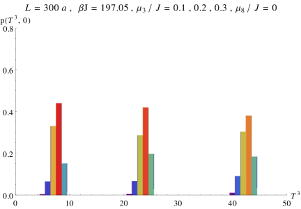
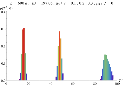
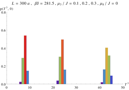
Figure 10: Probability distributions $p(T^{3},T^{8}=0)$ for three different values of the chemical potential $\mu_{3}=0.1,0.2,0.3$ and $\mu_{8}=0$. Lattice size and inverse temperature are fixed to $L=300a$, $\beta J=197.05$ (top), $L=600a$, $\beta J=197.05$ (middle), and $L=300a$, $\beta J=281.5$ (bottom).

The probability distributions of the different charge sectors $(T^{3},T^{8})$ are illustrated in Fig.10 (top) for $L=300a$ and $\beta J=197.05$ for $\mu_{3}/J=0.1,0.2,0.3$, and $\mu_{8}=0$. For $\mu_{3}=0.1J>mc^{2}$, we see the onset of particle production with $\langle T^{3}\rangle>0$. As expected for $\mu_{8}=0$, almost all states have $T^{8}=0$, which implies that the produced bosons carry the quantum number combination $u\overline{d}$. For $\mu_{3}=0.1J$, there are typically 8 bosons in the $L=300a$ box. Since the Compton wave length of the bosons is $\xi=1/(mc)=30.25a$, they are not very dilute at this value of $\mu_{3}$. When the chemical potential is increased further, the probability distribution is shifted to larger values of $T^{3}$. For $\mu=0.2J$ the most probable particle number is 24, and for $\mu_{3}=0.3J$ it is 43, which correspond to rather dense systems of bosons. Fig.10 (middle) shows the same situation for the larger spatial volume $L=600a$. Now, for a given value of $\mu_{3}$, about twice as many particles are being produced, but their density $\langle T^{3}\rangle/L$ remains more or less the same, indicating that finite-size effects are moderate. Fig.10 (bottom) shows results for the $L=300a$ box at the lower temperature corresponding to $\beta J=281.5$. As expected, thermal fluctuations in the charge (or equivalently particle number) distribution are then further suppressed. From these results we conclude that, as $\mu_{3}$ increases from $mc^{2}$ to $0.3J$, the system contains an increasing density of bosons of type $u\overline{d}$.

It is natural to ask what state of “${\mathbb{C}P}(2)$ condensed matter” these bosons are forming. As we will now demonstrate, not surprisingly, in the zero-temperature limit (given the limitations of the Mermin-Wagner theorem), they form a Bose-Einstein “condensate”. To study this, we have investigated the spatial winding numbers, $W_{3},W_{8}\in{\mathbb{Z}}$, for which

$$\langle W_{3}^{2}\rangle = \frac{\partial^{2}\log Z(\beta,L,L^{\prime},\mu_{3},\mu_{8},\theta_{3},\theta_{8})}{\partial\theta_{3}^{2}}\bigg{|}_{\theta_{3}=\theta_{8}=0},$$

$$\langle W_{8}^{2}\rangle = \frac{\partial^{2}\log Z(\beta,L,L^{\prime},\mu_{3},\mu_{8},\theta_{3},\theta_{8})}{\partial\theta_{8}^{2}}\bigg{|}_{\theta_{3}=\theta_{8}=0}.$$ (3.9)

Here $Z(\beta,L,L^{\prime},\mu_{3},\mu_{8},\theta_{3},\theta_{8})$ is the partition function of a system with twisted periodic boundary conditions in the spatial direction of size $L$. The twist is characterized by the matrix $\exp(i\theta_{3}T^{3}+i\theta_{8}T^{8})\in U(1)_{3}\times U(1)_{8}\subset SU(3)$. In the limit $L,\beta\rightarrow\infty$ we then obtain the helicity moduli

$$\Upsilon_{3}=\frac{L}{\beta}\langle W_{3}^{2}\rangle,\quad\Upsilon_{8}=\frac{L}{\beta}\langle W_{8}^{2}\rangle.$$ (3.10)

A non-vanishing helicity modulus signals strong sensitivity to the twisted boundary condition and hence the existence of an infinite correlation length associated with the Kosterlitz-Thouless phenomenon. The precise determination of the helicity moduli $\Upsilon_{3}$ and $\Upsilon_{8}$ requires a careful finite-size analysis, which will be addressed elsewhere.

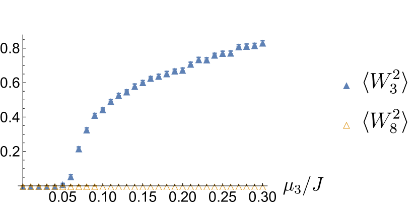
Figure 11: Expectation values $\langle W_{3}^{2}\rangle$ and $\langle W_{8}^{2}\rangle$ of the spatial winding numbers $W_{3}$ and $W_{8}$ as a function of $\mu_{3}$ for $\mu_{8}=0$. Lattice size and inverse temperature are fixed to $L=\beta c=250a$.

Fig.11 illustrates the $\mu_{3}$-dependence of $\langle W_{3}^{2}\rangle$ and $\langle W_{8}^{2}\rangle$ for $\mu_{8}=0$ with $L=\beta c=250a$ (with $\beta J=140.75$). Since the system contains bosons of type $u\overline{d}$ (which have $T^{8}=0$), one finds $\langle W_{8}^{2}\rangle=0$. Since these bosons (which appear in the system for $\mu_{3}>mc^{2}$) carry the charge $T^{3}=1$, we obtain $\langle W_{3}^{2}\rangle\neq 0$ when $\mu_{3}$ exceeds its critical value. The smooth onset of $\langle W_{3}^{2}\rangle$ confirms the second order nature of the phase transition. In view of the Mermin-Wagner theorem, we conclude that, for $\mu_{3}>mc^{2}$, the bosons of type $u\overline{d}$ undergo the Kosterlitz-Thouless phenomenon. The “condensation” affects the $U(1)_{3}$ symmetry, while the $U(1)_{8}$ symmetry remains unaffected.

It should be noted that the onset of “condensation” is not a Kosterlitz-Thouless phase transition. While the latter is driven by thermal fluctuations, below the onset of particle production, the system just exists in the vacuum state and simply looses its material basis for “${\mathbb{C}P}(2)$ condensed matter physics”.

3.6 Double-Species Ferromagnetic Bose-Einstein “Condensation”

Let us now consider the physics along the $\mu_{8}$-axis of the phase diagram, i.e. we now put $\mu_{3}=0$. The system then has an enhanced $SU(2)_{ud}\times U(1)_{s}$ symmetry. As we have seen before, when $\mu_{8}>\frac{2}{\sqrt{3}}mc^{2}$, bosons of the two types $u\overline{s}$ and $d\overline{s}$ are produced. Again, the question arises what phase of “${\mathbb{C}P}(2)$ condensed matter” these bosons form. Not surprisingly, as we will now show, they form a double-species Bose-Einstein “condensate”, which is now associated with the $U(1)_{8}$ symmetry. Interestingly, the $SU(2)_{ud}$ symmetry is realized as in a ferromagnet. Hence, we address this phase as a double-species ferromagnetic Bose-Einstein “condensate”. It should be noted that in a ferromagnet “spontaneous symmetry breaking” is qualitatively different than in an antiferromagnet. This is because the order parameter of the ferromagnet — namely the uniform magnetization or total spin — is a conserved quantity, while the staggered magnetization of an antiferromagnet is not conserved. In particular, this leads to a quadratic dispersion relation of ferromagnetic spinwaves. This is indeed what happens for the ferromagnetic Bose-Einstein “condensate”.

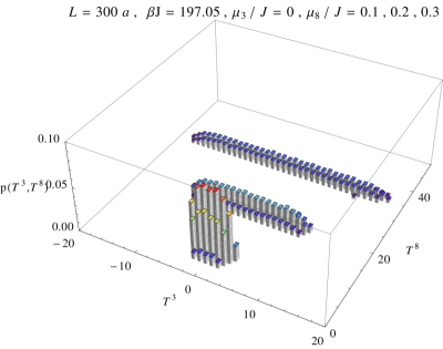
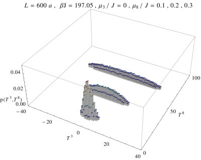
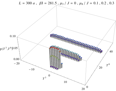
Figure 12: Probability distributions $p(T^{3},T^{8})$ for three different values of the chemical potential $\mu_{8}=0.1,0.2,0.3$ and $\mu_{3}=0$. Lattice size and inverse temperature are fixed to $L=300a$, $\beta J=197.05$ (top), $L=600a$, $\beta J=197.05$ (middle), and $L=300a$, $\beta J=281.5$ (bottom).

Fig.12 (top) shows the probability distributions of the various charge sectors $(T^{3},T^{8})$ for $\mu_{8}/J=0.1,0.2,0.3$ with $L=\beta c=300a$ and $\beta J=197.05$. Below the threshold for particle production (at $\mu_{8}=0.03J<\frac{2}{\sqrt{3}}mc^{2}$), up to small thermal fluctuations, the system stays in the vacuum sector with $T^{3}=T^{8}=0$. For $\mu_{8}>\frac{2}{\sqrt{3}}mc^{2}$, on the other hand, states with $\langle T^{8}\rangle>0$ are generated. The most probable values of $\frac{2}{\sqrt{3}}T^{8}$ for $\mu_{8}/J=0.1,0.2,0.3$ are $6,19,35$, respectively. While the thermal fluctuations of $T^{8}$ are rather small, $T^{3}$ varies over the whole range $|T^{3}|\leq T^{8}/\sqrt{3}$ because bosons of both types $u\overline{s}$ and $d\overline{s}$ are equally favored by the chemical potential $\mu_{8}$. Fig.12 (middle) shows data for the larger spatial volume $L=600a$, keeping the temperature unchanged. As before, for a given value of $\mu_{8}$, about twice as many particles are being produced, but their density $\langle T^{8}\rangle/L$ remains essentially unchanged. This again indicates that finite-size effects are under control. Fig.12 (bottom) shows results for the $L=300a$ box at the lower temperature corresponding to $\beta J=281.5$. Again, thermal fluctuations in the charge distribution are then further suppressed. We conclude that, as $\mu_{8}$ increases from $\frac{2}{\sqrt{3}}mc^{2}$ to $0.3J$, the system contains an increasing density of bosons of type $u\overline{s}$ or $d\overline{s}$.

It is interesting to note that the probability distribution is rather flat as a function of $T^{3}$, at least at low temperatures and as long as $|T^{3}|\leq T^{8}/\sqrt{3}$. This indicates that, in the zero temperature limit, the system has a degenerate ground state with a large value $T=T^{8}/\sqrt{3}$ for the length of the $SU(2)_{ud}$ vector $(T^{1},T^{2},T^{3})$. The total number of bosons of type $u\overline{s}$ or $d\overline{s}$ (which each have $T^{8}=\frac{\sqrt{3}}{2}$) is given by $N=\frac{2}{\sqrt{3}}T^{8}$. The bosons $u\overline{s}$ and $d\overline{s}$ form a doublet with $T=\frac{1}{2}$, and $T^{3}=\pm\frac{1}{2}$. Hence $N$ of these bosons can form a state with maximal total charge $T=\frac{N}{2}=T^{8}/\sqrt{3}$, which is indeed what the Monte Carlo data indicate. Such a state is totally symmetric under the permutation of the flavor indices of the $N$ bosons. Hence, their orbital wave function must also be totally symmetric. This is exactly what one expects for a Bose-Einstein condensate. Since the vector $(T^{1},T^{2},T^{3})$ (just like the total spin of a ferromagnet) serves as a conserved order parameter for this state, we are confronted with a two-component ferromagnetic Bose-Einstein “condensate”. In this case, the Abelian $U(1)_{8}=U(1)_{s}$ subgroup of the $SU(2)_{ud}\times U(1)_{s}$ symmetry is affected by the Kosterlitz-Thouless phenomenon, while the non-Abelian $SU(2)_{ud}$ symmetry is realized ferromagnetically.

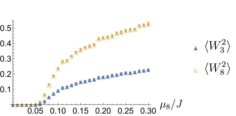
Figure 13: Expectation values $\langle W_{3}^{2}\rangle$ and $\langle W_{8}^{2}\rangle$ of the spatial winding numbers $W_{3}$ and $W_{8}$ as a function of $\mu_{8}$ for $\mu_{3}=0$. Lattice size and inverse temperature are fixed to $L=\beta c=250a$.

In order to confirm that the bosons indeed “condense”, we have again investigated the spatial winding numbers. Fig.13 shows $\langle W_{3}^{2}\rangle$ and $\langle W_{8}^{2}\rangle$ as a function of $\mu_{8}$ for $\mu_{3}=0$. Since the bosons of type $u\overline{s}$ and $d\overline{s}$ bosons have $T^{8}=\frac{\sqrt{3}}{2}$, in this case not only $\langle W_{3}^{2}\rangle\neq 0$ but also $\langle W_{8}^{2}\rangle\neq 0$ beyond the threshold $\mu_{8}=2mc^{2}/\sqrt{3}$. The smooth onset again indicates the second order nature of the phase transition.

4 Conclusions

We have investigated the $(1+1)$-d ${\mathbb{C}P}(2)$ model in an unconventional regularization, in which the model results via dimensional reduction from a $(2+1)$-d antiferromagnetic $SU(3)$ quantum spin ladder, which is particularly well suited for quantum simulation experiments using ultracold alkaline-earth atoms in an optical superlattice. The continuum limit of the dimensionally reduced model is approached by gradually increasing the transverse extent $L^{\prime}=na$ of the ladder. Here we have considered even values of $n$, which corresponds to the vacuum angle $\theta=0$.

Quantum simulation experiments have been proposed to study ${\mathbb{C}P}(N-1)$ models in real-time as well as at non-zero chemical potential [33, 32] . This will serve as a test case for the more long-term goal of quantum simulating QCD in real time or at large baryon chemical potential. Due to very severe sign problems, these dynamics are impossible to address with Monte Carlo simulations on classical computers. Fortunately, the “condensed matter physics” of ${\mathbb{C}P}(N-1)$ models can be investigated without encountering a sign problem, using an efficient worm algorithm applied to the underlying $SU(N)$ quantum spin system. This can be used to validate future implementations of ${\mathbb{C}P}(N-1)$ quantum simulators. This will help to pave the way towards quantum simulations of $U(N)$ and $SU(N)$ non-Abelian gauge theories, ultimately including QCD, which can again be realized with ultracold alkaline-earth atoms [27] .

Using a worm algorithm for an $SU(3)$ quantum spin ladder, we have investigated the phase diagram of the $(1+1)$-d ${\mathbb{C}P}(2)$ model as a function of the two chemical potentials $\mu_{3}$ and $\mu_{8}$. The vacuum is realized at zero temperature when the chemical potentials are below their critical values, which are determined by the mass gap of the $SU(3)$ octet of lightest particles. We have concentrated on investigating the phase diagram along the $\mu_{3}$- and $\mu_{8}$-axes. For $\mu_{3}>mc^{2},\mu_{8}=0$ the bosons of type $u\overline{d}$ form a Bose-Einstein “condensate”, i.e. the $U(1)_{3}$ subgroup of the $U(1)_{3}\times U(1)_{8}$ symmetry is affected by the Kosterlitz-Thouless phenomenon. Along the $\mu_{8}$-axis (i.e. for $\mu_{3}=0$), on the other hand, an enhanced symmetry $SU(2)_{ud}\times U(1)_{s}\subset SU(3)$ exists. Then for $\mu_{8}>\frac{2}{\sqrt{3}}mc^{2}$, bosons of both types $u\overline{s}$ and $d\overline{s}$ are equally favored by the chemical potential. Now the $U(1)_{8}$ symmetry is affected by the Kosterlitz-Thouless phenomenon, which gives rise to a double-species Bose-Einstein “condensate”. Interestingly, the $SU(2)_{ud}$ symmetry is realized as in a ferromagnet. Indeed, the conserved spin vector $(T^{1},T^{2},T^{3})$ picks up a non-zero expectation value, which means that the system forms a ferromagnet.

In the future, it would be interesting to further extend the investigation of the ${\mathbb{C}P}(2)$ phase diagram, away from the axes and to larger values of the chemical potentials. For very large values of $\mu_{3}$ and $\mu_{8}$ the $SU(3)$ quantum spins of the underlying antiferromagnetic ladder system will completely align, forming a trivial saturated state. It will be interesting to investigate whether the single- and double-species Bose-Einstein “condensates” persist until saturation, or whether there are further phases of ${\mathbb{C}P}(2)$ “condensed matter” yet to be discovered. Furthermore, it will also be worth studying the phase diagram for vacuum angle $\theta=\pi$, which corresponds to an odd number $n$ of transversely coupled quantum spin chains. Then charge conjugation is spontaneously broken in the vacuum, and it is interesting to investigate how this affects the phase diagram.

Our study shows that ${\mathbb{C}P}(N-1)$ models, which share many features with QCD, have a rich “condensed matter” physics. In contrast to QCD, fortunately ${\mathbb{C}P}(N-1)$ models at non-zero chemical potential can be studied with efficient quantum Monte Carlo simulations on classical computers. This can be used to validate future quantum simulation experiments of ${\mathbb{C}P}(N-1)$ models which — just like quantum simulations of $SU(N)$ gauge theories — can be realized with ultracold alkaline-earth atoms in optical lattices. Quantum simulation experiments of ${\mathbb{C}P}(N-1)$ models thus form a natural first step towards the ultimate long-term goal of quantum simulating QCD.

Appendix A Monte Carlo Method

To study the $(2+1)$-d antiferromagnetic $SU(3)$ quantum spin ladder introduced in Section 2 we have implemented a worm algorithm in discrete Euclidean time. In [41] a meron-cluster algorithm was used to solve the sign problem at non-zero chemical potential in the ${\mathbb{C}P}(1)=O(3)$ model. Here the ${\mathbb{C}P}(2)$ model is simulated using a worm algorithm, which is capable of updating the system at non-zero chemical potential without encountering a sign problem [42]. This method is analogous to the $SU(2)$ case studied in [47]. For simplicity, we discuss the algorithm in discrete Euclidean time although it is straightforward to implement it directly in the Euclidean time continuum [48].

A.1 Path Integral Representation of the Grand Canonical Partition Function

In order to construct a discrete Euclidean time path integral for the quantum spin ladder, the Hamiltonian is split into four non-commuting pieces $H=H_{1}+H_{2}+H_{3}+H_{4}$,

$$H_{1} =J\sum_{x\in A}T^{a}_{x}\overline{T}^{a}_{x+\hat{1}}\,, H_{2} =J\sum_{x\in A}T^{a}_{x}\overline{T}^{a}_{x+\hat{2}}\,,$$

$$H_{3} =J\sum_{x\in A}T^{a}_{x}\overline{T}^{a}_{x-\hat{1}}\,, H_{4} =J\sum_{x\in A}T^{a}_{x}\overline{T}^{a}_{x-\hat{2}}\,.$$ (A.1)

It should be noted that bonds that extend beyond the open boundary must be omitted from the sums in $H_{2}$ and $H_{4}$. Using the Suzuki-Trotter formula, the partition function takes the form

$$Z =\operatorname{Tr}\exp\left(-\beta\left(H-\mu_{a}T^{a}\right)\right)=\lim_{\begin{subarray}{c}\epsilon\to 0\\ \epsilon M=\beta\end{subarray}}\operatorname{Tr}\left(\prod_{i=1}^{4}\exp\left(-\epsilon\left(H_{i}-\frac{\mu_{a}T^{a}}{4}\right)\right)\right)^{M}$$

$$=\sum_{[f]}\exp\left(-S[f]\right)\,.$$ (A.2)

Between all transfer matrix factors a complete set of eigenstates $\left|f_{x}\right>$ of $T_{x}^{3}$ and $T_{x}^{8}$ (with $f_{x}\in\{u,d,s\}$ on even sites $x\in A$) or $\left|\bar{f}_{y}\right>$ of $\overline{T}_{y}^{3}$ and $\overline{T}_{y}^{8}$ (with $\bar{f}_{y}\in\{\bar{u},\bar{d},\bar{s}\}$ on odd sites $y\in B$) is inserted. This yields a (2+1)-d system whose additional dimension is Euclidean time, which extends over $4M$ time-slices. Since each $H_{i}$ consists of commuting contributions $h_{xy}=JT^{a}_{x}\overline{T}^{a}_{y}$, the Boltzmann weight $\exp(-S[f])$ of a quantum spin configuration $[f]$ is a product over space-time plaquettes associated with a nearest-neighbor pair of spins as well as over individual sites at the open boundary

$$\exp(-S[f])= \prod_{x\in A,t=4p-3}W_{f_{x,t}\bar{f}_{x+\hat{1},t}}^{f^{\prime}_{x,t+1}\bar{f}^{\prime}_{x+\hat{1},t+1}}\prod_{x\in A,t=4p-2}W_{f_{x,t}\bar{f}_{x+\hat{2},t}}^{f^{\prime}_{x,t+1}\bar{f}^{\prime}_{x+\hat{2},t+1}}$$

$$\prod_{x\in A,t=4p-1}W_{f_{x,t}\bar{f}_{x-\hat{1},t}}^{f^{\prime}_{x,t+1}\bar{f}^{\prime}_{x-\hat{1},t+1}}\prod_{x\in A,t=4p}W_{f_{x,t}\bar{f}_{x-\hat{2},t}}^{f^{\prime}_{x,t+1}\bar{f}^{\prime}_{x-\hat{2},t+1}}$$

$$\prod_{x\in A,x_{2}\in\{1,L^{\prime}/a\},t=4p}W_{f_{x,t}}^{f^{\prime}_{x,t+1}}\prod_{y\in B,y_{2}\in\{1,L^{\prime}/a\},t=4p}W_{\bar{f}_{y,t}}^{\bar{f}^{\prime}_{y,t+1}}\,.$$ (A.3)

The last two products extend over points at the open boundaries in the 2-direction. It should again be noted that bonds extending beyond the open boundary must be omitted from the second and fourth product. The integer $p$ extends from 1 to $M$.

The plaquette weight takes the form

$$W_{f_{x,t}\bar{f}_{x,t}}^{f^{\prime}_{x,t+1}\bar{f}^{\prime}_{y,t+1}}=\left<f_{x,t}\bar{f}_{y,t}\vphantom{\exp\left(-\epsilon\left(h_{xy}-\frac{\mu_{a}T_{x}^{a}+\mu_{a}\overline{T}_{y}^{a}}{4}\right)\right)f_{x,t+1}^{\prime}\bar{f}_{y,t+1}^{\prime}}\right|\exp\left(-\epsilon\left(h_{xy}-\frac{\mu_{a}T_{x}^{a}+\mu_{a}\overline{T}_{y}^{a}}{4}\right)\right)\left|f_{x,t+1}^{\prime}\bar{f}_{y,t+1}^{\prime}\vphantom{f_{x,t}\bar{f}_{y,t}\exp\left(-\epsilon\left(h_{xy}-\frac{\mu_{a}T_{x}^{a}+\mu_{a}\overline{T}_{y}^{a}}{4}\right)\right)}\right>\,.$$ (A.4)

It is non-negative and has the following non-zero entries for $f\neq f^{\prime}$

$$W_{f\bar{f}}^{f\bar{f}} =\exp\left(\frac{\epsilon J}{6}\right)\frac{1}{3}\left(\exp\left(\frac{3\epsilon J}{2}\right)+2\right)=:W_{A}\,,$$

$$W_{f\bar{f}}^{f^{\prime}\bar{f}^{\prime}} =\exp\left(\frac{\epsilon J}{6}\right)\frac{1}{3}\left(\exp\left(\frac{3\epsilon J}{2}\right)-1\right)=:W_{B}\,,$$

$$W_{f\bar{f}^{\prime}}^{f\bar{f}^{\prime}} =\exp\left(\frac{\epsilon J}{6}\right)\exp\left(\frac{\epsilon}{4}\left(\mu_{3}t_{f}^{3}+\mu_{3}t_{\bar{f}^{\prime}}^{3}+\mu_{8}t_{f}^{8}+\mu_{8}t_{\bar{f}^{\prime}}^{8}\right)\right)=:W_{f\bar{f}^{\prime}}\,,$$ (A.5)

where $t^{3}_{f},t^{8}_{f},t^{3}_{\bar{f}},t^{8}_{\bar{f}}$ correspond to the charges of $f\in\{u,d,s\}$ and $\bar{f}\in\{\bar{u},\bar{d},\bar{s}\}$

$$t^{3}_{u} =-t^{3}_{\bar{u}}=\frac{1}{2}\,, t^{8}_{u}=-t^{8}_{\bar{u}} =\frac{1}{2\sqrt{3}}\,,$$

$$t^{3}_{d} =-t^{3}_{\bar{d}}=-\frac{1}{2}\,, t^{8}_{d}=-t^{8}_{\bar{d}} =\frac{1}{2\sqrt{3}}\,,$$

$$t^{3}_{s} =-t^{3}_{\bar{s}}=0\,, t^{8}_{s}=-t^{8}_{\bar{s}} =-\frac{1}{\sqrt{3}}\,.$$ (A.6)

The weights associated with time-like bonds for points at the open boundary take the form

$$W_{f_{x,t}}^{f_{x,t+1}^{\prime}}=\left<f_{x,t}\vphantom{\exp\left(\frac{\epsilon\mu_{a}T_{x}^{a}}{4}\right)f_{x,t+1}^{\prime}}\right|\exp\left(\frac{\epsilon\mu_{a}T_{x}^{a}}{4}\right)\left|f_{x,t+1}^{\prime}\vphantom{f_{x,t}\exp\left(\frac{\epsilon\mu_{a}T_{x}^{a}}{4}\right)}\right>\,,$$

$$W_{\bar{f}_{y,t}}^{\bar{f}_{y,t+1}^{\prime}}=\left<\bar{f}_{y,t}\vphantom{\exp\left(\frac{\epsilon\mu_{a}\overline{T}_{y}^{a}}{4}\right)\bar{f}_{y,t+1}^{\prime}}\right|\exp\left(\frac{\epsilon\mu_{a}\overline{T}_{y}^{a}}{4}\right)\left|\bar{f}_{y,t+1}^{\prime}\vphantom{\bar{f}_{y,t}\exp\left(\frac{\epsilon\mu_{a}\overline{T}_{y}^{a}}{4}\right)}\right>\,.$$ (A.7)

It has non-zero entries only for $f_{x,t}=f^{\prime}_{x,t+1}$, which are given by

$$W_{f}^{f} =\exp\left(\frac{\epsilon}{4}\left(\mu_{3}t^{3}_{f}+\mu_{8}t^{8}_{f}\right)\right)=:W_{f}\,,$$ (A.8)

$$W_{\bar{f}}^{\bar{f}} =\exp\left(\frac{\epsilon}{4}\left(\mu_{3}t^{3}_{\bar{f}}+\mu_{8}t^{8}_{\bar{f}}\right)\right)=:W_{\bar{f}}\,.$$ (A.9)

A.2 Worm Algorithm

After Trotter decomposition, the configurations of the $SU(3)$ quantum spin ladder can be sampled with a worm algorithm respecting detailed balance and ergodicity. This algorithm is analogous to the $SU(2)$ case discussed in [47]. In order to move from one allowed configuration to the next, the worm algorithm proceeds via configurations for which $SU(3)$ spin conservation is violated at two space-time points associated with the worm-head and the worm-tail. The worm-head is moved around by a local Metropolis algorithm, until it ultimately meets the tail and the worm closes. In that moment spin conservation is again restored and one obtains a new allowed configuration. By histograming the position of the worm-head relative to the worm-tail one obtains information about the two-point-functions of the shift operators $T^{\pm},U^{\pm},V^{\pm}$. In addition, by counting how often the worm-head wraps around the periodic spatial or temporal boundaries (before it meets the tail) one can determine the changes in the spatial and temporal winding numbers $W_{3},W_{8}$ and $T^{3},T^{8}$. The worm algorithm proceeds in the following steps:

1. Consider a valid initial configuration $[f^{(0)}]$ of $SU(3)$ quantum spin variables.

2. Select a space-time point $x_{0},t_{0}$ at random as the initial position of the worm-head and -tail, as well as an initial time-direction $D=D_{0}=\pm$. Identify the flavor $f=f_{x_{0},t_{0}}$ (or $\bar{f}=\bar{f}_{y_{0},t_{0}}$ for sites $y_{0}$ on sublattice $B$). Choose a flavor $f^{\prime}$ different from $f$ at random, and identify the charges carried by the worm as $\Delta^{3,8}=D_{0}(t_{f^{\prime}}^{3,8}-t_{f}^{3,8})$.

3. Identify the plaquette (or time-like bond for points at the open boundary) at the position $x,t$ of the worm-head in direction $D$. Choose an exit point $x^{\prime},t^{\prime}$ on this plaquette (or time-like bond) according to the probability denoted by $p_{\Delta^{3,8}}\left(x^{\prime},t^{\prime}|x,t;\{f\}\right)$ (cf. Table 3), where $\{f\}$ refers to the configuration of the plaquette (or time-like bond) before the move of the worm-head. Then move the worm-head to the new position $x^{\prime},t^{\prime}$. If $x^{\prime},t^{\prime}$ agrees with $x,t$ the worm-head bounces, i.e. it changes its direction. Increment the histogram of the two-point-function of the corresponding shift operators. Also record the contribution to the spatial and temporal winding number changes, according to the direction of the motion of the worm-head.

4. Determine the new worm direction $D^{\prime}$. If $t^{\prime}=t$, set $D^{\prime}=-D$, otherwise $D^{\prime}=D$.

5. Update the quantum spin at $x^{\prime},t^{\prime}$ by adding $D^{\prime}\Delta^{3}$ to $t^{3}_{f_{x^{\prime},t^{\prime}}}$ and $D^{\prime}\Delta^{8}$ to $t^{8}_{f_{x^{\prime},t^{\prime}}}$. As an example consider, a worm with charges $\Delta^{3}=1$ and $\Delta^{8}=0$. Moving forward in time, a flavor $d$ will be updated to $u$ and a flavor $\bar{u}$ to $\bar{d}$. Moving backward in time, a flavor $u$ will be updated to $d$ and a flavor $\bar{d}$ to $\bar{u}$.

6. Now replace $D$ by $D^{\prime}$. If $x^{\prime},t^{\prime}$ is different from $x_{0},t_{0}$, i.e. as long as the worm-head has not met the tail, proceed with step 3. If $x^{\prime},t^{\prime}$ agrees with $x_{0},t_{0}$, i.e. if the worm has closed, proceed with step 2 until the desired statistics is achieved.

The probabilities $p_{\Delta^{3,8}}\left(x^{\prime},t^{\prime}|x,t,\{f\}\right)$ are constrained by detailed balance and normalization conditions. Syljuåsen and Sandvik outlined a procedure to state these conditions in the form of several decoupled sets of linear equations for a general nearest-neighbor interaction [47]. Here we extend their $SU(2)$ algorithm to $SU(3)$. We separately consider each worm-type characterized by the charge that it carries. The resulting sets of equations for a worm that carries the charges $\Delta^{3}=-1$ and $\Delta^{8}=0$ are shown in Tables 1 and 2 alongside a visualization of the corresponding worm moves analogous to the ones in [47]. For worms carrying other charges, the corresponding systems can be obtained by flavor permutations. In addition to the systems of type $(I)$ (which are of the same form as the ones discussed in [47] for $SU(2)$), we have to consider situations where a worm encounters a plaquette containing the third flavor or an open boundary. These lead to the systems of equations of type $(II)$ to $(IV)$ (cf. Table 2). All systems are under-determined, but can be solved uniquely by imposing the non-negativity of all weights and minimizing the sum of all bounce weights $\sum_{i=1}^{9}(b_{i}+b_{i}^{\prime})$, which strongly affects the efficiency of the algorithm.

Type (I)
		$\begin{array}[]{rl}b_{1}+a+b&=W_{A}\\ \\ a+b_{2}+c&=W_{B}\\ \\ b+c+b_{3}&=W_{d\overline{u}}\end{array}$
		$\begin{array}[]{rl}b_{1}^{\prime}+a^{\prime}+b^{\prime}&=W_{A}\\ \\ a^{\prime}+b_{2}^{\prime}+c^{\prime}&=W_{B}\\ \\ b^{\prime}+c^{\prime}+b_{3}^{\prime}&=W_{u\overline{d}}\end{array}$

Table 1: Worm equations of type $(I)$. Space-time plaquette configurations ${}_{f_{x,t}\bar{f}_{x,t}}^{f^{\prime}_{x,t+1}\bar{f}^{\prime}_{y,t+1}}$ are shown together with the path taken by the worm-head. Its entrance and exit points are denoted by a dot and an arrow-head, respectively. The corresponding normalization conditions for the bounce weights $b_{i}$ and the weights $a,b,c$ for space-like, time-like, and diagonal moves are shown on the right.

Type (II)
	$\begin{array}[]{rl}b_{4}+d&=W_{u\bar{s}}\\ \\ d+b_{5}&=W_{d\bar{s}}\end{array}$		$\begin{array}[]{rl}b_{4}^{\prime}+d^{\prime}&=W_{s\bar{d}}\\ \\ d^{\prime}+b_{5}^{\prime}&=W_{s\bar{u}}\end{array}$
Type (III)
	$\begin{array}[]{rl}b_{6}+e&=W_{B}\\ \\ e+b_{7}&=W_{B}\end{array}$		$\begin{array}[]{rl}b_{6}^{\prime}+e^{\prime}&=W_{B}\\ \\ e^{\prime}+b_{7}^{\prime}&=W_{B}\end{array}$
Type (IV)
	$\begin{array}[]{rl}b_{8}+g&=W_{u}\\ \\ g+b_{9}&=W_{d}\end{array}$		$\begin{array}[]{rl}b_{8}^{\prime}+g^{\prime}&=W_{\bar{u}}\\ \\ g^{\prime}+b_{9}^{\prime}&=W_{\bar{d}}\end{array}$

Table 2: Worm equations of type $(II)$, $(III)$, and $(IV)$. Space-time plaquettes (types $(II)$ and $(III)$) and time-like bonds (type $(IV)$) are treated as in Table 1.

Let us start with a system of equations of type $(I)$ which involves only two flavors

$$b_{1}+a+b =W_{A}\,,$$

$$a+b_{2}+c =W_{B}\,,$$

$$b+c+b_{3} =W_{u\bar{d}}\,.$$ (A.10)

Here $a$,$b$, and $c$ are the weights for space-like, time-like, and diagonal (space- and time-like) moves of the worm-head, respectively. The $b_{i}$ represent the corresponding bounce weights. This system can be solved for $a,b,c$ as a function of the bounce weights $b_{1},b_{2},b_{3}$ as

$$a =\frac{1}{2}\left(W_{A}+W_{B}-W_{u\bar{d}}\,\,-b_{1}-b_{2}+b_{3}\right)\,,$$

$$b =\frac{1}{2}\left(W_{A}-W_{B}+W_{u\bar{d}}\,\,-b_{1}+b_{2}-b_{3}\right)\,,$$

$$c =\frac{1}{2}\left(-W_{A}+W_{B}+W_{u\bar{d}}\,\,+b_{1}-b_{2}-b_{3}\right)\,.$$ (A.11)

Ideally, we would favor $b_{1}=b_{2}=b_{3}=0$. However, for non-zero chemical potential this may result in negative weights. There are three possible cases:

1. If $W_{A}+W_{B}-W_{u\bar{d}}<0$, the weight $a$ can be made positive by taking $b_{3}>0$. This yields the solution

   $$b_{1} =0\,, b_{2} =0\,, b_{3} =W_{u\bar{d}}-W_{A}-W_{B}\,,$$

   $$a =0\,, b =W_{A}\,, c =W_{B}\,.$$ (A.12)

   Here all weights are indeed non-negative. This solution minimizes $b_{1}+b_{2}+b_{3}$ for non-negative weights. We cannot choose $b_{3}$ smaller, since this would yield a negative weight $a$. We have no other way to achieve this, since all $b_{i}\geq 0$.

2. If $-W_{A}+W_{B}+W_{u\bar{d}}<0$, the weight $c$ can be made positive by taking $b_{1}>0$. This implies

   $$b_{1} =W_{A}-W_{B}-W_{u\bar{d}}\,, b_{2} =0\,, b_{3} =0\,,$$

   $$a =W_{B}\,, b =W_{u\bar{d}}\,, c =0\,,$$ (A.13)

   which are again all non-negative. This solution again minimizes $b_{1}+b_{2}+b_{3}$ according to the same argument as before.

3. On the other hand, if $W_{A}+W_{B}-W_{u\bar{d}}\geq 0$ and $-W_{A}+W_{B}+W_{u\bar{d}}\geq 0$, we can avoid bouncing in this set of equations and obtain

   $$b_{1} =0\,, b_{2} =0\,, b_{3} =0\,,$$

   $$a =\frac{1}{2}\left(W_{A}+W_{B}-W_{u\bar{d}}\right)\,, b =\frac{1}{2}\left(W_{A}-W_{B}+W_{u\bar{d}}\right)\,,$$

   $$c =\frac{1}{2}\left(-W_{A}+W_{B}+W_{u\bar{d}}\right)\,.$$ (A.14)

Note that $W_{A}-W_{B}+W_{u\bar{d}}$ cannot be negative because $W_{A}-W_{B}=\exp(\epsilon J/6)>0$.

The sets of equations of type $(II)$ correspond to three flavors and are of the form

$$b_{4}+d =W_{u\bar{s}}\,,$$

$$d+b_{5} =W_{d\bar{s}}\,.$$ (A.15)

In general $W_{u\bar{s}}\neq W_{d\bar{s}}$ and either $b_{4}$ or $b_{5}$ has to be non-zero. If $W_{u\bar{s}}\geq W_{d\bar{s}}$, the solution that minimizes $b_{4}+b_{5}$ is

$$d =W_{d\bar{s}}\,, b_{4} =W_{u\bar{s}}-W_{d\bar{s}}\,, b_{5} =0\,.$$ (A.16)

For $W_{u\bar{s}}\leq W_{d\bar{s}}$, on the other hand, we obtain

$$d =W_{u\bar{s}}\,, b_{4} =0\,, b_{5} =W_{d\bar{s}}-W_{u\bar{s}}\,.$$ (A.17)

Sets of equations of type $(III)$ again concern three flavors and are of the form

$$b_{6}+e =W_{B}\,\,,$$

$$e+b_{7} =W_{B}\,.$$ (A.18)

Here the bounce probabilities can be set to zero and $e=W_{B}$.

Sets of equations of type ($IV$) are associated with the open boundary

$$b_{8}+g =W_{u}\,\,,$$

$$g+b_{9} =W_{d}\,.$$ (A.19)

If $W_{u}\geq W_{d}$, the solution that minimizes $b_{8}+b_{9}$ is

$$g =W_{d}\,, b_{8} =W_{u}-W_{d}\,, b_{9} =0\,.$$ (A.20)

For $W_{u}\leq W_{d}$, on the other hand, we obtain

$$g =W_{u}\,, b_{8} =0\,, b_{9} =W_{d}-W_{u}\,.$$ (A.21)

Completely analogous solutions exist for the weights $a^{\prime},b^{\prime},\ldots,g^{\prime},b_{i}^{\prime}$ as well as for the other worm-types with permuted flavors.

From the above weights for the various possible moves of the worm-head we can now determine the probabilities $p_{\Delta^{3,8}}\left(x^{\prime},t^{\prime}|x,t,\{f\}\right)$, by normalizing $a,b,\ldots,g,b_{i}$ with the corresponding plaquette or time-like bond weight (cf. Table 3).

		Regime $(A)$				Regime $(B)$
		$p_{b}$	$p_{=}$	$p_{||}$	$p_{\sf{X}}$	$p_{b}$	$p_{=}$	$p_{||}$	$p_{\sf{X}}$
		$\frac{1-W_{d\bar{u}}}{W_{A}}$	$\frac{W_{B}}{W_{A}}$	$\frac{W_{d\bar{u}}}{W_{A}}$	$0$	$\frac{1-W_{d\bar{u}}}{W_{A}}$	$\frac{W_{B}}{W_{A}}$	$\frac{W_{d\bar{u}}}{W_{A}}$	$0$
		$0$	$1$	$0$	$0$	$0$	$1$	$0$	$0$
		$\frac{W_{u\bar{d}}-W_{AB}}{W_{u\bar{d}}}$	$0$	$\frac{W_{A}}{W_{u\bar{d}}}$	$\frac{W_{B}}{W_{u\bar{d}}}$	$0$	$0$	$\frac{1+W_{u\bar{d}}}{2W_{u\bar{d}}}$	$\frac{-1+W_{u\bar{d}}}{2W_{u\bar{d}}}$
		$1-\frac{W_{d}}{W_{u}}$	$0$	$\frac{W_{d}}{W_{u}}$	$0$	$1-\frac{W_{d}}{W_{u}}$	$0$	$\frac{W_{d}}{W_{u}}$	$0$
		$1-\frac{W_{d}}{W_{u}}$	$0$	$\frac{W_{d}}{W_{u}}$	$0$	$1-\frac{W_{d}}{W_{u}}$	$0$	$\frac{W_{d}}{W_{u}}$	$0$
		$0$	$1$	$0$	$0$	$0$	$1$	$0$	$0$
		$0$	$0$	$1$	$0$	$0$	$\frac{W_{AB}-W_{u\bar{d}}}{2W_{A}}$	$\frac{1+W_{u\bar{d}}}{2W_{A}}$	$0$
		$0$	$0$	$0$	$1$	$0$	$\frac{W_{AB}-W_{u\bar{d}}}{2W_{=}}$	$0$	$\frac{-1+W_{u\bar{d}}}{2W_{=}}$
		$0$	$0$	$1$	$0$	$0$	$0$	$1$	$0$
		$0$	$0$	$1$	$0$	$0$	$0$	$1$	$0$
		$0$	$0$	$1$	$0$	$0$	$0$	$1$	$0$
		$0$	$1$	$0$	$0$	$0$	$1$	$0$	$0$

Table 3: Rules for a worm carrying the charge $\Delta^{3}=-1$ and $\Delta^{8}=0$ in the regimes $(A)$ and $(B)$. Probabilities for moves of the worm-head after entering a space-time plaquette or time-like bond at the entrance point marked by an arrow. Bounces as well as space-like, time-like, and diagonal moves have the probabilities $p_{b},p_{=},p_{||},p_{\sf{x}}$, respectively. In this table we have abbreviated $W_{AB}=W_{A}+W_{B}$.

A.3 Algorithmic Phase Diagram

We have seen that the number of non-vanishing bounce weights depends on the values of the chemical potentials. As a result, for each worm-type we can identify four different chemical potential regimes. For example, for a worm that carries the charges $\Delta^{3}=-1$ and $\Delta^{8}=0$ we distinguish four regimes $(A),(B),(C),(D)$

$$(A) W_{d\bar{u}}\leq 1,\,W_{A}+W_{B}\leq W_{u\bar{d}} \iff \mu_{3}\Delta^{3}+\mu_{8}\Delta^{8}\leq-4J\,,$$

$$(B) W_{d\bar{u}}\leq 1,\,1\leq W_{u\bar{d}}\leq W_{A}+W_{B} \iff -4J\leq\Delta^{3}\mu_{3}+\Delta^{8}\mu_{8}\leq 0\,,$$

$$(C) 1\leq W_{d\bar{u}}\leq W_{A}+W_{B},\,W_{u\bar{d}}\leq 1 \iff 0\leq\Delta^{3}\mu_{3}+\Delta^{8}\mu_{8}\leq 4J\,,$$

$$(D) W_{A}+W_{B}\leq W_{d\bar{u}},\,W_{u\bar{d}}\leq 1 \iff 4J\leq\Delta^{3}\mu_{3}+\Delta^{8}\mu_{8}\,.$$ (A.22)

While in regime $(A)$, the worm has three different non-zero bounce probabilities when moving forward in Euclidean time, in regime $(B)$ it has two. A worm that carries the charges $\Delta^{3}=-1$ and $\Delta^{8}=0$ does not undergo bounces if $W_{u\bar{d}}=W_{d\bar{u}}$, i.e. if $\mu_{3}=0$. All probabilities for regimes $(C)$ and $(D)$ can be obtained by exchanging forward with backward propagation and the weight $W_{u\bar{d}}$ with $W_{d\bar{u}}$. The probabilities for all worm-head moves are continuous across the transitions between different regimes.

Figure 14 shows an “algorithmic phase diagram” analogous to Figure 9 in [47]. Different regimes are distinguished by the number of non-vanishing bounce probabilities.

Figure 14: Algorithmic phase diagram. The thick black lines ($\mu_{3}\Delta^{3}+\mu_{8}\Delta^{8}=0$) mark the transition between regimes $(B)$ and $(C)$ for the worms carrying the charges indicated in the figure, where the bounce probabilities vanish for the respective worms. The thin black lines ($\mu_{3}\Delta^{3}+\mu_{8}\Delta^{8}=\pm 4J$) mark the transitions between regimes $(A)$ and $(B)$ as well as $(C)$ and $(D)$ for the respective worms. At $\mu_{3}=\mu_{8}=0$ all thick lines intersect and, as expected, all bounce probabilities vanish. Inside the hexagon (but not on the lines), all worms are either in the regime $(B)$ or $(C)$ and thus a total of $3\times 2=6$ non-zero bounce probabilities is required. On the thick lines inside the hexagon one worm does not bounce, leaving a total of $4$ non-zero bounce probabilities.

A.4 Miscellaneous Coments

Finally we include three miscellaneous comments on the worm algorithm: i) Minimizing the probability for diagonal propagation of the worm-head across a space-time plaquette instead of minimizing the bounce probabilities does not noticeably affect the efficiency of the algorithm. ii) The minimal bouncing solution is much more efficient than a heat bath solution of the detailed balance relations; in the latter case bouncing probabilities are close to 50 percent, while in the prior case they are just a few percent. iii) Thermalization and autocorrelation times increase with chemical potential, but the worm algorithm is still remarkably efficient even for large chemical potential.

References

- [1] K. G. Wilson, Phys. Rev. D10 (1974) 2445.
- [2] S. Dürr, Z. Fodor, J. Frison, C. Hoelbling, R. Hoffmann, S. D. Katz, S. Krieg, T. Kurth, L. Lellouch, T. Lippert, K. K. Szabo, G. Vulvert, Science 322 (2008) 1224.
- [3] MILC collaboration, A. Bazavov et al., Rev. Mod. Phys. 82 (2010) 1349.
- [4] Y. Aoki, G. Endrodi, Z. Fodor, S. D. Katz, K. K. Szabo, Nature 443 (2006) 675.
- [5] MILC collaboration, A. Bazavov et al., Phys. Rev. D80 (2009) 014504.
- [6] K. Rajagopal, F. Wilczek, At the frontier of particle physics: Handbook of QCD, World Scientific, 2001.
- [7] R. P. Feynman, Int. J. Theor. Phys. 21 (1982) 467.
- [8] J. I. Cirac, P. Zoller, Nat. Phys. 8 (2012) 264.
- [9] S. Lloyd, Science 273 (1996) 1073.
- [10] D. Jaksch, C. Bruder, J. I. Cirac, C. W. Gardiner, P. Zoller, Phys. Rev. Lett. 81 (1998) 3108.
- [11] M. Lewenstein, A. Sanpera, V. Ahufinger, “Ultracold Atoms in Optical Lattices: Simulating Quantum Many-Body Systems”, Oxford University Press (2012).
- [12] I. Bloch, J. Dalibard, S. Nascimbene, Nat. Phys. 8 (2012) 267.
- [13] M. Greiner, O. Mandel, T. Esslinger, T. W. Hänsch, I. Bloch, Nature 415 (2002) 39.
- [14] A. Mazurenko, C. S. Chiu, G. Ji, M. F. Parsons, M. Kanász-Nagy, R. Schmidt, F. Grusdt, E. Demler, D. Greif, M. Greiner, Nature 545 (2017) 462.
- [15] D. Horn, Phys. Lett. B100 (1981) 149.
- [16] P. Orland, D. Rohrlich, Nucl. Phys. B338 (1990) 647.
- [17] S. Chandrasekharan, U.-J. Wiese, Nucl. Phys. B492 (1997) 455.
- [18] R. C. Brower, S. Chandrasekharan, U.-J. Wiese, Phys. Rev. D60 (1999) 094502.
- [19] R. C. Brower, S. Chandrasekharan, S. Riederer, U.-J. Wiese, Nucl. Phys. B693 (2004) 149.
- [20] U.-J. Wiese, Ann. Phys. 525 (2013) 777.
- [21] L. Tagliacozzo, A. Celi, P. Orland, M. Lewenstein, Nature Comm. 4 (2013) 2615. (2012).
- [22] E. Zohar, J. Cirac, B. Reznik, Phys. Rev. Lett. 109 (2012) 125302.
- [23] D. Banerjee, M. Dalmote, M. Müller, E. Rico, P. Stebler, U.-J. Wiese, P. Zoller, Phys. Rev. Lett. 109 (2012) 175302.
- [24] V. Kasper, F. Hebenstreit, F. Jenderzejewski, M. K. Oberthaler, J. Berges, New J. Phys. 19 (2017) 023030.
- [25] L. Tagliacozzo, A. Celi, A. Zamora, M. Lewenstein, Ann. Phys. 330 (2013) 160.
- [26] E. Zohar, J. Cirac, B. Reznik, Phys. Rev. Lett. 110 (2013) 055302.
- [27] D. Banerjee, M. Bögli, M. Dalmote, E. Rico, P. Stebler, U.-J. Wiese, P. Zoller, Phys. Rev. Lett. 110 (2013) 125303.
- [28] U.-J. Wiese, Nucl. Phys. A931 (2014) 246.
- [29] M. Mancini, G. Pagano, G. Cappellini, L. Livi, M. Rider, J. Catani, C. Sias, P. Zoller, M. Inguscio, M. Dalmonte, L. Fallani, Science 349 (2015) 1510.
- [30] A. D’Adda, M. Lüscher, P. Di Vecchia, Nucl. Phys. B146 (1978) 63.
- [31] H. Eichenherr, Nucl. Phys. B 146 (1978) 215.
- [32] C. Laflamme, W. Evans, M. Dalmonte, U. Gerber, H. Mejía-Díaz, W. Bietenholz, U.-J. Wiese, P. Zoller, Annals Phys. 370 (2016) 117.
- [33] C. Laflamme, W. Evans, M. Dalmonte, U. Gerber, H. Mejía-Díaz, W. Bietenholz, U.-J. Wiese, P. Zoller, PoS(LATTICE2015) 311.
- [34] U. Wolff, Nucl. Phys. B832 (2010) 520.
- [35] F. Bruckmann, C. Gattringer, T. Kloiber, T. Sulejmanpasic, Phys. Lett. B749 (2015) 495.
- [36] T. Rindlisbacher, P. de Forcrand, Nucl. Phys. B918 (2017) 178.
- [37] B. B. Beard, M. Pepe, S. Riederer, U.-J. Wiese, Phys. Rev. Lett. 94 (2005) 010603.
- [38] B. B. Beard, M. Pepe, S. Riederer, U.-J. Wiese, Comput. Phys. Commun. 175 (2006) 629.
- [39] S. Chakravarty, B. I. Halperin, D. R. Nelson, Phys. Rev. Lett. 60 (1988) 1057.
- [40] P. Hasenfratz, F. Niedermayer, Phys. Lett. B268 (1991) 231.
- [41] S. Chandrasekharan, B. Scarlet, U.-J. Wiese, Comput. Phys. Commun. 147 (2002) 388.
- [42] W. Evans, U. Gerber, U.-J. Wiese, PoS(LATTICE2016) 041.
- [43] K. Harada, N. Kawashima, M. Troyer, Phys. Rev. Lett. 90 (2003) 117203.
- [44] F. D. M. Haldane, Phys. Rev. Lett. 50 (1984) 1153.
- [45] F.-J. Jiang, U.-J. Wiese, Phys. Rev. B83 (2011) 155120.
- [46] E. H. Lieb, W. Liniger, Phys. Rev. 130 (1960) 1605.
- [47] O. F. Syljuåsen, A. W. Sandvik, Phys. Rev. B83 (2011) 155120.
- [48] B. B. Beard, U.-J. Wiese, Phys. Rev. Lett. 77 (1996) 5130.