Gamow–Teller transitions and neutron–proton-pair transfer reactions

Abstract

We propose a schematic model of nucleons moving in spin–orbit partner levels, $j=l\pm{\nicefrac{{1}}{{2}}}$, to explain Gamow–Teller and two-nucleon transfer data in $N=Z$ nuclei above ⁴⁰Ca. Use of the $LS$ coupling scheme provides a more transparent approach to interpret the structure and reaction data. We apply the model to the analysis of charge-exchange, ⁴²Ca(³He,t)⁴²Sc, and np-transfer, ⁴⁰Ca(³He,p)⁴²Sc, reactions data to define the elementary modes of excitation in terms of both isovector and isoscalar pairs, whose properties can be determined by adjusting the parameters of the model (spin–orbit splitting, isovector pairing strength and quadrupole matrix element) to the available data. The overall agreement with experiment suggests that the approach captures the main physics ingredients and provides the basis for a boson approximation that can be extended to heavier nuclei. Our analysis also reveals that the SU(4)-symmetry limit is not realized in ⁴²Sc.

and

In two recent papers Fujita et al. [1, 2] report on results of (³He,t) charge-exchange experiments that determine Gamow–Teller (GT) strength in nuclei with mass numbers $A=42$, 46, 50 and 54. They observe a concentration of most of the GT strength in the lowest $1^{+}$ state at 0.611 MeV in the ${}^{42}{\rm Ca}\rightarrow{{}^{42}{\rm Sc}}$ reaction and, as $A$ increases, a migration of this strength to higher energies. Both features can be reproduced either by a shell-model calculation with a realistic interaction in the $pf$ shell or by calculations in the quasi-particle random phase approximation that include an isoscalar (or spin-triplet) interaction. The migration of the strength towards higher energies with $A$ can be understood intuitively as a result of the increasing importance of the $\nu 0f_{7/2}\rightarrow\pi 0f_{5/2}$ component of the GT transition. The low-energy strength in ⁴²Sc is more difficult to fathom and is attributed to the isoscalar component of the residual nuclear interaction. As a result, the authors [1, 2] claim the $1^{+}_{1}$ level in ⁴²Sc to be a “low-energy super GT state”, and its existence is attributed to the restoration of Wigner’s SU(4) symmetry [3].

Relevant to these studies are the results of earlier measurements of two-nucleon transfer using the ⁴⁰Ca(³He,p)⁴²Sc reaction [4, 5]. The coherent properties of the transfer mechanism of the neutron–proton (np) pair, in both isospins channels, provide a complementary tool to probe the wave functions of the low-lying $0^{+}$ and $1^{+}$ levels in ⁴²Sc. The comparable cross-sections to these states appear, a priori, at odds with the “super GT” conjecture above.

In this letter we propose an explanation of these observations, assuming that the nucleons occupy two orbitals with radial quantum number $n$, orbital angular momentum $l$ and total angular momentum $j=l\pm{\nicefrac{{1}}{{2}}}$. This is the analogue of a single-$j$ approximation, for example the $0f_{7/2}$ model [6], but for an $l$ orbital. Since the properties of the nuclear interaction are more transparent in $LS$ coupling, we analyze the problem in this basis instead of the more usual $jj$ coupling. Results are of course independent of the chosen basis and generally intermediate between the two bases [7]. Two nucleons with isospin projection $T_{z}=\pm 1$, angular momentum $J=0$ and isospin $T=1$ have two possible components with $(LS)=(00)$ and $(11)$, where $L$ refers to the orbital angular momentum of the two nucleons and $S$ to their spin. Three states with $(JT)=(10)$ occur for a neutron-proton pair and they are admixtures of $(LS)=(01)$, $(10)$ and $(21)$. One state with $(JT)=(11)$ exists for $T_{z}=0$ and it has $(LS)=(11)$. These are the only states that enter into the discussion of the GT strength and np transfer.

The character of the eigenstates of a nuclear Hamiltonian in this basis is first of all determined by the one-body spin–orbit term

$$\hat{H}_{\rm so}=\epsilon_{-}\hat{n}_{-}+\epsilon_{+}\hat{n}_{+}=\Delta\epsilon\,{\frac{1}{2}}(\hat{n}_{-}-\hat{n}_{+})+\bar{\epsilon}\,\hat{n},$$ (1)

where $\hat{n}$ is the nucleon-number operator, $\hat{n}_{\pm}$ are the nucleon-number operators for the two orbitals $j=l\pm{\nicefrac{{1}}{{2}}}$ with single-particle energies $\epsilon_{\pm}$, $\Delta\epsilon\equiv\epsilon_{-}-\epsilon_{+}$ and $\bar{\epsilon}\equiv{\frac{1}{2}}(\epsilon_{-}+\epsilon_{+})$. The operator $\hat{H}_{\rm so}$ is a non-diagonal one-body operator in the $(LSJT)$ basis with the following matrices:

• for $(JT)=(01)$ in the basis $(LSJT)=(0001)$ and $(1101)$:

  $$2\bar{\epsilon}+\frac{\Delta\epsilon}{2l+1}\left[\begin{array}[]{cc}-1&\sqrt{4l(l+1)}\\[8.61108pt] \sqrt{4l(l+1)}&1\end{array}\right];$$ (2)

• for $(JT)=(11)$ in the basis $(LSJT)=(1111)$:

  $$2\bar{\epsilon};$$ (3)

• for $(JT)=(10)$ in the basis $(LSJT)=(0110)$, $(1010)$ and $(2110)$:

  $$2\bar{\epsilon}+\frac{\Delta\epsilon}{2l+1}\left[\begin{array}[]{ccc}-1&-\displaystyle\sqrt{\frac{4l(l+1)}{3}}&0\\ -\displaystyle\sqrt{\frac{4l(l+1)}{3}}&-1&\displaystyle\sqrt{\frac{2(2l-1)(2l+3)}{3}}\\ 0&\displaystyle\sqrt{\frac{2(2l-1)(2l+3)}{3}}&2\end{array}\right].$$ (4)

For each $(JT)$ a complete set $(LSJT)$ is given and therefore the diagonalization of the above matrices leads to the correct eigenvalues $2\epsilon_{-}$, $\epsilon_{-}+\epsilon_{+}$ and/or $2\epsilon_{+}$. Matrices for different $(JT)$ can be constructed likewise but the ones given in Eqs. (2) to (4) suffice for the applications considered below.

To $\hat{H}_{\rm so}$ must be added contributions from the two-body interaction $\hat{V}$, which can have diagonal matrix elements $V_{LSJT}\equiv\langle LSJT|\hat{V}|LSJT\rangle$ as well as off-diagonal ones $\langle LSJT|\hat{V}|L^{\prime}S^{\prime}JT\rangle$, where it is assumed that the interaction is invariant under rotations in physical and isospin space and therefore conserves $J$ and $T$.

The structure of the eigenstates is mostly determined by the splitting $\Delta\epsilon$, to which the interactions $V_{LSJT}$ provide a correction. Off-diagonal matrix elements due to spin-dependent or tensor forces are small compared to those induced by $\hat{H}_{\rm so}$ and can be neglected in this context, $\langle LSJT|\hat{V}|L^{\prime}S^{\prime}JT\rangle\approx 0$ if $(LS)\neq(L^{\prime}S^{\prime})$. Furthermore, the nuclear interaction in spatially anti-symmetric states ($L$ odd) is weak, $V_{11J1}\approx V_{1010}\approx 0$. These approximations follow from the short-range attractive nature of the residual nuclear interaction and are exactly satisfied by a delta interaction [8]. They lead to a description of structural properties in terms of three essential quantities: the spin–orbit splitting $\Delta\epsilon$, and the isoscalar and isovector pairing strengths $V_{0110}$ and $V_{0001}$, which we denote from now on as $g_{0}$ and $g_{1}$, respectively. There is an additional dependence on the quadrupole matrix element $V_{2110}$, which appears in the $(JT)=(10)$ matrix, but this dependence is weak and the value of $V_{2110}$ can be estimated from data (see below).

To calculate various properties in the $LSJT$ basis, we consider a general one-body operator with definite tensor character $\lambda_{l}$ under ${\rm SO}_{L}(3)$, $\lambda_{s}$ under ${\rm SO}_{S}(3)$, coupled to total $\lambda_{j}$, and $\lambda_{t}$ under ${\rm SO}_{T}(3)$. It has the matrix elements

$$\langle l^{2}LSJT|||\sum_{i}[\hat{t}^{(\lambda_{l})}_{i}\times\hat{t}^{(\lambda_{s})}_{i}]^{(\lambda_{j})}\hat{t}^{(\lambda_{t})}_{i}|||l^{2}L^{\prime}S^{\prime}J^{\prime}T^{\prime}\rangle$$

$$\quad=-2[\lambda_{j}][L][S][J][T][L^{\prime}][S^{\prime}][J^{\prime}][T^{\prime}]\textstyle{\langle l\|\hat{t}^{(\lambda_{l})}\|l\rangle\langle{\nicefrac{{1}}{{2}}}\|\hat{t}^{(\lambda_{s})}\|{\nicefrac{{1}}{{2}}}\rangle\langle{\nicefrac{{1}}{{2}}}\|\hat{t}^{(\lambda_{t})}\|{\nicefrac{{1}}{{2}}}\rangle}$$

$$\quad\phantom{=}\times(-)^{\lambda_{l}+\lambda_{s}+\lambda_{t}}\left\{\!\!\begin{array}[]{ccc}L&S&J\\ L^{\prime}&S^{\prime}&J^{\prime}\\ \lambda_{l}&\lambda_{s}&\lambda_{j}\end{array}\!\!\right\}\Biggl{\{}\!\!\begin{array}[]{ccc}L&L^{\prime}&\lambda_{l}\\ l&l&l\end{array}\!\!\Biggr{\}}\Biggl{\{}\!\!\begin{array}[]{ccc}S&S^{\prime}&\lambda_{s}\\ {\nicefrac{{1}}{{2}}}&{\nicefrac{{1}}{{2}}}&{\nicefrac{{1}}{{2}}}\end{array}\!\!\Biggr{\}}\Biggl{\{}\!\!\begin{array}[]{ccc}T&T^{\prime}&\lambda_{t}\\ {\nicefrac{{1}}{{2}}}&{\nicefrac{{1}}{{2}}}&{\nicefrac{{1}}{{2}}}\end{array}\!\!\Biggr{\}},$$ (14)

where the symbols in curly brackets are $6j$- and $9j$-coefficients [8] and with $[x]\equiv\sqrt{2x+1}$. The triple bars on the left-hand side indicate that the matrix element is reduced in $J$ and $T$ while the double-barred matrix elements on the right-hand side are singly reduced in $L$, $S$ or $T$. With this expression one can calculate matrix elements of the M1 operator ($\lambda_{j}=1$), which has spin $(\lambda_{l},\lambda_{s})=(0,1)$, orbital $(\lambda_{l},\lambda_{s})=(1,0)$ and tensor $(\lambda_{l},\lambda_{s})=(1,1)$ parts of both isoscalar ($\lambda_{t}=0$) and isovector ($\lambda_{t}=1$) character. For the GT operator one takes $(\lambda_{l},\lambda_{s},\lambda_{j},\lambda_{t})=(0,1,1,1)$. One finds three allowed GT transitions, namely $(LS)=(00)\rightarrow(01)$, $(11)\rightarrow(10)$ and $(11)\rightarrow(11)$. The strengths are independent of the orbital angular momentum $l$ with $JT$-reduced matrix elements given by $-\sqrt{18}$, $\sqrt{6}$ and $-\sqrt{24}$, respectively.

To obtain predictions for the np-transfer strengths, we treat the ground state of ⁴⁰Ca as the vacuum $|{\rm o}\rangle$ and write the wave functions of the $0^{+}_{i}$ and $1^{+}_{i}$ states in ⁴²Sc as

$$|{{}^{42}{\rm Sc}}(0^{+}_{i})\rangle = \alpha^{i}_{00}|l^{2}0001\rangle+\alpha^{i}_{11}|l^{2}1101\rangle,$$

$$|{{}^{42}{\rm Sc}}(1^{+}_{i})\rangle = \alpha^{i}_{01}|l^{2}0110\rangle+\alpha^{i}_{10}|l^{2}1010\rangle+\alpha^{i}_{21}|l^{2}2110\rangle,$$ (15)

with coefficients $\alpha^{i}_{LS}$ obtained from the diagonalization of the matrices (2) and (4). In $LS$ coupling the $L=0$ transfer strengths follow naturally from

$$|\langle{{}^{42}{\rm Sc}}(0^{+}_{i})||A^{\dagger}_{L=0,S=J=0,T=1}||{{}^{40}{\rm Ca}}(0^{+}_{1})\rangle|^{2} = (\alpha^{i}_{00})^{2},$$

$$|\langle{{}^{42}{\rm Sc}}(1^{+}_{i})||A^{\dagger}_{L=0,S=J=1,T=0}||{{}^{40}{\rm Ca}}(0^{+}_{1})\rangle|^{2} = 3(\alpha^{i}_{01})^{2},$$ (16)

where $A^{\dagger}_{LSJT}$ is a two-nucleon creation operator.

We apply the above schematic model to the properties of $A=42$ nuclei. We fix the spin–orbit splitting to its value taken in Refs. [1, 2], $\Delta\epsilon=6$ MeV, and vary the pairing strengths $g_{0}$ and $g_{1}$. We take as a first estimate equal isoscalar and isovector pairing strengths, and allow for a variation of 15 % of the isoscalar strength, that is, we consider $g_{0}=g_{1}/x$ with $x$ between 0.85 and 1.15, indicated by shaded bands around the ‘canonical’ estimate $g_{0}=g_{1}$. In this way the sensitivity of the various properties to the ratio of isoscalar-to-isovector pairing strengths is highlighted. The quadrupole matrix element $V_{2110}\approx V_{2021}$ is fixed such that the excitation energy of the $2^{+}_{1}$ level in ⁴²Ca (1.525 MeV) is reproduced. Essentially the same results are obtained if $V_{2110}$ is varied within a wide range.

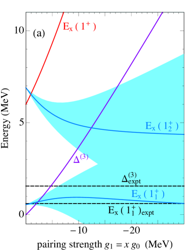
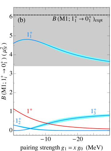
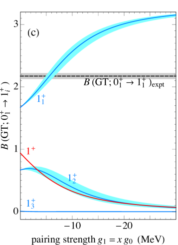
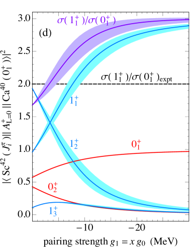
Figure 1: (Color online) Results for (a) excitation energies in ⁴²Sc and the pairing gap $\Delta^{(3)}$, (b) $B({\rm M1};1^{+}_{i}\rightarrow 0^{+}_{1})$ values in ⁴²Sc, (c) $B({\rm GT};0^{+}_{1}\rightarrow 1^{+}_{i})$ strength in the ${}^{42}{\rm Ca}\rightarrow{{}^{42}{\rm Sc}}$ reaction and (d) cross-sections for the ${}^{40}{\rm Ca}\rightarrow{{}^{42}{\rm Sc}}$ reaction. Experimental values are indicated by the black dashed lines with uncertainties in gray. The results of the schematic model are in blue for $T=0$ and in red for $T=1$ states. The calculated pairing gap $\Delta^{(3)}$ in panel (a) and the calculated ratio of cross-sections $\sigma(1^{+}_{1})/\sigma(0^{+}_{1})$ in panel (d) are in purple. All curves are for equal isoscalar and isovector strengths $g_{0}=g_{1}$, and the shaded areas around them are obtained for $g_{0}=g_{1}/x$ with $x$ varying between 0.85 and 1.15.

Results are summarized in Fig. 1. Panel (a) shows the excitation energies of levels in ⁴²Sc (relative to the $0^{+}$ level) as a function of the pairing strengths. The $1^{+}_{1}$ level is at an essentially constant energy for $g_{0}=g_{1}$ but its energy is very sensitive to the ratio of the two pairing strengths. The near-degeneracy of the $(JT)=(01)$ and $(10)$ states, therefore, cannot be used as an indication of Wigner’s SU(4) symmetry in ⁴²Sc, which is only realized in the extreme limit of $g_{0}=g_{1}\gg\Delta\epsilon$. On the other hand, it is to be expected that the isovector pairing strength $g_{1}$ can be constrained from the corresponding observed pairing gap. The “pairing gap” for the odd-mass nucleus ⁴¹Ca, that is, the binding-energy difference

$$\Delta^{(3)}={\frac{1}{2}}\left[{\rm BE}({{}^{42}{\rm Ca}})+{\rm BE}({{}^{40}{\rm Ca}})-2{\rm BE}({{}^{41}{\rm Ca}})\right],$$ (17)

is the only quantity of this kind that is available within our schematic model. Its experimental value of 1.5585 MeV is also shown in panel (a) of Fig. 1 and fixes the isovector pairing strength to $g_{1}\approx-5$ MeV.

Panel (b) shows the $B({\rm M1};1^{+}_{i}\rightarrow 0^{+}_{1})$ values in ⁴²Sc, calculated with a spin quenching factor of 0.74. The M1 strength from the $1^{+}_{1}$ level is known experimentally [9], $B({\rm M1};1^{+}_{1}\rightarrow 0^{+}_{1})=6.1(2.7)$ $\mu_{\rm N}^{2}$, but its error is too large to constrain the pairing strength.

Panel (c) shows the $B({\rm GT};0^{+}_{1}\rightarrow 1^{+}_{i})$ strength for the ⁴²Ca(³He,t)⁴²Sc charge-exchange reaction, using the same quenching factor as in the spin part of the M1 operator. Experimentally, most of the observed strength is concentrated in the $1^{+}$ state at 0.611 MeV [1, 2], which is indicated in the figure, with some fragmentation at higher energies (not shown). This is in qualitative agreement with the schematic model, where the main strength is indeed found in the $1^{+}_{1}$ level with some minor components in two excited $1^{+}$ states with $T=0$ and $T=1$, respectively. Note also that the uncertainty associated with the ratio of pairing strengths is fairly small for the GT strength.

Finally, panel (d) shows results for the ${}^{40}{\rm Ca}\rightarrow{{}^{42}{\rm Sc}}$ np-transfer reaction. We pay particular attention to the ratio of squared amplitudes from Eq. (16) that gives directly the ratio of cross-sections, $\sigma(1^{+}_{1})/\sigma(0^{+}_{1})$. The experimental ratio, $\sim$2, is consistent with our results at the value of the pairing strength $g_{1}$, derived from the $B$(GT) measurement and from the pairing gap $\Delta^{(3)}$. A better agreement would be expected by introducing small admixtures of the $p_{3/2}$ and $p_{1/2}$ orbits, not included in the schematic model. We note here that we have also checked the calculated ratio in the $jj$-coupling scheme by transforming the pair amplitudes into their corresponding $f_{7/2}^{2}$, $f_{5/2}^{2}$ and $f_{7/2}f_{5/2}$ (for $T=0$) components, which were used in DWUCK4 [10] to calculate the cross-sections at forward angles ($L=0$ transfer).

Table 1: Summary of available experimental data [2, 5, 9] and the results of the schematic model for the adopted values of the parameters.

Probe	42Sc level			Experiment	Schematic
	$J^{\pi}$	$E_{\rm x}$ (MeV)			modela
(3He,p)				Relative Intensity
	$0^{+}_{1}$	0		1	1
	$1^{+}_{1}$	0.61		2	2.20(17)
	$(0^{+},1^{+})$	1.89		0.17	—
	$1^{+}$	3.69		1.3	1.57(16)
	$1^{+}$	3.86		0.38	—
(3He,t)				$B$(GT)
	$1^{+}_{1}$	0.61		2.17(5)	2.11(8)
	$1^{+}$	1.89		0.097(3)	—
	$1^{+}$	3.69		0.127(3)	0.62(8)
Lifetime				$B$(M1) ($\mu^{2}_{\rm N}$)
DSAM	$1^{+}_{1}$	0.61		6.1(2.7)	4.80(2)
aThe theoretical uncertainties correspond to a $\pm 15\%$ variation
in the isoscalar pairing strength $g_{0}$, as discussed in the text.

The available experimental data [2, 5, 9] are summarized in Table 1 and compared with the results of the schematic model. The latter are obtained with spin–orbit splitting $\Delta\epsilon=6$ MeV and pairing strengths $g_{0}=g_{1}=-5$ MeV. The isoscalar pairing strength $g_{0}$ is varied by 15% around $g_{1}$ to obtain an estimate of the theoretical uncertainty. Because of the restricted model space with only the $f$ orbital, several observed levels are absent from the theory, as indicated with a dashed line.

Table 2: $LS$-coupling amplitudes (in %) of the yrast $0^{+}$ and $1^{+}$ states of ⁴²Sc, in the schematic model and for the KB3G interaction.

			Schematic model					KB3G ($f^{2}$)
			$L=0$	$L=1$	$L=2$			$L=0$	$L=1$	$L=2$
$0^{+}_{1}$			75	25	—			73	23	—
$1^{+}_{1}$			55	31	14			65	26	4

We can now also study the components in $LS$ coupling of the yrast $0^{+}$ and $1^{+}$ states, for which the schematic model should be reliable. Table 2 lists the amplitudes of $0^{+}_{1}$ and $1^{+}_{1}$, written in the $(LSJT)$ basis of Eqs. (2) and (4). It is seen that the spatially unfavoured components ($L$ odd) are important, which contradicts the assumption of SU(4) symmetry. The fact that nevertheless a strong $B({\rm GT};0^{+}_{1}\rightarrow 1^{+}_{1})$ is observed is due to the constructive addition of the $L=0\rightarrow L=0$ and $L=1\rightarrow L=1$ transitions. Also shown in Table 2 are the corresponding components for the modified Kuo–Brown KB3G Hamiltonian [11], which is a realistic interaction for the entire $pf$ shell [12]. The $f^{2}$ components carry the majority of the strength ($\sim$95%) and the mixing of spatially favoured and unfavoured components is consistent with that found in the schematic model.

In summary, charge-exchange and np-transfer reactions define the elementary modes with isovector and isoscalar pairs that are spatially favoured as well as unfavoured. We have applied this approach to ${}^{40,42}{\rm Ca}\rightarrow{{}^{42}{\rm Sc}}$ reactions to determine the nature of these elementary modes. Good agreement with the experimental data suggests the adequacy of the model. Although the $1^{+}_{1}$ state carries a large fraction of the GT strength, our analysis of both (³He,t) and (³He,p) reactions points out that the SU(4)-symmetry limit is not reached, as the spin–orbit potential breaks the $LS$-coupling scheme. The elementary pairs thus determined can be treated as bosons, leading to an interpretation of GT and np-transfer data in heavier $0f_{7/2}$ nuclei in terms of an interacting boson model—an approach which is currently under study [13]. We believe that this may provide an intuitive and simple picture, which is complementary to state-of-the-art shell-model calculations.

References

- [1] Y. Fujita et al., Phys. Rev. Lett. 112 (2014) 112502.
- [2] Y. Fujita et al., Phys. Rev. C 91 (2015) 064316.
- [3] E. P. Wigner, Phys. Rev. 51 (1937) 106.
- [4] R. W. Zurmühle, C .M. Fou and L. W. Swenson, Nucl. Phys. 80 (1966) 259.
- [5] F. Pühlhofer, Nucl. Phys. 116 (1968) 516.
- [6] J. D. McCullen, B. F. Bayman and L. Zamick, Phys. Rev. 134 (1964) B515.
- [7] N. Zeldes, Phys. Rev. 90 (1953) 416.
- [8] I. Talmi, Simple Models of Complex Nuclei. The Shell Model and the Interacting Boson Model (Harwood, Chur, 1993).
-
[9]
Evaluated Nuclear Structure Data File Database.
http://www.nndc.bnl.gov/ensdf/ -
[10]
P. D. Kunz,
DWUCK4 Program Manual. University of Colorado.
spot.colorado.edu/kunz/DWBA.html - [11] A. Poves, J. Sánchez-Solano, E. Caurier and F. Nowacki, Nucl. Phys. A 694 (2001) 157.
- [12] E. Caurier, G. Martínez-Pinedo, F. Nowacki, A. Poves and A. P. Zuker, Rev. Mod. Phys. 77 (2005) 427.
- [13] P. Van Isacker, to be published.