Abstract

Since 2013, the LHCb collaboration has reported on the measurement of several observables associated to $b\to s$ transitions, finding various deviations from their predicted values in the Standard Model. These include a set of deviations in branching ratios and angular observables, as well as in the observables $R_{K}$ and $R_{K^{\ast}}$, specially built to test the possible violation of Lepton Flavor Universality. Even though these tantalizing hints are not conclusive yet, the $b\to s$ anomalies have gained considerable attention in the flavor community. Here we review New Physics models that address these anomalies and explore their possible connection to the dark matter of the Universe. After discussing some of the ideas introduced in these works and classifying the proposed models, two selected examples are presented in detail in order to illustrate the potential interplay between these two areas of current particle physics.

1 Introduction

The Standard Model (SM) of particle physics provides an excellent description for a vast amount of phenomena and can be regarded as one of the most successful scientific theories ever built. In fact, with the recent discovery of the last missing piece, the Higgs boson, the particle spectrum is finally complete and the SM looks stronger than ever. However, and despite its enormous success, there are several indications that clearly point towards the existence of a more complete theory, with neutrino masses and the baryon asymmetry of the Universe as the most prominent examples.

Another open question is the nature of the dark matter (DM) that accounts for $27\%$ of the energy density of the Universe [1]. Several ideas have been proposed to address this fundamental problem in current physics. Under the hypothesis that the DM is composed of particles, these cannot be identified with any of the states in the SM, hence demanding an extension of the model with new states and, possibly, new dynamics. Again, many directions exist. Interestingly, in scenarios involving New Physics (NP) at the TeV scale, the first signals from the new DM sector might be found in experiments not specially designed to look for them.

Rare decays stand among the most powerful tests of the SM. Since 2013, results obtained by the LHCb collaboration have led to an increasing interest in B physics, particularly in processes involving $b\to s$ transitions. Deviations from the SM expectations have been reported in several observables, some of them hinting at the violation of lepton flavor universality (LFU), a central feature in the SM. Even though these anomalies could be caused by a combination of unfortunate fluctuations and, perhaps, a poor theoretical understanding of some processes, it is tempting to speculate about their possible origin in terms of NP models, in particular models linking them to other open problems.

This mini-review will pursue this goal, focusing on NP scenarios that relate the $b\to s$ anomalies to DM. Several works [2, 3, 4, 5, 6, 7, 8, 9, 10, 11, 12, 13, 14, 15, 16, 17, 18, 19, 20] have already explored this connection, mostly by means of specific models that accommodate the observations in $b\to s$ transitions with a new dark sector. We will review some of the ideas introduced in these works and highlight those that deserve further exploration. We will also classify the proposed models into two general categories: (i) models in which the NP contributions to $b\to s$ transitions and DM production in the early Universe share a common mediator, and (ii) models with the DM particle running in loop diagrams that contribute to the solution of the $b\to s$ anomalies. After a general discussion, a selected example of each class will be presented in detail.

The rest of the manuscript is organized as follows. First, we review the anomalies in $b\to s$ transitions in Sec. 2 and interpret the experimental results in a model independent way in Sec. 3. In Sec. 4 we discuss and classify the proposed New Physics explanations to these anomalies that involve a link to the dark matter problem. Secs. 5 and 6 present two simple example models that illustrate this connection. Finally, we summarize and draw our conclusions in Sec. 7.

2 Experimental situation

We begin by discussing the present experimental situation. The observed anomalies in $b\to s$ transitions can be classified into two classes: (1) branching ratios and angular observables, and (2) lepton flavor universality violating (LFUV) anomalies. Although they might be related (and caused by the same NP), they are conceptually different.

Branching ratios and angular observables: using state-of-the-art computations of the hadronic form factors involved, one can compute branching ratios and angular observables for $b\to s$ processes such as $B\to K^{\ast}\ell^{+}\ell^{-}$ and look for deviations from the SM predictions. For the comparison to be meaningful, one must have a good knowledge of all possible Quantum ChromoDynamics (QCD) effects that might pollute the theoretical calculation and we currently have at our disposal several methods to minimize or at least estimate the uncertainties.  In particular, a basis of optimized observables for the decay $B\to K^{\ast}\mu^{+}\mu^{-}$, specially designed to reduce the hadronic uncertainties, was introduced in [29]. In 2013, the LHCb collaboration published results on these observables using their $1$ fb^-1 dataset, finding a $3.7\sigma$ deviation between the measurement and the SM prediction for the $P_{5}^{\prime}$ angular observable in one dimuon invariant mass bin [30]. A systematic deficit with respect to the SM predictions in the branching ratios of several processes, mainly $B_{s}\to\phi\mu^{+}\mu^{-}$, was also reported by LHCb [31]. These discrepancies have been found later in other datasets. In 2015, LHCb confirmed these anomalies using their full Run 1 dataset with $3$ fb^-1 [32, 33], whereas in 2016 the Belle collaboration presented an independent measurement of $P_{5}^{\prime}$, compatible with the LHCb result [34, 35]. More recently, both ATLAS [36] and CMS [37] have also presented preliminary results on the $B\to K^{\ast}\mu^{+}\mu^{-}$ angular observables, with relatively good agreement with LHCb.

LFUV anomalies: one of the central features of the SM is that gauge bosons couple with the same strength to all three families of leptons. This prediction can be tested by measuring observables such as the $R_{K^{(\ast)}}$ ratios, defined as [38]

$$R_{K^{(\ast)}}=\frac{\Gamma(B\rightarrow K^{(\ast)}\mu^{+}\mu^{-})}{\Gamma(B\rightarrow K^{(\ast)}e^{+}e^{-})}\,,$$ (1)

measured in specific dilepton invariant mass squared ranges $q^{2}\in[q^{2}_{\rm min},q^{2}_{\rm max}]$. In the SM, these ratios should be very approximately equal to one. Furthermore, hadronic uncertainties are expected to cancel to very good approximation in these ratios, which implies that, in contrast to the previous class of anomalies, deviations in these observables cannot be explained by uncontrolled QCD effects and would be a clear indication of NP at work. For this reason, they are sometimes referred to as clean observables. Interestingly, in 2014 the LHCb collaboration measured $R_{K}$ in the region $[1,6]$ GeV² [39], finding a value significantly lower than one, while in 2017 similar measurements of the $R_{K^{\ast}}$ ratio in two $q^{2}$ bins [40] were also found to depart from their SM expected values:

$$R_{K} =0.745^{+0.090}_{-0.074}\pm 0.036\,,\quad q^{2}\in[1,6]~{}\text{GeV}^{2}\,,$$

$$R_{K^{\ast}} =0.660^{+0.110}_{-0.070}\pm 0.024\,,\quad q^{2}\in[0.045,1.1]~{}\text{GeV}^{2}\,,$$

$$R_{K^{\ast}} =0.685^{+0.113}_{-0.069}\pm 0.047\,,\quad q^{2}\in[1.1,6.0]~{}\text{GeV}^{2}\,.$$ (2)

The comparison between these experimental results and the SM predictions [41, 42],

$$R_{K}^{\rm{SM}} =1.00\pm 0.01\,,\quad q^{2}\in[1,6]~{}\text{GeV}^{2}\,,$$

$$R_{K^{\ast}}^{\rm{SM}} =0.92\pm 0.02\,,\quad q^{2}\in[0.045,1.1]~{}\text{GeV}^{2}\,,$$

$$R_{K^{\ast}}^{\rm{SM}} =1.00\pm 0.01\,,\quad q^{2}\in[1.1,6.0]~{}\text{GeV}^{2}\,,$$ (3)

shows deviations from the SM at the $2.6\,\sigma$ level in the case of $R_{K}$, $2.2\,\sigma$ for $R_{K^{\ast}}$ in the low-$q^{2}$ region, and $2.4\,\sigma$ for $R_{K^{\ast}}$ in the central-$q^{2}$ region. Finally, Belle has recently measured the LFUV observable $Q_{5}=P_{5}^{\mu\,\prime}-P_{5}^{e\,\prime}$, with the observable $P_{5}^{e\,\prime}$ defined for $B\to K^{\ast}e^{+}e^{-}$ analogously to $P_{5}^{\mu\,\prime}\equiv P_{5}^{\prime}$ for $B\to K^{\ast}\mu^{+}\mu^{-}$ [43]. The result, although statistically not very significant, also points towards the violation of LFU [35].

Summarizing, there are at present two sets of experimental anomalies in processes involving $b\to s$ transitions at the quark level. While the relevance of the first set is currently a matter of discussion due to the possibility of unknown QCD effects faking the deviations from the SM, the second can only be explained by NP violating LFU. In principle, these two classes of anomalies can be completely unrelated but, as we will see in the next Section, global analyses of all experimental data in $b\to s$ transitions indicate that a common explanation (in terms of a single effective operator) can address both sets in a satisfactory and economical way. This intriguing result has made the $b\to s$ anomalies a topic of great interest currently.

Finally, it is very interesting to note the existence of an independent set of anomalies in $b\to c$ transitions. Several experimental measurements of the ratios $R(D)$ and $R(D^{\ast})$ have been found to depart from their SM predictions, with a global discrepancy at the $\sim 4\sigma$ level [44]. Recently, the $R(J/\psi)$ ratio has also been measured by the LHCb collaboration, finding again a deviation from the SM expected value [45]. Compared to the $b\to s$ anomalies, the $b\to c$ anomalies are of a different nature and, if real, they could have a completely different origin. For instance, they would involve a new charged current, instead of a neutral one, hence requiring the new mediators to be much lighter to be able to compete with the SM $W$ boson tree-level exchange. However, many authors have proposed models that can simultaneously address both sets of anomalies. We refer to [46] for a general discussion on combined explanations and ignore the $b\to c$ anomalies for the rest of this paper.

3 Model independent interpretation

The experimental tensions discussed in the previous Section must be properly quantified and interpreted. Quantification is crucial to determine whether the anomalies can be explained by fluctuations in the data or they truly indicate a statistically significant deviation from the SM. Assuming that these tensions are caused by genuine NP, the ultimate goal is to construct a specific model in which they are solved. However, the first step in this direction must be a model independent interpretation of the experimental data in order to identify the ingredients that this new scenario must include. This is achieved by adopting an approach based on effective operators, valid under the assumption that all NP degrees of freedom lie at energies well above the relevant energy scales for the observables of interest.

The effective Hamiltonian for $b\to s$ transitions is usually written as

$$\mathcal{H}_{\text{eff}}=-\frac{4G_{F}}{\sqrt{2}}\,V_{tb}V_{ts}^{\ast}\,\frac{e^{2}}{16\pi^{2}}\,\sum_{i}\left(C_{i}\,\mathcal{O}_{i}+C^{\prime}_{i}\,\mathcal{O}^{\prime}_{i}\right)+\text{h.c.}\,.$$ (4)

Here $G_{F}$ is the Fermi constant, $e$ the electric charge and $V$ the Cabibbo-Kobayashi-Maskawa (CKM) matrix. $\mathcal{O}_{i}$ and $\mathcal{O}^{\prime}_{i}$ are the effective operators that contribute to $b\to s$ transitions, and $C_{i}$ and $C^{\prime}_{i}$ their Wilson coefficients. The most relevant operators for the interpretation of the $b\to s$ anomalies are

$$\mathcal{O}_{9} =\left(\bar{s}\gamma_{\mu}P_{L}b\right)\,\left(\bar{\ell}\gamma^{\mu}\ell\right)\,, \mathcal{O}^{\prime}_{9} =\left(\bar{s}\gamma_{\mu}P_{R}b\right)\,\left(\bar{\ell}\gamma^{\mu}\ell\right)\,,$$ (5)

$$\mathcal{O}_{10} =\left(\bar{s}\gamma_{\mu}P_{L}b\right)\,\left(\bar{\ell}\gamma^{\mu}\gamma_{5}\ell\right)\,, \mathcal{O}^{\prime}_{10} =\left(\bar{s}\gamma_{\mu}P_{R}b\right)\,\left(\bar{\ell}\gamma^{\mu}\gamma_{5}\ell\right)\,.$$ (6)

Here $\ell=e,\mu,\tau$. In fact, the operators and Wilson coefficients carry flavor indices and we are omitting them to simplify the notation. When necessary, we will denote a particular lepton flavor with a superscript, e.g. $C_{9}^{\mu}$ and $\mathcal{O}_{9}^{\mu}$, for muons. It is also convenient to split the Wilson coefficients in two pieces: the SM contributions and the NP contributions, defining 

$$C_{9} = C_{9}^{\text{SM}}+C_{9}^{\text{NP}}\,,$$ (7)

$$C_{10} = C_{10}^{\text{SM}}+C_{10}^{\text{NP}}\,.$$ (8)

The SM contributions have been computed at NNLO at $\mu_{b}=4.8$ GeV, obtaining $C_{9}^{\text{SM}}(\mu_{b})=4.07$ and $C_{10}^{\text{SM}}(\mu_{b})=-4.31$ (see [29] and references therein), leaving the NP contributions as parameters to be determined (or at least constrained) by using experimental data.

It is in principle possible to derive limits for the NP contributions considering each observable independently, but this approach would completely miss the global picture. The effective operators in Eq. (4) contribute to several observables and one expects the presence of NP to be revealed by a pattern of deviations from the SM expectations, rather than by a single anomaly. For this reason, global fits constitute the best approach to analyze the available experimental data. Interestingly, several independent fits [47, 48, 49, 50, 51, 52, 53, 54] have found a remarkable tension between the SM and experimental data on $b\to s$ transitions which is clearly reduced with the addition of NP contributions. Although the numerical details (such as statistical significances) differ among different analyses, there is a general consensus on the following qualitative results:

• Global fits improve substantially with a negative contribution in $C_{9}^{\mu,\text{NP}}$, with $C_{9}^{\mu,\text{NP}}\sim-25\%\times C_{9}^{\mu,\text{SM}}$, leading to a total Wilson coefficient $C_{9}^{\mu}$ significantly smaller than the one in the SM.

• NP contributions in other Wilson coefficients can also improve the fit, but only in a sub-dominant way. For instance, the anomalies can also be accommodated in scenarios with $C_{9}^{\mu,\text{NP}}=-C_{10}^{\mu,\text{NP}}$ or $C_{9}^{\mu,\text{NP}}=-C_{9}^{\prime\>\mu,\text{NP}}$, without a clear statistical preference with respect to the scenario with NP only in $C_{9}^{\mu}$. 

• Other operators involving muons are perfectly compatible with their SM values. Similarly, no NP is required for operators involving electrons or tau leptons.

Armed with these results, model builders can construct specific models where all requirements are met and the anomalies explained. Similarly, one can extract interesting implications for model building by explaining the anomalies in terms of gauge invariant effective operators, see [55] for a recent analysis. Either way, the resulting profile of NP contributions reveals a pattern that was not predicted by any theoretical framework, such as supersymmetry, and many new models have been put forward. In the next Section we will discuss some of these models, in particular those linking the $b\to s$ anomalies to dark matter.

4 Linking the $\boldsymbol{b\to s}$ anomalies to dark matter

After discussing the current experimental situation in $b\to s$ transitions, let us focus on possible connections to the dark matter problem. These have been explored in [2, 3, 4, 5, 6, 7, 8, 9, 10, 11, 12, 13, 14, 15, 16, 17, 18, 19, 20]. In general, the proposed models that solve the $b\to s$ anomalies and explain the origin of the dark matter of the Universe can be classified into two principal categories:

• Portal models: models in which the mediator responsible for the NP contributions to $b\to s$ transitions also mediates the DM production in the early Universe.

• Loop models: models that induce the required NP contributions to $b\to s$ transitions with loops containing the DM particle.

In the case of portal models, the usual scenario considers a $U(1)$ gauge extension of the SM that leads to the existence of a new massive gauge boson after spontaneous symmetry breaking. The resulting $Z^{\prime}$ boson induces a new neutral current contribution in $b\to s$ transitions and mediates the production of DM particles in the early Universe via a $Z^{\prime}$ portal interaction. This setup was first considered in [2]. In this particular realization of the general idea, the SM fermions were assumed to be neutral under the new $U(1)_{X}$ gauge symmetry and the $Z^{\prime}$ couplings to quarks ($\overline{b}s$) and leptons ($\mu^{+}\mu^{-}$), necessary to explain the $b\to s$ anomalies, are generated at tree-level via mixing with new vector-like (VL) fermions. Additionally, the $Z^{\prime}$ boson also couples to the scalar field $\chi$, the DM candidate in this model, automatically stabilized by an remnant $\mathbb{Z}_{2}$ symmetry after $U(1)_{X}$ breaking. This model will be reviewed in more detail in Sec. 5. Variants of this setup with fermionic DM also exist. In [6], a horizontal $U(1)_{B_{1}+B_{2}-2B_{3}}$ gauge symmetry is introduced, with $B_{i}$ the baryon number of the ith fermion family. The resulting $Z^{\prime}$ boson couples directly to the SM quarks, while the coupling to muons is obtained by introducing a VL lepton. This allows to accommodate the anomalies in $b\to s$ transitions. Furthermore, the model also contains a Dirac fermion that is stable due to a remnant $\mathbb{Z}_{2}$ symmetry, in a similar fashion as in [2], which becomes the DM candidate. Similarly, Ref. [7] builds on the well-known $U(1)_{L_{\mu}-L_{\tau}}$ model of [56] and extends it to include a stable Dirac fermion with a relic density also determined by $Z^{\prime}$ portal interactions, while [20] considers a similar model but makes use of kinetic mixing between the $Z^{\prime}$ and the SM neutral gauge bosons. Ref. [19] considers vector-like neutrino DM in a setup analogous to [2] extended with additional VL fermions. Ref. [10] explored a pair of scenarios based on a $U(1)$ gauge symmetry supplemented with VL fermions and a fermionic DM candidate, of Dirac or Majorana nature. This paper focuses on effects in indirect detection experiments, aiming at an explanation of the excess of events in antiproton spectra reported by the AMS-02 experiment in 2016 [57]. Other works that adopt the standard $Z^{\prime}$ portal setup are [4, 12]. Finally, [11] considers a light mediator (not the usual heavy $Z^{\prime}$) that contributes to $b\to s$ transitions and decays predominantly into invisible final states, possibly made of light DM particles.

It is important to note that the phenomenology of these $Z^{\prime}$ portal models differs substantially from the standard $Z^{\prime}$ portal phenomenology. This is due to the fact that the $Z^{\prime}$ bosons in these models couple with different strengths to different fermion families, as required to accommodate the LFUV hints observed by the LHCb collaboration ($R_{K}$ and $R_{K^{\ast}}$). For instance, DM annihilation typically yields muon and tau lepton pairs, but not electrons and positrons. Direct detection experiments are also more challenging that in the standard $Z^{\prime}$ portal scenario, since the DM candidate typically does not couple to first generation quarks, more abundant in the nucleons.

In what concerns loop models, many variations are possible. To the best of our knowledge, the first model of this type that appeared in the literature is [13], based on previous work on loop models for the $b\to s$ anomalies, without connecting to the DM problem, in [58, 59]. In this model the SM particle content is extended with two VL pairs of $SU(2)_{L}$ doublets, with the same quantum numbers as the SM quark and lepton doublets, but charged under a global $U(1)_{X}$ symmetry. The model also contains the complex scalar $X$, singlet under the SM gauge symmetry and also charged under $U(1)_{X}$. With these states, one can draw a 1-loop diagram contributing to the $b\to s$ observables relevant to explain the anomalies. Furthermore, if the global $U(1)_{X}$ is conserved, the lightest $U(1)_{X}$-charged state becomes stable. In this work, this state is assumed to be $X$, hence the DM candidate in the model. A more detail discussion about this model can be found in Sec. 6. Two similar setups can be found in [18], where a different set of global symmetries are considered ($U(1)\times\mathbb{Z}_{2}$ and $U(1)\times\mathbb{Z}_{3}$) in order to stabilize a scalar DM candidate. This paper also includes right-handed neutrinos in order to accommodate non-zero neutrino masses with the type-I seesaw mechanism and explores the lepton flavor violating phenomenology of the model in detail. A Majorana fermionic DM candidate was considered in [16]. Similarly to the previously mentioned models, this scenario also addresses the $b\to s$ anomalies at 1-loop level introducing a minimal number of fields: just a VL quark ($\Psi$) and an inert scalar doublet ($\Phi$), in addition to the fermion singlet that constitutes the DM candidate. The model is supplemented with a discrete $\mathbb{Z}_{2}$ symmetry to ensure the stability of the DM particle. Interestingly, the model can be tested in direct DM detection experiments as well as at the Large Hadron Collider (LHC), where the states $\Psi$ and $\Phi$ can be pair-produced and lead to final states with hard leptons and missing energy. Finally, an extended loop model for the $b\to s$ anomalies which also has an additional $U(1)$ gauge symmetry, contains a scalar DM candidate and explains neutrino masses can be found in [17].

Finally, let us comment on other models and works that do not easily fit within any of the two categories mentioned above. The model in [3] is very similar to the model in [2]. It also extends the SM with a complex scalar, VL quarks and leptons and a new $U(1)_{X}$ gauge symmetry that breaks down to a $\mathbb{Z}_{2}$ parity. However, the VL leptons carry different $U(1)_{X}$ charges, leading to a loop-induced $Z^{\prime}\mu^{+}\mu^{-}$ coupling. This changes the DM phenomenology dramatically. The dominant mechanism for the DM production in the early Universe is not a $Z^{\prime}$ portal interaction, but t-channel exchange of VL leptons. The model in [9] can be regarded as a hybrid model, with features from both portal and loop models. The SM symmetry group is extended with a new $U(1)_{\mu-\tau}\times\mathbb{Z}_{2}$ piece. The first factor leads to the existence of a massive $Z^{\prime}$ boson while the second one stabilizes a scalar DM candidate. The $Z^{\prime}\overline{b}s$ coupling is generated with a loop containing the $\mathbb{Z}_{2}$-odd fields and the dominant DM production mechanism is a $Z^{\prime}$ portal interaction, mainly with leptons. The $Z^{\prime}\overline{b}s$ coupling is also loop-generated in [14], but in this case production of DM particles takes place via a Higgs portal. [8] proposes an extended Scotogenic model for neutrino masses [60] supplemented with a non-universal $U(1)$ gauge group. The DM candidate in this case is the lightest fermion singlet and is produced by Yukawa interactions. Finally, two models that address the $b\to s$ anomalies with leptoquarks and include DM candidates were introduced in [5] and [15]. In the former the DM candidate is a component of an $SU(2)_{L}$ multiplet introduced to enhance the diphoton rate of a scalar in the model, whereas in the latter the DM candidate is a baryon-like composite state in a model with strong dynamics at the TeV scale.

Having reviewed and classified the proposed models, we now proceed to discuss in some detail two specific examples. These illustrate the main features of portal and loop models.

5 An example portal model

We will now review the model introduced in [2], arguably one of the simplest scenarios to account for the $b\to s$ anomalies with a dark sector. Some of the ingredients of this model were already present in the model of [56], which is extended in the quark sector (following the same lines as in the lepton sector). It also includes a dark matter candidate that couples to the SM fields via the same mediator that leads to an explanation to the $b\to s$ anomalies, a heavy $Z^{\prime}$ boson. A variation of this scenario with a loop-induced coupling to muons appeared afterwards in [3], whereas the phenomenology of an extension to account for neutrino masses is discussed in [61].

Field	Group	Coupling
$B$	$U(1)_{Y}$	$g_{1}$
$W$	$SU(2)_{L}$	$g_{2}$
$g$	$SU(3)_{c}$	$g_{3}$
$B_{X}$	$U(1)_{X}$	$g_{X}$

Table 1: Gauge sector of the model of [2].

Field	Spin	$SU(3)_{c}\times\,SU(2)_{L}\times\,U(1)_{Y}\times U(1)_{X}$
$\phi$	$0$	$({\bf 1},{\bf 1},0,2)$
$\chi$	$0$	$({\bf 1},{\bf 1},0,-1)$
$Q_{L,R}$	$\frac{1}{2}$	$({\bf 3},{\bf 2},\frac{1}{6},2)$
$L_{L,R}$	$\frac{1}{2}$	$({\bf 1},{\bf 2},-\frac{1}{2},2)$

Table 2: New scalars and fermions in the model of [2].

The model extends the SM gauge group with a new dark $U(1)_{X}$ factor, under which all the SM particles are assumed to be singlets. The dark sector contains two pairs of vector-like fermions, $Q$ and $L$, as well as the complex scalar fields, $\phi$ and $\chi$. Tables 1 and 2 show all the details about the gauge sector and the new scalars and fermions in the model. $Q$ and $L$ have the same representation under the SM gauge group as the SM doublets $q$ and $\ell$, and they can be decomposed under $SU(2)_{L}$ as

$$Q_{L,R}=\left(\begin{array}[]{c}U\\ D\end{array}\right)_{L,R}\quad,\quad L_{L,R}=\left(\begin{array}[]{c}N\\ E\end{array}\right)_{L,R}\,,$$ (9)

with the electric charges of $U$, $D$, $N$ and $E$ being $+2/3$, $-1/3$, $0$ and $-1$, respectively. In contrast to their SM counterparts, $Q$ and $L$ are vector-like fermions charged under the dark $U(1)_{X}$. In addition to the usual canonical kinetic terms, the new vector-like fermions $Q$ and $L$ have Dirac mass terms,

$$\mathcal{L}_{m}=m_{Q}\,\overline{Q}Q+m_{L}\,\overline{L}L\,,$$ (10)

as well as Yukawa couplings with the SM doublets $q$ and $\ell$ and the scalar $\phi$,

$$\mathcal{L}_{Y}=\lambda_{Q}\,\overline{Q_{R}}\,\phi\,q_{L}+\lambda_{L}\,\overline{L_{R}}\,\phi\,\ell_{L}+\text{h.c.}\,,$$ (11)

where $\lambda_{Q}$ and $\lambda_{L}$ are $3$ component vectors. The scalar potential of the model can be split into different pieces,

$$\mathcal{V}=\mathcal{V}_{\text{SM}}+\mathcal{V}\left(H,\phi,\chi\right)+\mathcal{V}\left(\phi,\chi\right)\,.$$ (12)

$\mathcal{V}_{\text{SM}}$ is the usual SM scalar potential containing quadratic and quartic terms for the Higgs doublet $H$. The new terms involving the scalars $\phi$ and $\chi$ are

$$\mathcal{V}\left(H,\phi,\chi\right)=\lambda_{H\phi}\,|H|^{2}|\phi|^{2}+\lambda_{H\chi}\,|H|^{2}|\chi|^{2}$$ (13)

and

$$\mathcal{V}\left(\phi,\chi\right)=m_{\phi}^{2}|\phi|^{2}+m_{\chi}^{2}|\chi|^{2}+\frac{\lambda_{\phi}}{2}|\phi|^{4}+\frac{\lambda_{\chi}}{2}|\chi|^{4}+\lambda_{\phi\chi}\,|\phi|^{2}|\chi|^{2}+\left(\mu\,\phi\chi^{2}+\text{h.c.}\right)\,.$$ (14)

All $\lambda_{i}$ couplings are dimensionless, whereas $\mu$ has dimensions of mass and $m_{\phi}^{2}$ and $m_{\chi}^{2}$ have dimensions of mass². We will assume that the scalar potential parameters allow for the vacuum configuration

$$\langle H^{0}\rangle=\frac{v}{\sqrt{2}}\qquad,\qquad\langle\phi\rangle=\frac{v_{\phi}}{\sqrt{2}}\,,$$ (15)

where $H^{0}$ is the neutral component of the Higgs doublet $H$. The scalar $\chi$ does not get a vacuum expectation value (VEV). Therefore, the scalar $\phi$ will be responsible for the spontaneous breaking of $U(1)_{X}$. This automatically leads to the existence of a new massive gauge boson, the $Z^{\prime}$ boson, with mass $m_{Z^{\prime}}=2g_{X}v_{\phi}$. In the absence of mixing between the $U(1)$ gauge bosons, the $Z^{\prime}$ boson can be identified with the original $B_{X}$ boson in Table 1. We note that a Lagrangian term of the form $\mathcal{L}\supset\varepsilon\,F_{\mu\nu}^{Y}F^{\mu\nu}_{X}$, where $F_{\mu\nu}^{X,Y}$ are the usual field strength tensors for the $U(1)_{X,Y}$ groups, would induce this mixing. In order to avoid phenomenological difficulties associated to this mixing we will assume that $\varepsilon\ll 1$. Moreover, it can be shown that loop contributions to this mixing are kept under control if $m_{Q}\simeq m_{L}$ [2].

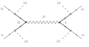
Figure 1: Generation of $\mathcal{O}_{9}$ and $\mathcal{O}_{10}$ in the model of [2]. The mixing between the SM fermions and the vector-like ones induce semileptonic four-fermion interactions.

Let us now discuss how this model solves the $\boldsymbol{b\to s}$ anomalies. After the spontaneous breaking of $U(1)_{X}$, the Yukawa interactions in Eq. (11) lead to mixings between the vector-like fermions and their SM counterparts. This mixing results in $Z^{\prime}$ effective couplings to the SM fermions. If these are parametrized as [62, 63]

$$\mathcal{L}\supset\bar{f}_{i}\gamma^{\mu}\left(\Delta_{L}^{f_{i}f_{j}}P_{L}+\Delta_{R}^{f_{i}f_{j}}P_{R}\right)f_{j}Z_{\mu}^{\prime}\,,$$ (16)

and one assumes $\lambda_{Q}^{d}=\lambda_{L}^{e}=\lambda_{L}^{\tau}=0$ for the sake of simplicity, the $Z^{\prime}$ couplings to $\overline{b}s$ and $\mu^{+}\mu^{-}$, necessary to solve the $b\to s$ anomalies, are found to be

$$\Delta_{L}^{bs}=\frac{2\,g_{X}\lambda_{Q}^{b}\lambda_{Q}^{s\ast}v_{\phi}^{2}}{2m_{Q}^{2}+\left(|\lambda_{Q}^{s}|^{2}+|\lambda_{Q}^{b}|^{2}\right)v_{\phi}^{2}}\quad,\quad\Delta_{L}^{\mu\mu}=\frac{2\,g_{X}|\lambda_{L}^{\mu}|^{2}v_{\phi}^{2}}{2m_{L}^{2}+|\lambda_{L}^{\mu}|^{2}v_{\phi}^{2}}\,.$$ (17)

These couplings induce a tree-level contribution to the semileptonic four-fermion operators in Eqs. (5) and (6), as shown esquematically in Fig. 1. More specifically, given that the SM fermions participating in the effective vertices are left-handed, see Eq. (11), the operators $\mathcal{O}_{9}$ and $\mathcal{O}_{10}$ are generated simultaneously, with [63]

$$C_{9}^{\mu,\text{NP}}=-C_{10}^{\mu,\text{NP}}=-\frac{\Delta_{L}^{bs}\Delta_{L}^{\mu\mu}}{V_{tb}V_{ts}^{\ast}}\,\left(\frac{\Lambda_{v}}{m_{Z^{\prime}}}\right)^{2}\,,$$ (18)

where we have introduced

$$\Lambda_{v}=\left(\frac{\pi}{\sqrt{2}G_{F}\alpha}\right)^{1/2}\simeq 4.94\,\text{TeV}\,,$$ (19)

with $\alpha=\frac{e^{2}}{4\pi}$ the electromagnetic fine structure constant. $\Lambda_{v}$ and the CKM elements appear in Eq. (18) in order to normalize the Wilson coefficients as defined in Eqs. (5) and (6). By taking proper ranges for the model parameters, the required values for these Wilson coefficients, previously identified by the global fits to flavor data, can be easily obtained.

Finally, we move to the discussion on the Dark Matter phenomenology of the model. We note that the model does not include any ad-hoc stabilizing symmetry for the DM candidate $\chi$. However, this state is perfectly stable. This is due to the fact that the continuous $U(1)_{X}$ symmetry leaves a remnant $\mathbb{Z}_{2}$ parity, under which $\chi$ is odd, after spontaneous symmetry breaking [64, 65, 66]. Therefore, the same symmetry that leads to the dynamics behind the $b\to s$ anomalies is also at the origin of the DM stabilization mechanism. Furthermore, the DM production in the early Universe can take place via $2\leftrightarrow 2$ processes mediated by the $Z^{\prime}$ boson, thus establishing another link with the $b\to s$ anomalies. Indeed, purely gauge interactions open a $Z^{\prime}$ portal that induces $\bar{F}F\leftrightarrow\chi\chi^{*}$ annihilation processes, with $F=q,\ell,Q,L$, as shown in Fig. 2.  We notice that these processes match those in Fig. 1 if one trades one of the fermion pairs for $\chi\chi^{*}$. Therefore, one can establish an interplay between flavor and DM physics in this scenario. Fig. 3 illustrates this connection displaying contours for constant $\log(\Omega_{\text{DM}}h^{2})$ (the DM relic density) and the ratio $C_{9}^{\mu,\text{NP}}/C_{9}^{\mu,\text{SM}}$ in the $(g_{X},m_{Z^{\prime}})$ plane. This figure has been obtained with fixed $\lambda_{Q}^{b}=\lambda_{Q}^{s}=0.025$, $\lambda_{L}^{\mu}=0.5$, $m_{Q}=m_{L}=1~{}\text{TeV}$ and $m^{2}_{\chi}=1~{}\text{TeV}^{2}$. The calculation of the flavor observables has been performed with FlavorKit [67], whereas the DM relic density has been evaluated with MicrOmegas [68]. We see that there is a region in parameter space, with moderately large $g_{X}\simeq 0.3$, where the observed DM relic density can be reproduced and a ratio $C_{9}^{\mu,\text{NP}}/C_{9}^{\mu,\text{SM}}$ in agreement with the global fits is obtained. We also note that the DM relic density tends to be large. In fact, in order to obtain a numerical value in the ballpark of $\Omega_{\rm DM}h^{2}\simeq 0.1$ one has to be rather close to the resonant region with $m_{Z^{\prime}}\simeq 2\,m_{\chi}$, which in this plot is located around $m_{Z^{\prime}}=2$ TeV.

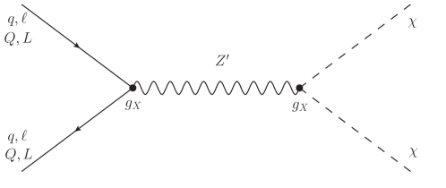
Figure 2: DM production via the $Z^{\prime}$ portal in the model of [2]. We notice that the vertex on the left of the diagram also participates in the explanation of the $b\to s$ anomalies (see Fig.1).

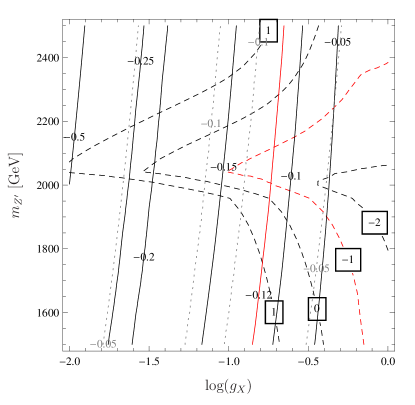
Figure 3: Contours for constant $C_{9}^{\mu,\text{NP}}/C_{9}^{\mu,\text{SM}}$ and $\log(\Omega_{\text{DM}}h^{2})$ (dashed black) in the $(g_{X},m_{Z^{\prime}})$ plane. For the ratio $C_{9}^{\mu,\text{NP}}/C_{9}^{\mu,\text{SM}}$ the full 1-loop results are shown via the black lines, while the dotted grey lines give the values using the tree-level approximation. Red lines indicate the preferred values for $C_{9}^{\mu,\text{NP}}/C_{9}^{\mu,\text{SM}}$ and $\log(\Omega_{\text{DM}}h^{2})$ from global fits and cosmological observations, respectively. Figure taken from [2].

Besides flavor and DM physics, the model has rich phenomenological prospects in other fronts. The new states can be discovered at the LHC in large portions of the parameter space. Although one typically assumes that the $Z^{\prime}$ boson couples predominantly to the second and third generation quarks ($|\lambda_{Q}^{d}|\ll 1$), the resulting suppressed production cross-sections at the LHC can still be sufficient for a discovery, see for instance [69]. Furthermore, the new VL fermions can also be produced and detected. In particular, the heavy VL quarks masses are already pushed beyond the TeV scale due to their efficient production in $pp$ collisions. In what concerns direct and indirect DM detection, scenarios with a dark $Z^{\prime}$ portal have been discussed in [70, 71]. For more details about this model, its predictions and the most relevant experimental constraints we refer to [2].

6 An example loop model

We now turn our attention to the second class of models, those that explain the $b\to s$ anomalies via loop diagrams including DM particles. A simple but illustrative example of this category is that presented in [13]. Previous work on loop models for the $b\to s$ anomalies, without connecting to the DM problem, can be found in [58, 59].

Field	Spin	$SU(3)_{c}\times\,SU(2)_{L}\times\,U(1)_{Y}$	$U(1)_{X}$
$X$	$0$	$({\bf 1},{\bf 1},0)$	$-1$
$Q_{L,R}$	$\frac{1}{2}$	$({\bf 3},{\bf 2},\frac{1}{6})$	$\phantom{+}1$
$L_{L,R}$	$\frac{1}{2}$	$({\bf 1},{\bf 2},-\frac{1}{2})$	$\phantom{+}1$

Table 3: New scalars and fermions in the model of [13]. The $U(1)_{X}$ symmetry is global.

The model introduces two VL fermions, $Q$ and $L$, with the same gauge quantum numbers as the SM quark and lepton doublets, respectively. It also adds the complex scalar $X$, a complete singlet under the SM gauge symmetry. The new fields are charged under a global Abelian symmetry, $U(1)_{X}$, under which all SM fields are assumed to be singlets. As we will see below, this particle content is sufficient to address the $b\to s$ anomalies. Table 3 details the new fields and their charges under the gauge and global symmetries of the model.

The VL fermions $Q$ and $L$ can be decomposed as in Eq. (9), with their $SU(2)_{L}$ components having exactly the same electric charges as in that case. Therefore, the same Dirac mass terms as in Eq. (10) can be written. In addition, the symmetries of the model allow for the Yukawa couplings with the SM doublets $q$ and $\ell$ and the scalar $X$

$$\mathcal{L}_{Y}=\lambda_{Q}\,\overline{Q_{R}}\,X\,q_{L}+\lambda_{L}\,\overline{L_{R}}\,X\,\ell_{L}+\text{h.c.}\,,$$ (20)

where $\lambda_{Q}$ and $\lambda_{L}$ are $3$ component vectors. The scalar potential of the model contains the following terms

$$\mathcal{V}=\mathcal{V}_{\text{SM}}+m_{X}^{2}|X|^{2}+\lambda_{X}\,|X|^{4}+\lambda_{H}\,|H|^{2}|X|^{2}\,.$$ (21)

All $\lambda_{i}$ couplings are dimensionless, whereas $m_{X}^{2}$ has dimensions of mass². In the following, possible effects due to the $\lambda_{H}$ coupling will be ignored, assuming $\lambda_{H}\ll 1$. We will also assume that the scalar potential parameters allow for a vacuum configuration with $\langle X\rangle=0$. In this case, the global $U(1)_{X}$ symmetry is conserved and the lightest state with a non-vanishing charge under this symmetry is completely stable. Moreover, we note that the conservation of $U(1)_{X}$ prevents the VL fermions from mixing with the SM ones.

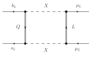
Figure 4: Generation of $\mathcal{O}_{9}$ and $\mathcal{O}_{10}$ in the model of [13]. Semileptonic four-fermion operators are generated at the 1-loop level.

We move now to the solution of the $\boldsymbol{b\to s}$ anomalies in the context of this model. It is straightforward to check that no NP contributions to $b\to s$ transitions are generated at tree-level in this model.  However, the semileptonic operators $\mathcal{O}_{9}$ and $\mathcal{O}_{10}$ are generated at the 1-loop level as shown in Fig. 4. This diagram leads to

$$C_{9}^{\mu,\text{NP}}=-C_{10}^{\mu,\text{NP}}=\frac{\lambda_{Q}^{b}\lambda_{Q}^{s\ast}|\lambda_{L}^{\mu}|^{2}}{64\,\pi^{2}\,V_{tb}V_{ts}^{\ast}}\,\frac{\Lambda_{v}^{2}}{m_{Q}^{2}-m_{L}^{2}}\,\left[f\left(\frac{m_{X}^{2}}{m_{Q}^{2}}\right)-f\left(\frac{m_{X}^{2}}{m_{L}^{2}}\right)\right]\,,$$ (22)

where $\Lambda_{v}$ was introduced in Eq. (19) and $f(x)$ is the loop function

$$f(x)=\frac{1}{x-1}-\frac{\ln x}{(x-1)^{2}}\,.$$ (23)

This loop-level solution to the $b\to s$ anomalies corresponds to scenario A-I, model class b), in [59]. Fig. 5 shows that the model can accommodate the $R_{K}$ and $R_{K^{\ast}}$ measurements by the LHCb collaboration. This figure has been obtained with fixed $|\lambda_{Q}^{b}\lambda_{Q}^{s}|=0.15$, $m_{L}=1$ TeV and $m_{Q}=1.1$ TeV. One finds that the $1$ and $2\sigma$ regions for $R_{K}$ and $R_{K^{\ast}}$ almost overlap, and thus they can be accommodated in the same region of parameter space. Furthermore, in order to be compatible with the bounds coming from $B_{s}-\overline{B_{s}}$ mixing one needs $|\lambda_{Q}^{b}\lambda_{Q}^{s}|\ll 1$, which implies a relatively large value of $|\lambda_{L}^{\mu}|$, $|\lambda_{L}^{\mu}|\gtrsim 2$. This feature, a hierarchy between the NP couplings to quarks and leptons, is shared by most models addressing the $b\to s$ anomalies. For a general discussion about the $B_{s}-\overline{B_{s}}$ mixing constraint in the context of the $b\to s$ anomalies we refer to [72].

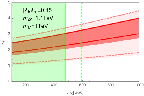
Figure 5: Required values for $\lambda_{L}^{\mu}$ (denoted as $\lambda_{\mu}$ in this figure) and $m_{X}$ to explain the observed values of $R_{K}$ and $R_{K^{\ast}}$ in the model of [13]. This figure has been obtained with fixed $|\lambda_{Q}^{b}\lambda_{Q}^{s}|=0.15$, $m_{L}=1$ TeV and $m_{Q}=1.1$ TeV. The light (dark) red region corresponds to the $R_{K}$ measurement at $1\sigma$ ($2\sigma$), whereas the red lines indicate the same regions for $R_{K^{\ast}}$. The green region is excluded due to $B_{s}-\overline{B_{s}}$ mixing for $m_{Q}=1.1$ TeV. The excluded region would extend up to the dashed green line for $m_{Q}=1$ TeV. Figure taken from [13].

Finally, let us discuss the Dark Matter phenomenology of the model. As explained above, the global $U(1)_{X}$ symmetry is assumed to be conserved, and this implies that a stable state must exist. Assuming that the lighest state charged under $U(1)_{X}$ is the neutral scalar $X$, it constitutes the DM candidate in the model. One then needs to determine whether the observed DM relic density can be achieved in the region of parameter space where the $b\to s$ anomalies are solved, without conflict with other experimental constraints. This is shown in Fig. 6, where contours of $C_{9}^{\mu,\text{NP}}$ are shown in the $m_{L}-m_{X}$ plane. This figure has been obtained with fixed $\lambda_{Q}^{b}=\lambda_{Q}^{s}=\sqrt{0.15}$ and $m_{Q}=1.1$ TeV. For each parameter point, the value of $\lambda_{L}^{\mu}$ is chosen to reproduce the observed DM relic density, which is calculated using MicrOmegas [68]. Large values of $|\lambda_{L}^{\mu}|$ are obtained in this way. For this reason, the most relevant DM annihilation channels for the determination of the relic density with these parameter values are $XX^{\ast}\leftrightarrow\mu^{+}\mu^{-},\nu\nu$. Even though the experimental constraints, in particular those from direct LHC searches for extra quarks, reduce the allowed parameter space substantially, one finds valid regions with $C_{9}^{\mu,\text{NP}}\sim-0.3$. This value would explain the $b\to s$ anomalies at $2\sigma$, see for instance [48]. Interestingly, the model is testable in future direct DM detection experiments, such as XENON1T, as shown in Fig. 6. In the region of parameter space selected for this Figure, the dominant process leading to DM-nucleon scattering is 1-loop photon exchange, with leptons running in the loop. The loop suppression is compensated by the large $\lambda_{L}^{\mu}$ coupling.

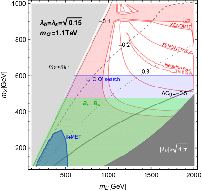
Figure 6: Contours of constant $C_{9}^{\mu,\text{NP}}$ in the $m_{L}-m_{X}$ plane for the model of [13]. This figure has been obtained with fixed $\lambda_{Q}^{b}=\lambda_{Q}^{s}=\sqrt{0.15}$ and $m_{Q}=1.1$ TeV, choosing $\lambda_{L}^{\mu}$ in order to reproduce the observed DM relic density. The colored regions are excluded by various constraints: heavy quark and lepton searches at the LHC (blue), $B_{s}-\overline{B_{s}}$ mixing (green) and direct DM detection experiments (red). The grey regions are excluded due to perturbativity constraints (dark grey region) or by demanding that $X$ is the lightest $U(1)_{X}$-charged state (light grey region). Future direct DM detection prospects are also shown in this plot. Figure taken from [13].

The new states in this model can be discovered at the LHC. For instance, the heavy VL charged lepton can be produced in Drell-Yan processes. Due to the required large values for the $\lambda_{L}^{\mu}$ coupling, this exotic state is expected to decay mainly to a DM particle $X$ (invisible at the LHC) and a muon. Since $U(1)_{X}$ conservation requires the $X$ particles to be produced in pairs, the expected signature is the observation of two energetic muons and large missing energy. Similar events replacing the muons by jets (mainly $b$ jets) are expected for the VL quarks. We conclude the discussion of this model by referring for more details to the original work in [13].

7 Summary and discussion

In this mini-review we have discussed New Physics models that address the $b\to s$ anomalies and link them to the dark matter of the Universe. The interplay between these two areas of particle physics may offer novel model building directions as well as additional phenomenological tests for the proposed scenarios. We have shown that most of the proposed models can be classified into two categories: (i) models in which the $b\to s$ anomalies and the DM production mechanism share a common mediator (such as a heavy $Z^{\prime}$ boson), and (ii) models that induce the NP contributions to explain the $b\to s$ anomalies via loops including the DM particle. These generic ideas have been illustrated with two particular realizations (the models introduced in [2] and [13]), which clearly show that the combination of flavor physics and dark matter leads to new scenarios with a rich phenomenology.

The introduction of a dark sector in a model for the $b\to s$ anomalies can also have phenomenological consequences besides the existence of a DM candidate. For instance, both problems, the dark matter of the Universe and the $b\to s$ anomalies, might be connected to another long-standing question in particle physics: the muon anomalous magnetic moment [4, 73, 74, 75]. Furthermore, it is interesting to note that the introduction of dark matter in some models can help alleaviating some of the most stringent constraints. Indeed, the LHC bounds on some mediators become weaker if they have invisible decay channels [76]. We believe that this is a promising line of research to be pursued in order to fully assess the validity of some scenarios that are currently under experimental tension.

We are living an exciting moment in flavor physics, with several interesting anomalies in B-meson decays. Whether real or not, only time can tell. New LHCb analyses based on larger datasets are expected to appear in the near future, possibly shedding new light on these anomalies. In the longer term, fundamental contributions from the Belle II experiment will also be crucial to settle the issue [77]. In the meantime, an intense model building effort is opening new avenues with rich phenomenological scenarios. The possible connection to one of the central problems in current physics, the nature of the dark matter of the Universe, would definitely be a fascinating outcome of this endeavour.

References

- [1] Planck Collaboration, P. A. R. Ade et al., “Planck 2015 results. XIII. Cosmological parameters,” Astron. Astrophys. 594 (2016) A13, arXiv:1502.01589 [astro-ph.CO].
- [2] D. Aristizabal Sierra, F. Staub, and A. Vicente, “Shedding light on the anomalies with a dark sector,” Phys. Rev. D92 no. 1, (2015) 015001, arXiv:1503.06077 [hep-ph].
- [3] G. Bélanger, C. Delaunay, and S. Westhoff, “A Dark Matter Relic From Muon Anomalies,” Phys. Rev. D92 (2015) 055021, arXiv:1507.06660 [hep-ph].
- [4] B. Allanach, F. S. Queiroz, A. Strumia, and S. Sun, “ models for the LHCb and muon anomalies,” Phys. Rev. D93 no. 5, (2016) 055045, arXiv:1511.07447 [hep-ph]. [Erratum: Phys. Rev.D95,no.11,119902(2017)].
- [5] M. Bauer and M. Neubert, “Flavor anomalies, the 750 GeV diphoton excess, and a dark matter candidate,” Phys. Rev. D93 no. 11, (2016) 115030, arXiv:1512.06828 [hep-ph].
- [6] A. Celis, W.-Z. Feng, and M. Vollmann, “Dirac dark matter and with gauge symmetry,” Phys. Rev. D95 no. 3, (2017) 035018, arXiv:1608.03894 [hep-ph].
- [7] W. Altmannshofer, S. Gori, S. Profumo, and F. S. Queiroz, “Explaining dark matter and B decay anomalies with an model,” JHEP 12 (2016) 106, arXiv:1609.04026 [hep-ph].
- [8] P. Ko, T. Nomura, and H. Okada, “A flavor dependent gauge symmetry, Predictive radiative seesaw and LHCb anomalies,” Phys. Lett. B772 (2017) 547–552, arXiv:1701.05788 [hep-ph].
- [9] P. Ko, T. Nomura, and H. Okada, “Explaining anomaly by radiatively induced coupling in gauge symmetry,” Phys. Rev. D95 no. 11, (2017) 111701, arXiv:1702.02699 [hep-ph].
- [10] J. M. Cline, J. M. Cornell, D. London, and R. Watanabe, “Hidden sector explanation of -decay and cosmic ray anomalies,” Phys. Rev. D95 no. 9, (2017) 095015, arXiv:1702.00395 [hep-ph].
- [11] F. Sala and D. M. Straub, “A New Light Particle in B Decays?,” Phys. Lett. B774 (2017) 205–209, arXiv:1704.06188 [hep-ph].
- [12] J. Ellis, M. Fairbairn, and P. Tunney, “Anomaly-Free Models for Flavour Anomalies,” arXiv:1705.03447 [hep-ph].
- [13] J. Kawamura, S. Okawa, and Y. Omura, “Interplay between the b anomalies and dark matter physics,” Phys. Rev. D96 no. 7, (2017) 075041, arXiv:1706.04344 [hep-ph].
- [14] S. Baek, “Dark matter contribution to anomaly in local model,” arXiv:1707.04573 [hep-ph].
- [15] J. M. Cline, “ decay anomalies and dark matter from vectorlike confinement,” Phys. Rev. D97 no. 1, (2018) 015013, arXiv:1710.02140 [hep-ph].
- [16] J. M. Cline and J. M. Cornell, “ from dark matter exchange,” arXiv:1711.10770 [hep-ph].
- [17] L. Dhargyal, “A simple model to explain the observed muon sector anomalies, small neutrino masses, baryon-genesis and dark-matter,” arXiv:1711.09772 [hep-ph].
- [18] C.-W. Chiang and H. Okada, “A simple model for explaining muon-related anomalies and dark matter,” arXiv:1711.07365 [hep-ph].
- [19] A. Falkowski, S. F. King, E. Perdomo, and M. Pierre, “Flavourful portal for vector-like neutrino Dark Matter and ,” arXiv:1803.04430 [hep-ph].
- [20] G. Arcadi, T. Hugle, and F. S. Queiroz, “The Dark Rises via Kinetic Mixing,” arXiv:1803.05723 [hep-ph].
- [21] S. Jäger and J. Martin Camalich, “On at small dilepton invariant mass, power corrections, and new physics,” JHEP 05 (2013) 043, arXiv:1212.2263 [hep-ph].
- [22] S. Descotes-Genon, L. Hofer, J. Matias, and J. Virto, “On the impact of power corrections in the prediction of observables,” JHEP 12 (2014) 125, arXiv:1407.8526 [hep-ph].
- [23] A. Khodjamirian, T. Mannel, A. A. Pivovarov, and Y. M. Wang, “Charm-loop effect in and ,” JHEP 09 (2010) 089, arXiv:1006.4945 [hep-ph].
- [24] M. Ciuchini, M. Fedele, E. Franco, S. Mishima, A. Paul, L. Silvestrini, and M. Valli, “ decays at large recoil in the Standard Model: a theoretical reappraisal,” JHEP 06 (2016) 116, arXiv:1512.07157 [hep-ph].
- [25] B. Capdevila, S. Descotes-Genon, L. Hofer, and J. Matias, “Hadronic uncertainties in : a state-of-the-art analysis,” JHEP 04 (2017) 016, arXiv:1701.08672 [hep-ph].
- [26] V. G. Chobanova, T. Hurth, F. Mahmoudi, D. Martinez Santos, and S. Neshatpour, “Large hadronic power corrections or new physics in the rare decay ?,” JHEP 07 (2017) 025, arXiv:1702.02234 [hep-ph].
- [27] C. Bobeth, M. Chrzaszcz, D. van Dyk, and J. Virto, “Long-distance effects in from Analyticity,” arXiv:1707.07305 [hep-ph].
- [28] T. Blake, U. Egede, P. Owen, G. Pomery, and K. A. Petridis, “An empirical model of the long-distance contributions to transitions,” arXiv:1709.03921 [hep-ph].
- [29] S. Descotes-Genon, T. Hurth, J. Matias, and J. Virto, “Optimizing the basis of observables in the full kinematic range,” JHEP 05 (2013) 137, arXiv:1303.5794 [hep-ph].
- [30] LHCb Collaboration, R. Aaij et al., “Measurement of Form-Factor-Independent Observables in the Decay ,” Phys. Rev. Lett. 111 (2013) 191801, arXiv:1308.1707 [hep-ex].
- [31] LHCb Collaboration, R. Aaij et al., “Differential branching fraction and angular analysis of the decay ,” JHEP 07 (2013) 084, arXiv:1305.2168 [hep-ex].
- [32] LHCb Collaboration, R. Aaij et al., “Angular analysis of the decay using 3 fb-1 of integrated luminosity,” JHEP 02 (2016) 104, arXiv:1512.04442 [hep-ex].
- [33] LHCb Collaboration, R. Aaij et al., “Angular analysis and differential branching fraction of the decay ,” JHEP 09 (2015) 179, arXiv:1506.08777 [hep-ex].
- [34] Belle Collaboration, A. Abdesselam et al., “Angular analysis of ,” in Proceedings, LHCSki 2016 - A First Discussion of 13 TeV Results: Obergurgl, Austria, April 10-15, 2016. 2016. arXiv:1604.04042 [hep-ex].
- [35] Belle Collaboration, S. Wehle et al., “Lepton-Flavor-Dependent Angular Analysis of ,” Phys. Rev. Lett. 118 no. 11, (2017) 111801, arXiv:1612.05014 [hep-ex].
- [36] ATLAS Collaboration, “Angular analysis of decays in collisions at TeV with the ATLAS detector,” ATLAS-CONF-2017-023 (2017) .
- [37] CMS Collaboration, “Measurement of the and angular parameters of the decay in proton-proton collisions at ,” CMS-PAS-BPH-15-008 (2017) .
- [38] G. Hiller and F. Kruger, “More model-independent analysis of processes,” Phys. Rev. D69 (2004) 074020, arXiv:hep-ph/0310219 [hep-ph].
- [39] LHCb Collaboration, R. Aaij et al., “Test of lepton universality using decays,” Phys. Rev. Lett. 113 (2014) 151601, arXiv:1406.6482 [hep-ex].
- [40] LHCb Collaboration, R. Aaij et al., “Test of lepton universality with decays,” JHEP 08 (2017) 055, arXiv:1705.05802 [hep-ex].
- [41] S. Descotes-Genon, L. Hofer, J. Matias, and J. Virto, “Global analysis of anomalies,” JHEP 06 (2016) 092, arXiv:1510.04239 [hep-ph].
- [42] M. Bordone, G. Isidori, and A. Pattori, “On the Standard Model predictions for and ,” Eur. Phys. J. C76 no. 8, (2016) 440, arXiv:1605.07633 [hep-ph].
- [43] B. Capdevila, S. Descotes-Genon, J. Matias, and J. Virto, “Assessing lepton-flavour non-universality from angular analyses,” JHEP 10 (2016) 075, arXiv:1605.03156 [hep-ph].
- [44] “Heavy flavor averaging group.” http://www.slac.stanford.edu/xorg/hfag/semi/fpcp17/RDRDs.html.
- [45] LHCb Collaboration, R. Aaij et al., “Measurement of the ratio of branching fractions /,” arXiv:1711.05623 [hep-ex].
- [46] D. Buttazzo, A. Greljo, G. Isidori, and D. Marzocca, “B-physics anomalies: a guide to combined explanations,” JHEP 11 (2017) 044, arXiv:1706.07808 [hep-ph].
- [47] B. Capdevila, A. Crivellin, S. Descotes-Genon, J. Matias, and J. Virto, “Patterns of New Physics in transitions in the light of recent data,” JHEP 01 (2018) 093, arXiv:1704.05340 [hep-ph].
- [48] W. Altmannshofer, P. Stangl, and D. M. Straub, “Interpreting Hints for Lepton Flavor Universality Violation,” Phys. Rev. D96 no. 5, (2017) 055008, arXiv:1704.05435 [hep-ph].
- [49] G. D’Amico, M. Nardecchia, P. Panci, F. Sannino, A. Strumia, R. Torre, and A. Urbano, “Flavour anomalies after the measurement,” JHEP 09 (2017) 010, arXiv:1704.05438 [hep-ph].
- [50] G. Hiller and I. Nisandzic, “ and beyond the standard model,” Phys. Rev. D96 no. 3, (2017) 035003, arXiv:1704.05444 [hep-ph].
- [51] L.-S. Geng, B. Grinstein, S. Jäger, J. Martin Camalich, X.-L. Ren, and R.-X. Shi, “Towards the discovery of new physics with lepton-universality ratios of decays,” Phys. Rev. D96 no. 9, (2017) 093006, arXiv:1704.05446 [hep-ph].
- [52] M. Ciuchini, A. M. Coutinho, M. Fedele, E. Franco, A. Paul, L. Silvestrini, and M. Valli, “On Flavourful Easter eggs for New Physics hunger and Lepton Flavour Universality violation,” Eur. Phys. J. C77 no. 10, (2017) 688, arXiv:1704.05447 [hep-ph].
- [53] A. K. Alok, B. Bhattacharya, A. Datta, D. Kumar, J. Kumar, and D. London, “New Physics in after the Measurement of ,” Phys. Rev. D96 no. 9, (2017) 095009, arXiv:1704.07397 [hep-ph].
- [54] T. Hurth, F. Mahmoudi, D. Martinez Santos, and S. Neshatpour, “Lepton nonuniversality in exclusive decays,” Phys. Rev. D96 no. 9, (2017) 095034, arXiv:1705.06274 [hep-ph].
- [55] A. Celis, J. Fuentes-Martin, A. Vicente, and J. Virto, “Gauge-invariant implications of the LHCb measurements on lepton-flavor nonuniversality,” Phys. Rev. D96 no. 3, (2017) 035026, arXiv:1704.05672 [hep-ph].
- [56] W. Altmannshofer, S. Gori, M. Pospelov, and I. Yavin, “Quark flavor transitions in models,” Phys. Rev. D89 (2014) 095033, arXiv:1403.1269 [hep-ph].
- [57] AMS Collaboration, M. Aguilar et al., “Antiproton Flux, Antiproton-to-Proton Flux Ratio, and Properties of Elementary Particle Fluxes in Primary Cosmic Rays Measured with the Alpha Magnetic Spectrometer on the International Space Station,” Phys. Rev. Lett. 117 no. 9, (2016) 091103.
- [58] B. Gripaios, M. Nardecchia, and S. A. Renner, “Linear flavour violation and anomalies in B physics,” JHEP 06 (2016) 083, arXiv:1509.05020 [hep-ph].
- [59] P. Arnan, L. Hofer, F. Mescia, and A. Crivellin, “Loop effects of heavy new scalars and fermions in ,” JHEP 04 (2017) 043, arXiv:1608.07832 [hep-ph].
- [60] E. Ma, “Verifiable radiative seesaw mechanism of neutrino mass and dark matter,” Phys. Rev. D73 (2006) 077301, arXiv:hep-ph/0601225 [hep-ph].
- [61] P. Rocha-Moran and A. Vicente, “Lepton Flavor Violation in a model for the anomalies,” arXiv:1810.02135 [hep-ph].
- [62] A. J. Buras, F. De Fazio, and J. Girrbach, “The Anatomy of Z’ and Z with Flavour Changing Neutral Currents in the Flavour Precision Era,” JHEP 02 (2013) 116, arXiv:1211.1896 [hep-ph].
- [63] W. Altmannshofer and D. M. Straub, “New physics in transitions after LHC run 1,” Eur. Phys. J. C75 no. 8, (2015) 382, arXiv:1411.3161 [hep-ph].
- [64] L. M. Krauss and F. Wilczek, “Discrete Gauge Symmetry in Continuum Theories,” Phys. Rev. Lett. 62 (1989) 1221.
- [65] B. Petersen, M. Ratz, and R. Schieren, “Patterns of remnant discrete symmetries,” JHEP 08 (2009) 111, arXiv:0907.4049 [hep-ph].
- [66] D. Aristizabal Sierra, M. Dhen, C. S. Fong, and A. Vicente, “Dynamical flavor origin of symmetries,” Phys. Rev. D91 no. 9, (2015) 096004, arXiv:1412.5600 [hep-ph].
- [67] W. Porod, F. Staub, and A. Vicente, “A Flavor Kit for BSM models,” Eur. Phys. J. C74 no. 8, (2014) 2992, arXiv:1405.1434 [hep-ph].
- [68] G. Belanger, F. Boudjema, A. Pukhov, and A. Semenov, “micrOMEGAs_3: A program for calculating dark matter observables,” Comput. Phys. Commun. 185 (2014) 960–985, arXiv:1305.0237 [hep-ph].
- [69] A. Greljo, G. Isidori, and D. Marzocca, “On the breaking of Lepton Flavor Universality in B decays,” JHEP 07 (2015) 142, arXiv:1506.01705 [hep-ph].
- [70] A. Alves, S. Profumo, and F. S. Queiroz, “The dark portal: direct, indirect and collider searches,” JHEP 04 (2014) 063, arXiv:1312.5281 [hep-ph].
- [71] A. Alves, A. Berlin, S. Profumo, and F. S. Queiroz, “Dark Matter Complementarity and the Z′ Portal,” Phys. Rev. D92 no. 8, (2015) 083004, arXiv:1501.03490 [hep-ph].
- [72] L. Di Luzio, M. Kirk, and A. Lenz, “One constraint to kill them all?,” arXiv:1712.06572 [hep-ph].
- [73] G. Bélanger and C. Delaunay, “A Dark Sector for , and a Diphoton Resonance,” Phys. Rev. D94 no. 7, (2016) 075019, arXiv:1603.03333 [hep-ph].
- [74] S. Di Chiara, A. Fowlie, S. Fraser, C. Marzo, L. Marzola, M. Raidal, and C. Spethmann, “Minimal flavor-changing models and muon after the measurement,” Nucl. Phys. B923 (2017) 245–257, arXiv:1704.06200 [hep-ph].
- [75] K. Kowalska and E. M. Sessolo, “Expectations for the muon g-2 in simplified models with dark matter,” JHEP 09 (2017) 112, arXiv:1707.00753 [hep-ph].
- [76] D. A. Faroughy, A. Greljo, and J. F. Kamenik, “Confronting lepton flavor universality violation in B decays with high- tau lepton searches at LHC,” Phys. Lett. B764 (2017) 126–134, arXiv:1609.07138 [hep-ph].
- [77] J. Albrecht, F. Bernlochner, M. Kenzie, S. Reichert, D. Straub, and A. Tully, “Future prospects for exploring present day anomalies in flavour physics measurements with Belle II and LHCb,” arXiv:1709.10308 [hep-ph].