On the Dimensional-like Characteristics Arising From Linear Inhomogeneous Approximations

Abstract.

As it follows from the theory of almost periodic functions the set of integer solutions $q$ to the Kronecker system $|\omega_{j}q-\theta_{j}|<\varepsilon\pmod{1}$, $j=1,\ldots,m$, where $1,\omega_{1},\ldots,\omega_{m}$ are linearly independent over $\mathbb{Q}$, is relatively dense in $\mathbb{R}$. The latter means that there exists $L(\varepsilon)>0$ such that any segment of the length $L(\varepsilon)$ contains at least one integer solution to the Kronecker system. We give lower and upper estimate for $L(\varepsilon)$ and show that $L(\varepsilon)=\left(\frac{1}{\varepsilon}\right)^{m+o(1)}$ as $\varepsilon\to 0$ for many cases, including algebraic numbers as well as badly approximable numbers. We use methods of dimension theory and Diophantine approximations of $m$-tuples satisfying Diophantine condition.

1. Introduction

The Kronecker theorem states that if $1,\omega_{1},\ldots,\omega_{m}$ are linearly independent over rationals then for every $\varepsilon>0$ and $\theta_{1},\ldots,\theta_{m}\in\mathbb{R}$ the Kronecker system $|\omega_{j}q-\theta_{j}|<\varepsilon\pmod{1}$, $j=1,\ldots,m$ has an integer solution $q$. One may ask what is an upper or lower bound for such $q$ (more precisely, for the absolute value of the first integer solution $q$ closest to zero) in terms of $\varepsilon,m$ and some properties of $\omega_{1},\ldots,\omega_{m}$? There are papers where the so called effective upper bounds for $|q|$ are given (see [6, 16] and links therein). Usually, such bounds are given under the consideration of algebraic numbers $\omega_{1},\ldots,\omega_{m}$ and, therefore, powerful methods of algebraic number theory (see, for example, [5, 10, 15]) are used. A typical bound is $|q|\leq C\left(\frac{1}{\varepsilon}\right)^{d-1}$, where $d=\left[\mathbb{Q}(\omega_{1},\ldots,\omega_{m})\colon\mathbb{Q}\right]$ and the constant $C$ depends on $m$, $d$ and the heights and degrees of $\omega_{1},\ldots,\omega_{m}$. The effectiveness of a bound means that the constant $C$ can be directly calculated. It is well-known that if one removes the requirement of effectiveness, the exponent $d-1$ may be changed to (the stronger one) $m+\delta$ for any $\delta>0$ (see, for example, remark 3.1 in [6] or Theorem 2.1 in [12]).

On the other hand, as the theory of almost periodic functions (see [14]) says, the set of integer solutions to the Kronecker system are relatively dense, namely, there is $L(\varepsilon)>0$ such that every segment of length $L(\varepsilon)$ contains an integer solution. Now one may ask: what are possible lower or upper bounds for $L(\varepsilon)$ or what is the growth rate of $L(\varepsilon)$ as $\varepsilon$ tends to zero? Here we use a dimension theory approach (see [3, 11, 13]) combined with Diophantine approximations (see [8, 9, 15]) to provide some lower and upper bounds for $L(\varepsilon)$. Despite that these bounds are ineffective, we get additional information (for example, about the distribution of such solutions and exact values of dimensional-like characteristics) and treat a more general than just an algebraic set of $\omega$’s, providing a different view on the problem. This complements some known results, namely, effective versions (obtained via algebraic number theory [6, 16]) and quantitative versions (derived from transference principles [4]) of the Kronecker theorem. To state our results precisely, we need some concepts.

Diophantine dimension

A subset $\mathcal{R}\subset\mathbb{R}^{n}$ is called relatively dense in $\mathbb{R}^{n}$ if there is a real number $L>0$ such that the set $(a+[0,L]^{n})\cap\mathcal{R}$ is not empty for all $a\in\mathbb{R}^{n}$.

Let $\mathfrak{R}=\{\mathcal{R}_{\varepsilon}\}$, $\varepsilon>0$, be a family of relatively dense in $\mathbb{R}^{n}$ subsets $\mathcal{R}_{\varepsilon}\subset\mathbb{R}^{n}$ such that $\mathcal{R}_{\varepsilon_{1}}\supset\mathcal{R}_{\varepsilon_{2}}$ provided by $\varepsilon_{1}>\varepsilon_{2}$. Let $L(\varepsilon)>0$ be a real number such that $(a+[0,L(\varepsilon)]^{n})\cap\mathcal{R}_{\varepsilon}$ is not empty for all $a\in\mathbb{R}^{n}$. Let $l_{\mathfrak{R}}(\varepsilon)$ be the infimum of all such $L(\varepsilon)$. Then $l_{\mathfrak{R}}(\varepsilon)$ is the inclusion length for $\mathcal{R}_{\varepsilon}$. The value

(1.1) $$\mathfrak{Di}(\mathfrak{R}):=\limsup\limits_{\varepsilon\to 0+}\frac{\ln l_{\mathfrak{R}}(\varepsilon)}{\ln\left(1/\varepsilon\right)}$$

is called the Diophantine dimension of $\mathfrak{R}$. Also we consider the lower Diophantine dimension of $\mathfrak{R}$ defined as

(1.2) $$\mathfrak{di}(\mathfrak{R}):=\liminf\limits_{\varepsilon\to 0+}\frac{\ln l_{\mathfrak{R}}(\varepsilon)}{\ln\left(1/\varepsilon\right)}.$$

Box-counting dimension

Let $\mathcal{X}$ be a compact metric space and let $N_{\varepsilon}(\mathcal{X})$ denote the minimal number of open balls of radius $\varepsilon$ required to cover $\mathcal{X}$. The values

(1.3) $$\begin{split}\underline{\dim}_{B}\mathcal{X}&=\liminf_{\varepsilon\to 0+}\frac{\ln N_{\varepsilon}(\mathcal{X})}{\ln(1/\varepsilon)},\\ \overline{\dim}_{B}\mathcal{X}&=\limsup_{\varepsilon\to 0+}\frac{\ln N_{\varepsilon}(\mathcal{X})}{\ln(1/\varepsilon)}\end{split}$$

are called lower box dimension and upper box dimension respectively.

Diophantine condition

For $\theta\in\mathbb{R}^{m}$ we denote by $|\theta|_{m}$ the distance from $\theta$ to $\mathbb{Z}^{m}$. Clearly, $|\cdot|$ defines a metric on $m$-dimensional flat torus $\mathbb{T}^{m}=\mathbb{R}^{m}/\mathbb{Z}^{m}$.

We say that an $m$-tuple $\omega=(\omega_{1},\ldots,\omega_{m})$ of real numbers satisfy the Diophantine condition of order $\nu\geq 0$ if for some $C_{d}>0$ and all natural $q$ the inequality

(1.4) $$|\omega q|_{m}\geq C_{d}\left(\frac{1}{q}\right)^{\frac{1+\nu}{m}}$$

holds.

For a function $\phi\colon\mathbb{R}^{n}\to\mathcal{X}$ let $\mathcal{O}(\phi)$ be the closure of $\bigcup\limits_{\boldsymbol{t}\in\mathbb{R}^{n}}\phi(\boldsymbol{t})$ in $\mathcal{X}$ and let $\mathring{\mathcal{O}}(\phi)$ be the closure of $\bigcup\limits_{\boldsymbol{q}\in\mathbb{Z}^{n}}\phi(\boldsymbol{q})$ in $\mathcal{X}$.

Theorem 1.1.

Let $A$ be an $(m\times n)$-matrix with real coefficients and $\theta\in\mathring{\mathcal{O}}(\phi)$, where $\phi\colon\mathbb{R}^{n}\to\mathbb{T}^{m}$ is defined by $\phi(\boldsymbol{t}):=A\boldsymbol{t}$; then the set $\mathcal{R}_{\varepsilon}$ of integer solutions $\boldsymbol{q}\in\mathbb{Z}^{n}$ to

(1.5) $$|A\boldsymbol{q}-\theta|_{m}<\varepsilon$$

is relatively dense in $\mathbb{R}^{n}$ and the lower Diophantine dimension of $\mathfrak{R}=\{\mathcal{R}_{\varepsilon}\}$ satisfies

(1.6) $$\mathfrak{di}(\mathfrak{R})\geq\frac{d-n}{n},$$

where $d=\underline{\dim}_{B}\mathcal{O}(\hat{\phi})$ and $\hat{\phi}\colon\mathbb{R}^{n}\to\mathbb{T}^{m+n}$ is defined by $\hat{\phi}(\boldsymbol{t}):=\hat{A}\boldsymbol{t}$, $\hat{A}=\begin{bmatrix}E\\ A\end{bmatrix}.$

The proof of theorem 1.1 is given at the end of section 3.

Theorem 1.2.

Suppose that $1,\omega_{1},\ldots,\omega_{m}$ are linearly independent over $\mathbb{Q}$ and let $\omega=(\omega_{1},\ldots,\omega_{m})$ satisfy the Diophantine condition of order $\nu\geq 0$ such that $\nu(m-1)<1$; then for all $\theta_{1},\ldots,\theta_{m}\in\mathbb{R}$ and $\varepsilon>0$ the set $\mathcal{K}_{\varepsilon}$ of integer solutions $q$ to

(1.7) $$|\omega q-\theta|_{m}<\varepsilon,$$

is relatively dense in $\mathbb{R}$ and the Diophantine dimension $\mathfrak{Di}(\mathfrak{K})$ of $\mathfrak{K}=\{\mathcal{K}_{\varepsilon}\}$ satisfies the inequality

(1.8) $$\mathfrak{Di}(\mathfrak{K})\leq\frac{(1+\nu)m}{1-\nu(m-1)}.$$

The proof of theorem 1.2 is given at the end of section 4.

Estimates (1.6) and (1.8) can be used to prove the following corollary (the proof is outlined in section 5).

Corollary 1.3.

There is a set of full measure $\Omega_{m}\subset\mathbb{R}^{m}$ such that for any $\omega=(\omega_{1},\ldots,\omega_{m})\in\Omega_{m}$ the Diophantine dimensions of $\mathfrak{K}$ (see the previous theorem) satisfy

(1.9) $$\mathfrak{di}(\mathfrak{K})=\mathfrak{Di}(\mathfrak{K})=m.$$

In particular, badly approximable and algebraic $m$-tuples, which are linearly independent over $\mathbb{Q}$, satisfy the above conditions.

Thus, within the assumptions of corollary 1.3, for all small $\delta>0$ and for some ineffective constants $C^{+}(\delta)$ and $C_{-}(\delta)$, we have an integer solution to (1.7) in each interval of length $C^{+}(\delta)\left(\frac{1}{\varepsilon}\right)^{m+\delta}$ and there are gaps of length $C_{-}(\delta)\left(\frac{1}{\varepsilon}\right)^{m-\delta}$ with no integer solutions.

The main idea of our approach is as follows. To study integer solutions $\boldsymbol{q}\in\mathbb{Z}^{n}$ to (1.5) (the discrete problem) we consider the extended system with the matrix

(1.10) $$\hat{A}=\begin{bmatrix}E\\ A\end{bmatrix}$$

and with respect to $\boldsymbol{t}\in\mathbb{R}^{n}$ (the continuous problem). By the choice of $\hat{A}$, any solution $\boldsymbol{t}$ of the extended system is close to $\mathbb{Z}^{m}$ and, therefore, the corresponding Diophantine dimensions of the discrete problem and the continuous problem coincide (see proposition 2.2). Due to the linearity of $\hat{A}$ (which is essential) the corresponding Diophantine dimension of the family of $\varepsilon$-solutions to the extended system is equal to the Diophantine dimension of the almost periodic function $\hat{\phi}(\boldsymbol{t}):=\hat{A}\boldsymbol{t}$ defined by the family of $\varepsilon$-almost periods of $\hat{\phi}(\cdot)$ (see proposition 2.1). Thus, it is enough to study the Diophantine dimension of $\hat{\phi}$. For the latter purpose we will use developed methods from our earlier works [1, 2].

A research interest in such properties, in addition to the purely algebraic one, may come from almost periodic dynamics (see [1, 2, 7, 13]). For example, it is well-known that some number-theoretical phenomena appear in the linearization of circle diffeomorphisms as well as in KAM theory (see [7, 12]). As it follows from the arithmetical nature of almost periods there is a strong connection between them and the Diophantine approximations of the Fourier exponents. More precisely, the latter affects the growth rate of the inclusion length. To study such a connection, a definition of Diophantine dimension was given (see [1]). A method for upper estimates of the inclusion length (and, therefore, of the Diophantine dimension) firstly appeared in [13] for the case of badly approximable numbers. In [1] it was generalized for quasi-periodic functions with one irrational frequency that satisfies the Diophantine condition. In the present paper we generalize such an approach (theorem 4.3) to give an upper estimate of the Diophantine dimension for quasi-periodic functions with frequency $m$-tuple, satisfying simultaneous Diophantine condition. A dimensional argument (as in theorem 3.1) to provide a lower estimate of the Diophantine dimension firstly appeared in [2], where the recurrence properties of almost periodic dynamics were studied (as well as in [13]).

This paper is organized as follows. In section 2 we begin with some basic definitions from the theory of almost periodic functions. Next, we show how the discrete problem is simply connected with the continuous one. In section 3 we give a lower bound for the Diophantine dimension (theorem 3.1), using a dimensional argument, namely, we use the lower box dimension of the orbit closure. In section 4 we present an upper bound for the case of $m$-tuple, satisfying simultaneously Diophantine condition (theorem 4.3), for what we need a proper sequence of simultaneous denominators (=convergents), provided by theorem 4.2. Section 5 is devoted to the discussion of the presented approach and its consequences, in particular, concerning the Kronecker theorem.

2. Preliminaries

Almost periodic functions

Let $\mathbb{G}$ be a locally compact abelian group and let $\mathcal{X}$ be a complete metric space endowed with a metric $\varrho_{\mathcal{X}}$. A continuous function $\phi\colon\mathbb{G}\to\mathcal{X}$ is called almost periodic if for every $\varepsilon>0$ the set $\mathcal{T}_{\varepsilon}(\phi)$ of $\tau\in\mathbb{G}$ such that

(2.1) $$\varrho\left(\phi(\cdot+\tau),\phi(\cdot)\right)_{\infty}:=\sup_{t\in\mathbb{G}}\varrho_{\mathcal{X}}(\phi(t+\tau),\phi(t))\leq\varepsilon$$

is relatively dense in $\mathbb{G}$, i. e. there is a compact set $\mathcal{K}=\mathcal{K}(\varepsilon)\subset\mathbb{G}$ such that $\left(g+\mathcal{K}\right)\cap\mathcal{T}_{\varepsilon}(\phi)\not=\emptyset$ for all $g\in\mathbb{G}$. Here $\tau\in\mathcal{T}_{\varepsilon}(\phi)$ is called an $\varepsilon$-almost period of $\phi$. The following theorem is due to Bochner (see theorem 1.2 and remark 1.4 in [14]).

Theorem 2.1.

A bounded continuous function $\phi(\cdot)$ is almost periodic if and only if every sequence $\{\phi(\cdot+\tau_{n})\}$, $\tau_{n}\in\mathbb{G},n=1,2,\ldots$, contains a uniformly convergent subsequence.

Example 2.2.

Let $\mathbb{G}=\mathbb{R}^{n}$ and $\mathcal{X}=\mathbb{T}^{m}$, where $\mathbb{T}^{m}:=\mathbb{T}^{m}/\mathbb{Z}^{m}$ is $m$-dimensional flat torus. For $\theta\in\mathbb{T}^{m}$ let $|\theta|_{m}$ be the distance from $\theta$ (more formally, from any representative of $\theta$) to $\mathbb{Z}^{m}$. Then a metric on $\mathbb{T}^{m}$ is given by

(2.2) $$\varrho_{m}(\theta_{1},\theta_{2}):=|\theta_{1}-\theta_{2}|_{m}.$$

Note that the product $\theta t$ for $\theta\in\mathbb{T}^{m}$ and $t\in\mathbb{R}$ is well-defined, as well as any function $f\colon\mathbb{R}^{s}\to\mathbb{R}^{m}$ can be considered as a function $f\colon\mathbb{R}^{s}\to\mathbb{T}^{m}$.

In this case it is quite clear that continuous periodic functions are almost periodic (by definition) and any sum of continuous periodic functions is almost periodic (by the Bochner theorem). Consider $\phi\colon\mathbb{R}^{n}\to\mathbb{T}^{m}$ defined as $\phi(\boldsymbol{t}):=A\boldsymbol{t}$, where $A$ is an $m\times n$ matrix with real coefficients. It is clear that the function $\phi(\cdot)$ is almost periodic due to its additivity and compactness of $\mathbb{T}^{m}$.

A more simple example (also known as a linear flow on $\mathbb{T}^{m}$) appears when $n=1$ and $\phi(t):=(\omega_{1}t,\ldots,\omega_{m}t)$, where $\omega_{1},\ldots,\omega_{m}\in\mathbb{R}$.

Basic constructions

Further (see propositions 2.1 and 2.2) we will have to show some relations between the Diophantine dimensions of two families $\mathfrak{R}^{\prime}=\{\mathcal{R}^{\prime}_{\varepsilon}\}$ and $\mathfrak{R}^{\prime\prime}=\{\mathcal{R}^{\prime\prime}_{\varepsilon}\}$. Note that in order to show the inequality $\mathfrak{Di}(\mathfrak{R}^{\prime})\leq\mathfrak{Di}(\mathfrak{R}^{\prime\prime})$ it is sufficient to show the inclusion $\left(\mathcal{R}^{\prime\prime}_{C\varepsilon}+\boldsymbol{t}_{0}(\varepsilon)\right)\subset\mathcal{R}^{\prime}_{\varepsilon}$ for some constant $C>0$ and $\boldsymbol{t}_{0}(\varepsilon)\in\mathbb{R}^{n}$.

We will deal with the case when $\mathcal{R}_{\varepsilon}$ is a set of integer solutions to the Kronecker system or, more generally, the set of moments of return (integer or real) in $\varepsilon$-neighbourhood of a point in the closure of almost periodic trajectory.

Let $\mathbb{G}=\mathbb{R}^{n}$ and let $\mathcal{X}$ be a complete metric space. Consider a non-constant almost periodic function $\phi\colon\mathbb{R}^{n}\to\mathcal{X}$. By definition, the set $\mathcal{T}_{\varepsilon}(\phi)$ of $\varepsilon$-almost periods of $\phi$ is relatively dense. We use the notations $\mathfrak{Di}(\phi)$ and $\mathfrak{di}(\phi)$ for the Diophantine dimensions of the corresponding family $\{\mathcal{T}_{\varepsilon}(\phi)\}$ and we call them the Diophantine dimension of $\phi$ and the lower Diophantine dimension of $\phi$ respectively. Note that the set $\mathcal{T}_{\varepsilon}(\phi)\cap\mathbb{Z}^{n}$ is relatively dense too. We use the notations $\mathring{\mathfrak{Di}}(\phi)$ and $\mathring{\mathfrak{di}}(\phi)$ for the Diophantine dimension and the lower Diophantine dimension of the corresponding family $\{\mathcal{T}_{\varepsilon}(\phi)\cap\mathbb{Z}^{n}\}$.

Recall, that we use the notations $\mathcal{O}(\phi)$ and $\mathring{\mathcal{O}}(\phi)$ for the closure (in $\mathcal{X}$) of $\phi(\mathbb{R}^{n})$ and $\phi(\mathbb{Z}^{n})$ respectively. The following example shows that these sets can differ.

Example 2.3.

Let $\phi\colon\mathbb{R}^{2}\to\mathbb{T}^{2}$ and $\phi(\boldsymbol{t})=(t_{1},\sqrt{2}t_{2})$. Here $\mathcal{O}(\phi)$ is entire $\mathbb{T}^{2}$ and $\mathring{\mathcal{O}}(\phi)$ is just a segment.

For $\varepsilon>0$ and $x\in\mathcal{O}(\phi)$ consider the system of inequalities with respect to $\boldsymbol{t}\in\mathbb{R}^{n}$:

(2.3) $$\varrho_{\mathcal{X}}(\phi(\boldsymbol{t}),x)\leq\varepsilon.$$

It is easy to see that if $\boldsymbol{t}=\boldsymbol{t}_{0}$ is a solution to (2.3) and $\tau\in\mathcal{T}_{\varepsilon}(\phi)$ then $\boldsymbol{t}_{0}+\tau$ is a $2\varepsilon$-solution (i. e. with $\varepsilon$ changed to $2\varepsilon$) to (2.3). Thus, the set of solutions to (2.3) is relatively dense. We use the notations $\mathfrak{Di}(\phi;x)$ and $\mathfrak{di}(\phi;x)$ for the corresponding Diophantine dimensions. Note that the given argument provides the inequalities $\mathfrak{Di}(\phi;x)\leq\mathfrak{Di}(\phi)$ and $\mathfrak{di}(\phi;x)\leq\mathfrak{di}(\phi)$.

For $\varepsilon>0$ and $x\in\mathring{\mathcal{O}}(\phi)$ consider the system of inequalities with respect to $\boldsymbol{q}\in\mathbb{Z}^{n}$:

(2.4) $$\varrho_{\mathcal{X}}(\phi(\boldsymbol{q}),x)\leq\varepsilon.$$

As in the previous case, one can show that the set of solutions to 2.4 is relatively dense. Here we use the notations $\mathring{\mathfrak{Di}}(\phi;x)$ and $\mathring{\mathfrak{di}}(\phi;x)$ for the corresponding Diophantine dimensions.

Now for $\phi\colon\mathbb{R}^{n}\to\mathbb{T}^{m}$ defined by $\phi(\boldsymbol{t})=A\boldsymbol{t}$ (as in example 2.2) and $\theta\in\mathcal{O}(\phi)$ consider the system

(2.5) $$|A\boldsymbol{t}-\theta|_{m}\leq\varepsilon.$$

Proposition 2.1.

For $\phi(\cdot)$ defined above we have

(2.6) $$\begin{split}\mathfrak{Di}(\phi;\theta)&=\mathfrak{Di}(\phi),\\ \mathfrak{di}(\phi;\theta)&=\mathfrak{di}(\phi).\end{split}$$

Proof.

Let $\boldsymbol{t}_{0}$ be a fixed solution to $\eqref{EQ: TorusLinearSystem}$ and let $\tau$ be an arbitrary solution to $\eqref{EQ: TorusLinearSystem}$. For $\tau^{\prime}=\tau-\boldsymbol{t}_{0}$ we have

(2.7) $$|A(\tau^{\prime}+\boldsymbol{t})-A(\boldsymbol{t})|_{m}=|A\tau-A\boldsymbol{t}_{0}|_{m}\leq|A\tau-\theta|_{m}+|A\boldsymbol{t}_{0}-\theta|_{m}\leq 2\varepsilon.$$

Thus, $\tau^{\prime}\in\mathcal{T}_{2\varepsilon}(\phi)$ and, consequently, $\mathfrak{Di}(\phi;\theta)\geq\mathfrak{Di}(\phi)$ and $\mathfrak{di}(\phi;\theta)\geq\mathfrak{di}(\phi)$. The inverse inequalities were shown before. ∎

Additivity of $\phi(\cdot)$ plays a central role in the proof of proposition 2.1. Consider the following

Example 2.4.

Let $\phi\colon\mathbb{R}\to\mathbb{T}^{2}$ be given by $\phi(t):=\left(\sin(2\pi t)\sin(2\pi\sqrt{2}t),\cos(2\pi t)\right)$. It is clear that every integer is a solution to the system $|\phi(\boldsymbol{t})|_{m}<\varepsilon$ (i. e. for $\theta=0$). Thus, $\mathfrak{Di}(\phi;0)=0$, but as it will be shown below $\mathfrak{Di}(\phi)=1$.

Our purpose is to study the set of integer solutions to (2.5), i.e. solutions $\boldsymbol{q}\in\mathbb{Z}^{n}$ for the system (we call it also the Kronecker system)

(2.8) $$|A\boldsymbol{q}-\theta|_{m}\leq\varepsilon,$$

where $\theta\in\mathring{\mathcal{O}}(\phi)\subset\mathbb{T}^{n}$. For a transition to the continuous problem we consider the extended system with respect to $\boldsymbol{t}\in\mathbb{R}^{n}$:

(2.9) $$|\hat{A}\boldsymbol{t}-\hat{\theta}|_{M}\leq\varepsilon,$$

where $M=n+m$, $\hat{\theta}=(0,\ldots,0,\theta_{1},\ldots,\theta_{m})\in\mathbb{T}^{M}$ and $\hat{A}$ is the $(M\times n)$-matrix defined in (1.10). In other words, we are looking for real solutions $\boldsymbol{t}$ of (2.8), satisfying $n$ additional conditions: $|t_{1}|_{1}\leq\varepsilon,\ldots,|t_{n}|_{1}\leq\varepsilon$. It is clear that an integer solution to (2.8) is also a solution to (2.9). As we said the set of solutions to (2.8) is relatively dense. Let $\hat{\phi}(\boldsymbol{t}):=\hat{A}\boldsymbol{t}$ be the corresponding almost periodic function (see example 2.2). We have the following

Proposition 2.2.

For the set of solutions to (2.8) we have

(2.10) $$\begin{split}\mathring{\mathfrak{Di}}(\phi;\theta)&=\mathfrak{Di}(\hat{\phi}),\\ \mathring{\mathfrak{di}}(\phi;\theta)&=\mathfrak{di}(\hat{\phi}).\end{split}$$

Proof.

It is clear that $\hat{\phi}=\hat{A}\boldsymbol{t}$ is Lipschitz continuous, i. e. there is $C>0$ such that $|\hat{A}\boldsymbol{t}^{\prime}-\hat{A}\boldsymbol{t}^{\prime\prime}|_{M}\leq\varepsilon$ provided by $|\boldsymbol{t}^{\prime}-\boldsymbol{t}^{\prime\prime}|\leq C\varepsilon$. Let $\tau$ be a $\frac{C}{2}\varepsilon$-solution to (2.9). It follows that there is $\boldsymbol{q}\in\mathbb{Z}^{n}$ such that $|\boldsymbol{q}-\tau|\leq\frac{C}{2}\varepsilon$ and, consequently, $|\hat{A}\boldsymbol{q}-\hat{A}\boldsymbol{\tau}|_{M}\leq\varepsilon$. Thus,

(2.11) $$|A\boldsymbol{q}-\theta|_{m}\leq|A\tau-\theta|_{m}+|A\tau-A\boldsymbol{q}|_{m}\leq 2\varepsilon.$$

We showed that $\mathring{\mathfrak{Di}}(\phi;\theta)\leq\mathfrak{Di}(\hat{\phi})$ and $\mathring{\mathfrak{di}}(\phi;\theta)\leq\mathfrak{di}(\hat{\phi})$. The inequalities $\mathring{\mathfrak{Di}}(\phi;\theta)\geq\mathfrak{Di}(\hat{\phi})$ and $\mathring{\mathfrak{di}}(\phi;\theta)\geq\mathfrak{di}(\hat{\phi})$ were shown before. ∎

A similar reasoning shows that $\mathfrak{Di}(\hat{\phi})=\mathring{\mathfrak{Di}}(\hat{\phi})$.

So, the set of solutions to the Kronecker system (2.8) is relatively dense and to study its Diophantine dimension, it is sufficient, by Propositions 2.1 and 2.2, to study the Diophantine dimension of the almost periodic function $\hat{\phi}(\cdot)$, corresponding to the extended system (2.9).

3. A lower estimate via dimension theory

Let $\varphi\colon\mathbb{R}^{n}\to\mathcal{X}$ be a non-constant almost periodic function. In particular, $\varphi$ is uniformly continuous. Let $\delta(\varepsilon)$ be such that $\varrho_{\mathcal{X}}(\varphi(\boldsymbol{t}_{1}),\varphi(\boldsymbol{t}_{2}))\leq\varepsilon$ provided by $\|\boldsymbol{t}_{1}-\boldsymbol{t}_{2}\|_{\infty}\leq\delta(\varepsilon)$, where $\|\cdot\|_{\infty}$ is the sup-norm in $\mathbb{R}^{n}$. Let $\delta^{*}(\varepsilon)$ be the supremum of such numbers $\delta(\varepsilon)$. Consider the values

(3.1) $$\begin{split}\overline{\Delta}(\varphi)&:=\limsup\limits_{\varepsilon\to 0+}\frac{\ln\delta^{*}(\varepsilon)}{\ln\varepsilon},\\ \underline{\Delta}(\varphi)&:=\liminf\limits_{\varepsilon\to 0+}\frac{\ln\delta^{*}(\varepsilon)}{\ln\varepsilon}.\end{split}$$

We say that a map $\chi\colon\mathcal{X}\to\mathcal{Y}$, where $\mathcal{X}$ and $\mathcal{Y}$ are complete metric spaces, satisfies a local Hölder condition with an exponent $\alpha\in(0,1]$ if there are constants $C>0$ and $\varepsilon_{0}>0$ such that $\varrho_{\mathcal{Y}}(\chi(x_{1}),\chi(x_{2}))\leq C\varrho_{\mathcal{X}}{(x_{1},x_{2})}^{\alpha}$ provided by $\varrho_{\mathcal{X}}(x_{1},x_{2})<\varepsilon_{0}$.

It is clear that if $\varphi(\cdot)$ satisfies a local Hölder condition with an exponent $\alpha\in(0,1]$ then $\underline{\Delta}(\varphi)\leq\overline{\Delta}(\varphi)\leq\frac{1}{\alpha}$.

Consider the hull $\mathcal{H}(\varphi)$ of an almost periodic function $\varphi\colon\mathbb{R}^{n}\to\mathcal{Y}$, where $\mathcal{Y}$ is a complete metric space, defined as the closure of its translates $\{\varphi(\cdot+\boldsymbol{t})\ |\ \boldsymbol{t}\in\mathbb{R}^{n}\}$ in the uniform norm. By Theorem 2.1, $\mathcal{H}(\varphi)$ is a compact subset in the space of bounded continuous functions with the uniform norm. We will estimate the box dimensions of $\mathcal{H}(\varphi)$ in the following theorem.

Theorem 3.1.

(3.2) $$\begin{split}\frac{1}{n}\overline{\dim}_{B}\mathcal{H}(\varphi)&\leq\mathfrak{Di}(\varphi)+\overline{\Delta}(\varphi),\\ \frac{1}{n}\underline{\dim}_{B}\mathcal{H}(\varphi)&\leq\mathfrak{di}(\varphi)+\underline{\Delta}(\varphi).\end{split}$$

Proof.

Let $\varepsilon>0$. We will show that for all $\varphi(\cdot+\boldsymbol{t})$, $\boldsymbol{t}\in\mathbb{R}^{n}$ there exists $\overline{\boldsymbol{t}}\in[0,l_{\varphi}(\varepsilon)]^{n}$ such that

(3.3) $$\|\varphi(\cdot+\boldsymbol{t})-\varphi(\cdot+\overline{\boldsymbol{t}})\|_{\infty}\leq\varepsilon.$$

Indeed, there is an $\varepsilon$-almost period $\tau\in[-\boldsymbol{t},-\boldsymbol{t}+l_{\varphi}(\varepsilon)]^{n}$ for $\varphi(\cdot)$. Then $\overline{\boldsymbol{t}}:=\boldsymbol{t}+\tau$ is what we wanted. Now for arbitrary $\overline{\varphi}\in\mathcal{H}(\varphi)$ there exists $\boldsymbol{t}\in\mathbb{R}^{n}$ such that $\|\overline{\varphi}(\cdot)-\varphi(\cdot+\boldsymbol{t})\|_{\infty}\leq\varepsilon$ and, consequently,

(3.4) $$\|\overline{\varphi}(\cdot)-\varphi(\cdot+\overline{\boldsymbol{t}})\|_{\infty}\leq 2\varepsilon.$$

For convenience’ sake if $\mathcal{Q}\subset\mathbb{R}^{n}$ let $\mathcal{Q}_{\varphi}:=\{\varphi(\cdot+\boldsymbol{t})\ |\ \boldsymbol{t}\in\mathcal{Q}\}\subset\mathcal{H}(\varphi)$. It follows from (3.4) that it is sufficient to cover the set $[0,l_{\varphi}(\varepsilon)]^{n}_{\varphi}$ by open balls. Let $\mathcal{B}_{\varepsilon}(\varphi(\cdot+\boldsymbol{t}))$ be the open ball centered at $\varphi(\cdot+\boldsymbol{t})$ with radius $\varepsilon$. It is clear that for $\boldsymbol{t}=(t_{1},\ldots,t_{n})$

(3.5) $$\mathcal{B}_{\varepsilon}(\varphi(\cdot+\boldsymbol{t}))\supset\left(\prod\limits_{j=1}^{n}\left[t_{j}-\frac{\delta^{*}(\varepsilon)}{2},t_{j}+\frac{\delta^{*}(\varepsilon)}{2}\right]\right)_{\varphi}.$$

Thus, the set $[0,l_{\varphi}(\varepsilon)]^{n}_{\varphi}$ can be covered by $\left(\frac{l_{\varphi}(\varepsilon)}{\delta^{*}(\varepsilon)}+1\right)^{n}$ open balls of radius $\varepsilon$ and, consequently, the set $\mathcal{H}(\varphi)$ can be covered by the same number of balls of radius $3\varepsilon$. Therefore, $N_{3\varepsilon}(\mathcal{H}(\varphi))\leq\left(\frac{l_{\varphi}(\varepsilon)}{\delta^{*}(\varepsilon)}+1\right)^{n}$ and

(3.6) $$\frac{\ln N_{3\varepsilon}(\mathcal{H}(\varphi))}{\ln(1/\varepsilon)}\leq n\frac{\ln\left(\frac{l_{\varphi}(\varepsilon)}{\delta^{*}(\varepsilon)}+1\right)}{\ln(1/\varepsilon)}.$$

Taking it to the lower/upper limit in (3.6) we finish the proof. ∎

It is easy to show that if $\chi(\cdot)$ satisfies a local Hölder condition with an exponent $\alpha\in(0,1]$ then $\overline{\dim}_{B}(\chi(\mathcal{X}))\leq\frac{\overline{\dim}_{B}\mathcal{X}}{\alpha}$ and $\underline{\dim}_{B}(\chi(\mathcal{X}))\leq\frac{\underline{\dim}_{B}\mathcal{X}}{\alpha}$.

Consider $\pi_{\mathcal{X}}\colon\mathcal{H}(\varphi)\to\mathcal{X}$ defined by $\pi_{\mathcal{X}}(\overline{\varphi}):=\overline{\varphi}(0)$ for $\overline{\varphi}\in\mathcal{H}(\varphi)$. It is clear that $\pi_{\mathcal{X}}$ is a Lipschitz map. From Theorem 2.1 it follows that $\pi_{\mathcal{X}}(\mathcal{H}(\varphi))=\mathcal{O}(\varphi)$. Thus, $\underline{\dim}_{B}\mathcal{O}(\varphi)\leq\underline{\dim}_{B}\mathcal{H}(\varphi)$. Now we can prove theorem 1.1.

Proof of theorem 1.1.

Using proposition 2.2 we transit to continuous problem (1.5). Proposition 2.1 with Theorem 3.1 applied to $\varphi(\boldsymbol{t}):=\hat{A}\boldsymbol{t}$ give the desired result: it is quite clear that $\varphi$ is Lipschitz continuous and, consequently, $\underline{\Delta}(\varphi)\leq 1$. Now we use $\underline{\dim}_{B}\mathcal{O}(\varphi)\leq\underline{\dim}_{B}\mathcal{H}(\varphi)$ and the second inequality in (3.2). ∎

4. An upper estimate via Diophantine approximations

One of the basic properties of the Diophantine dimension is given by the following simple lemma (see [1]).

Lemma 4.1.

Let $\varphi\colon\mathbb{R}^{n}\to\mathcal{X}$ be almost periodic and let $\chi\colon\mathcal{X}\to\mathcal{Y}$ satisfy a local Hölder condition with an exponent $\alpha\in(0,1]$; then

(4.1) $$\begin{split}\mathfrak{Di}(\chi\circ\varphi)&\leq\frac{\mathfrak{Di}(\varphi)}{\alpha},\\ \mathfrak{di}(\chi\circ\varphi)&\leq\frac{\mathfrak{di}(\varphi)}{\alpha}.\end{split}$$

Remark 4.1.

Let the function $\Phi\colon\mathbb{T}^{m+1}\to\mathcal{X}$, where $\mathcal{X}$ is a complete metric space, satisfy a local Hölder condition with an exponent $\alpha\in(0,1]$ and let $\omega_{1},\ldots,\omega_{m}$ be real numbers. The function $\varphi(t):=\Phi(t,\omega_{1}t,\ldots,\omega_{m}t)$, $t\in\mathbb{R}$, is almost periodic as the image of an almost periodic function under a uniformly continuous map. By Lemma 4.1, $\mathfrak{Di}(\varphi)\leq\frac{\mathfrak{Di}(v)}{\alpha}$, where $v(t):=(t,\omega_{1},\ldots,\omega_{m}t)$ is a linear flow on $\mathbb{T}^{m+1}$. So it is sufficient to estimate $\mathfrak{Di}(v)$.

Since there are no algorithms (similar to the classical continued fraction expansion), which could provide a sequence of convergents $\{q_{k}\}$ with ¡¡good¿¿ properties, for the simultaneous approximation case, we prove the existence of convergents with required properties. At first we need the classical Dirichlet theorem.

Theorem 4.2.

Let $\omega=(\omega_{1},\ldots,\omega_{m})$ be an $m$-tuple of real numbers; then for every $Q>0$ there is $1<q<Q$ such that

(4.2) $$|\omega q|_{m}<\left(\frac{1}{Q}\right)^{\frac{1}{m}}.$$

The following lemma directly follows from Theorem 4.2.

Lemma 4.2.

Let an $m$-tuple $\omega=(\omega_{1},\ldots,\omega_{m})$ satisfy the Diophantine condition of order $\nu\geq 0$; then there are a non-decreasing sequence of natural numbers $\{q_{k}\}$, $k=1,2,\ldots$, and a constant $\hat{C}=\hat{C}(\omega)>0$ such that

1. $|\omega q_{k}|_{m}\leq\hat{C}\cdot\left(\frac{1}{q_{k+1}}\right)^{1/m}$.

2. $q_{k+1}=O\left(q^{1+\nu}_{k}\right)$ and for $a_{k+1}:=\lfloor\frac{q_{k+1}}{q_{k}}\rfloor$ we have $a_{k+1}=O(q^{\nu}_{k})$. Also there are constants $\gamma_{2}>\gamma_{1}>1$ and $A_{1},A_{2}>0$ such that

   (4.3) $$A_{1}\gamma^{k}_{1}\leq q_{k}\leq A_{2}\gamma^{k}_{2}.$$

3. For every $\eta>0$ there exists $C_{\eta}>0$ such that the estimate $\sum\limits_{k=N}^{\infty}\left(\frac{1}{q_{k}}\right)^{\eta}\leq C_{\eta}\frac{N}{q^{\eta}_{N}}$ holds.

Proof.

Despite the fact that $(A3)$ is the direct corollary of $(A2)$ and $(A2)$ is ¡¡almost¿¿ follows from $(A1)$ we need these assumptions in such a formulation for the convenience.

By the Dirichlet theorem, for any $Q>0$ there is a natural number $1\leq q\leq Q$ such that

(4.4) $$|\omega q|_{m}\leq\left(\frac{1}{Q}\right)^{1/m}.$$

Let $\beta>1$ be a fixed real number and let $q_{k}$, $k=1,2,\ldots$, be a natural $q$ from the Dirichlet theorem for $Q=\beta^{k}$. If for some $k$ we have $q_{k+1}<q_{k}$, then we put $q_{k}:=q_{k+1}$ and repeat such process for smaller $k$. Note that $q_{k}\to+\infty$ as $k\to\infty$ (as, by the Diophantine condition, there is at least one irrational $\omega_{j}$) and this guarantees that for every $k$ the value of $q_{k}$ will be changed only for a finite number of times. Thus, we have a non-decreasing sequence $\{q_{k}\}$, $k=1,2,\ldots$, where $q=q_{k}$ satisfies (4.4) for $Q=\beta^{k}$.

Now from the Diophantine condition we have

(4.5) $$C_{d}\left(\frac{1}{q^{1+\nu}_{k}}\right)^{1/m}\leq|\omega q_{k}|_{m}<\left(\frac{1}{\beta^{k}}\right)^{1/m}\leq\left(\frac{1}{q_{k}}\right)^{1/m}$$

and, consequently,

(4.6) $$C_{d}^{\frac{m}{1+\nu}}\beta^{\frac{k}{1+\nu}}\leq q_{k}\leq\beta^{k}.$$

It is easy to see that

(4.7) $$q_{k+1}\leq\beta^{k+1}=\beta\cdot\beta^{k}=\beta C_{d}^{-m}\left(C^{\frac{m}{1+\nu}}\beta^{\frac{k}{1+\nu}}\right)^{1+\nu}\leq\beta C_{d}^{-m}q^{1+\nu}_{k}.$$

Therefore, $q_{k+1}=O(q^{1+\nu}_{k})$ and, it is obvious that $a_{k+1}=O(q^{\nu}_{k})$. Now put $\gamma_{1}:=\beta^{\frac{1}{1+\nu}}$ with $A_{1}:=C_{d}^{\frac{m}{1+\nu}}$ and $\gamma_{2}:=\beta$ with $A_{2}:=1$. Also note that

(4.8) $$|\omega q_{k}|<\left(\frac{1}{\beta^{k}}\right)^{1/m}=\beta^{1/m}\left(\frac{1}{\beta^{k+1}}\right)^{1/m}\leq\beta^{1/m}\left(\frac{1}{q_{k+1}}\right)^{1/m}.$$

Now let’s estimate $\sum\limits_{k=N}^{\infty}\left(\frac{1}{q_{k}}\right)^{\eta}=\frac{1}{q^{\eta}_{N}}\sum\limits_{k=0}^{\infty}\left(\frac{q_{N}}{q_{N+k}}\right)^{\eta}.$ From (4.3) we get

(4.9) $$\frac{q_{N}}{q_{N+k}}\leq\frac{A_{2}}{A_{1}}\frac{\gamma^{N}_{2}}{\gamma^{N+k}_{1}}=\frac{A_{2}}{A_{1}}\beta^{\frac{N\nu-k}{1+\nu}}.$$

We use this estimate only for $k\geq 2\nu N$, and for others $k$ we just use $\frac{q_{N}}{q_{N+k}}\leq 1$. Thus,

(4.10) $$\frac{1}{q^{\eta}_{N}}\sum\limits_{k=0}^{\infty}\left(\frac{q_{N}}{q_{N+k}}\right)^{\eta}\leq\frac{1}{q^{\eta}_{N}}2\nu N+\left(\frac{A_{2}}{A_{1}}\right)^{\eta}\frac{1}{q^{\eta}_{N}}\sum\limits_{k\geq 2\nu N}\beta^{\eta\frac{N\nu-k}{1+\nu}}\leq C_{\eta}\cdot\frac{N}{q^{\eta}_{N}},$$

where $C_{\eta}$ is an appropriate constant. ∎

Now we are ready to prove the following

Theorem 4.3.

Let $\varphi(t)=\Phi(t,\omega_{1}t,\ldots,\omega_{m}t)$ be an almost periodic function, where $\Phi\colon\mathbb{T}^{m+1}\to\mathcal{X}$ satisfies a local Hölder condition with an exponent $\alpha\in(0,1]$. Let the $m$-tuple $\omega=(\omega_{1},\ldots,\omega_{m})$ satisfy the Diophantine condition of order $\nu\geq 0$ with $\nu(m-1)<1$; then

(4.11) $$\mathfrak{Di}(\varphi)\leq\frac{1}{\alpha}\cdot\frac{(1+\nu)m}{1-\nu(m-1)}.$$

Proof.

From Remark 4.1 it is sufficient to estimate the Diophantine dimension of the linear flow $v(t)=(t,\omega_{1}t,\ldots,\omega_{m}t)$ on $\mathbb{T}^{m+1}$.

Let $\{q_{k}\}$, $k=1,2,\ldots$, be the sequence of simultaneous denominators (=convergents) provided by Lemma 4.2 for $\omega$. Put $a_{k+1}:=\lfloor\frac{q_{k+1}}{q_{k}}\rfloor\geq 1$. Then $a_{k+1}q_{k}\leq q_{k+1}\leq(a_{k+1}+1)q_{k}$ and due to (A1) we have

(4.12) $$|\omega q_{k}|_{m}\leq\hat{C}\left(\frac{1}{a_{k+1}q_{k}}\right)^{1/m}.$$

Now let $k_{0}$ be a sufficiently large number. We will show that for every $A\in\mathbb{R}$ there is $\tau$ such that $|\tau-A|\leq q_{k_{0}}$. Firstly, suppose $A\geq q_{k_{0}}$. Let $K$ be a number such that $q_{K}\leq A$ and $q_{K+1}>A$. We put $\tau=\tau(A)=\sum\limits_{k=k_{0}}^{K}p_{k}q_{k}$, where $p_{k}\geq 0$ and $p_{k}\in\mathbb{Z}$ is constructed by the following procedure. Let $p_{K}\geq 0$ be an integer such that $p_{K}q_{K}\leq A$ and $(p_{K}+1)q_{K}>A$. It is clear that $p_{K}\leq a_{K+1}$. Now let $p_{K-1}\geq 0$ be such that $p_{K-1}q_{K-1}+p_{K}q_{K}\leq A$ and $(p_{K-1}+1)q_{K-1}+p_{K}q_{K}>A$. We continue such a procedure to get a sequence of integer numbers $p_{k_{0}},\ldots,p_{K}$, where $0\leq p_{k}\leq a_{k+1}$, $k=k_{0},\ldots,K$. By definition $|\tau-A|=A-\tau\leq q_{k_{0}}$. Now put $\tau(A):=\tau(-A)$ for $A\leq-q_{k_{0}}$ and $\tau(A):=0$ for $-q_{k_{0}}<A<q_{k_{0}}$. Thus, for every $A\in\mathbb{R}$ there is $\tau$ such that $|\tau-A|\leq q_{k_{0}}$.

From (A2), (A3) and from the fact that $p_{k}\leq a_{k+1}$ and $a_{k+1}=O(q^{\nu}_{k})$ we have

(4.13) $$|\omega\tau|_{m}\leq\hat{C}\sum\limits_{k=k_{0}}^{K}\left(\frac{p^{m}_{k}}{a_{k+1}q_{k}}\right)^{1/m}\leq C_{1}\sum\limits_{k=k_{0}}^{K}\frac{1}{q^{\eta}_{k}}\leq C_{2}\frac{k_{0}}{q^{\eta}_{k_{0}}},$$

where $\eta=\frac{1-\nu(m-1)}{m}$ and $C_{1},C_{2}>0$ are appropriate constants. Let $\varepsilon_{k}:=C_{2}\frac{k}{q^{\eta}_{k}}$. We showed that the value $L_{k}:=q_{k}$ is an upper bound for the inclusion length $l_{v}(\varepsilon_{k})$ of $\varepsilon_{k}$-almost periods of $v(\cdot)$.

Now for all sufficiently small $\varepsilon>0$ such that $\varepsilon_{k+1}<\varepsilon\leq\varepsilon_{k}$ put $L(\varepsilon):=L_{k+1}=q_{k+1}$, which is an upper bound for $l_{v}(\varepsilon)$. Note that for all sufficiently small $\delta>0$ and for large enough $k$ the inequality $\left(\frac{1}{\varepsilon_{k}}\right)^{\eta^{-1}}\geq q^{1-\delta}_{k}$ holds. For some constant $C_{3}$ we have

(4.14) $$L(\varepsilon)=q_{k+1}\leq C_{3}(q_{k})^{1+\nu}\leq C_{3}\left(\frac{1}{\varepsilon_{k}}\right)^{\frac{1+\nu}{\eta(1-\delta)}}\leq C_{3}\left(\frac{1}{\varepsilon}\right)^{\frac{1+\nu}{\eta(1-\delta)}}.$$

In particular, $\mathfrak{Di}(v)\leq\frac{1+\nu}{\eta(1-\delta)}m$. Taking $\delta$ to zero we have that $\mathfrak{Di}(v)\leq\frac{1+\nu}{\eta}=\frac{(1+\nu)m}{1-\nu(m-1)}$. Thus, the theorem is proved. ∎

Remark 4.4.

The restriction $\nu(m-1)<1$ in Theorem 4.3 is similar to the one in [12] (see Theorem 2 therein). But for our case we don’t know are there Diophantine $m$-tuples $(\omega_{1},\ldots,\omega_{m})$ with $\mathfrak{Di}(v)=\infty$ for $v(t)=(t,\omega_{1}t,\ldots,\omega_{m}t)$.

The proof of Theorem 1.2 is as follows.

Proof of Theorem 1.2.

Using Propositions 2.1 and 2.2 with Theorem 4.3 applied to $\varphi(t):=(t,\omega_{1}t,\ldots,\omega_{m}t)$ we get the desired result. ∎

5. Discussing

Let $\mathcal{D}_{m}(\nu)$ be the set of all $m$-tuples satisfying the Diophantine condition of order $\nu\geq 0$. Put $\Omega^{\prime}_{m}=\bigcap\limits_{\nu>0}\mathcal{D}_{m}(\nu)\cup\mathcal{D}_{m}(0)$. Since every $\mathcal{D}_{m}(\nu)$ for $\nu>0$ is a set of full measure (see [9]) and $\mathcal{D}_{m}(\nu_{1})\supset\mathcal{D}_{m}(\nu_{2})$ for $\nu_{1}<\nu_{2}$, the set $\Omega^{\prime}_{m}$ is a set of full measure. Now let $\Omega_{m}$ be the set of linearly independent $m$-tuples in $\Omega^{\prime}_{m}$.

Proof of Corollary 1.3.

Since $1,\omega_{1},\ldots,\omega_{m}$ are linearly independent we have $\mathcal{O}(\hat{\phi})=\mathbb{T}^{m+1}$ and, thus, $\underline{\dim}_{B}(\mathcal{O}(\hat{\phi}))=m+1$ and, by Theorem 1.1, $\mathfrak{di}(\mathfrak{K})\geq m$.

Consider the estimate $\mathfrak{Di}(\mathfrak{K})\leq\frac{(1+\nu)m}{1-\nu(m-1)}$ given by Theorem 1.2. For $\omega\in\mathcal{D}_{m}(0)$ we immediately get what we need. If $\omega\in\Omega_{m}$, i. e. $\omega\in\mathcal{D}_{m}(\nu)$ for all $\nu>0$ then one should take the limit as $\nu\to 0+$ in the above estimate. ∎

Now, within assumptions of corollary 1.3, for $\theta\in\mathbb{T}^{m}$ and $\varepsilon>0$ consider the classical Kronecker system

(5.1) $$|\omega q-\theta|_{m}\leq\varepsilon.$$

As corollary 1.3 state, for every $\delta>0$ there is an $\varepsilon_{0}>0$ such that every segment $[a,L^{+}(\varepsilon)]$, with $a\in\mathbb{R}$ and $L^{+}(\varepsilon)=\left(\frac{1}{\varepsilon}\right)^{m+\delta}$, contains an integer solution $q$ to (5.1) with $\varepsilon\leq\varepsilon_{0}$ and there is a segment $[a(\varepsilon),L^{-}(\varepsilon)]$ with $L^{-}(\varepsilon)=\left(\frac{1}{\varepsilon}\right)^{m-\delta}$ and with no integer solutions. In particular, there is a solution $q\in\mathbb{Z}$ with $|q|\leq\left(\frac{1}{\varepsilon}\right)^{m+\delta}$. The latter asymptotic is well-known for the case, when $\omega_{1},\ldots,\omega_{m}$ are algebraic numbers (see remark 3.1 in [6]). Note that such algebraic $m$-tuples are contained in $\Omega_{m}$ due to Schmidt’s subspace theorem (see [15]).

If the numbers $\omega_{1},\ldots,\omega_{m}$ satisfy the Diophantine condition of order $\nu$ and $\nu(m-1)<1$ then, by theorem 4.3, for any $\delta>0$ and sufficiently small $\varepsilon$, every segment $[0,L^{+}(\varepsilon)]$, where $L^{+}(\varepsilon)=\left(\frac{1}{\varepsilon}\right)^{\frac{(1+\nu)m}{1-\nu(m-1)}+\delta}$, contains an integer solution $q$ to the system (5.1).

Now we will discuss how such properties affect the dynamics of almost periodic trajectories. For example, let $\varphi(t)=e^{i2\pi t}+e^{i2\pi\omega t}$, where $\omega$ is an irrational number. It is clear that $\mathcal{O}(\varphi)$ is the disk of radius 2. Let $\frac{p_{k}}{q_{k}}$, $k=1,2,\ldots,$ be the sequence of convergents given by the continued fraction expansion of $\omega$. So, $\omega\approx\frac{p_{k}}{q_{k}}$ and $\varphi(t)$ is close to $q_{k}$-periodic trajectory $\varphi_{k}(t):=e^{i2\pi t}+e^{i2\pi\frac{p_{k}}{q_{k}}t}$ for some time interval.

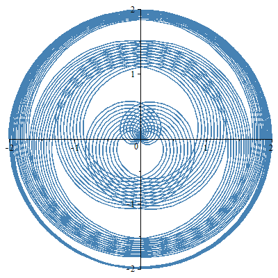
a) $\omega=\zeta(3),t=0..35$.

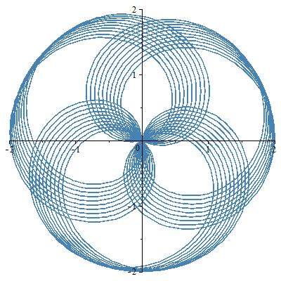
b) $\omega=\pi^{\zeta(3)},t=0..10$.

Figure 1. A piece of the trajectory of $\varphi(t)$ for certain $\omega$’s.

The length of such an interval depends on how good the fraction $\frac{p_{k}}{q_{k}}$ approximates $\omega$. The latter depends on the growth rate of $q_{k}$. So, if $\omega$ is well-approximable, namely $q_{k}$ grows sufficiently fast, then $\varphi(\cdot)$ is similar to a periodic trajectory, during a large, in comparison to the period, time interval. As a result, in many cases the trajectory fills the disk $\mathcal{O}(\varphi)$ in a very lazy manner (see Fig. 1). On the other hand, for a badly approximable $\omega$ the filling is more uniform. Note that the trajectory of $\varphi$ is uniformly distributed with respect to a probability measure $\mu$, independent of $\omega$ (see [1]). The latter means that for all Borel subsets $\mathcal{C}\subset\mathcal{O}(\varphi)$ we have

$$\lim\limits_{T\to+\infty}\frac{1}{2T}\int_{-T}^{T}\mathbf{1}_{\mathcal{C}}(\varphi(t))dt=\mu(C).$$

Thus, such arithmetic properties of $\omega$ affect a character of evolution and not the asymptotic distribution of $\varphi$.

Approximation theorem for almost periodic functions with a similar reasoning extend such phenomena to the case of general almost periodic functions. As well as the measure of irrationality of $\omega$ provides a quantitative information about the dynamic behaviour in the simple case considered above, the Diophantine dimension does this for general almost periodic functions.

References

- [1] Anikushin M. M. Dimension Theory Approach to the Complexity of Almost Periodic Trajectories, International Journal of Evolution Equations, vol. 10, no. 3-4, pp. 215–232, 2017.
- [2] Anikushin M. M. Badly Approximable Numbers and the Growth Rate of the Inclusion Length of an Almost Periodic Function, Proc. of International Student Conference in Saint-Petersburg State University ”SCIENCE AND PROGRESS - 2016”.
- [3] Anikushin M. M., Reitmann V. Development of Concept of Topological Entropy for Systems with Multiple Time, Diff. Equat., vol. 52, no. 13, 2016, pp. 1655–1670. (doi: 10.1134/S0012266116130012)
- [4] J. W. S. Cassels, An Introduction to Diophantine Approximation (Cambridge University Press, 1957).
- [5] Cassels J. W. S., Fröhlich A. Algebraic Number Theory, London: Academic Press, 1986.
- [6] Fukshansky L., Moshchevitin N. On an Effective Variation of Kronecker’s Approximation Theorem Avoiding Algebraic Sets. Proceedings of the American Mathematical Society, DOI: 10.1090/proc/14110
- [7] Katok A., Hasselblatt B. Introduction to the Modern Theory of Dynamical Systems. Cambridge University Press, vol. 54, 1997.
- [8] Khinchin A. Y. Continued Fractions. Dover Publications, New York, 1997.
- [9] Kleinbock D. Y., Margulis G. A. Flows on Homogeneous Spaces and Diophantine Approximation on Manifolds. Annals of Mathematics, pp. 339-360, 1998.
- [10] Lang S. Algebraic Number Theory. Springer-Verlag, 1994.
- [11] Leonov G. A., Kuznetsov N. V., Reitmann V. Attractor Dimension Estimates for Dynamical Systems: Theory and Computation, Springer International Publishing AG, Switzerland, 2018. (in print)
- [12] Moser J. On Commuting Circle Mappings and Simultaneous Diophantine Approximations, Mathematische Zeitschrift. vol. 205, no. 1, pp. 105-121, 1990.
- [13] Naito K. Fractal Dimensions of Almost Periodic Attractors. Ergodic Theory Dyn. Syst., vol. 16, no. 4, 1996, pp. 791–803.
- [14] Pankov A. A. Bounded and Almost Periodic Solutions of Nonlinear Operator Differential Equations. Kluwer Academic Publishers, London, 1990.
- [15] Schmidt W. M. Diophantine Approximation. Springer-Verlag, Berlin, 1980.
- [16] Vorselen T. On Kronecker’s Theorem over the Adles. Master’s thesis, Universiteit Leiden, 2010.