The space of cubic surfaces equipped with a line

Abstract.

The Cayley–Salmon theorem implies the existence of a $27$-sheeted covering space specifying lines contained in smooth cubic surfaces over $\mathbb{C}$. In this paper we compute the rational cohomology of the total space of this cover, using the spectral sequence in the method of simplicial resolution developed by Vassiliev. The covering map is an isomorphism in cohomology (in fact of mixed Hodge structures) and the cohomology ring is isomorphic to that of $\operatorname{PGL}(4,\mathbb{C})$. We derive as a consequence of our theorem that over the finite field $\mathbb{F}_{q}$ the average number of lines on a cubic surface equals $1$ (away from finitely many characteristics); this average is $1+O(q^{-1/2})$ by a standard application of the Weil conjectures.

1. Introduction

One of the first theorems of modern algebraic geometry and specifically enumerative geometry is the Cayley–Salmon theorem [Cay49]. This classical theorem states that every smooth cubic surface (over an algebraically closed field, in particular $\mathbb{C}$) contains exactly $27$ lines. A cubic (hyper)surface in $\mathbb{P}^{3}=\mathbb{C}P^{3}$ is the zero set $S=\mathcal{V}(F)$ of a homogeneous polynomial $F$ of degree $3$ in $4$ variables. The surface $S$ is singular (i.e. not smooth) if and only if the $20$ coefficients of $F$ are a zero of a discriminant polynomial $\Delta\vcentcolon\mathbb{C}^{20}\to\mathbb{C}$. Thus the space of smooth cubic surfaces is an open locus $M=M_{3,3}\vcentcolon=\mathbb{P}^{19}\setminus\mathcal{V}(\Delta)$. The Cayley–Salmon theorem can be reinterpreted as a covering map $\pi\vcentcolon\widetilde{M}\to M$, where $\widetilde{M}$ is the incidence variety of lines and smooth cubic surfaces (see (2.1) and the preceding discussion for precise definitions). The fiber $\pi^{-1}(S)$ over $S\in M$ is the set of $27$ lines on $S$.

The automorphism group of $\mathbb{P}^{3}$ is $\operatorname{PGL}(4,\mathbb{C})$ and this group acts on lines and cubic surfaces, preserving smoothness. In particular the covering map $\pi\vcentcolon\widetilde{M}\to M$ is $\operatorname{PGL}(4,\mathbb{C})$-equivariant. It was shown by Vassiliev (in [Vas99]) that the space $M$ has the same rational cohomology as $\operatorname{PGL}(4,\mathbb{C})$, and it follows from the results of Peters–Steenbrink ([PS03]) that the orbit map given by $g\mapsto g(S_{0})$ induces an isomorphism for any choice of $S_{0}\in M$ (see Theorem 2.4). See also [Tom14].

The main result of this paper is that the covering space $\widetilde{M}$ also has the same rational cohomology.

Theorem 1.1.

For a choice $(S_{0},L_{0})\in\widetilde{M}$, the orbit map $\operatorname{PGL}(4,\mathbb{C})\to\widetilde{M}$ given by $g\mapsto g(S_{0},L_{0})$ induces an isomorphism

$$H^{*}(\widetilde{M};\mathbb{Q})\xrightarrow{\,\smash{\raisebox{-2.58334pt}{$\sim$}}\,}H^{*}(\operatorname{PGL}(4,\mathbb{C});\mathbb{Q})\cong\mathbb{Q}[a_{3},a_{5},a_{7}]/(a_{3}^{2},a_{5}^{2},a_{7}^{2})\,\text{,}$$

where $a_{i}\in H^{i}(\operatorname{PGL}(4,\mathbb{C});\mathbb{Q})$. Since the composition $\operatorname{PGL}(4,\mathbb{C})\to\widetilde{M}\xrightarrow{\pi}M$ also induces an isomorphism on $H^{*}(\_;\mathbb{Q})$, the map

$$\pi^{*}\vcentcolon H^{*}(M;\mathbb{Q})\to H^{*}(\widetilde{M};\mathbb{Q})$$

is an isomorphism. Since the orbit map and $\pi$ are algebraic, the isomorphisms are of mixed Hodge structures.

Remark 1.1.

In particular, $H^{k}(\widetilde{M};\mathbb{Q})$ is pure of Tate type; the generator $a_{2k-1}$ is of bidegree $(k,k)$.

The main tool in our proof of Theorem 1.1 is simplicial resolution à la Vassiliev. However the introduction of a line significantly increases the combinatorics of the casework. We devote all of Section 3 to this computation, while Section 2.2 contains the rest of the proof.

1.1. Applications: moduli space, representations of $W(E_{6})$ and point counts

Before presenting a proof of Theorem 1.1, which we postpone to Section 2.2 and the particularly tedious details further to Section 3, we describe a few applications. All of the corollaries in this section are corollaries to Theorem 1.1.

Cohomology of moduli spaces

The map $\pi\vcentcolon\widetilde{M}\to M$ is $\operatorname{PGL}(4,\mathbb{C})$ equivariant and each orbit (in either $M$ or $\widetilde{M}$) is closed (see e.g. [ACT02]). Thus passing to the geometric quotient we get a covering map

$$\mathcal{H}_{3,3}(1)\to\mathcal{H}_{3,3}\,\text{,}$$

where

$$\mathcal{H}_{3,3}=M/\operatorname{PGL}(4,\mathbb{C})$$

is the moduli space of smooth cubic surfaces and

$$\mathcal{H}_{3,3}(1)=\widetilde{M}/\operatorname{PGL}(4,\mathbb{C})$$

is the moduli space of cubic surfaces equipped with a line. Note that both $\mathcal{H}_{3,3}$ and $\mathcal{H}_{3,3}(1)$ are coarse moduli spaces. For example the Fermat cubic defined by $x^{3}+y^{3}+z^{3}+w^{3}$ equipped with the line $\{x=y,z=w\}$ has non-trivial (but finite) stabilizer in $\operatorname{PGL}(4,\mathbb{C})$. Using [PS03, Theorem 2], which is a generalization of the Leray–Hirsch theorem, we have the following corollary.

Corollary 1.1.

The space $\mathcal{H}_{3,3}(1)$ is $\mathbb{Q}$-acyclic: $H^{i}(\mathcal{H}_{3,3}(1);\mathbb{Q})=0$ for $i>1$.

For comparison, it was already known by Theorem 2.4 that $\mathcal{H}_{3,3}$ is $\mathbb{Q}$-acyclic. Various compactifications of $\mathcal{H}_{3,3}$, $\mathcal{H}_{3,3}(1)$ and other covers can be found in [DvGK05], in particular the two moduli spaces mentioned here are rational. Also relevant are the computation of $\pi_{1}(\mathcal{H}_{3,3})$ (as an orbifold) by Looijenga [Loo08], the identification of a compactification of $\mathcal{H}_{3,3}$ as a quotient of complex hyperbolic $4$-space by Allcock, Carlson and Toledo [ACT02].

The cohomology of the normal cover as a representation of $W(E_{6})$

The combinatorics of how the $27$ lines intersect is extremely well-studied. Let $L$ be the graph with vertices the $27$ lines and edges corresponding to intersecting pairs for the generic cubic surface [Cay49]. It was classically known that the automorphism group of $L$ is realized as the Galois group of the extension given by adjoining the coefficients defining the lines over the field containing the coefficients of a cubic form. Camille Jordan proved [Jor89] that this group is the Weyl group $W(E_{6})$ of the root system $E_{6}$ (see also [Man86, Remark 23.8.2]). The Galois group can also be realized as the monodromy of the covering space $\widetilde{M}\to M$ and hence the deck group of its normal closure; see [Har79].

The cover $\widetilde{M}\to M$ is in fact not normal (Galois): its normal closure is the space $\widetilde{M}_{\text{nor}}$ consisting of pairs $(S,\alpha)$, where $\alpha$ is an identification of the intersection graph of the $27$ lines on $S$ with $L$. The deck group of $\widetilde{M}_{\text{nor}}$ is $W(E_{6})$, as mentioned, and so $H^{*}(\widetilde{M}_{\text{nor}};\mathbb{Q})$ is a $W(E_{6})$ representation. We can restrict this representation to the index-$27$ subgroup that stabilizes a line, which can be identified with $W(D_{5})$ (see [Nar82]). The intermediate cover corresponding to this $W(D_{5})$ is exactly $\widetilde{M}$. We can now deduce the following corollary about $H^{*}(\widetilde{M}_{\text{nor}};\mathbb{Q})$ from Theorem 1.1.

Corollary 1.1.

For any non-trivial irreducible representation $V$ of $W(E_{6})$ appearing in $H^{*}(\widetilde{M}_{\text{nor}};\mathbb{Q})$, the restriction of $V$ to $W(D_{5})$ cannot have a trivial summand. Equivalently, the non-trivial irreducible representations of $W(E_{6})$ that occur in the $27$-dimensional permutation representation given by the action on left cosets of $W(D_{5})$ in $W(E_{6})$ cannot occur in $H^{*}(\widetilde{M}_{\text{nor}};\mathbb{Q})$.

Proof.

By Theorem 1.1 and transfer,

$$H^{*}(\widetilde{M}_{\text{nor}};\mathbb{Q})^{W(E_{6})}=H^{*}(M;\mathbb{Q})=H^{*}(\widetilde{M};\mathbb{Q})=H^{*}(\widetilde{M}_{\text{nor}};\mathbb{Q})^{W(D_{5})}\,\text{.}$$

The second statement is equivalent to the first by Frobenius reciprocity. ∎

Computing the cohomology $H^{*}(\widetilde{M}_{\text{nor}};\mathbb{Q})$ (as a $W(E_{6})$ representation) would be an obvious and major generalization of Theorem 1.1. While the above corollary provides a restriction towards which irreducible representations can occur, it only rules out a small fraction: the order of $W(E_{6})$ is $51840$, and it has $24$ non-trivial irreducible representations (see [Car85, 428–429] for a character table).

There are other intermediate covers of $M$, by marking different configurations of the $27$ lines. For instance, taking unordered triples of lines that intersect pairwise, we get a $45$-sheeted cover marking the ‘tritangents’ of a cubic surface. See [Nar82] and the appendix by Looijenga for more on this cover and its quotient under $\operatorname{PGL}(4,\mathbb{C})$.

Lines over $\mathbb{F}_{q}$

The spaces $\widetilde{M}$ and $M$ as defined above are (the complex points of) quasiprojective varieties defined by integer polynomials. To be more explicit, the discriminant $\Delta$ is an integer polynomial, as are the polynomials defining the incidence of a line and a cubic surface. For a finite field $\mathbb{F}_{q}$ of characteristic $p$, we can base change to $\mathbb{F}_{q}$. That is, reducing the defining polynomials $\operatorname{mod}p$ defines spaces

$$M(\mathbb{F}_{q})\subset\mathbb{P}^{19}(\mathbb{F}_{q})\,\text{,}$$

$$\widetilde{M}(\mathbb{F}_{q})\subset\mathbb{P}^{19}(\mathbb{F}_{q})\times\mathrm{Gr}(2,4)(\mathbb{F}_{q})\,\text{,}$$

and a projection map

$$\pi\vcentcolon\widetilde{M}(\mathbb{F}_{q})\to M(\mathbb{F}_{q})\,\text{.}$$

For $p\neq 3$, the discriminant $\Delta$ continues to characterize singular polynomials, so $M(\mathbb{F}_{q})$ is the space of smooth cubic surfaces defined over $\mathbb{F}_{q}$ (where a homogeneous cubic polynomial is smooth if it is smooth at all $\mkern 1.5mu\overline{\mkern-1.5mu\mathbb{F}_{q}\mkern-1.5mu}\mkern 1.5mu$ points). Similarly, $\widetilde{M}(\mathbb{F}_{q})$ is the space of pairs $(S,L)$ of smooth cubic surfaces $S$ and lines $L$ defined over $\mathbb{F}_{q}$ such that $L\subset S$. Thus, $\dfrac{\#\widetilde{M}(\mathbb{F}_{q})}{\#M(\mathbb{F}_{q})}$ is the average number of $\mathbb{F}_{q}$-lines on a cubic surface defined over $\mathbb{F}_{q}$. The Grothendieck–Lefschetz fixed point formula (see e.g. [Mil13]) lets us use our results to deduce consequences about the cardinality of $\#\widetilde{M}(\mathbb{F}_{q})$.

Remark 1.1.

The fact that $\widetilde{M}$ is a connected cover of $M$ already implies $H^{0}(\widetilde{M};\mathbb{Q})\cong\mathbb{Q}$. Given Deligne’s theorem [Del80, Théorème 3.3.1] we get that both $\#M(\mathbb{F}_{q})$ and $\#\widetilde{M}(\mathbb{F}_{q})$ are $q^{19}(1+O(q^{-1/2}))$, since $\dim M=\dim\widetilde{M}=19$. Hence the average number of lines on a $\mathbb{F}_{q}$-cubic surface is $1+O(q^{-1/2})$ as $q\to\infty$. One needs much more information to compute this number exactly.

Corollary 1.1.

There is a finite set of characteristics, so that for a fixed $q$ with $p$ not in this set,

$$\#M(\mathbb{F}_{q})=\#\widetilde{M}(\mathbb{F}_{q})=q^{4}(\#\operatorname{PGL}(4,\mathbb{F}_{q}))=q^{4}\frac{(q^{4}-1)(q^{4}-q)(q^{4}-q^{2})(q^{4}-q)}{q-1}\,\text{.}$$

Thus the average number of lines defined over $\mathbb{F}_{q}$ on a smooth cubic surface defined over $\mathbb{F}_{q}$ is exactly $1$.

To the best of our knowledge, the point count for $\widetilde{M}(\mathbb{F}_{q})$ and the consequence about the average number of lines is new.

Proof of Section 1.1.

The varieties $M$ and $\widetilde{M}$ are smooth since $M$ is open in $\mathbb{P}^{19}$. For a smooth quasiprojective variety $Y$, the $\mathbb{F}_{q}$ points are exactly the fixed points of $\operatorname{Frob}_{q}$ on $Y(\mkern 1.5mu\overline{\mkern-1.5mu\mathbb{F}_{q}\mkern-1.5mu}\mkern 1.5mu)$, and $\#Y(\mathbb{F}_{q})$ is determined by the Grothendieck–Lefschetz fixed point formula (see e.g. [Mil13]):

$$\#Y(\mathbb{F}_{q})=q^{\dim Y}\sum_{i\geq 0}(-1)^{i}\operatorname{Tr}(\operatorname{Frob}_{q}\vcentcolon H^{i}_{\text{ét}}(Y;\mathbb{Q}_{\ell})^{\vee})\,\text{,}$$

where $\ell$ is a prime other than $p$. Further, there are comparison theorems implying isomorphisms

$$H^{i}_{\text{ét}}(Y;\mathbb{Q}_{\ell})\cong H^{i}(Y(\mathbb{C});\mathbb{Q}_{\ell})\cong H^{i}(Y(\mathbb{C});\mathbb{Q})\otimes\mathbb{Q}_{\ell}\,\text{,}$$

away from a finite set of characteristics (see e.g. [Del77, Théorème 1.4.6.3, Théorème 7.1.9]). In particular, as a corollary of Theorem 1.1 we obtain $\#\widetilde{M}(\mathbb{F}_{q})=\#M(\mathbb{F}_{q})=q^{4}(\#\operatorname{PGL}(4,\mathbb{F}_{q}))$ and hence the corollary. ∎

Remark 1.1.

One can define $\mathcal{H}_{3,3}(\mathbb{F}_{q})$ and $\mathcal{H}_{3,3}(1)(\mathbb{F}_{q})$ as base-changes of $\mathcal{H}_{3,3}$ and $\mathcal{H}_{3,3}(1)$ from above. Using an analogue of the Groethendieck–Lefschetz fixed-point formula, it is possible to conclude that

$$\#\mathcal{H}_{3,3}(1)(\mathbb{F}_{q})=\#\mathcal{H}_{3,3}(\mathbb{F}_{q})=q^{4}\,\text{,}$$

although one needs to be more careful in interpreting these ‘point counts’ mean. However, a deeper discussion of the arguments involved is out of the scope of this paper.

1.2. Acknowledgments

I would like to thank Benson Farb for his invaluable advice and comments throughout the composition of this paper and also for suggesting the problem. I am also grateful to Weiyan Chen, Nir Gadish, Sean Howe and Akhil Mathew for many helpful conversations. I am grateful to Igor Dolgachev for pointing me towards some existing results about moduli spaces of cubic surfaces. Finally, I would like to thank Maxime Bergeron, Priyavrat Deshpande, Eduard Looijenga and Jesse Wolfson for their helpful comments to make the paper more readable.

2. Rational cohomology of the incidence variety

2.1. Definitions and setup

From now on we will work over the field $\mathbb{C}$ of complex numbers. Let $X=X_{3,3}$ be the space of smooth homogeneous degree $3$ (complex) polynomials over $4$ variables, for concreteness a subset of $\mathbb{C}[x,y,z,w]_{3}\cong\mathbb{C}^{20}$. A polynomial $F\in\mathbb{C}[x,y,z,w]_{3}$ is smooth precisely when $\{F_{x},F_{y},F_{z},F_{w}\}$ do not have a common root, by Euler’s formula. This is equivalent to a certain ‘discriminant’ in the coefficients not vanishing; there is a polynomial $\Delta\vcentcolon\mathbb{C}^{20}\to\mathbb{C}$ with integer coefficients that vanishes on (the coefficients of) $F$ if and only if $F$ is not smooth. In other words, $X$ is the complement of the discriminant locus, $\Sigma=\mathcal{V}(\Delta)\subset\mathbb{C}^{20}$.

We also have the ‘incidence variety’ of a line and a (not necessarily smooth) cubic polynomial

$$\Pi=\left\{(F,L)\mathrel{}\middle|\mathrel{}F|_{L}\equiv 0\right\}\subset\mathbb{C}[x,y,z,w]_{3}\times\mathrm{Gr}(2,4)\,\text{,}$$

where $\mathrm{Gr}(2,4)$ is the Grassmannian of lines in $\mathbb{P}^{3}$ (that is, $2$-planes in $\mathbb{C}^{4}$). This space comes equipped with two projections. The first, $\pi\vcentcolon(F,L)\mapsto F$ forgets the line, and we denote the inverse image $\pi^{-1}(X)$ of $X$ by $\widetilde{X}$, which by (a version of) the Cayley–Salmon theorem is a $27$-sheeted cover $\pi\vcentcolon\widetilde{X}\to X$.

The second projection is to $\mathrm{Gr}(2,4)$, given by $(F,L)\mapsto L$, and is a fiber bundle with fiber $\Pi_{\ell}\cong\mathbb{C}^{16}$ over $\ell\in\mathrm{Gr}(2,4)$. To be explicit, $\Pi_{\ell}$ is the space of (not necessarily smooth) cubic polynomials that vanish on $\ell$. The restriction of the projection to $\widetilde{X}$ is also a fiber bundle, and we will denote the fiber over $\ell$ by $\widetilde{X}_{\ell}$, this is the space of smooth homogeneous cubic polynomials in $4$ variables that vanish on $\ell$. Let

$$\Sigma_{\ell}=\Pi_{\ell}\setminus\widetilde{X}_{\ell}=\Sigma\cap\Pi_{\ell}\,\text{.}$$

To go from the space of polynomials to the space of cubic surfaces, we need to quotient by the action of $\mathbb{C}^{\times}$. Namely, given a homogeneous cubic polynomial $F$ and $\lambda\in\mathbb{C}^{\times}$, the product $\lambda F$ is another homogeneous cubic polynomial which defines the same surface $\mathcal{V}(F)=\mathcal{V}(\lambda F)$ and $F$ is smooth if and only if $\lambda F$ is. Alternatively viewed, $\Delta$ is a homogeneous polynomial and $\Sigma$ is a conical hypersurface in $\mathbb{C}^{20}$, so passing to the quotient by $\mathbb{C}^{\times}$ produces spaces

$$M=X_{3,3}/\mathbb{C}^{\times}\subset\mathbb{P}^{19}\,\text{,}$$

(2.1) $$\widetilde{M}=\widetilde{X}/\mathbb{C}^{\times}\subset M\times\mathrm{Gr}(2,4)$$

and a covering map $\widetilde{M}\to M$, which we will also denote by $\pi$.

The map $\widetilde{M}\to\mathrm{Gr}(2,4)$ continues to be a fiber bundle, we denote the fiber over $\ell\in\mathrm{Gr}(2,4)$ by

$$\widetilde{M}_{\ell}=\left\{(S,\ell)\mathrel{}\middle|\mathrel{}S\in M,S\supset\ell\right\}\,\text{.}$$

All these spaces and the maps described so far fit into the following (somewhat clumsy) commuting diagram:

(2.2)

There is one more action to consider, which is important for both our theorem and its proof. As mentioned in the introduction, $\operatorname{GL}(4)\vcentcolon=\operatorname{GL}(4,\mathbb{C})$ acts on $\mathbb{C}^{4}$ and $\operatorname{PGL}(4)=\operatorname{GL}(4)/(\mathbb{C}^{\times}I)$ acts on the quotient $\mathbb{P}^{3}$. There are induced actions on the spaces defined above: on $X$ and $\widetilde{X}$ by $\operatorname{GL}(4)$; on $M$ and $\widetilde{M}$ by $\operatorname{PGL}(4)$. The action of $\operatorname{GL}(4)$ on $\mathrm{Gr}(2,4)$ also factors through $\operatorname{PGL}(4)$. Fixing a line $\ell\in\mathrm{Gr}(2,4)$, the respective stabilizers in $\operatorname{GL}(4)$ and $\operatorname{PGL}(4)$ act on the fibers $\widetilde{X}_{\ell}$ and $\widetilde{M}_{\ell}$. If we fix a basepoint $(F_{0},L_{0})\in\widetilde{X}$, and set $S_{0}=\mathcal{V}(F_{0})$ so that $(S_{0},L_{0})\in\widetilde{M}$, we get orbit maps $g\mapsto g(S_{0},L_{0})=(g\cdot S_{0},g\cdot L_{0})$, and so on. Then we also have the following commuting diagram:

(2.3)

All the four maps in the bottom-left square are in fact maps of bundles over the same base $\mathrm{Gr}(2,4)$, and all the vertical maps are bundles with fiber $\mathbb{C}^{\times}$. The second and third vertical maps are elaborated in the previous diagram (2.2).

Remark 2.3.

It is worth noting that the map on the fibers $\mathbb{C}^{\times}\to\mathbb{C}^{\times}$ induced by the first horizontal map is not identity, the matrix $\omega I$ acts by $\omega^{3}=1$ on a cubic polynomial $F$. As indicated, it is the degree $3$ map $z\mapsto z^{3}$, which is an isomorphism with rational coefficients, so this does not affect our computations.

Remark 2.3.

Since $\widetilde{M}$ is connected, the orbit maps for different choices of basepoint $(S_{0},L_{0})\in\widetilde{M}$ are homotopic.

As mentioned in the introduction, Vassiliev’s results imply that $M$ and $\operatorname{PGL}(4)$ have the same rational cohomology.

Theorem 2.4 (Vassiliev [Vas99], Peters–Steenbrink [PS03]).

The map $\operatorname{PGL}(4)\to M$ given by $g\mapsto g(S_{0})$ induces an isomorphism

$$H^{*}(M;\mathbb{Q})\xrightarrow{\,\smash{\raisebox{-2.58334pt}{$\sim$}}\,}H^{*}(\operatorname{PGL}(4);\mathbb{Q})\,\text{.}$$

By transfer we know that $\pi^{*}\vcentcolon H^{*}(M;\mathbb{Q})\to H^{*}(\widetilde{M};\mathbb{Q})$ is an injection. This also follows from the fact that the orbit map in the above theorem factors through $\widetilde{M}$. In fact, there is no new cohomology that appears in this cover, as in Theorem 1.1.

2.2. Proof of Theorem 1.1 and the role of simplicial resolution

Vassiliev’s method of simplicial resolution works by first reducing the computation of the cohomology of the discriminant complement $X$ to computing the (Borel–Moore) homology of the discriminant locus $\Sigma$ via Alexander duality. The space $\Sigma$ consisting of the singular cubic surfaces is itself highly singular, and stratifies based on the how big the singular set of each $F\in\Sigma$ is. Applying the spectral sequence of a filtration to this stratification produces a spectral sequence converging to $\mkern 1.5mu\overline{\mkern-1.5muH\mkern-1.5mu}\mkern 1.5mu_{*}(\Sigma)=H_{*}^{\mathrm{BM}}(\Sigma)$ (Borel–Moore or compactly supported homology).

While $\widetilde{M}$ or $\widetilde{X}$ is not an open subset of a vector space, recall that the fiber $\widetilde{X}_{\ell}$ over $\ell$ of the map $\widetilde{X}\to\mathrm{Gr}(2,4)$ is open in the vector space $\Pi_{\ell}$ of polynomials vanishing on $\ell$. So we can apply the Vassiliev spectral sequence to each $\widetilde{X}_{\ell}$ to find $H^{*}(\widetilde{X}_{\ell};\mathbb{Q})$. For this, we need to stratify $\Sigma_{\ell}=\Sigma\cap\Pi_{\ell}$ by not just how big the singular sets are, but how they are configured with respect to the line $\ell$. These are the types and subtypes described in Section 3.1. For now we will assume that we can perform this computation (which takes up all of Section 3), and when needed we refer to the answer described in Section 3.3.

Lemma 2.4.

Let $f\vcentcolon\mathbb{C}^{n}\to\mathbb{C}$ be a non-constant homogeneous polynomial of degree $d$, so that $\mathcal{V}(f)$ is a conical hypersurface; let its complement be $Y=\mathbb{C}^{n}\setminus\mathcal{V}(f)$. Let $\mathbb{P}Y=Y/\mathbb{C}^{\times}=\mathbb{P}^{n-1}\setminus\mathcal{V}_{\mathbb{P}}(f)$ be the complement of the projective hypersurface given by the same polynomial $f$. Then $H^{*}(Y;\mathbb{Q})\cong H^{*}(\mathbb{C}^{\times})\otimes H^{*}(\mathbb{P}Y)$.

Proof.

We have a fiber bundle

and for any fiber $\mathbb{C}^{\times}a$, the map $\mathbb{C}^{\times}a\hookrightarrow Y\xrightarrow{f}\mathbb{C}^{\times}$ is given by $\lambda\mapsto\lambda^{d}f(a)$, which is degree $d\neq 0$ on $\mathbb{C}^{\times}$ and hence an isomorphism on $H^{*}(\mathbb{C}^{\times};\mathbb{Q})$. This implies the conclusion by the Leray–Hirsch theorem. ∎

Lemma 2.4.

For a fixed $\ell\in\mathrm{Gr}(2,4)$, let $\operatorname{Stab}_{\operatorname{GL}(4)}(\ell)$ be the stabilizer of $\ell$ in $\operatorname{GL}(4)$. Then for a choice of basepoint $F_{0}\in\widetilde{X}_{\ell}$, the orbit map $\operatorname{Stab}(\ell)\to\widetilde{X}_{\ell}$ given by $g\mapsto g(F_{0})=F_{0}\circ g$ induces a surjection

$$H^{*}(\widetilde{X}_{\ell};\mathbb{Q})\twoheadrightarrow H^{*}(\operatorname{Stab}_{\operatorname{GL}(4)}(\ell);\mathbb{Q})\cong H^{*}(\operatorname{GL}(2)\times\operatorname{GL}(2);\mathbb{Q})\,\text{.}$$

Proof.

First, fix a complement $\ell^{\perp}$ of $\ell$ (as the notation suggests, we can pick the orthogonal complement of $\ell$). Then $\operatorname{Stab}_{\operatorname{GL}(4)}(\ell)$ deformation retracts to $G=\operatorname{Stab}_{\operatorname{GL}(4)}(\ell,\ell^{\perp})$ (the elements that fix both $\ell$ and $\ell^{\perp}$). Further,

$$G=\operatorname{GL}(\ell)\times\operatorname{GL}(\ell^{\perp})\,\text{.}$$

As in the computation of $H^{*}(\widetilde{X}_{\ell};\mathbb{Q})$ in Section 3, it is important to identify via Alexander duality $H^{*}(\widetilde{X}_{\ell};\mathbb{Q})$ with $\mkern 1.5mu\overline{\mkern-1.5muH\mkern-1.5mu}\mkern 1.5mu_{*}(\Sigma_{\ell})$, and similarly $H^{*}(\operatorname{GL}(2);\mathbb{Q})$ with $\mkern 1.5mu\overline{\mkern-1.5muH\mkern-1.5mu}\mkern 1.5mu_{*}(\operatorname{Mat}(2)\setminus\operatorname{GL}(2))$, where $\operatorname{Mat}(2)$ is the space of all $2\times 2$ matrices. The generators of $H^{*}(\operatorname{GL}(2);\mathbb{Q})$ (as a ring) are represented by the locus of matrices whose first $i$ columns are linearly dependent, for $i=1,2$.

Fix $P\in\ell$ and $P^{\prime}\in\ell^{\perp}$ non-zero and extend to bases of $\ell$ and $\ell^{\perp}$ respectively. This identifies $\operatorname{GL}(\ell)\times\operatorname{GL}(\ell^{\perp})\cong\operatorname{GL}(2)\times\operatorname{GL}(2)$. The orbit map extends to a map

$$\operatorname{Mat}(2)\times\operatorname{Mat}(2)\to\Pi_{\ell}=\widetilde{X}_{\ell}\cup\Sigma_{\ell}\,\text{.}$$

It is enough to identify subspaces of $\Sigma_{\ell}$ that pull-back to (a rational multiple of) the corresponding subspaces of $\operatorname{Mat}(2)\times\operatorname{Mat}(2)$. Then directly from arguments in [PS03, section 6], it is enough to pick the following four subspaces of polynomials that are: (i) singular at $P$, (ii) singular at some (non-zero) point of $\ell$, (iii) singular at $P^{\prime}$, (iv) singular at some (non-zero) point of $\ell^{\perp}$. ∎

Now we prove the analogue of Theorem 1.1 before projectivization.

Proposition 2.4.

The orbit map $\operatorname{GL}(4)\to\widetilde{X}$ and the projection $\pi\vcentcolon\widetilde{X}\to X$ induce isomorphisms

$$H^{*}(X;\mathbb{Q})\xrightarrow{\,\smash{\raisebox{-2.58334pt}{$\sim$}}\,}H^{*}(\widetilde{X};\mathbb{Q})\xrightarrow{\,\smash{\raisebox{-2.58334pt}{$\sim$}}\,}H^{*}(\operatorname{GL}(4);\mathbb{Q})\,\text{.}$$

Proof.

Note that by Section 3.3,

$$H^{*}(\widetilde{X}_{\ell};\mathbb{Q})\cong H^{*}(\operatorname{GL}(2)\times\operatorname{GL}(2);\mathbb{Q})\cong H^{*}(\operatorname{Stab}_{\operatorname{GL}(4)}(\ell);\mathbb{Q})\,\text{.}$$

Since the orbit map $\operatorname{Stab}_{\operatorname{GL}(4)}(\ell)\to\widetilde{X}_{\ell}$ induces a surjection on $H^{*}(\_;\mathbb{Q})$ by Section 2.2, the induced map must be an isomorphism.

Thus we have a map of bundles (as in (2.2))

that fiberwise induces an isomorphism

$$H^{*}(\widetilde{X}_{\ell};\mathbb{Q})\xrightarrow{\,\smash{\raisebox{-2.58334pt}{$\sim$}}\,}H^{*}(\operatorname{Stab}_{\operatorname{GL}(4)}(\ell);\mathbb{Q})\,\text{.}$$

There is no monodromy in either bundle since $\mathrm{Gr}(2,4)$ is simply connected. Therefore from naturality of the Serre spectral sequence, the map $\operatorname{GL}(4)\to\widetilde{X}$ must also be an isomorphism on cohomology. ∎

Converting this to a proof of Theorem 1.1 is fairly simple. We restate the theorem here for convenience. See 1.1

Proof of Theorem 1.1.

We have another map of bundles (as in (2.3)):

By Section 2.2, both of these bundles satisfy the Leray–Hirsch theorem and the fiberwise map $\mathbb{C}^{\times}\to\mathbb{C}^{\times}$ is degree $3$, so induces an isomorphism on $H^{*}(\mathbb{C}^{\times};\mathbb{Q})$. Thus the map of bases $\operatorname{PGL}(4)\to\widetilde{M}$ must also induce an isomorphism

$$H^{*}(\widetilde{M};\mathbb{Q})\xrightarrow{\,\smash{\raisebox{-2.58334pt}{$\sim$}}\,}H^{*}(\operatorname{PGL}(4);\mathbb{Q})\,\text{.}\qed$$

3. Rational cohomology of $\widetilde{X}_{\ell}$

3.1. Definitions and plan of attack

We will suppress constant rational coefficients throughout this section, and use $\mkern 1.5mu\overline{\mkern-1.5muH\mkern-1.5mu}\mkern 1.5mu$ to denote Borel–Moore homology (also with rational coefficients by default). Note that for an orientable but not necessarily compact $2n$-manifold $M$, Poincaré duality takes the form

$$\mkern 1.5mu\overline{\mkern-1.5muH\mkern-1.5mu}\mkern 1.5mu_{i}(M)\cong H^{2n-i}(M)\cong(H_{2n-i}(M))^{\vee}\cong(H^{i}_{c}(M))^{\vee}\,\text{.}$$

We use the spectral sequence developed by Vassiliev in [Vas99]. We refer the reader to Vassiliev’s paper for the theory, but summarize how the computation works in practice. Recall that $\widetilde{X}_{\ell}\subset\Pi_{\ell}\cong\mathbb{C}^{16}$, and set $\Sigma_{\ell}=\Pi_{\ell}\setminus\widetilde{X}_{\ell}=\Pi_{\ell}\cap\Sigma$, the set of singular cubic polynomials that vanish on the line $\ell$. Then via Alexander duality,

(3.1) $$\widetilde{H}^{i}(\widetilde{X}_{\ell})=\mkern 1.5mu\overline{\mkern-1.5muH\mkern-1.5mu}\mkern 1.5mu_{31-i}(\Sigma_{\ell})\,\text{.}$$

Note that $\Sigma_{\ell}$ is a hypersurface in $\Pi_{\ell}$, being the vanishing locus of $\Delta_{\ell}=\Delta|_{\Pi_{\ell}}$.

Remark 3.1.

The complex variety $\widetilde{X}_{\ell}$, being the complement of a hypersurface, is affine and hence a $16$-dimensional Stein manifold. Thus by the Andreotti–Frankel theorem, $H^{i}(\widetilde{X}_{\ell})=0$ for $i>16$. This along with Eq. 3.1 imply that $\mkern 1.5mu\overline{\mkern-1.5muH\mkern-1.5mu}\mkern 1.5mu_{i}(\Sigma_{\ell})$ can only be non-zero for $15\leq i\leq 31$.

Let $F\in\Sigma_{\ell}$ be a singular cubic polynomial and let $K$ be its singular locus. Then $K$, as a subset of $\mathbb{P}^{3}$, can be one of the following $11$ types (see [Vas99, Proposition 8]):

1. a point;

2. two distinct points;

3. a line;

4. three points, not on a line;

5. a smooth conic contained in a plane $\mathbb{P}^{2}\subset\mathbb{P}^{3}$;

6. a pair of intersecting lines;

7. four points, not on a plane;

8. a plane;

9. three lines through a point, not all on the same plane;

10. a smooth conic contained in a plane along with another point not on that plane;

11. all of $\mathbb{P}^{3}$ .

These further break up as subtypes depending on their configuration with respect to $\ell$. For most of the types, how they break up will not be relevant to us; we list those that will. We list names for the points for convenience, they are still to be thought of as a priori unordered sets of points: $\{P,Q\}=\{Q,P\}$ and so on.

1. a point $P$

   1. $P\in\ell$

   2. $P\notin\ell$

2. two points $P$, $Q$

   1. $P,Q\in\ell$

   2. $P\in\ell$, $Q\notin\ell$

   3. $P,Q\notin\ell$, $P$ and $Q$ coplanar with $\ell$

   4. $P,Q\notin\ell$, $P$ and $Q$ not coplanar with $\ell$

3. three points $P$, $Q$, $R$, not collinear

   1. $P,Q\in\ell$, $R\notin\ell$

   2. $P\in\ell$, $Q,R\notin\ell$, $Q$, $R$ coplanar with $\ell$

   3. $P\in\ell$, $Q,R\notin\ell$, $Q$, $R$ not coplanar with $\ell$

   4. $P,Q,R\notin\ell$, $P$, $Q$, $R$ and $\ell$ all coplanar

   5. $P,Q,R\notin\ell$, $P$, $Q$ and $\ell$ coplanar, $R$ not on that plane

   6. $P,Q,R\notin\ell$, no two coplanar with $\ell$

4. four points $P$, $Q$, $R$, $S$, not coplanar

   1. $P,Q\in\ell$, $R,S\notin\ell$

   2. $P\in\ell$, $Q,R,S\notin\ell$, $Q$, $R$, $\ell$ coplanar

   3. $P\in\ell$, no two of $Q$, $R$, $S$ coplanar with $\ell$

   4. $P,Q,R,S\notin\ell$, $P$, $Q$, $R$ coplanar with $\ell$, but $S$ not on that plane

   5. $P,Q,R,S\notin\ell$, $P$, $Q$ and $\ell$ coplanar, $R$, $S$ and $\ell$ coplanar

   6. $P,Q,R,S\notin\ell$, $P$, $Q$ and $\ell$ coplanar, no other pair coplanar with $\ell$

   7. $P,Q,R,S\notin\ell$, no two coplanar with $\ell$

Remark 3.1.

The types correspond to orbits of the singular loci under the $\operatorname{PGL}(4)$ action on $\mathbb{P}^{3}$ and the subtypes correspond to orbits under $\operatorname{Stab}(\ell)\subset\operatorname{PGL}(4)$, but this will not be explicitly important for us.

Definition 3.1.

For a manifold $M$ and natural number $n$, the ordered configuration space of $n$ points on $M$ is given by

$$\operatorname{PConf}_{n}(M)\vcentcolon=\{(a_{1},\dots,a_{n})\in M^{n}\mid a_{i}\neq a_{j}\text{ for }i\neq j\}\,\text{.}$$

This space comes with a natural action of the symmetric group $\mathfrak{S}_{n}$ by permuting the coordinates and the quotient is the unordered configuration space $\operatorname{UConf}_{n}(M)$ of $n$ points on $M$.

Definition 3.1.

For any $A\subseteq\operatorname{UConf}_{n}(M)$, the sign local coefficients on $A$, denoted by $\pm\mathbb{Q}$, is given by the composition

$$\pi_{1}(A)\to\pi_{1}(\operatorname{UConf}_{n}(M))\to\mathfrak{S}_{n}\to\{\pm 1\}\subset\mathbb{Q}^{\times}$$

thought of as a representation on $\mathbb{Q}$. Explicitly, a loop in $A$ acts on $\mathbb{Q}$ by the sign of the induced permutation on the $n$ points.

The method of simplicial resolution produces for us a space $\sigma$ with a map $f\vcentcolon\sigma\to\Sigma_{\ell}$ with the following properties:

1. The map $f_{*}\vcentcolon\mkern 1.5mu\overline{\mkern-1.5muH\mkern-1.5mu}\mkern 1.5mu_{*}(\sigma)\to\mkern 1.5mu\overline{\mkern-1.5muH\mkern-1.5mu}\mkern 1.5mu_{*}(\Sigma_{\ell})$ is an isomorphism.

2. The space $\sigma$ has a stratification

   $$\sigma=\bigcup_{i}F_{i}\,\text{,}$$

   where $i$ varies over all the subtypes (not just the ones listed, but all of them). That is, $F_{i}$ is a stratum corresponding to the subtype $i$. The strata are (partially) ordered by degeneracy: $F_{i}$ intersects $\mkern 1.5mu\overline{\mkern-1.5muF_{j}\mkern-1.5mu}\mkern 1.5mu$ only if polynomials with singularity of subtype $i$ can degenerate to a polynomial with singularity of subtype $j$.

3. Let

   $$A_{i}=\{\text{singular sets $K$ of subtype~{}$i$}\}$$

   and $K\in A_{i}$. Let $L(K)$ be the linear subspace of $\Pi_{\ell}$ consisting of polynomials that are singular on $K$ and possibly elsewhere. Then there are spaces $\Phi_{i}$ and $\Lambda(K)$ along with fiber bundles:

4. The space $\Lambda(K)$ is an open cone with vertex representing $K$ and captures the combinatorics and topology of the subsets of $K$ that can appear as singular sets of other polynomials in $\Sigma_{\ell}$. The homeomorphism type of $\Lambda(K)$ depends only on the type of $K$ and not its subtype. Further, $\mkern 1.5mu\overline{\mkern-1.5muH\mkern-1.5mu}\mkern 1.5mu_{*}(\Lambda(K))=0$ unless $K$ is of type I, II, IV, VII or XI. For $K$ of type I, II, IV and VII respectively, i.e. when $K$ is a finite set of points, $\Lambda(K)$ can be identified with the open simplex with vertex set $K$. In particular, setting $n=\#K$,

   $$\mkern 1.5mu\overline{\mkern-1.5muH\mkern-1.5mu}\mkern 1.5mu_{*}(\Lambda(K))=0\text{ for }*\neq n-1\,\text{,}$$

   and

   $$\mkern 1.5mu\overline{\mkern-1.5muH\mkern-1.5mu}\mkern 1.5mu_{n-1}(\Lambda(K))\cong\mathbb{Q}\,\text{,}$$

   generated by the fundamental class representing an orientation on the simplex $\Lambda(K)\cong B^{n-1}$. Further, $A_{i}$ is a subset of $\operatorname{UConf}_{n}(\mathbb{P}^{3})$, and the monodromy on $\mkern 1.5mu\overline{\mkern-1.5muH\mkern-1.5mu}\mkern 1.5mu_{*}(\Lambda(K))$ is given by $\pm\mathbb{Q}$ (permuting the points of $K$ changes the orientation of the simplex by the sign of the permutation).

5. For the type XI (note that XI has only one subtype, itself), $A$ is singleton, the only element being $K=\mathbb{P}^{3}$. The only polynomial singular on $K$ is $0$, so $L(K)=\{0\}$. Thus $F=\Phi=\Lambda(\mathbb{P}^{3})$. Further, the space $\Phi=\Lambda(\mathbb{P}^{3})$ is the open cone over $\bigcup_{j\neq}\Phi_{j}$ for certain gluings.

Example 3.1.

For the subtype two-pointsb, a point on $\ell$ and a point not on $\ell$, we have $A=\ell\times\mathbb{P}^{3}\setminus\ell$. For the subtype two-pointsd, two points not coplanar with $\ell$, the space $A$ is an open set in $\operatorname{UConf}_{2}(\mathbb{P}^{3}\setminus\ell)$.

We refer the reader to [Vas99] for details of the construction and proofs for (1)–(5). Everything we use for our computation has been summarized in these properties. We now go through the steps of the computation before digging into the details.

By the isomorphism given by Alexander duality (Eq. 3.1), we are reduced to computing $\mkern 1.5mu\overline{\mkern-1.5muH\mkern-1.5mu}\mkern 1.5mu_{*}(\Sigma_{\ell})$. By (1), this is the same as $\mkern 1.5mu\overline{\mkern-1.5muH\mkern-1.5mu}\mkern 1.5mu_{*}(\sigma)$. Let

$$\deg(i)=14-\dim L(K)$$

for any $K\in A_{i}$. This is monotonic on the poset described in (2), in the sense that if $F_{i}$ intersects $\mkern 1.5mu\overline{\mkern-1.5muF_{j}\mkern-1.5mu}\mkern 1.5mu$, then $\deg(i)\leq\deg(j)$. Using the filtration of $\sigma$ given by $\bigcup_{\deg(i)\leq p}F_{i}$ there is a spectral sequence $E^{r}_{p,q}\implies\mkern 1.5mu\overline{\mkern-1.5muH\mkern-1.5mu}\mkern 1.5mu_{p+q}\sigma$, with the $E^{1}$ page given by

(3.2) $$E^{1}_{p,q}=\bigoplus_{\deg(i)=p}\mkern 1.5mu\overline{\mkern-1.5muH\mkern-1.5mu}\mkern 1.5mu_{p+q}(F_{i})\,\text{.}$$

To compute each term, since $L(K)\to F_{i}\to\Phi_{i}$ is a complex vector bundle, we have the Thom isomorphism

(3.3) $$\mkern 1.5mu\overline{\mkern-1.5muH\mkern-1.5mu}\mkern 1.5mu_{*}(F_{i})=\mkern 1.5mu\overline{\mkern-1.5muH\mkern-1.5mu}\mkern 1.5mu_{*-2\dim_{\mathbb{C}}L(K)}(\Phi_{i})\,\text{.}$$

For the right-hand side, if $\Lambda(K)$ is acyclic then so must be $\Phi_{i}$, so this automatically vanishes unless $i$ is a subtype of I, II, IV, VII, or XI.

For the (sub)type XI, from (5) we have that $\Phi=CZ$, the open cone on $Z$, where

$$Z=\bigcup_{i\neq}\Phi_{i}\,\text{.}$$

So we get a spectral sequence $e^{r}_{p,q}\implies H_{p+q}(Z)$ with

$$e^{1}_{p,q}=\bigoplus_{\begin{subarray}{c}\deg(j)=p,\\ j\neq\end{subarray}}\mkern 1.5mu\overline{\mkern-1.5muH\mkern-1.5mu}\mkern 1.5mu_{p+q}(\Phi_{j})\,\text{.}$$

But then we also have

$$\mkern 1.5mu\overline{\mkern-1.5muH\mkern-1.5mu}\mkern 1.5mu_{*}(CZ)=H_{*}(CZ,Z)=\widetilde{H}_{*-1}(Z)\,\text{.}$$

For all the other $i$, the set $K$ is finite, of say $n$ points ($1\leq n\leq 4$). Then as described in (4), $\mkern 1.5mu\overline{\mkern-1.5muH\mkern-1.5mu}\mkern 1.5mu_{*}(\Lambda(K))$ is concentrated in degree $n-1$, so

(3.4) $$\mkern 1.5mu\overline{\mkern-1.5muH\mkern-1.5mu}\mkern 1.5mu_{*}(\Phi_{i})=\mkern 1.5mu\overline{\mkern-1.5muH\mkern-1.5mu}\mkern 1.5mu_{*-n+1}(A_{i};\pm\mathbb{Q})=H^{2\dim_{\mathbb{C}}A_{i}+n-1-*}(A_{i};\pm\mathbb{Q})\,\text{,}$$

where the latter isomorphism is by (twisted) Poincaré duality, since the $A_{i}$ are complex manifolds. So the computation eventually boils down to computing $H^{*}(A_{i};\pm\mathbb{Q})$ for these $i$ (see Sections 3.3 and 3.3), bookkeeping, and then relatively standard arguments involving spectral sequences following [Vas99] (see Section 3.3).

Before we start on the detailed casework, it is worth describing representatives of (multiplicative) generators of $H^{*}(\widetilde{X}_{\ell})$. From Section 2.2, we know that $H^{*}(\widetilde{X}_{\ell})$ is generated in degrees $1$ and $3$. Tracing through all of the algebra above and the degeneration at $E^{1}_{p,q}$ as described in Section 3.3, we have isomorphisms:

$$H^{1}(\widetilde{X}_{\ell})\cong\mkern 1.5mu\overline{\mkern-1.5muH\mkern-1.5mu}\mkern 1.5mu_{30}(\Sigma_{\ell}) \cong H^{0}(A)\oplus H^{0}(A)$$

$$H^{3}(\widetilde{X}_{\ell})\cong\mkern 1.5mu\overline{\mkern-1.5muH\mkern-1.5mu}\mkern 1.5mu_{28}(\Sigma_{\ell}) \cong H^{2}(A)\oplus H^{2}(A)$$

Note that $A=\ell$ and $A=\mathbb{P}^{3}\setminus\ell$ (which by Section 3.2 deformation retracts to $\ell^{\perp}$). For a more geometric description, consistent with the proof of Section 2.2, we can find representative subspaces of $\Sigma_{\ell}$, after fixing $P\in\ell$, and $P^{\prime}\in\ell^{\perp}$. Again, tracing through the chain of isomorphisms above, the subspaces corresponding to (i) $H^{0}(A)$, (ii) $H^{2}(A)$, (iii) $H^{0}(A)$ and (iv) $H^{2}(A)$ are (i) polynomials singular at $P$, (ii) polynomials singular at some point of $\ell$, (iii) polynomials singular at $P^{\prime}$ and (iv) polynomials singular at some point of $\ell^{\prime}$.

Remark 3.4.

In this entire computation, we could keep track of the mixed Hodge structures throughout, as in [Tom05, Tom14] (see also [Gor05]), but this ends up being unnecessary for our purposes. This information can in any case be recovered a posteriori given Sections 2.2 and 3.3, since the orbit map is algebraic.

3.2. General results on configuration spaces of projective space

We now state the results of some general computations that we will use in the case work, since the arguments needed are fairly independent.

Lemma 3.4.

Let $H\cong\mathbb{P}^{k}$ be a $k$-dimensional linear subspace of $\mathbb{P}^{n}$ for some $0\leq k\leq n$ and let $H^{\perp}$ be the (projectivized) orthogonal complement of $H$. Then $\mathbb{P}^{n}\setminus H$ deformation retracts to $H^{\perp}\cong\mathbb{P}^{n-k-1}$.

Proof.

Let $\mathbb{P}^{n}=\{[x_{0}:\dots:x_{n}]\}$ and without loss of generality, $H=\{[x_{0}:\dots:x_{k}]\}$. Then

$$(t,[x_{0}:\dots:x_{k}:x_{k+1}:\dots:x_{n}])\mapsto[tx_{0}:tx_{1}:\dots:tx_{k}:x_{k+1}:\dots:x_{n}]$$

is an explicit deformation retract. ∎

Lemma 3.4.

$$H^{*}(\operatorname{UConf}_{2}(\mathbb{C});\pm\mathbb{Q})\cong H^{*}(\operatorname{UConf}_{2}(\mathbb{C}^{2}),\pm\mathbb{Q})\cong H^{*}(\operatorname{UConf}_{4}(\mathbb{C}^{2});\pm\mathbb{Q})=0\,\text{.}$$

$$H^{*}(\operatorname{UConf}_{4}(\mathbb{P}^{2}\setminus\{\bullet\});\pm\mathbb{Q})\cong H^{*}(\operatorname{UConf}_{4}(\mathbb{P}^{3}\setminus\mathbb{P}^{1});\pm\mathbb{Q})=0$$

$$H^{*}(\operatorname{UConf}_{2}(\mathbb{P}^{1});\pm\mathbb{Q})\cong H^{*}(\operatorname{UConf}_{2}(\mathbb{P}^{3}\setminus\mathbb{P}^{1});\pm\mathbb{Q})\cong\begin{cases*}\mathbb{Q}&if $*=2$\\ 0&otherwise.\end{cases*}$$

Proof.

For $\operatorname{UConf}_{2}(\mathbb{C})$ or $\operatorname{UConf}_{2}(\mathbb{C}^{2})$, we can use that $\operatorname{PConf}_{2}(\mathbb{R}^{2n})\simeq S^{2n-1}$, and the $\mathfrak{S}_{2}$ action is by the antipodal map, which is degree $1$ and hence by transfer $H^{*}(\operatorname{UConf}_{2}(\mathbb{R}^{2n});\pm\mathbb{Q})=0$.

For all the other spaces of the form $\operatorname{UConf}_{n}(Z)$, [Tot96] provides spectral sequences that converge to $\operatorname{PConf}_{n}(Z)$ as an $\mathfrak{S}_{n}$ representation. The computation of each of these is straightforward from [Tot96, Theorem 1]. The conclusion again follows from transfer, since $H^{*}(\operatorname{UConf}_{n}(Z);\pm\mathbb{Q})$ is the $\pm\mathbb{Q}$ summand of $H^{*}(\operatorname{PConf}_{n}(Z);\mathbb{Q})$ as a $\mathfrak{S}_{n}$ representation.

For $H^{*}(\operatorname{UConf}_{2}(\mathbb{P}^{1});\pm\mathbb{Q})$ we can also use [Vas99, Lemma 2B]. ∎

3.3. Case work

This section contains the details of the arguments to compute the various $H^{*}(A_{i};\pm\mathbb{Q})$. The main idea is decomposing these spaces as fiber bundles, where both the fiber and base are simpler. In many instances the bases are $A_{j}$ for some lower $j$, and the computation is ‘inductive’ or recursive. First we establish the cases where the answer is $0$, the recursive nature of the argument makes some of the cases relatively easy. The cases that are exceptions in the proposition below are treated in Section 3.3.

Proposition 3.4.

Suppose that $i$ is a subtype of I, II, IV or VII. Then $H^{*}(A_{i};\pm\mathbb{Q})=0$ unless $i$ is one of pointa, pointb, two-pointsa, two-pointsb, two-pointsd, three-pointsa, three-pointsc, four-pointsa, XI.

Proof.

We need to show that $H^{*}(A_{i};\pm\mathbb{Q})=0$ when $i$ is one of two-pointsc, three-pointsb, three-pointsd, three-pointse, three-pointsf, four-pointsb, four-pointsc, four-pointsd, four-pointse, four-pointsf, four-pointsg. Let’s deal with each in turn.

two-pointsc, $P,Q\notin\ell$, but $P$, $Q$ and $\ell$ coplanar:

Mapping $\{P,Q\}\mapsto H=\left\langle P,Q,\ell\right\rangle$, the projective span of $P,Q,\ell$, i.e. the plane containing $P$, $Q$ and $\ell$, we get a map from $A$ to the space of planes in $\mathbb{P}^{3}$ containing $\ell$, which is a $\mathbb{P}^{1}\cong\ell^{\vee}\subset(\mathbb{P}^{3})^{\vee}$. This is a fiber bundle

and the local coefficients $\pm\mathbb{Q}$ restrict to the fiber to the sign local coefficient on $\operatorname{UConf}_{2}(H\setminus\ell)\cong\operatorname{UConf}_{2}(\mathbb{C}^{2})$. But $H^{*}(\operatorname{UConf}_{2}(\mathbb{C}^{2}),\pm\mathbb{Q})=0$ from Section 3.2, so we are done.

three-pointsb, $P\in\ell$, $Q,R\notin\ell$, but $Q$, $R$ and $\ell$ coplanar:

Here, even though $P$, $Q$ and $R$ are a priori unordered, we can’t (continuously) swap $R$ with one of $P$ and $Q$. So there is a well-defined map $\{P,Q,R\}\mapsto\{Q,R\}$, and we get a fiber bundle:

The local coefficients $\pm\mathbb{Q}$ on the total space pull-back from $\pm\mathbb{Q}$ on base (that is, the map $\pi_{1}(A)\to\{\pm 1\}$ factors through $\pi_{1}(A)$. But as we just showed, $H^{*}(A;\pm\mathbb{Q})=0$, so we are done.

three-pointsd, $P,Q,R\notin\ell$, but $P$, $Q$, $R$ and $\ell$ coplanar:

Mapping $\{P,Q,R\}\mapsto H=\left\langle P,Q,R,\ell\right\rangle$, we get a fiber bundle:

The fiber is the space of three (unordered points) non-collinear points on $H\setminus\ell\cong\mathbb{C}^{2}$, and the local coefficients $\pm\mathbb{Q}$ restrict to the local coefficients $\pm\mathbb{Q}$ on $F\subset\operatorname{UConf}_{3}(\mathbb{C}^{2})$. Since $\pi_{1}(F)\to\{\pm 1\}$ factors through $\mathfrak{S}_{3}$, we can go to the associated $\mathfrak{S}_{3}$ cover $\widetilde{F}\subset\operatorname{PConf}_{3}(\mathbb{C}^{2})$, and then by transfer, $H^{*}(F;\pm\mathbb{Q})$ is the summand of $H^{*}(\widetilde{F};\mathbb{Q})$ where $\mathfrak{S}_{3}$ acts by the sign representation. But $\widetilde{F}=\{(P,Q,R)\}$ can be broken up as fiber bundles (see Fig. 1):

So $H^{*}(\widetilde{F};\mathbb{Q})=H^{*}(S^{1}\times S^{3};\mathbb{Q})$, but more importantly for us, we show that the $\mathfrak{S}_{3}$ action on $H^{*}(\widetilde{F};\mathbb{Q})$ is trivial, which implies $H^{*}(F;\pm\mathbb{Q})=0$ as needed. It is enough to check that on each generator (which has to come from one of the fibers or the base), the transposition acts trivially (since transpositions generate $\mathfrak{S}_{3}$). The transposition $(QR)$ acts trivially on $\mathbb{C}^{2}\setminus\{P\}$, and hence trivially on the generator of $H^{3}(\mathbb{C}^{2}\setminus\{P\})\cong H^{3}(\widetilde{F})$ (the latter description is independent of the choice of transposition). Similarly the transposition $(PQ)$ acts by $-1$ on $\mathbb{C}^{2}\setminus\left\langle P,Q\right\rangle$, but this is degree $1$ on an even-dimensional vector space (and odd-dimensional sphere), so acts trivially on the generator of $H^{1}(\widetilde{F})$.

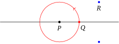
Figure 1. The (real) fibering of $\widetilde{F}$ in the case three-pointsd. The spaces $\mathbb{C}^{2}\setminus\{P\}\simeq S^{3}$ and $\mathbb{C}^{2}\setminus\left\langle P,Q\right\rangle\simeq S^{1}$ in the complex fiber respectively correspond to the pictured $S^{1}$ and $S^{0}$ in the real points.

three-pointse, $P,Q,R\notin\ell$, $P$, $Q$ and $\ell$ coplanar, but $R$ not on that plane:

Mapping $\{P,Q,R\}\mapsto\{P,Q\}$, we get a fiber bundle

and we are again done, similar to the case three-pointsb above.

three-pointsf, $P,Q,R\notin\ell$, no two coplanar with $\ell$:

In this case, we go to the $\mathfrak{S}_{3}$ cover $\widetilde{A}$ of $A$, so that similar to above, $H^{*}(A;\pm\mathbb{Q})$ is the sign-representation summand of $H^{*}(\widetilde{A};\mathbb{Q})$. Then $\widetilde{A}$ can be broken up by fiber bundles (see Fig. 2):

The $\mathfrak{S}_{3}$ action on $H^{*}(\widetilde{A})$ is again trivial by arguments similar to above.

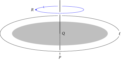
Figure 2. The (real) fiber for $R$ in the cover $\widetilde{A}$ of $A$. The complex fiber is homeomorphic to $(\mathbb{C}\setminus 0)\times(\mathbb{C}^{2}\setminus 0)$. The point $P$ and the line $\ell$ are at infinity, and the loop pictured corresponds to the generator in $H^{3}(\mathbb{C}^{2}\setminus 0)$.

four-pointsb, $P\in\ell$, $Q,R,S\notin\ell$, $Q$ and $R$ coplanar with $\ell$, $S$ not on that plane:

Similar to above, mapping $\{P,Q,R,S\}\mapsto\{Q,R,S\}$ we get a fiber bundle:

We are done by previous arguments.

four-pointsc, $P\in\ell$, $Q,R,S\notin\ell$, no two of $Q$, $R$ and $S$ coplanar with $\ell$:

Mapping $\{P,Q,R,S\}\mapsto\{Q,R,S\}$ we get a fiber bundle:

We are done by previous arguments.

four-pointsd, $P,Q,R,S\notin\ell$, $P$, $Q$, $R$ coplanar with $\ell$, $S$ not on that plane:

Mapping $\{P,Q,R,S\}\mapsto\{P,Q,R\}$:

We are done by previous arguments.

four-pointse, $P,Q,R,S\notin\ell$, $P$ and $Q$ coplanar with $\ell$, $R$ and $S$ coplanar with $\ell$:

We can map $\{P,Q,R,S\}\mapsto\{\left\langle P,Q\right\rangle,\left\langle R,S\right\rangle\}$, the two lines through $PQ$ and $RS$ and get a map $A\to B$, where $B$ is the set of unordered pairs of lines in $\mathbb{P}^{3}$ that both intersect $\ell$, but so that the three lines are not coplanar (in particular the pair of lines do not themselves intersect). This is a fiber bundle:

Since $L_{i}\setminus\ell\cong\mathbb{C}$, and $H^{*}(\operatorname{UConf}_{2}(\mathbb{C}),\pm\mathbb{Q})=0$, $H^{*}(A;\pm\mathbb{Q})=0$.

four-pointsf, $P,Q,R,S\notin\ell$, $P$ and $Q$ coplanar with $\ell$, no other pair coplanar with $\ell$:

Forthis case mapping $\{P,Q,R,S\}\mapsto\{P,Q\}$, we get a fiber bundle:

Here the local coefficients $\pm\mathbb{Q}$ on $A$ is induced by $\pm\mathbb{Q}$ on $A$ and $\pm\mathbb{Q}$ on the fibers $\{\{R,S\}\}\subset\operatorname{UConf}_{2}(\mathbb{P}^{3})$. We are done by previous arguments.

four-pointsg, $P,Q,R,S\notin\ell$, no two coplanar with $\ell$:

By an argument analogous to the case of three-pointsf, $A$ has an $\mathfrak{S}_{4}$ cover by ordering the four points that breaks up as a fiber bundle over the $\mathfrak{S}_{3}$ cover of $A$. The sign representation doesn’t occur in the cohomology of this cover, so we are done.

Alternatively, one can note that $\operatorname{UConf}_{4}(\mathbb{P}^{3}\setminus\ell)$ has the following stratification:

$$\operatorname{UConf}_{4}(\mathbb{P}^{3}\setminus\ell)=\{\text{four coplanar points in $\mathbb{P}^{3}\setminus\ell$}\}\sqcup A\sqcup A\sqcup A\sqcup A\,\text{.}$$

The first term can be further stratified into two sets:

$$\{\text{four coplanar points in $\mathbb{P}^{3}\setminus\ell$}\}=Y_{0}\sqcup Y_{1}\,\text{,}$$

where

$$Y_{0}=\{\text{four points in $H\setminus\ell$ for $H$ some plane in $\mathbb{P}^{3}$ containing $\ell$}\}\,\text{,}$$

and

$$Y_{1}=\{\text{four points in $H\setminus\ell$ for $H$ some plane in $\mathbb{P}^{3}$ \emph{not} containing $\ell$}\}\,\text{.}$$

In either case, mapping to the plane $H$ gives us two fiber bundles

      

Using Section 3.2 and previous arguments,

$$H^{*}(\operatorname{UConf}_{4}(\mathbb{P}^{3}\setminus\mathbb{P}^{1});\pm\mathbb{Q})\cong H^{*}(Y_{0};\pm\mathbb{Q})\cong H^{*}(Y_{1};\pm\mathbb{Q})=0\,\text{.}$$

Since we’ve already shown that $A$, $A$ and $A$ are $\pm\mathbb{Q}$-acyclic, $A$ must be as well.

∎

Recall that by (2) we have spectral sequences $E^{r}_{p,q}\implies\mkern 1.5mu\overline{\mkern-1.5muH\mkern-1.5mu}\mkern 1.5mu_{p+q}(\sigma)$ and $e^{r}_{p,q}$ that let us compute $\mkern 1.5mu\overline{\mkern-1.5muH\mkern-1.5mu}\mkern 1.5mu_{*}(F)=\widetilde{H}_{*-1}(Z)$, where

$$Z=\bigcup_{i\neq}\Phi_{i}\,\text{.}$$

Proposition 3.4.

The spectral sequence $E^{r}_{p,q}\implies\mkern 1.5mu\overline{\mkern-1.5muH\mkern-1.5mu}\mkern 1.5mu_{p+q}(\sigma)$ has the page $E^{1}_{p,q}$ as in Fig. 3. The spectral sequence $e^{r}_{p,q}\implies H_{p+q}(Z)$ has the page $e^{1}_{p,q}$ as in Fig. 4.

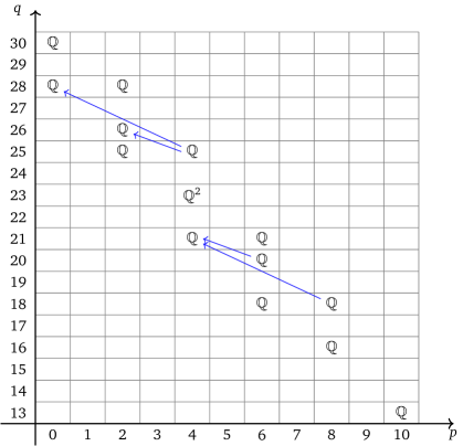
Figure 3. Spectral sequence page $E^{1}_{p,q}$ for $\mkern 1.5mu\overline{\mkern-1.5muH\mkern-1.5mu}\mkern 1.5mu_{p+q}(\sigma)$ (with $0$s omitted) and all potentially non-zero differentials in subsequent pages

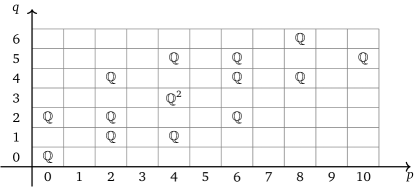
Figure 4. Spectral sequence page $e^{1}_{p,q}$ for $H_{p+q}(Z)$ (with $0$s omitted)

Proof.

Recall that by construction, the terms of $E^{1}$ and $e^{1}$ are related by Thom isomorphisms:

$$E^{1}_{p,q+2(14-p)}\cong e^{1}_{p,q}$$

except for $p=14$, where $e^{1}_{14,*}\equiv 0$. So we first go through more case work to establish columns $p\neq 14$.

By Eqs. 3.2, 3.3 and 3.4 and careful bookkeeping, it is enough to find $H^{*}(A_{i};\pm\mathbb{Q})$ along with the numbers $\dim(A_{i})=\dim_{\mathbb{C}}(A_{i})$ and $\dim(L(K))=\dim_{\mathbb{C}}(L(K))$ for $K\in A_{i}$, for the subtypes $i$ of I, II, IV VII (see Table 1 for the relevant numerics). Further, there are only eight subtypes remaining — the exceptions from Section 3.3.

$i$	pointa	pointb	two-pointsa	two-pointsb	two-pointsd	three-pointsa	three-pointsc	four-pointsa	XI
$\dim A_{i}$	$1$	$3$	$2$	$4$	$6$	$5$	$7$	$8$	$0$
$\dim L(K)$	$14$	$12$	$12$	$10$	$8$	$8$	$6$	$4$	$0$

Table 1. $\dim A_{i}$ and $\dim L(K)$ for $K\in A_{i}$ for each subtype $i$ excepted in Section 3.3.

pointa, $P\in\ell$:

$A=\ell\cong\mathbb{P}^{1}$, since there is only one point, the coefficients $\pm\mathbb{Q}$ are trivial, so

$$H^{*}(A;\pm\mathbb{Q})=H^{*}(\mathbb{P}^{1})=\begin{cases*}\mathbb{Q}&$*=0,2$\\ 0&otherwise.\end{cases*}$$

This contributes to $E^{1}_{0,28}\cong e^{1}_{0,0}$ and $E^{1}_{0,30}\cong e^{1}_{0,2}$ since $\dim(A)=1$ and $\dim(L(K))=14$.

pointb, $P\notin\ell$:

$A=\mathbb{P}^{3}-\ell\simeq\mathbb{P}^{1}$. Again, the coefficients are trivial, so

$$H^{*}(A;\pm\mathbb{Q})=H^{*}(\mathbb{P}^{1})=\begin{cases*}\mathbb{Q}&$*=0,2$\\ 0&otherwise.\end{cases*}$$

This contributes to $E^{1}_{2,26}\cong e^{1}_{2,2}$ and $E^{1}_{2,28}\cong e^{1}_{2,4}$ since $\dim(A)=3$ and $\dim(L(K))=12$.

two-pointsa, $P,Q\in\ell$:

$A=\operatorname{UConf}_{2}(\ell)\cong\operatorname{UConf}_{2}(\mathbb{P}^{1})$. By Section 3.2,

$$H^{*}(A;\pm\mathbb{Q})=\begin{cases*}\mathbb{Q}&$*=2$\\ 0&otherwise.\end{cases*}$$

This contributes to $E^{1}_{2,25}\cong e^{1}_{2,1}$ since $\dim(A)=2$ and $\dim(L(K))=12$.

two-pointsb, $P\in\ell$, $Q\notin\ell$:

$A\cong\ell\times(\mathbb{P}^{3}\setminus\ell)\simeq\mathbb{P}^{1}\times\mathbb{P}^{1}$ and the coefficients are trivial. Hence,

$$H^{*}(A;\pm\mathbb{Q})\cong H^{*}(\mathbb{P}^{1}\times\mathbb{P}^{1})=\begin{cases*}\mathbb{Q}&$*=0,4$\\ \mathbb{Q}^{2}&$*=2$\\ 0&otherwise.\end{cases*}$$

This contributes to $E^{1}_{4,21}\cong e^{1}_{4,1}$, $E^{1}_{4,23}\cong e^{1}_{4,3}$ and $E^{1}_{4,25}\cong e^{1}_{4,5}$ since $\dim(A)=4$ and $\dim(L(K))=10$.

two-pointsd, $P,Q\notin\ell$, $P$ and $Q$ not coplanar with $\ell$:

$A=\operatorname{UConf}_{2}(\mathbb{P}^{3}\setminus\ell)\setminus A)$. Section 3.3 shows that $H^{*}(A;\pm\mathbb{Q})=0$, so from the Gysin sequence, and by Section 3.2,

$$H^{*}(A,\pm\mathbb{Q})\cong H^{*}(\operatorname{UConf}_{2}(\mathbb{P}^{3}\setminus\mathbb{P}^{1}),\pm\mathbb{Q})=\begin{cases*}\mathbb{Q}&$*=0,2$\\ 0&otherwise.\end{cases*}$$

This contributes to $E^{1}_{6,21}\cong e^{1}_{6,5}$ since $\dim(A)=6$ and $\dim(L(K))=8$.

three-pointsa, $P,Q\in\ell$, $R\notin\ell$:

$A\cong\operatorname{UConf}_{2}(\ell)\times(\mathbb{P}^{3}\setminus\ell)$, and the local coefficients restrict to trivial coefficients on the second factor $\mathbb{P}^{3}\setminus\ell\simeq\mathbb{P}^{1}$. Thus,

$$H^{*}(A;\pm\mathbb{Q})\cong\oplus_{a+b=*}H^{a}(\operatorname{UConf}_{2}(\mathbb{P}^{1});\pm\mathbb{Q})\otimes H^{b}(\mathbb{P}^{1})=\begin{cases*}\mathbb{Q}&$*=2,4$\\ 0&otherwise.\end{cases*}$$

This contributes to $E^{1}_{6,18}\cong e^{1}_{6,2}$ and $E^{1}_{6,20}\cong e^{1}_{6,4}$ since $\dim(A)=5$ and $\dim(L(K))=8$.

three-pointsc, $P\in\ell$, $Q,R\notin\ell$, $Q$ and $R$ not coplanar with $\ell$:

Since the line $\left\langle Q,R\right\rangle$ doesn’t intersect $\ell$, $P$ can be any point on $\ell$ for any choice of $Q$ and $R$. Thus $A=\ell\times A$ and the local coefficients are trivial on the first factor ($\ell$ is anyway simply connected). Hence

$$H^{*}(A;\pm\mathbb{Q})\cong\oplus_{a+b=*}H^{a}(\mathbb{P}^{1})\otimes H^{b}(A;\pm\mathbb{Q})=\begin{cases*}\mathbb{Q}&$*=2,4$\\ 0&otherwise.\end{cases*}$$

This contributes to $E^{1}_{8,16}\cong e^{1}_{8,4}$ and $E^{1}_{8,18}\cong e^{1}_{8,6}$ since $\dim(A)=7$ and $\dim(L(K))=6$.

four-pointsa, $P,Q\in\ell$, $R,S\notin\ell$:

By definition of VII, the four points cannot be coplanar. This is equivalent to $R$ and $S$ not being coplanar with $\ell$. If $\rho\vcentcolon\mathbb{P}^{3}\setminus\ell\to\ell^{\perp}$ is the projection, then this is further equivalent to $\rho(R)\neq\rho(S)$. Note that $\rho^{-1}(T)=\left\langle T,\ell\right\rangle\setminus\ell\cong\mathbb{C}^{2}$. Thus, mapping $\{P,Q,R,S\}\mapsto(\{P,Q\},\{\rho(R),\rho(S)\})$, we get a bundle:

This implies, using Section 3.2,

$$H^{*}(A;\pm\mathbb{Q})\cong\oplus_{a+b=*}H^{a}(\operatorname{UConf}_{2}(\mathbb{P}^{1});\pm\mathbb{Q})\otimes H^{a}(\operatorname{UConf}_{2}(\mathbb{P}^{1});\pm\mathbb{Q})=\begin{cases*}\mathbb{Q}&$*=4$\\ 0&otherwise.\end{cases*}$$

This contributes to $E^{1}_{10,13}\cong e^{1}_{10,5}$ since $\dim(A)=8$ and $\dim(L(K))=4$.

Thus we’ve computed the pages $e^{1}_{p,q}$ and $E^{1}_{p,q}$ except the $p=14$ column of the latter. For XI, $L(K)=0$, so $E^{1}_{14,q}\cong\mkern 1.5mu\overline{\mkern-1.5muH\mkern-1.5mu}\mkern 1.5mu_{14+q}(\Phi)$. Now, if any term with $1\leq d=p+q\leq 14$ remains non-zero in $e^{\infty}_{p,q}$, then it would appear as $\mkern 1.5mu\overline{\mkern-1.5muH\mkern-1.5mu}\mkern 1.5mu_{d+1}(\Phi)$ and hence as a term $E^{1}_{14,d-13}$, which cannot interact with any of the other terms, by the shapes of the other columns, which we have already determined. That means $0\neq\mkern 1.5mu\overline{\mkern-1.5muH\mkern-1.5mu}\mkern 1.5mu_{d+1}(\sigma)\cong\widetilde{H}^{31-d}(\widetilde{X}_{\ell})$, which is a contradiction with $\widetilde{X}_{\ell}$ being a $16$-dimensional Stein manifold, as in Section 3.1. This implies, given the shape of $e^{1}_{p,q}$, that $\mkern 1.5mu\overline{\mkern-1.5muH\mkern-1.5mu}\mkern 1.5mu_{*}(\Phi)\equiv 0$, so we have also verified $E^{1}_{14,*}$. ∎

Proposition 3.4.

The spectral sequence $E^{r}_{p,q}$ degenerates at $r=1$ and hence the rational cohomology of $\widetilde{X}_{\ell}$ is given by

$$H^{*}(\widetilde{X}_{\ell};\mathbb{Q})\cong\begin{cases*}\mathbb{Q}&if $*=0,2,6,8$\\ \mathbb{Q}^{2}&if $*=1,3,5,7$\\ \mathbb{Q}^{4}&if $*=4$\\ 0&otherwise.\end{cases*}$$

Proof.

Recall that $E^{r}_{p,q}\implies\mkern 1.5mu\overline{\mkern-1.5muH\mkern-1.5mu}\mkern 1.5mu_{p+q}(\sigma)\cong\widetilde{H}^{31-p-q}(\sigma)$. The page $E^{1}_{p,q}$ is quite sparse to begin with, the only potentially non-zero differentials (on any page) are shown in Fig. 3. By Section 2.2, since $\widetilde{X}_{\ell}=\Pi_{l}\setminus\mathcal{V}(\Delta_{\ell})$, we must have

$$P_{\mathbb{Q}}(\widetilde{X}_{\ell},t)=P_{\mathbb{Q}}(\mathbb{C}^{\times},t)P_{\mathbb{Q}}(\widetilde{M}_{\ell},t)=(1+t)P_{\mathbb{Q}}(\widetilde{M}_{\ell},t)\,\text{,}$$

where $P_{\mathbb{Q}}(\_,t)$ denotes the (rational) Poincaré polynomial. This shows that $H^{2}(\widetilde{X}_{\ell})\cong\mkern 1.5mu\overline{\mkern-1.5muH\mkern-1.5mu}\mkern 1.5mu_{29}(\sigma)$ and $H^{6}(\widetilde{X}_{\ell})\cong\mkern 1.5mu\overline{\mkern-1.5muH\mkern-1.5mu}\mkern 1.5mu_{25}(\sigma)$ cannot be $0$, which means all those differentials must vanish. So $E^{\infty}_{p,q}\cong E^{1}_{p,q}$ and there are no extension problems with rational coefficients. ∎

References

- [ACT02] Daniel Allcock, James A. Carlson and Domingo Toledo “The complex hyperbolic geometry of the moduli space of cubic surfaces” In J. Algebraic Geom. 11.4 American Mathematical Society (AMS), 2002, pp. 659–724 DOI: 10.1090/S1056-3911-02-00314-4
- [Car85] R.. Carter “Finite groups of Lie type: conjugacy classes and irreducible characters” Wiley Classics Lib.(Wiley, Chichester, 1993), 1985
- [Cay49] Arthur Cayley “On the triple tangent planes of surfaces of the third order” In The Cambridge and Dublin mathematical journal 4, 1849, pp. 118–132
- [Del77] P. Deligne “Cohomologie étale” Séminaire de géométrie algébrique du Bois-Marie SGA 569, Lecture Notes in Mathematics Springer-Verlag, Berlin, 1977, pp. iv+312 DOI: 10.1007/BFb0091526
- [Del80] Pierre Deligne “La conjecture de Weil. II” In Inst. Hautes Études Sci. Publ. Math. Springer Nature, 1980, pp. 137–252 DOI: 10.1007/bf02684780
- [DvGK05] I. Dolgachev, B. Geemen and S. Kondō “A complex ball uniformization of the moduli space of cubic surfaces via periods of surfaces” In J. Reine Angew. Math. 588, 2005, pp. 99–148 DOI: 10.1515/crll.2005.2005.588.99
- [Gor05] Alexei G. Gorinov “Real cohomology groups of the space of nonsingular curves of degree 5 in ” In Ann. Fac. Sci. Toulouse Math. (6) 14.3, 2005, pp. 395–434 DOI: 10.1007/bf02684780
- [Har79] Joe Harris “Galois groups of enumerative problems” In Duke Math. J. 46.4 Duke University Press, 1979, pp. 685–724 DOI: 10.1215/s0012-7094-79-04635-0
- [Jor89] Camille Jordan “Traité des substitutions et des équations algébriques” Reprint of the 1870 original, Les Grands Classiques Gauthier-Villars. [Gauthier-Villars Great Classics] Éditions Jacques Gabay, Sceaux, 1989, pp. xvi+670
- [Loo08] Eduard Looijenga “Artin groups and the fundamental groups of some moduli spaces” In J. Topol. 1.1 Oxford University Press (OUP), 2008, pp. 187–216 DOI: 10.1112/jtopol/jtm009
- [Man86] Yu.. Manin “Cubic forms” Algebra, geometry, arithmetic, Translated from the Russian by M. Hazewinkel 4, North-Holland Mathematical Library North-Holland Publishing Co., Amsterdam, 1986, pp. x+326
- [Mil13] James S. Milne “Lectures on Etale Cohomology (v2.21)”, 2013, pp. 202 URL: www.jmilne.org/math/
- [Nar82] Isao Naruki “Cross ratio variety as a moduli space of cubic surfaces” With an appendix by Eduard Looijenga In Proc. London Math. Soc. (3) 45.1 Oxford University Press (OUP), 1982, pp. 1–30 DOI: 10.1112/plms/s3-45.1.1
- [PS03] C… Peters and J… Steenbrink “Degeneration of the Leray spectral sequence for certain geometric quotients” In Mosc. Math. J. 3.3, 2003, pp. 1085–1095\bibrangessep1201
- [Tom05] Orsola Tommasi “Rational cohomology of the moduli space of genus 4 curves” In Compos. Math. 141.2 Oxford University Press (OUP), 2005, pp. 359–384 DOI: 10.1112/s0010437x0400123x
- [Tom14] Orsola Tommasi “Stable cohomology of spaces of non-singular hypersurfaces” In Adv. Math. 265 Elsevier BV, 2014, pp. 428–440 DOI: 10.1016/j.aim.2014.08.005
- [Tot96] Burt Totaro “Configuration spaces of algebraic varieties” In Topology 35.4, 1996, pp. 1057–1067 DOI: 10.1016/0040-9383(95)00058-5
- [Vas99] Victor Anatolievich Vasil’ev “How to calculate the homology of spaces of nonsingular algebraic projective hypersurfaces” In Tr. Mat. Inst. Steklova 225.Solitony Geom. Topol. na Perekrest., 1999, pp. 132–152