Nonlinear stability at the Eckhaus boundary

Abstract

The real Ginzburg-Landau equation possesses a family of spatially periodic equilibria. If the wave number of an equilibrium is strictly below the so called Eckhaus boundary the equilibrium is known to be spectrally and diffusively stable, i.e., stable w.r.t. small spatially localized perturbations. If the wave number is above the Eckhaus boundary the equilibrium is unstable. Exactly at the boundary spectral stability holds. The purpose of the present paper is to establish the diffusive stability of these equilibria. The limit profile is determined by a nonlinear equation since a nonlinear term turns out to be marginal w.r.t. the linearized dynamics.

1 Introduction

The Ginzburg-Landau equation

$$\partial_{T}A=\partial^{2}_{X}A+A-A\left|A\right|^{2},$$ (1)

with $T\geq 0$, $X\in\mathbb{R}$, and $A(X,T)\in\mathbb{C}$ appears as a universal amplitude equation for the description of a number of pattern forming systems close to the first instability, cf. [NW69]. See [SZ13, SU17] for a recent overview about the mathematical justification of the so called Ginzburg-Landau approximation. The stationary solutions of (1), namely

$$A_{q}=\sqrt{1-q^{2}}e^{iqX}$$ (2)

are known to be spectrally stable for $q^{2}\leq 1/3$ and unstable for $q^{2}>1/3$. This was observed first in [Eck65] and therefore $q^{2}=1/3$ is called the Eckhaus or sideband stability boundary.

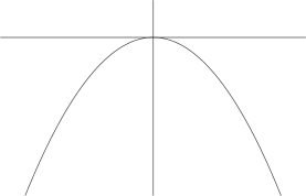
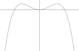
Figure 1: The linearization around the equilibrium is solved by $e^{ikx+\lambda_{1,2}t}V_{1,2}$ with $V_{1,2}\in\mathbb{C}^{2}$ and $\lambda_{1}(k)>\lambda_{2}(k)$. The left panel shows the curve $k\mapsto\lambda_{1}(k)$ in the stable case and the right panel in the unstable case.

It took more than twenty years to establish the diffusive stability of the spectrally stable equilibria, i.e., the stability w.r.t. small spatially localized perturbations. In [CEE92] this result has been shown by using $L^{1}$-$L^{\infty}$ estimates and in [BK92] by using a renormalization group approach to additionally establish the exact asymptotic decay of the perturbation in time. The proofs are based on the fact that the nonlinear terms are irrelevant w.r.t. the linear diffusion

$$\varphi(X,T)=\frac{\varphi^{*}}{\sqrt{T}}e^{-\frac{X^{2}}{4T}}+\mathcal{O}\!\left(\frac{1}{T}\right),$$

and so the renormalized perturbation converges towards a Gaussian limit.

In contrast to exponential decay rates, polynomial decay rates occurring in diffusion do not allow in general to control all nonlinear terms in a neighborhood of the origin. The nonlinear terms can be divided into irrelevant ones which show faster decay rates than the linear diffusion terms $\partial_{T}\varphi$ and $\partial_{X}^{2}\varphi$, into marginal ones which show the same decay rates and into the ones which decay slower and which would lead to a completely different asymptotic behavior for $T\to\infty$. Linear diffusive behavior exhibits the following asymptotic decay rates

$$\varphi\sim T^{-1/2},\quad\partial_{X}\sim T^{-1/2},\quad\text{and}\quad\partial_{T}\sim T^{-1}$$

and so in a nonlinear diffusion equation

$$\partial_{T}\varphi-\partial_{X}^{2}\varphi=\varphi^{p_{0}}(\partial_{X}\varphi)^{p_{1}}(\partial_{X}^{2}\varphi)^{p_{2}}$$

the terms on the left hand side both exhibit a decay rate $T^{-3/2}$, whereas the right hand side decays as $T^{-(p_{0}+2p_{1}+3p_{2})/2}$. More precisely, a term $\varphi^{2}$ cannot be controlled by diffusion, a term $-\varphi^{3}$ leads to a faster decay, a term $+\varphi^{3}$ to a logarithmic growth, and a Burgers term $\varphi\partial_{X}\varphi$ is not changing the decay rates, but the limit profile from a Gaussian into a perturbed Gaussian. All other terms, satisfying $p_{0}+2p_{1}+3p_{2}\geq 4$, can be controlled asymptotically by the left hand side. In order to prove that a smooth nonlinearity $H=H(\varphi,\partial_{X}\varphi,\partial_{X}^{2}\varphi)$ can be controlled by diffusion we have to show that the coefficients in front of $\varphi^{2}$ and $\varphi^{3}$ vanish. This idea has been generalized to very general systems where $\partial_{X}^{2}$ has been replaced by operators which possess a curve of eigenvalues with a parabolic profile for $k\to 0$ in Fourier or Bloch space. In many such systems the nonlinear terms turn out be irrelevant [Sch98, DSSS09, SSSU12, JNRZ14].

Exactly at the Eckhaus stability boundary, $q^{2}=1/3$, spectral stability still holds, but only with $\lambda_{1}\sim-k^{4}$ instead of $\lambda_{1}\sim-k^{2}$ for $k\to 0$ as shown in Figure 1. Therefore, we only have the much slower asymptotic decay rates

$$\varphi\sim T^{-1/4},\quad\partial_{X}\sim T^{-1/4},\quad\text{and}\quad\partial_{T}\sim T^{-1}.$$

Due to this slow decay there is a nonlinear term which is marginal w.r.t. the linear dynamics. We find an effective equation of the form

$$\partial_{T}\varphi+\nu_{1}\partial^{4}_{X}\varphi=\nu_{2}\partial_{X}\left((\partial_{X}\varphi)^{2}\right)+g_{1},$$ (3)

with coefficients $\nu_{1}>0$ and $\nu_{2}<0$. The first term on the right hand side decays as $\sim T^{-5/4}$ like the linear ones on the left hand side. In $g_{1}$ we collect all terms with faster decay rates. Fortunately, it turns out that $\nu_{2}\partial_{X}\left((\partial_{X}\varphi)^{2}\right)$ is not changing the decay rates, but only leads to a nonlinear correction of the limit profile like the Burgers term $\varphi\partial_{X}\varphi$ for diffusion [BKL94]. Our result is therefore as follows.

Theorem 1.1.

For all $C>0$, there exists $\delta>0$ such that for any $\widehat{V}_{0}\in L^{1}\cap L^{\infty}$ satisfying $\|\widehat{V}_{0}\|_{L^{1}}+\|\widehat{V}_{0}\|_{L^{\infty}}\leq\delta$, the solution $A=A_{\sqrt{1/3}}+V$ of the Ginzburg-Landau equation (1) with $V|_{T=0}=V_{0}$ satisfies

$$\|\widehat{V}(T)\|_{L^{\infty}}\leq C\qquad\text{and}\qquad\|V(T)\|_{L^{\infty}}\leq\|\widehat{V}(T)\|_{L^{1}}\leq C(1{+}T)^{-\frac{1}{4}}$$

for all $T\geq 0$.

The proof is an adaption of the $L^{1}$-$L^{\infty}$ scheme presented in [MSU01] to the situation of a coupling of linearly diffusive modes with linearly exponentially damped modes. The complications are due to the marginal relevant nonlinear term and the slower decay rates. We strongly believe that our result can be transferred to general pattern forming systems, too.

The plan of the paper is as follows. Section 2 recalls the formal calculations to derive (3). This section is not necessary for the proof of Theorem 1.1 but helps to understand the subsequent steps of the proof. The proof of Theorem 1.1 starts in Section 3 with the separation of the linearly diffusive and the linearly exponentially damped modes in a suitably chosen coordinate system. In Section 3.2 we establish the linear decay estimates. The formal irrelevance of the nonlinear terms can be found in Section 3.3 and in Appendix B. The final nonlinear decay estimates can be found in Section 4. For completeness the limit profile of the renormalized solution is computed in Appendix A.

For some of the following explicit calculations the software Mathematica [Wol] was used.

Notation. We define the Fourier transform by

$$\widehat{u}(k)=(\mathcal{F}u)(k)=\frac{1}{2\pi}\int_{{\mathbb{R}}}u(x)e^{-ikx}\mathrm{d}x$$

and the inverse Fourier transform by

$$u(x)=(\mathcal{F}^{-1}\widehat{u})(x)=\int_{{\mathbb{R}}}\widehat{u}(k)e^{ikx}\mathrm{d}k.$$

We have $\|u\|_{\infty}\leq\|\widehat{u}\|_{1}$, where $\|u\|_{\infty}=\sup_{x\in{\mathbb{R}}}|u(x)|$ is the norm in the space of bounded uniformly continuous functions and $\|u\|_{1}=\int_{{\mathbb{R}}}|u(x)|\mathrm{d}x$ the norm in the Lebesgue space $L^{1}$.

2 Some formal calculations

In this section we formally derive (3). This section is not necessary for the proof of Theorem 1.1 but helps to understand the subsequent steps of the proof.

2.1 Equations for the deviation

In order to obtain a semilinear system with $X$-independent coefficients we introduce the deviation $V$ from $A_{q}$ not in an additive, but in a multiplicative way, i.e., we set

$$A(X,T)=A_{\sqrt{1/3}}(X)(1+V(X,T))=\sqrt{\textstyle\frac{2}{3}}e^{i\sqrt{1/3}X}(1+V(X,T)).$$ (4)

With

$$\partial_{X}A =A_{\sqrt{1/3}}\partial_{X}V+i\sqrt{\tfrac{1}{3}}A_{\sqrt{1/3}}+i\sqrt{\tfrac{1}{3}}A_{\sqrt{1/3}}V,$$

$$\partial_{X}^{2}A =A_{\sqrt{1/3}}\partial_{X}^{2}V+2i\sqrt{\tfrac{1}{3}}\partial_{X}V-\tfrac{1}{3}A_{\sqrt{1/3}}-\tfrac{1}{3}A_{\sqrt{1/3}}V$$

we find

$$\partial_{T}V=\partial_{X}^{2}V+2i\sqrt{\tfrac{1}{3}}\partial_{X}V-\tfrac{2}{3}V-\tfrac{2}{3}\overline{V}-\tfrac{2}{3}V^{2}-\tfrac{4}{3}|V|^{2}-\tfrac{2}{3}V|V|^{2}.$$

Now we split the above equation into real and imaginary part. We introduce $V_{r}=\mathrm{Re}\,V$, $V_{i}=\mathrm{Im}\,V$ and obtain

$$\begin{array}[]{rcl}\partial_{T}V_{r}&=&\partial_{X}^{2}V_{r}-\tfrac{4}{3}V_{r}-2\sqrt{\tfrac{1}{3}}\partial_{X}V_{i}-\frac{2}{3}(3V_{r}^{2}+V_{i}^{2}+V_{r}^{3}+V_{r}V_{i}^{2}),\\ \partial_{T}V_{i}&=&\partial_{X}^{2}V_{i}+2\sqrt{\tfrac{1}{3}}\partial_{X}V_{r}-\frac{2}{3}(2V_{r}V_{i}+V_{r}^{2}V_{i}+V_{i}^{3}).\end{array}$$ (5)

2.2 Spectral analysis

The linearization around $(V_{r},V_{i})=(0,0)$ is given by

$$\partial_{T}V_{r} =\partial^{2}_{X}V_{r}-\frac{4}{3}V_{r}-2\sqrt{\tfrac{1}{3}}\partial_{X}V_{i},$$

$$\partial_{T}V_{i} =\partial^{2}_{X}V_{i}+2\sqrt{\tfrac{1}{3}}\partial_{X}V_{r}.$$

It is solved by

$$V_{r}=\widehat{V}_{r}e^{ikX}e^{\lambda T},\quad V_{i}=\widehat{V}_{i}e^{ikX}e^{\lambda T},$$

where

$$\lambda\widehat{V}_{r} =-k^{2}\widehat{V}_{r}-\frac{4}{3}\widehat{V}_{r}-2\sqrt{\tfrac{1}{3}}ik\widehat{V}_{i},$$

$$\lambda\widehat{V}_{i} =-k^{2}\widehat{V}_{i}+2\sqrt{\tfrac{1}{3}}ik\widehat{V}_{r}.$$

The condition for non-trivial solutions

$$\det\begin{pmatrix}-k^{2}-\lambda-\frac{4}{3}&-2\sqrt{\tfrac{1}{3}}ik\\ 2\sqrt{\tfrac{1}{3}}ik&-k^{2}-\lambda\end{pmatrix}=\lambda^{2}+2k^{2}\lambda+k^{4}+\frac{4}{3}\lambda=0$$

leads to the curves of eigenvalues

$$2\lambda_{1/2}(k)=-\left(2k^{2}+\frac{4}{3}\right)\pm\sqrt{\left(2k^{2}+\frac{4}{3}\right)^{2}-4k^{4}}.$$ (6)

The expansion at $k=0$ is given by

$$\lambda_{1}(k)=-\frac{3}{4}k^{4}+\mathcal{O}(k^{6}),\quad\lambda_{2}(k)=-\frac{4}{3}+\mathcal{O}(k^{2}).$$

2.3 Linear asymptotic analysis

Hence, the modes associated to the curve $\lambda_{2}$ are exponentially damped, whereas the curve $\lambda_{1}$ comes up to zero and leads to at most to polynomial decay rates. For the linear equation the modes will concentrate at $k=0$ such that the expansion of $\lambda_{1}$ at $k=0$ plays a crucial role. Diagonalizing the linear part leads to a change of variables $(V_{r},V_{i})\mapsto(V_{s},V_{c})$ with the asymptotic model

$$\partial_{T}\widehat{V}_{c}=-\frac{3}{4}k^{4}\widehat{V}_{c}.$$

It is solved by

$$\widehat{V}_{c}(k,T)=e^{-\frac{3}{4}k^{4}T}\widehat{V}_{c}(k,0)$$

and shows some self-similar behavior, namely

$$\widehat{V}_{c}(\kappa T^{-\frac{1}{4}},T)=e^{-\frac{3}{4}\kappa^{4}}\widehat{V}_{c}(\kappa T^{-\frac{1}{4}},0)=e^{-\frac{3}{4}\kappa^{4}}(1+\mathcal{O}(T^{-1/4})),$$

provided the solution is normalized with $\widehat{V}_{c}(0,0)=1$. Hence, for $T\to\infty$ the solutions will behave like the self-similar solution

$$\widehat{V}_{c}(k,T)=\widehat{\Phi}_{lin}\bigl{(}kT^{\frac{1}{4}}\bigr{)},\qquad\text{with}\qquad\widehat{\Phi}_{lin}(\kappa)=e^{-\frac{3}{4}\kappa^{4}}.$$

Transferring these formulas into physical space shows that for $T\to\infty$ the solutions of

$$\partial_{T}V_{c}=-\frac{3}{4}\partial^{4}_{X}V_{c}$$ (7)

will behave like the self-similar solution

$$V_{c}(X,T)={T^{-1/4}}{\Phi}_{lin}\bigl{(}{X}{T^{-1/4}}\bigr{)},$$ (8)

where ${\Phi}_{lin}=\mathcal{F}^{-1}\widehat{\Phi}_{lin}$.

At leading order in the limit $k\to 0$, we have

$$\widehat{V}_{r}=\widehat{V}_{s}-\tfrac{\sqrt{3}}{2}ik\widehat{V}_{c}\qquad\text{and}\qquad\widehat{V}_{i}=\widehat{V}_{c}-\tfrac{\sqrt{3}}{2}ik\widehat{V}_{s},$$

so we expect the following scaling in the original variables

$$V_{r}\sim{T^{-1/2}},\quad V_{i}\sim{T^{-1/4}},\quad\partial_{X}\sim{T^{-1/4}},\quad\text{and}\quad\partial_{T}\sim T^{-1},$$ (9)

at least at the linear level.

2.4 Nonlinear asymptotic analysis

According to the explanations from the introduction, polynomial decay rates do not allow to control all nonlinear terms in a neighborhood of the origin. Therefore, we have to compute the effective nonlinearity. As already said, it turns out that there is one marginal nonlinear term which leads to a nonlinear correction of the linear limit profile $\Phi_{lin}$, but not to an instability or to a change in the decay rates.

In order to compute this nonlinear correction to (7) we suppose that the dynamics is in fact controlled by the linear dynamics (8), i.e., we consider the asymptotic decays given by (9). Since $V_{c}$ is linearly exponentially damped at $k=0$, we expect that $V_{r}$ is slaved by $V_{i}$ for large times. We find

$$\underbrace{\partial_{T}V_{r}}_{\sim T^{-3/2}}=\underbrace{\partial_{X}^{2}V_{r}}_{\sim T^{-1}}-\underbrace{\tfrac{4}{3}V_{r}}_{\sim T^{-1/2}}-\underbrace{2\sqrt{\tfrac{1}{3}}\partial_{X}V_{i}}_{\sim T^{-1/2}}-\frac{2}{3}(\underbrace{3V_{r}^{2}}_{\sim T^{-1}}+\underbrace{V_{i}^{2}}_{\sim T^{-1/2}}+\underbrace{V_{r}^{3}}_{\sim T^{-3/2}}+\underbrace{V_{r}V_{i}^{2}}_{\sim T^{-1}}).$$

Equating the terms of decay $T^{-1/2}$ to zero yields

$$0=-\tfrac{4}{3}V_{r}-2\sqrt{\tfrac{1}{3}}\partial_{X}V_{i}-\tfrac{2}{3}V_{i}^{2}\qquad\text{or equivalently}\qquad V_{r}=-\tfrac{1}{2}\sqrt{3}\partial_{X}V_{i}-\tfrac{1}{2}V_{i}^{2}.$$

Inserting this into the equation for $V_{i}$

$$\underbrace{\partial_{T}V_{i}}_{\sim T^{-5/4}}=\underbrace{\partial_{X}^{2}V_{i}}_{\sim T^{-3/4}}+\underbrace{2\sqrt{\tfrac{1}{3}}\partial_{X}V_{r}}_{\sim T^{-3/4}}-\tfrac{2}{3}(\underbrace{2V_{r}V_{i}}_{\sim T^{-3/4}}+\underbrace{V_{r}^{2}V_{i}}_{\sim T^{-5/4}}+\underbrace{V_{i}^{3}}_{\sim T^{-3/4}})$$

gives for the terms of decay $T^{-3/4}$ that

$$\partial_{X}^{2}V_{i}+2\sqrt{\tfrac{1}{3}}\partial_{X}(-\tfrac{1}{2}\sqrt{3}\partial_{X}V_{i}-\tfrac{1}{2}V_{i}^{2})-\tfrac{4}{3}(-\tfrac{1}{2}\sqrt{3}\partial_{X}V_{i}-\tfrac{1}{2}V_{i}^{2})V_{i}-\tfrac{2}{3}V_{i}^{3}=0.$$

Since this expression vanishes identically, we need to include the $T^{-1}$ terms into the expression of $V_{r}$ in terms of $V_{i}$

$$\underbrace{\tfrac{4}{3}V_{r}}_{\sim T^{-1/2}} = \underbrace{\partial_{X}^{2}V_{r}}_{\sim T^{-1}}-\underbrace{2\sqrt{\tfrac{1}{3}}\partial_{X}V_{i}}_{\sim T^{-1/2}}-\tfrac{2}{3}(\underbrace{3V_{r}^{2}}_{\sim T^{-1}}+\underbrace{V_{i}^{2}}_{\sim T^{-1/2}}+\underbrace{V_{r}V_{i}^{2}}_{\sim T^{-1}})$$

$$= \underbrace{-2\sqrt{\tfrac{1}{3}}\partial_{X}V_{i}-\tfrac{2}{3}V_{i}^{2}}_{\sim T^{-1/2}}$$

$$+\tfrac{1}{6}(\underbrace{-V_{i}^{4}-15(\partial_{X}V_{i})^{2}-4\sqrt{3}V_{i}^{2}\partial_{X}V_{i}-6V_{i}\partial_{X}^{2}V_{i}-3\sqrt{3}\partial_{X}^{3}V_{i}}_{\sim T^{-1}}).$$

Inserting this into the equation for $V_{i}$ yields

$$\partial_{T}V_{i}=-\frac{3}{4}\partial^{4}_{X}V_{i}-\frac{3}{2}\sqrt{3}\partial_{X}\left((\partial_{X}V_{i})^{2}\right)+\mathcal{O}(T^{-5/4}).$$

Hence, there is a nonlinear term which is asymptotically of the same order as the linear terms $\partial_{T}V_{i}$ and $-\frac{3}{4}\partial_{X}^{4}V_{i}$ for $T\to\infty$ and so the asymptotic behavior will be governed by the self-similar solutions of

$$\partial_{T}V_{i}=-\frac{3}{4}\partial^{4}_{X}V_{i}-\frac{3}{2}\sqrt{3}\partial_{X}\left((\partial_{X}V_{i})^{2}\right).$$ (10)

Fortunately, as already said, the marginal term $-\frac{3}{2}\sqrt{3}\partial_{X}\left((\partial_{X}V_{i})^{2}\right)$ will only lead to a nonlinear correction of the limit profile, but not to an instability or to a change in the decay rates. Although not necessary for the proof of Theorem 1.1, the nonlinear correction of the limit profile is computed in Appendix A.

Remark 2.1.

It is not a surprise that a system of the form (10) is obtained. The so-called phase diffusion equations can be derived from the Ginzburg-Landau equation for the local wave number $\Psi$, cf. [MS04]. The amplitude $\Psi$ satisfies a system of the form $\partial_{\tau}\Psi=\partial_{\xi}^{2}h(\Psi)$ with $h^{\prime\prime}(0)=\lambda_{1}|_{k=0}[q]/2$, and describes small modulations in time $\tau=\delta T$ and space $\xi=\delta X$ of the periodic wave $A_{q}$, where $0<\delta\ll 1$ is a small perturbation parameter. This equation degenerates for $q^{2}=1/3$. Since at lowest order $\Psi\sim\partial_{\xi}V_{i}$, at $q^{2}=1/3$ we have a system

$$\partial_{\tau}V_{i}=\partial_{\xi}(h(\partial_{\xi}V_{i}))+h.o.t.\sim\partial_{\xi}((\partial_{\xi}V_{i})^{2})+h.o.t.$$

The linear term $\partial_{\xi}^{4}V_{i}$ is of higher order w.r.t. the scaling used in the derivation of the phase diffusion equation.

3 Some preparations

We start now with the proof of Theorem 1.1.

3.1 Separation of the diffusive modes

We introduce $v=(V_{r},V_{i})^{\top}$ and abbreviate (5) as

$$\partial_{T}v=Lv+N(v),$$

where

$$L=\begin{pmatrix}\partial_{X}^{2}-\tfrac{4}{3}&-2\sqrt{\tfrac{1}{3}}\partial_{X}\\ 2\sqrt{\tfrac{1}{3}}\partial_{X}&\partial_{X}^{2}\end{pmatrix}\qquad\text{and}\qquad N(v)=-\frac{2}{3}\begin{pmatrix}3V_{r}^{2}+V_{i}^{2}+V_{r}^{3}+V_{r}V_{i}^{2}\\ 2V_{r}V_{i}+V_{r}^{2}V_{i}+V_{i}^{3}\end{pmatrix}.$$

At this point it turns out to be advantageous to work in Fourier space. Hence we consider

$$\partial_{T}\widehat{v}=\widehat{L}\widehat{v}+\widehat{N}(\widehat{v}),$$ (11)

where $\widehat{v}=\mathcal{F}v$, $\widehat{L}=\mathcal{F}L\mathcal{F}^{-1}$, and $\widehat{N}(\widehat{v})=\mathcal{F}(N(\mathcal{F}^{-1}\widehat{v}))$.

There exists a $k_{0}>0$ such that for all $|k|\leq k_{0}$ the two curves of eigenvalues $\lambda_{1,2}$ defined in (6) are separated, and so we define

$$\widehat{P}_{c}(k)\widehat{v}(k)=\chi(k)\langle\widehat{\varphi}^{*}_{1}(k),\widehat{v}(k)\rangle\widehat{\varphi}_{1}(k),$$

where $\chi(k)=1$ for $|k|\leq k_{0}/2$, and $\chi(k)=0$ for $|k|>k_{0}/2$, and where $\widehat{\varphi}^{*}_{1}(k)$ is the eigenvector associated to the adjoint eigenvalue problem normalized by $\langle\widehat{\varphi}^{*}_{1}(k),\widehat{\varphi}_{1}(k)\rangle=1$. Moreover, define $\widehat{P}_{s}(k)\widehat{v}(k)=\widehat{v}(k)-\widehat{P}_{c}(k)\widehat{v}(k)$. We use the projections to separate (11) in two parts, namely

$$\partial_{T}\widehat{v}_{c}=\widehat{L}_{c}\widehat{v}_{c}+\widehat{P}_{c}\widehat{N}(\widehat{v}),\qquad\partial_{T}\widehat{v}_{s}=\widehat{L}_{s}\widehat{v}_{s}+\widehat{P}_{s}\widehat{N}(\widehat{v}),$$ (12)

where $\widehat{L}_{c}=\widehat{L}\widehat{P}_{c}$ and $\widehat{L}_{s}=\widehat{L}\widehat{P}_{s}$. By construction the operators $\widehat{P}_{s}$ and $\widehat{P}_{c}$ commute with $\widehat{L}$. System (12) is solved with $\widehat{v}_{c}|_{t=0}=\widehat{P}_{c}(k)\widehat{v}|_{t=0}$ and $\widehat{v}_{s}|_{t=0}=\widehat{P}_{s}(k)\widehat{v}|_{t=0}$. Then $\widehat{v}_{c}$ and $\widehat{v}_{s}$ are defined via the solutions of (12).

Moreover, we introduce $\widehat{V}_{c}$ by $\widehat{v}_{c}(k,t)=\widehat{V}_{c}(k,t)\widehat{\varphi}_{1}(k)$, and $\widehat{V}_{s}$ for $|k|\leq k_{0}/2$ by $\widehat{v}_{s}(k,t)=\widehat{V}_{s}(k,t)\widehat{\varphi}_{2}(k)$.

3.2 Linear decay estimates

In order to show the nonlinear stability of $A_{\sqrt{1/3}}$ we use the polyomial decay rates of the linear semigroup generated by $L$. However, the optimal decay rate $T^{-1/4}$ of the semigroup is only obtained as a mapping from $L^{1}$ to $L^{\infty}$ in physical space, or from $L^{\infty}$ to $L^{1}$ in Fourier space. Therefore, we have to work with at least two spaces. In Fourier space the $L^{\infty}$-norm of the solutions of $\partial_{T}\widehat{v}=\widehat{L}\widehat{v}$ will be bounded and the $L^{1}$-norm will decay as $T^{-1/4}$, both for initial conditions in $L^{\infty}\cap L^{1}$.

Since the sectorial operator $\widehat{L}_{s}$ has spectrum in the left half plane strictly bounded away from the imaginary axis, we obviously have the following result, cf. [Hen81].

Lemma 3.1.

For the analytic semigroup generated by $\widehat{L}_{s}$ we have the estimates

$$\|e^{T\widehat{L}_{s}}\|_{L^{1}\to L^{1}}\leq Ce^{-\sigma_{s}T/2},\quad\text{ and }\quad\|e^{T\widehat{L}_{s}}\|_{L^{\infty}\to L^{\infty}}\leq Ce^{-\sigma_{s}T/2},$$

with some $\sigma_{s}>0$.

For the $\widehat{v}_{c}$-part we obtain

Lemma 3.2.

Let $\nu\geq 0$. For the analytic semigroup generated by $\widehat{L}_{c}$ we have the estimates

$$\|e^{T\widehat{L}_{c}}|k|^{\nu}\|_{L^{1}\to L^{1}}\leq CT^{-\nu/4},\quad\|e^{T\widehat{L}_{c}}|k|^{\nu}\|_{L^{\infty}\to L^{\infty}}\leq CT^{-\nu/4},\quad\|e^{T\widehat{L}_{c}}|k|^{\nu}\|_{L^{\infty}\to L^{1}}\leq CT^{-(\nu+1)/4}.$$

Proof. Since $\lambda_{1}(k)\leq-Ck^{4}$ for small $k$ and $e^{T\widehat{L}_{c}(k)}\widehat{v}_{c}(k)=e^{\lambda_{1}(k)T}\widehat{v}_{c}(k)$ we obviously have

$$\|e^{T\widehat{L}_{c}}|k|^{\nu}\widehat{v}_{c}\|_{L^{1}} \leq \|e^{\lambda_{1}(k)T}|k|^{\nu}\|_{L^{\infty}}\|\widehat{v}_{c}\|_{L^{1}}\leq CT^{-\nu/4}\|\widehat{v}_{c}\|_{L^{1}},$$

$$\|e^{T\widehat{L}_{c}}|k|^{\nu}\widehat{v}_{c}\|_{L^{\infty}} \leq \|e^{\lambda_{1}(k)T}|k|^{\nu}\|_{L^{\infty}}\|\widehat{v}_{c}\|_{L^{\infty}}\leq CT^{-\nu/4}\|\widehat{v}_{c}\|_{L^{\infty}},$$

$$\|e^{T\widehat{L}_{c}}|k|^{\nu}\widehat{v}_{c}\|_{L^{1}} \leq \|e^{\lambda_{1}(k)T}|k|^{\nu}\|_{L^{1}}\|\widehat{v}_{c}\|_{L^{\infty}}\leq CT^{-(\nu+1)/4}\|\widehat{v}_{c}\|_{L^{\infty}}.$$

∎

3.3 Formal irrelevance of the nonlinear terms

After showing decay rates for the linear semigroup we have to establish the irrelevance of the nonlinearity w.r.t. this linear behavior. In view of future applications we will consider a general nonlinearity and not only quadratic and cubic terms. In order to do so we expand the nonlinear terms into

$$\widehat{P}_{c}\widehat{N}(\widehat{v}) = B_{2,1}(\widehat{v}_{c},\widehat{v}_{c})+B_{3,1}(\widehat{v}_{c},\widehat{v}_{c},\widehat{v}_{c})+B_{4,1}(\widehat{v}_{c},\widehat{v}_{c},\widehat{v}_{c},\widehat{v}_{c})+B_{5,1}(\widehat{v}_{c},\widehat{v}_{c},\widehat{v}_{c},\widehat{v}_{c},\widehat{v}_{c})$$

$$+B_{2,2}(\widehat{v}_{c},\widehat{v}_{s})+B_{3,2}(\widehat{v}_{c},\widehat{v}_{c},\widehat{v}_{s})+B_{4,2}(\widehat{v}_{c},\widehat{v}_{c},\widehat{v}_{c},\widehat{v}_{s})$$

$$+B_{2,3}(\widehat{v}_{s},\widehat{v}_{s})+B_{3,3}(\widehat{v}_{c},\widehat{v}_{s},\widehat{v}_{s})+g_{c}(\widehat{v}_{c},\widehat{v}_{s}),$$

$$\widehat{P}_{s}\widehat{N}(\widehat{v}) = B_{2,4}(\widehat{v}_{c},\widehat{v}_{c})+B_{3,4}(\widehat{v}_{c},\widehat{v}_{c},\widehat{v}_{c})+B_{4,4}(\widehat{v}_{c},\widehat{v}_{c},\widehat{v}_{c},\widehat{v}_{c})$$

$$+B_{2,5}(\widehat{v}_{c},\widehat{v}_{s})+B_{3,5}(\widehat{v}_{c},\widehat{v}_{c},\widehat{v}_{s})+B_{2,6}(\widehat{v}_{s},\widehat{v}_{s})+g_{s}(\widehat{v}_{c},\widehat{v}_{s}),$$

where the $B_{m,j}$ are symmetric $m$-linear mappings, and where $g_{c}$ and $g_{s}$ stand for the remaining terms, which due to Young’s inequality for convolutions satisfy

$$\|g_{c}(\widehat{v}_{c},\widehat{v}_{s})\|_{L^{1}} \leq C(\|\widehat{v}_{c}\|_{L^{1}}^{6}+\|\widehat{v}_{c}\|_{L^{1}}^{4}\|\widehat{v}_{s}\|_{L^{1}}+\|\widehat{v}_{c}\|_{L^{1}}^{2}\|\widehat{v}_{s}\|_{L^{1}}^{2}+\|\widehat{v}_{s}\|_{L^{1}}^{3}),$$

$$\|g_{s}(\widehat{v}_{c},\widehat{v}_{s})\|_{L^{1}} \leq C(\|\widehat{v}_{c}\|_{L^{1}}^{5}+\|\widehat{v}_{c}\|_{L^{1}}^{3}\|\widehat{v}_{s}\|_{L^{1}}+\|\widehat{v}_{c}\|_{L^{1}}\|\widehat{v}_{s}\|_{L^{1}}^{2}+\|\widehat{v}_{s}\|_{L^{1}}^{3})$$

for sufficiently small $\|\widehat{v}_{s}\|_{L^{1}}$ and $\|\widehat{v}_{s}\|_{L^{1}}$. We note that for the Ginzburg-Landau equation (11), the bilinear and trilinear terms are the only nonvanishing terms in these expansions. The splitting is motivated as follows. If $\widehat{v}_{c}$ decays like $T^{-1/4}$, then $\widehat{v}_{s}$, which is expected to be formally slaved to $\widehat{v}_{c}$, decays at least like $T^{-1/2}$. Then $g_{c}$ decays like $T^{-3/2}$ and is therefore irrelevant w.r.t. the linear dynamics of $\widehat{v}_{c}$. Here and in the following the decays are referred to the decay of the $L^{\infty}$-norm of $v$ or the $L^{1}$-norm of $\hat{v}$, cf. Section 4.

In order to prove the irrelevance of the other terms w.r.t. the linear dynamics of $\widehat{v}_{c}$, except for the marginal one found in Section 2.3, we make a change of coordinates which removes in the equation for $\widehat{v}_{c}$ all terms containing $\widehat{v}_{s}$ except in $g_{c}(\widehat{v}_{c},\widehat{v}_{s})$. This change of coordinates motivates the splitting in the equation for $\widehat{v}_{s}$ and is defined by solving

$$0 = \widehat{L}_{s}\widehat{v}_{s}+B_{2,4}(\widehat{v}_{c},\widehat{v}_{c})+B_{3,4}(\widehat{v}_{c},\widehat{v}_{c},\widehat{v}_{c})+B_{4,4}(\widehat{v}_{c},\widehat{v}_{c},\widehat{v}_{c},\widehat{v}_{c})$$

$$+B_{2,5}(\widehat{v}_{c},\widehat{v}_{s})+B_{3,5}(\widehat{v}_{c},\widehat{v}_{c},\widehat{v}_{s})+B_{2,6}(\widehat{v}_{s},\widehat{v}_{s})$$

w.r.t. $\widehat{v}_{s}$. For small $\widehat{v}_{c}$ the implicit function theorem can be applied in $L^{1}\cap L^{\infty}$ since $\widehat{L}_{s}(k)$ is invertible on the range of $\widehat{P}_{s}(k)$. Hence there exists a solution $\widehat{v}_{s}=\widehat{v}_{s}^{*}(\widehat{v}_{c})$ where $\widehat{v}_{s}^{*}(\widehat{v}_{c})$ is arbitrarily smooth from $L^{1}\cap L^{\infty}\to L^{1}\cap L^{\infty}$ due to the compact support of $\widehat{v}_{c}$ and the polynomial character of (3.3). Hence, we have the following estimate

$$\|\widehat{v}_{s}^{*}(\widehat{v}_{c})\|_{L^{1}}\leq C\|\widehat{v}_{c}\|_{L^{1}}^{2}$$ (14)

for $\|\widehat{v}_{c}\|_{L^{1}}$ sufficiently small. We set

$$\widehat{v}_{c}=\widehat{w}_{c},\qquad\widehat{v}_{s}=\widehat{v}_{s}^{*}(\widehat{w}_{c})+\widehat{w}_{s}.$$ (15)

As we will see the new variable $\widehat{w}_{s}$ decays like $T^{-5/4}$. This decay rate allows us to handle all $\widehat{w}_{s}$ terms in the equation for $\widehat{w}_{c}$ immediately as irrelevant. As before we introduce $\widehat{W}_{c}$ by $\widehat{w}_{c}(k,t)=\widehat{W}_{c}(k,t)\widehat{\varphi}_{1}(k)$, and $\widehat{W}_{s}$ for $|k|\leq k_{0}/2$ by $\widehat{w}_{s}(k,t)=\widehat{W}_{s}(k,t)\widehat{\varphi}_{2}(k)$.

Applying the transformation (15) we find from

$$\partial_{T}\widehat{v}_{s}=\widehat{v}_{s}^{*^{\prime}}(\widehat{w}_{c})\partial_{T}\widehat{w}_{c}+\partial_{T}\widehat{w}_{s}$$

that

$$\partial_{T}\widehat{w}_{s} = \widehat{L}_{s}\widehat{v}_{s}+\widehat{P}_{s}\widehat{N}(\widehat{v})-\widehat{v}_{s}^{*^{\prime}}(\widehat{w}_{c})\partial_{T}\widehat{w}_{c}$$

$$= \widehat{L}_{s}\widehat{w}_{s}+(\widehat{L}_{s}\widehat{v}_{s}^{*}(\widehat{w}_{c})+\widehat{P}_{s}\widehat{N}(\widehat{v}))-\widehat{v}_{s}^{*^{\prime}}(\widehat{w}_{c})\partial_{T}\widehat{w}_{c},$$

where $\widehat{v}_{s}^{*^{\prime}}(\widehat{w}_{c})$ is the Fréchet derivative at the point $\widehat{w}_{c}$ acting on $\partial_{T}w_{c}$. For $\|\widehat{w}_{c}\|_{L^{1}}$ sufficiently small, we have

$$\|\widehat{v}_{s}^{*^{\prime}}(\widehat{w}_{c})\partial_{T}\widehat{w}_{c}\|_{L^{1}}\leq C\|\widehat{w}_{c}\|_{L^{1}}\|\partial_{T}\widehat{w}_{c}\|_{L^{1}}.$$ (16)

By (3.3) we remove all terms of lower order in $\widehat{L}_{s}\widehat{v}_{s}^{*}(\widehat{w}_{c})+\widehat{P}_{s}\widehat{N}(\widehat{v})$, i.e., we have

$$\|\widehat{L}_{s}\widehat{v}_{s}^{*}(\widehat{w}_{c})+\widehat{P}_{s}\widehat{N}(\widehat{v})\|_{L^{1}}\leq C(\|\widehat{w}_{c}\|_{L^{1}}^{5}+\|\widehat{w}_{c}\|_{L^{1}}\|\widehat{w}_{s}\|_{L^{1}}+\|\widehat{w}_{s}\|_{L^{1}}^{2})$$

for sufficiently small $\|\widehat{w}_{c}\|_{L^{1}}$ and $\|\widehat{w}_{s}\|_{L^{1}}$, and so we obtain a system

$$\begin{array}[]{lcl}\partial_{T}\widehat{w}_{c}&=&\widehat{L}_{c}\widehat{w}_{c}+M_{2}(\widehat{w}_{c})+\widetilde{B}_{2}(\widehat{w}_{c})+\widetilde{B}_{3}(\widehat{w}_{c})\\ &&+\widetilde{B}_{4}(\widehat{w}_{c})+\widetilde{B}_{5}(\widehat{w}_{c})+\widetilde{g}_{c}(\widehat{w}_{c},\widehat{w}_{s}),\\ \partial_{T}\widehat{w}_{s}&=&\widehat{L}_{s}\widehat{w}_{s}+\widetilde{g}_{s}(\widehat{w}_{c},\widehat{w}_{s}),\end{array}$$ (17)

where $M_{2}$ is a bilinear mapping, and where the $\widetilde{B}_{m}$ are symmetric $m$-linear mappings. The remaining terms in the $\widehat{w}_{c}$-equation are collected in $\widetilde{g}_{c}(\widehat{w}_{c},\widehat{w}_{s})$ with

$$\|\widetilde{g}_{c}(\widehat{w}_{c},\widehat{w}_{s})\|_{L^{1}}\leq C(\|\widehat{w}_{c}\|_{L^{1}}^{6}+\|\widehat{w}_{c}\|_{L^{1}}\|\widehat{w}_{s}\|_{L^{1}}+\|\widehat{w}_{s}\|_{L^{1}}^{2})$$

for sufficiently small $\|\widehat{w}_{c}\|_{L^{1}}$ and $\|\widehat{w}_{s}\|_{L^{1}}$. The separation of the quadratic terms in $M_{2}$ and $\widetilde{B}_{2}(\widehat{w}_{c})$ is made to distinguish the marginal term from the irrelevant quadratic ones, i.e., $M_{2}$ will be the counterpart to the marginal term $-\frac{3}{2}\sqrt{3}\partial_{X}\left((\partial_{X}\varphi)^{2}\right)$ in (10). By construction of the transform (15) we have

$$\|\widetilde{g}_{s}(\widehat{w}_{c},\widehat{w}_{s})\|_{L^{1}} \leq C(\|\widehat{w}_{c}\|_{L^{1}}^{5}+\|\widehat{w}_{c}\|_{L^{1}}\|\widehat{w}_{s}\|_{L^{1}}+\|\widehat{w}_{s}\|_{L^{1}}^{2}+\|\widehat{w}_{c}\|_{L^{1}}\|\partial_{T}\widehat{w}_{c}\|_{L^{1}})$$

for sufficiently small $\|\widehat{w}_{c}\|_{L^{1}}$ and $\|\widehat{w}_{s}\|_{L^{1}}$. The terms in $\widetilde{g}_{s}(\widehat{w}_{c},\widehat{w}_{s})$ all will turn out to be irrelevant w.r.t. the linear dynamics. The term $\partial_{T}\widehat{w}_{c}$ on the right hand side of the $\widehat{w}_{s}$-equation can be expressed by the right hand side of the $\widehat{w}_{c}$-equation, such that (17) is a well-defined initial value problem. However, we keep the notation with $\partial_{T}\widehat{w}_{c}$ for the subsequent estimates.

The $m$-linear terms $\widetilde{B}_{m}$ are of the form

$$\widetilde{B}_{2}(\widehat{w}_{c})(k) = \left(\int K_{2}(k,k-l,l)\widehat{W}_{c}(k-l)\widehat{W}_{c}(l)\mathrm{d}l\right)\ \widehat{\varphi}_{1}(k),$$

$$\widetilde{B}_{3}(\widehat{w}_{c})(k) = \left(\int K_{3}(k,k-l,l-l_{1},l_{1})\widehat{W}_{c}(k-l)\widehat{W}_{c}(l-l_{1})\widehat{W}_{c}(l_{1})\mathrm{d}l_{1}\mathrm{d}l\right)\ \widehat{\varphi}_{1}(k),$$

and similarly for $\widetilde{B}_{4}$ and $\widetilde{B}_{5}$. The marginal term $M_{2}$ corresponding to $-\frac{3}{2}\sqrt{3}\partial_{X}\left((\partial_{X}\varphi)^{2}\right)$ is given by

$${M}_{2}(\widehat{w}_{c})(k)=\left(\int K^{*}(k,k-l,l)\widehat{W}_{c}(k-l)\widehat{W}_{c}(l)\mathrm{d}l\right)\ \widehat{\varphi}_{1}(k).$$ (18)

In order to prove the irrelevance of $\widetilde{B}_{2},\ldots,\widetilde{B}_{5}$ and the marginality of $M_{2}$ we need:

Lemma 3.3.

The kernels $K^{*},K_{2},\ldots,K_{5}$ satisfy

$$\begin{array}[]{rcl}|K^{*}(k,k_{1},k_{2})&\leq&C|k||k_{1}||k_{2}|,\\ |K_{2}(k,k_{1},k_{2})|&\leq&C(|k|^{4}+|k_{1}|^{4}+|k_{2}|^{4}),\\ |K_{3}(k,k_{1},k_{2},k_{3})|&\leq&C(|k|^{3}+|k_{1}|^{3}+|k_{2}|^{3}+|k_{3}|^{3}),\\ |K_{4}(k,k_{1},k_{2},k_{3},k_{4})|&\leq&C(|k|^{2}+|k_{1}|^{2}+|k_{2}|^{2}+|k_{3}|^{2}+|k_{4}|^{2}),\\ |K_{5}(k,k_{1},k_{2},k_{3},k_{4},k_{5})|&\leq&C(|k|+|k_{1}|+|k_{2}|+|k_{3}|+|k_{4}|+|k_{5}|).\end{array}$$ (19)

for $k,k_{1},k_{2},k_{3},k_{4},k_{5}\to 0$.

Proof.

The simple argument is that (5) and (17) describe the same system with different variables. Thus, in both representations we must have in particular the same asymptotic behavior. Hence, the estimates (19) must hold. For those who are not convinced by this argument the necessary calculations for obtaining (19) can be found in Appendix B. ∎

4 The nonlinear decay estimates

With the preparations from Section 3 we proceed as in [MSU01] and consider the variation of constants formula

$$\begin{array}[]{lcl}\widehat{w}_{c}(T)&=&e^{T\widehat{L}_{c}}\widehat{w}_{c}(0)+\int_{0}^{T}e^{(T-\tau)\widehat{L}_{c}}(M_{2}(\widehat{w}_{c})+\widetilde{B}_{2}(\widehat{w}_{c})\\ &&\qquad+\widetilde{B}_{3}(\widehat{w}_{c})+\widetilde{B}_{4}(\widehat{w}_{c})+\widetilde{B}_{5}(\widehat{w}_{c})+\widetilde{g}_{c}(\widehat{w}_{c},\widehat{w}_{s}))(\tau)\mathrm{d}\tau,\\ \widehat{w}_{s}(T)&=&e^{T\widehat{L}_{s}}\widehat{w}_{s}(0)+\int_{0}^{T}e^{(T-\tau)\widehat{L}_{s}}\widetilde{g}_{s}(\widehat{w}_{c},\widehat{w}_{s})(\tau)\mathrm{d}\tau.\end{array}$$ (20)

for (17). In the following we use the abbreviations

$$a_{c,\nu}(T) = \sup_{0\leq\tau\leq T}\|(1{+}\tau)^{{\nu}/{4}}|k|^{\nu}\widehat{w}_{c}(\tau)\|_{L^{\infty}},$$

$$b_{c,\nu}(T) = \sup_{0\leq\tau\leq T}\|(1{+}\tau)^{(\nu+1)/4}|k|^{\nu}\widehat{w}_{c}(\tau)\|_{L^{1}},$$

$$a_{s}(T) = \sup_{0\leq\tau\leq T}\|(1{+}\tau)^{{\nu^{*}}/{4}}\widehat{w}_{s}(\tau)\|_{L^{\infty}},$$

$$b_{s}(T) = \sup_{0\leq\tau\leq T}\|(1{+}\tau)^{(\nu^{*}+1)/4}\widehat{w}_{s}(\tau)\|_{L^{1}},$$

with $\nu\in\{0,1,2,3,\nu^{*}\}$ where $\nu^{*}$ is a fixed real number with $\nu^{*}<4$ which can and will be chosen arbitrarily close to $4$. Moreover, many different constants are denoted with the same symbol $C$, if they can be chosen independently of $a_{c,0}(T),\ldots,b_{s}(T)$, and $T$. The $a_{c,0}(T),\ldots,b_{s}(T)$ will be small and so we assume that they are all smaller than one.

It is sufficient to control $a_{c,0}(T)$, $b_{c,0}(T)$, $a_{c,\nu^{*}}(T)$, $b_{c,\nu^{*}}(T)$, $a_{s}(T)$, and $b_{s}(T)$. We have for instance

$$a_{c,1}(T) = \sup_{0\leq\tau\leq T}\|(1{+}\tau)^{1/{4}}|k|\widehat{w}_{c}(\tau)\|_{L^{\infty}}$$

$$\leq \sup_{0\leq\tau\leq T}\|(1{+}\tau)^{1/{4}}(|k|^{\nu^{*}}|\widehat{w}_{c}(\tau)|)^{{1}/{\nu^{*}}}|\widehat{w}_{c}(\tau)|^{1-{1}/{\nu^{*}}}\|_{L^{\infty}}$$

$$\leq \sup_{0\leq\tau\leq T}(1{+}\tau)^{1/{4}}((1{+}\tau)^{-\nu^{*}/{4}})^{{1}/{\nu^{*}}}a_{c,\nu^{*}}^{{1}/{\nu^{*}}}(T)a_{c,0}^{1-{1}/{\nu^{*}}}(T)$$

$$\leq Ca_{c,\nu^{*}}^{{1}/{\nu^{*}}}(T)a_{c,0}^{1-{1}/{\nu^{*}}}(T)\leq C(a_{c,\nu^{*}}(T)+a_{c,0}(T)).$$

From (19) and Young’s inequality for convolutions we find

$$\|\widetilde{B}_{2}(\widehat{w}_{c})\|_{L^{1}} \leq C\||k|^{4}\widehat{w}_{c}\|_{L^{1}}\|\widehat{w}_{c}\|_{L^{1}},$$

$$\|\widetilde{B}_{3}(\widehat{w}_{c})\|_{L^{1}} \leq C\||k|^{3}\widehat{w}_{c}\|_{L^{1}}\|\widehat{w}_{c}\|_{L^{1}}^{2},$$

$$\|\widetilde{B}_{4}(\widehat{w}_{c})\|_{L^{1}} \leq C\||k|^{2}\widehat{w}_{c}\|_{L^{1}}\|\widehat{w}_{c}\|_{L^{1}}^{3},$$

$$\|\widetilde{B}_{5}(\widehat{w}_{c})\|_{L^{1}} \leq C\||k|\widehat{w}_{c}\|_{L^{1}}\|\widehat{w}_{c}\|_{L^{1}}^{4},$$

and recall

$$\|\widetilde{g}_{c}(\widehat{w}_{c},\widehat{w}_{s})\|_{L^{1}} \leq C(\|\widehat{w}_{c}\|_{L^{1}}^{6}+\|\widehat{w}_{c}\|_{L^{1}}\|\widehat{w}_{s}\|_{L^{1}}+\|\widehat{w}_{s}\|_{L^{1}}^{2}),$$

$$\|\widetilde{g}_{s}(\widehat{w}_{c},\widehat{w}_{s})\|_{L^{1}} \leq C(\|\widehat{w}_{c}\|_{L^{1}}^{5}+\|\widehat{w}_{c}\|_{L^{1}}\|\widehat{w}_{s}\|_{L^{1}}+\|\widehat{w}_{s}\|_{L^{1}}^{2}+\|\widehat{w}_{c}\|_{L^{1}}\|\partial_{T}\widehat{w}_{c}\|_{L^{1}}),$$

Due to the convolution structure of all terms occurring in our calculations we have, again by (19) and Young’s inequality for convolutions, that

$$\|\widetilde{B}_{2}(\widehat{w}_{c})\|_{L^{\infty}} \leq C\||k|^{4}\widehat{w}_{c}\|_{L^{\infty}}\|\widehat{w}_{c}\|_{L^{1}},$$

$$\|\widetilde{B}_{3}(\widehat{w}_{c})\|_{L^{\infty}} \leq C\||k|^{3}\widehat{w}_{c}\|_{L^{\infty}}\|\widehat{w}_{c}\|_{L^{1}}^{2},$$

$$\|\widetilde{B}_{4}(\widehat{w}_{c})\|_{L^{\infty}} \leq C\||k|^{2}\widehat{w}_{c}\|_{L^{\infty}}\|\widehat{w}_{c}\|_{L^{1}}^{3},$$

$$\|\widetilde{B}_{5}(\widehat{w}_{c})\|_{L^{\infty}} \leq C\||k|\widehat{w}_{c}\|_{L^{\infty}}\|\widehat{w}_{c}\|_{L^{1}}^{4},$$

$$\|\widetilde{g}_{c}(\widehat{w}_{c},\widehat{w}_{s})\|_{L^{\infty}} \leq C(\|\widehat{w}_{c}\|_{L^{1}}^{5}\|\widehat{w}_{c}\|_{L^{\infty}}+\|\widehat{w}_{c}\|_{L^{\infty}}\|\widehat{w}_{s}\|_{L^{1}}+\|\widehat{w}_{s}\|_{L^{1}}\|\widehat{w}_{s}\|_{L^{\infty}}),$$

$$\|\widetilde{g}_{s}(\widehat{w}_{c},\widehat{w}_{s})\|_{L^{\infty}} \leq C(\|\widehat{w}_{c}\|_{L^{1}}^{4}\|\widehat{w}_{c}\|_{L^{\infty}}+\|\widehat{w}_{c}\|_{L^{\infty}}\|\widehat{w}_{s}\|_{L^{1}}$$

$$\qquad+\|\widehat{w}_{s}\|_{L^{1}}\|\widehat{w}_{s}\|_{L^{\infty}}+\|\widehat{w}_{c}\|_{L^{1}}\|\partial_{T}\widehat{w}_{c}\|_{L^{\infty}}).$$

4.1 The diffusive modes

Since $\widehat{w}_{c}$ has compact support in Fourier space $k^{4}\widehat{w}_{c}$ can be estimated in terms of $|k|^{\nu}\widehat{w}_{c}$ for every $\nu\in[0,4)$, in particular for $\nu=\nu^{*}$. For $\nu\in(3,4)$ we have:

a) We estimate

$$\biggl{\|}\int^{T}_{0}e^{(T-\tau)\widehat{L}_{c}}\widetilde{B}_{2}(\widehat{w}_{c})(\tau)\mathrm{d}\tau\biggr{\|}_{L^{\infty}}$$

$$\leq \int^{T}_{0}\|e^{(T-\tau)\widehat{L}_{c}}\|_{L^{\infty}\to L^{\infty}}\|\widetilde{B}_{2}(\widehat{w}_{c})(\tau)\|_{L^{\infty}}\mathrm{d}\tau$$

$$\leq C\int^{T}_{0}(1{+}\tau)^{-(\nu+1)/{4}}\mathrm{d}\tau\cdot(a_{c,\nu}(T)b_{c,0}(T))$$

$$\leq Ca_{c,\nu}(T)b_{c,0}(T).$$

Similarly, we find

$$\biggl{\|}\int^{T}_{0}e^{(T-\tau)\widehat{L}_{c}}\widetilde{B}_{3}(\widehat{w}_{c})(\tau)\mathrm{d}\tau\biggr{\|}_{L^{\infty}} \leq Ca_{c,3}(T)b_{c,0}^{2}(T),$$

$$\biggl{\|}\int^{T}_{0}e^{(T-\tau)\widehat{L}_{c}}\widetilde{B}_{4}(\widehat{w}_{c})(\tau)\mathrm{d}\tau\biggr{\|}_{L^{\infty}} \leq Ca_{c,2}(T)b_{c,0}^{3}(T),$$

$$\biggl{\|}\int^{T}_{0}e^{(T-\tau)\widehat{L}_{c}}\widetilde{B}_{5}(\widehat{w}_{c})(\tau)\mathrm{d}\tau\biggr{\|}_{L^{\infty}} \leq Ca_{c,1}(T)b_{c,0}^{4}(T),$$

and

$$\biggl{\|}\int^{T}_{0}e^{(T-\tau)\widehat{L}_{c}}\widetilde{g}_{c}(\widehat{w}_{c},\widehat{w}_{s})(\tau)\mathrm{d}\tau\biggr{\|}_{L^{\infty}} \leq C(b_{c,0}^{5}(T)a_{c,0}(T)+a_{c,0}(T)b_{s}(T)+a_{s}(T)b_{s}(T)).$$

b) Next we estimate

$$(1{+}T)^{1/4}\biggl{\|}\int^{T}_{0}e^{(T-\tau)\widehat{L}_{c}}\widetilde{B}_{2}(\widehat{w}_{c})(\tau)\mathrm{d}\tau\biggr{\|}_{L^{1}}$$

$$\leq (1{+}T)^{1/4}\int^{T}_{0}\|e^{(T-\tau)\widehat{L}_{c}}\|_{L^{\infty}\to L^{1}}\|\widetilde{B}_{2}(\widehat{w}_{c})(\tau)\|_{L^{\infty}}\mathrm{d}\tau$$

$$\leq C(1{+}T)^{1/4}\int_{0}^{T}(T-\tau)^{-1/4}(1{+}\tau)^{-(\nu+1)/{4}}\mathrm{d}\tau\cdot(a_{c,\nu}(T)b_{c,0}(T))$$

$$\leq C(1{+}T)^{1/4}\int^{T/2}_{0}(T/2)^{-1/4}(1{+}\tau)^{-(\nu+1)/{4}}\mathrm{d}\tau\cdot(a_{c,\nu}(T)b_{c,0}(T))$$

$$+C(1{+}T)^{1/4}\int_{T/2}^{T}(T-\tau)^{-1/4}(1{+}T/2)^{-(\nu+1)/{4}}\mathrm{d}\tau\cdot(a_{c,\nu}(T)b_{c,0}(T))$$

$$\leq Ca_{c,\nu}(T)b_{c,0}(T)$$

It is easily verified that the same technique of splitting the integral $\int_{0}^{T}=\int_{0}^{T/2}+\int_{T/2}^{T}$ can be used to show that

$$\begin{split}&\text{for all }\alpha,\gamma\geq 0,\beta\in(0,1)\text{ with }\alpha-\beta-\gamma\leq-1\text{ there exists }C>0\\ &\text{such that for all }T>0\text{ we have }(1+T)^{\alpha}\int_{0}^{T}(T-\tau)^{-\beta}(1+\tau)^{-\gamma}\,\mathrm{d}\tau\leq C.\end{split}$$ (21)

Similarly, we find

$$(1{+}T)^{1/4}\biggl{\|}\int^{T}_{0}e^{(T-\tau)\widehat{L}_{c}}\widetilde{B}_{3}(\widehat{w}_{c})(\tau)\mathrm{d}\tau\biggr{\|}_{L^{1}} \leq Ca_{c,3}(T)b_{c,0}^{2}(T),$$

$$(1{+}T)^{1/4}\biggl{\|}\int^{T}_{0}e^{(T-\tau)\widehat{L}_{c}}\widetilde{B}_{4}(\widehat{w}_{c})(\tau)\mathrm{d}\tau\biggr{\|}_{L^{1}} \leq Ca_{c,2}(T)b_{c,0}^{3}(T),$$

$$(1{+}T)^{1/4}\biggl{\|}\int^{T}_{0}e^{(T-\tau)\widehat{L}_{c}}\widetilde{B}_{5}(\widehat{w}_{c})(\tau)\mathrm{d}\tau\biggr{\|}_{L^{1}} \leq Ca_{c,1}(T)b_{c,0}^{4}(T),$$

and

$$(1{+}T)^{1/4}\biggl{\|}\int^{T}_{0}e^{(T-\tau)\widehat{L}_{c}}\widetilde{g}_{c}(\widehat{w}_{c},\widehat{w}_{s})(\tau)\mathrm{d}\tau\biggr{\|}_{L^{1}} \leq C(b_{c,0}^{5}(T)a_{c,0}(T)+a_{c,0}(T)b_{s}(T)$$

$$\qquad+a_{s}(T)b_{s}(T)).$$

c) We estimate

$$(1{+}T)^{\nu/4}\biggl{\|}\int^{T}_{0}e^{(T-\tau)\widehat{L}_{c}}|k|^{\nu}\widetilde{B}_{2}(\widehat{w}_{c})(\tau)\mathrm{d}\tau\biggr{\|}_{L^{\infty}}$$

$$\leq (1{+}T)^{\nu/4}\int^{T}_{0}\|e^{(T-\tau)\widehat{L}_{c}}|k|^{\nu}\|_{L^{\infty}\to L^{\infty}}\|\widetilde{B}_{2}(\widehat{w}_{c})(\tau)\|_{L^{\infty}}\mathrm{d}\tau$$

$$\leq (1{+}T)^{\nu/4}C\int^{T}_{0}(T-\tau)^{-\nu/4}(1{+}\tau)^{-(\nu+1)/{4}}\mathrm{d}\tau\cdot(a_{c,\nu}(T)b_{c,0}(T))$$

$$\leq Ca_{c,\nu}(T)b_{c,0}(T)$$

using (21). Similarly, we find

$$(1{+}T)^{\nu/4}\biggl{\|}\int^{T}_{0}e^{(T-\tau)\widehat{L}_{c}}|k|^{\nu}\widetilde{B}_{3}(\widehat{w}_{c})(\tau)\mathrm{d}\tau\biggr{\|}_{L^{\infty}} \leq Ca_{c,3}(T)b_{c,0}^{2}(T),$$

$$(1{+}T)^{\nu/4}\biggl{\|}\int^{T}_{0}e^{(T-\tau)\widehat{L}_{c}}|k|^{\nu}\widetilde{B}_{4}(\widehat{w}_{c})(\tau)\mathrm{d}\tau\biggr{\|}_{L^{\infty}} \leq Ca_{c,2}(T)b_{c,0}^{3}(T),$$

$$(1{+}T)^{\nu/4}\biggl{\|}\int^{T}_{0}e^{(T-\tau)\widehat{L}_{c}}|k|^{\nu}\widetilde{B}_{5}(\widehat{w}_{c})(\tau)\mathrm{d}\tau\biggr{\|}_{L^{\infty}} \leq Ca_{c,1}(T)b_{c,0}^{4}(T),$$

and

$$(1{+}T)^{\nu/4}\biggl{\|}\int^{T}_{0}e^{(T-\tau)\widehat{L}_{c}}|k|^{\nu}\widetilde{g}_{c}(\widehat{w}_{c},\widehat{w}_{s})(\tau)\mathrm{d}\tau\biggr{\|}_{L^{\infty}} \leq C(b_{c,0}^{5}(T)a_{c,0}(T)+a_{c,0}(T)b_{s}(T)$$

$$\qquad+a_{s}(T)b_{s}(T)).$$

d) The last estimate for the diffusive part is

$$(1{+}T)^{(\nu+1)/4}\biggl{\|}\int^{T}_{0}e^{(T-\tau)\widehat{L}_{c}}|k|^{\nu}\widetilde{B}_{2}(\widehat{w}_{c})(\tau)\mathrm{d}\tau\biggr{\|}_{L^{1}}$$

$$\leq (1{+}T)^{(\nu+1)/4}\int^{T-1}_{0}\|e^{(T-\tau)\widehat{L}_{c}}|k|^{\nu}\|_{L^{\infty}\to L^{1}}\|\widetilde{B}_{2}(\widehat{w}_{c})(\tau)\|_{L^{\infty}}\mathrm{d}\tau$$

$$+(1{+}T)^{(\nu+1)/4}\int_{T-1}^{T}\|e^{(T-\tau)\widehat{L}_{c}}|k|^{\nu}\|_{L^{1}\to L^{1}}\|\widetilde{B}_{2}(\widehat{w}_{c})(\tau)\|_{L^{1}}\mathrm{d}\tau$$

$$\leq (1{+}T)^{(\nu+1)/4}C\int^{T-1}_{0}(T{-}\tau)^{-(\nu+1)/4}(1{+}\tau)^{-(\nu+1)/{4}}\mathrm{d}\tau\cdot(a_{c,\nu}(T)b_{c,0}(T))$$

$$+(1{+}T)^{(\nu+1)/4}C\int^{T}_{T-1}(T{-}\tau)^{-\nu/4}(1{+}\tau)^{-(\nu+2)/4}\mathrm{d}\tau\cdot(b_{c,\nu}(T)b_{c,0}(T))$$

$$\leq s_{1}+Cb_{c,\nu}(T)b_{c,0}(T).$$

We split $\int^{T-1}_{0}\ldots=\int^{T/2}_{0}\ldots+\int^{T-1}_{T/2}\ldots$, resp. $s_{1}=s_{2}+s_{3}$, and find

$$s_{2} \leq (1{+}T)^{(\nu+1)/4}\int^{T/2}_{0}(T/2)^{-(\nu+1)/4}(1{+}\tau)^{-(\nu+1)/{4}}\mathrm{d}\tau\cdot(a_{c,\nu}(T)b_{c,0}(T)).$$

Moreover,

$$s_{3} \leq (1{+}T)^{(\nu+1)/4}\int_{T/2}^{T-1}(T-\tau)^{-(\nu+1)/4}(1{+}T/2)^{-(\nu+1)/{4}}\mathrm{d}\tau\cdot(a_{c,\nu}(T)b_{c,0}(T))$$

such that finally

$$s_{1}\leq Ca_{c,\nu}(T)b_{c,0}(T).$$

Similarly, we find

$$(1{+}T)^{(\nu+1)/4}\biggl{\|}\int^{T}_{0}e^{(T-\tau)\widehat{L}_{c}}|k|^{\nu}\widetilde{B}_{3}(\widehat{w}_{c})(\tau)\mathrm{d}\tau\biggr{\|}_{L^{1}} \leq C(a_{c,3}(T)b_{c,0}^{2}(T)+b_{c,3}(T)b_{c,0}^{2}(T)),$$

$$(1{+}T)^{(\nu+1)/4}\biggl{\|}\int^{T}_{0}e^{(T-\tau)\widehat{L}_{c}}|k|^{\nu}\widetilde{B}_{4}(\widehat{w}_{c})(\tau)\mathrm{d}\tau\biggr{\|}_{L^{1}} \leq C(a_{c,2}(T)b_{c,0}^{3}(T)+b_{c,2}(T)b_{c,0}^{3}(T)),$$

$$(1{+}T)^{(\nu+1)/4}\biggl{\|}\int^{T}_{0}e^{(T-\tau)\widehat{L}_{c}}|k|^{\nu}\widetilde{B}_{5}(\widehat{w}_{c})(\tau)\mathrm{d}\tau\biggr{\|}_{L^{1}} \leq C(a_{c,1}(T)b_{c,0}^{4}(T)+b_{c,1}(T)b_{c,0}^{4}(T)),$$

and

$$(1{+}T)^{(\nu+1)/4}\biggl{\|}\int^{T}_{0}e^{(T-\tau)\widehat{L}_{c}}|k|^{\nu}\widetilde{g}_{c}(\widehat{w}_{c},\widehat{w}_{s})(\tau)\mathrm{d}\tau\biggr{\|}_{L^{1}} \leq C(b_{c,0}^{5}(T)a_{c,0}(T)$$

$$+a_{c,0}(T)b_{s}(T)+a_{s}(T)b_{s}(T)$$

$$+b_{c,0}^{6}(T)+b_{c,0}(T)b_{s}(T)+b_{s}^{2}(T)).$$

4.2 Handling of the marginal terms

Now we come to the handling of the marginally stable term ${M}_{2}(\widehat{w}_{c})$ defined in (18).

a) We find

$$\biggl{\|}\int^{T}_{0}e^{(T-\tau)\widehat{L}_{c}}{M}_{2}(\widehat{w}_{c})(\tau)\mathrm{d}\tau\biggr{\|}_{L^{\infty}}$$

$$\leq C\int^{T}_{0}\|e^{(T-\tau)\widehat{L}_{c}}|k|\|_{L^{\infty}\to L^{\infty}}\|k\widehat{w}_{c}(\tau)\|_{L^{\infty}}\|k\widehat{w}_{c}(\tau)\|_{L^{1}}\mathrm{d}\tau$$

$$\leq C\int^{T}_{0}(T-\tau)^{-1/4}(1{+}\tau)^{-3/4}\mathrm{d}\tau\cdot a_{c,1}(T)b_{c,1}(T)$$

$$\leq Ca_{c,1}(T)b_{c,1}(T),$$

where we used (21).

b) Next we have

$$\biggl{\|}(1+T)^{1/4}\int^{T}_{0}e^{(T-\tau)\widehat{L}_{c}}{M}_{2}(\widehat{w}_{c})(\tau)\mathrm{d}\tau\biggr{\|}_{L^{1}}$$

$$\leq C(1+T)^{1/4}\int^{T}_{0}\|e^{(T-\tau)\widehat{L}_{c}}|k|\|_{L^{\infty}\to L^{1}}\|k\widehat{w}_{c}(\tau)\|_{L^{\infty}}\|k\widehat{w}_{c}(\tau)\|_{L^{1}}\mathrm{d}\tau$$

$$\leq C(1+T)^{1/4}\int^{T}_{0}(T-\tau)^{-1/2}(1{+}\tau)^{-3/4}\mathrm{d}\tau\cdot a_{c,1}(T)b_{c,1}(T)$$

$$\leq Ca_{c,1}(T)b_{c,1}(T),$$

again using (21).

c) Moreover, with a $\theta\in(0,4-\nu^{*})$ we estimate

$$\biggl{\|}(1+T)^{\nu^{*}/4}\int^{T}_{0}e^{(T-\tau)\widehat{L}_{c}}|k|^{\nu^{*}}{M}_{2}(\widehat{w}_{c})(\tau)\mathrm{d}\tau\biggr{\|}_{L^{\infty}}$$

$$\leq (1+T)^{\nu^{*}/4}\int^{T}_{0}\|e^{(T-\tau)\widehat{L}_{c}}|k|^{\nu^{*}+\theta}\|_{L^{\infty}\to L^{\infty}}\||k|^{2-\theta}\widehat{w}_{c}(\tau)\|_{L^{\infty}}\|k\widehat{w}_{c}(\tau)\|_{L^{1}}\mathrm{d}\tau$$

$$\leq C(1+T)^{\nu^{*}/4}\int^{T}_{0}(T-\tau)^{-(\nu^{*}+\theta)/4}(1{+}\tau)^{-(1-\theta/4)}\mathrm{d}\tau\cdot a_{c,2-\theta}(T)b_{c,1}(T)$$

$$\leq Ca_{c,2-\theta}(T)b_{c,1}(T),$$

again using (21).

d) For the marginally stable term finally again with a $\theta\in(0,4-\nu^{*})$ we estimate

$$\biggl{\|}(1+T)^{\nu^{*}/4}\int^{T}_{0}e^{(T-\tau)\widehat{L}_{c}}|k|^{\nu^{*}}{M}_{2}(\widehat{w}_{c})(\tau)\mathrm{d}\tau\biggr{\|}_{L^{1}}$$

$$\leq (1+T)^{(\nu^{*}+1)/4}\int^{T/2}_{0}\|e^{(T-\tau)\widehat{L}_{c}}|k|^{\nu^{*}+1+\theta}\|_{L^{\infty}\to L^{1}}\||k|^{1-\theta}\widehat{w}_{c}(\tau)\|_{L^{\infty}}\|k\widehat{w}_{c}(\tau)\|_{L^{1}}\mathrm{d}\tau$$

$$+(1+T)^{(\nu^{*}+1)/4}\int^{T}_{T/2}\|e^{(T-\tau)\widehat{L}_{c}}|k|^{\nu^{*}}\|_{L^{1}\to L^{1}}\||k|^{2}\widehat{w}_{c}(\tau)\|_{L^{1}}\|k\widehat{w}_{c}(\tau)\|_{L^{1}}\mathrm{d}\tau$$

$$\leq C(1+T)^{(\nu^{*}+1)/4}\int^{T/2}_{0}(T/2)^{-(\nu^{*}+1+\theta)/4}(1{+}\tau)^{-(1-\theta)/4}\mathrm{d}\tau\cdot a_{c,2-\theta}(T)b_{c,1}(T)$$

$$+C(1+T)^{(\nu^{*}+1)/4}\int^{T}_{T/2}(T-\tau)^{-\nu^{*}/4}(1{+}T/2)^{-5/4}\mathrm{d}\tau\cdot b_{c,2}(T)b_{c,1}(T)$$

$$\leq C(a_{c,2-\theta}(T)b_{c,1}(T)+b_{c,2}(T)b_{c,1}(T)).$$

4.3 The linearly exponentially damped modes

In the estimates of $\|\widetilde{g}_{s}(\widehat{w}_{c},\widehat{w}_{s})\|_{L^{1}}$ and $\|\widetilde{g}_{s}(\widehat{w}_{c},\widehat{w}_{s})\|_{L^{\infty}}$ the new terms

$$\|\widehat{w}_{c}\|_{L^{1}}\|\partial_{T}\widehat{w}_{c}\|_{L^{1}}\qquad\textrm{and}\qquad\|\widehat{w}_{c}\|_{L^{1}}\|\partial_{T}\widehat{w}_{c}\|_{L^{\infty}}$$

occur. They will be estimated as

$$\|\partial_{T}\widehat{w}_{c}\|_{L^{1}} \leq \|\widehat{L}_{c}\widehat{w}_{c}\|_{L^{1}}+\|M_{2}(\widehat{w}_{c})\|_{L^{1}}+\|\widetilde{B}_{2}(\widehat{w}_{c})\|_{L^{1}}+\|\widetilde{B}_{3}(\widehat{w}_{c})\|_{L^{1}}$$

$$+\|\widetilde{B}_{4}(\widehat{w}_{c})\|_{L^{1}}+\|\widetilde{B}_{5}(\widehat{w}_{c})\|_{L^{1}}+\|\widetilde{g}_{c}(\widehat{w}_{c},\widehat{w}_{s})\|_{L^{1}}$$

and

$$\|\partial_{T}\widehat{w}_{c}\|_{L^{\infty}} \leq \|\widehat{L}_{c}\widehat{w}_{c}\|_{L^{\infty}}+\|M_{2}(\widehat{w}_{c})\|_{L^{\infty}}+\|\widetilde{B}_{2}(\widehat{w}_{c})\|_{L^{\infty}}+\|\widetilde{B}_{3}(\widehat{w}_{c})\|_{L^{\infty}}$$

$$+\|\widetilde{B}_{4}(\widehat{w}_{c})\|_{L^{\infty}}+\|\widetilde{B}_{5}(\widehat{w}_{c})\|_{L^{\infty}}+\|\widetilde{g}_{c}(\widehat{w}_{c},\widehat{w}_{s})\|_{L^{\infty}}.$$

For the right hand side we use the estimates from above and

$$\|\widehat{L}_{c}\widehat{w}_{c}\|_{L^{1}} \leq C\||k|^{4}\widehat{w}_{c}\|_{L^{1}},$$

$$\|M_{2}(\widehat{w}_{c})\|_{L^{1}} \leq C\||k|^{2}\widehat{w}_{c}\|_{L^{1}}\||k|\widehat{w}_{c}\|_{L^{1}},$$

and the similar estimates for $\|\widehat{L}_{c}\widehat{w}_{c}\|_{L^{\infty}}$ and $\|M_{2}(\widehat{w}_{c})\|_{L^{\infty}}$. In the subsequent estimates these terms will be collected in $H_{2}(T)$ and $H_{4}(T)$.

a) Therefore, for the linearly exponentially damped part we first find

$$(1{+}T)^{\nu^{*}/4}\biggl{\|}\int^{T}_{0}e^{(T-\tau)\widehat{L}_{s}}\widetilde{g}_{s}(\widehat{w}_{c},\widehat{w}_{s})(\tau)\mathrm{d}\tau\biggr{\|}_{L^{\infty}}$$

$$\leq (1{+}T)^{\nu^{*}/4}\int^{T}_{0}\|e^{(T-\tau)\widehat{L}_{s}}\|_{L^{\infty}\to L^{\infty}}\|\widetilde{g}_{s}(\widehat{w}_{c},\widehat{w}_{s})(\tau)\|_{L^{\infty}}\mathrm{d}\tau$$

$$\leq (1{+}T)^{\nu^{*}/4}\int^{T}_{0}e^{-\sigma_{s}(T-\tau)}(1{+}\tau)^{-1}\mathrm{d}\tau\cdot(H_{1}(T)+H_{2}(T))$$

$$\leq C(H_{1}(T)+H_{2}(T))$$

due to the uniform boundedness of

$$(1{+}T)^{\nu^{*}/4}\int^{T}_{0}e^{-\sigma_{s}(T-\tau)}(1{+}\tau)^{-1}\mathrm{d}\tau \leq (1{+}T)^{\nu^{*}/4}\int^{T/2}_{0}e^{-\sigma_{s}T/2}(1{+}\tau)^{-1}\mathrm{d}\tau$$

$$+(1{+}T)^{\nu^{*}/4}\int_{T/2}^{T}e^{-\sigma_{s}(T-\tau)}(1{+}T/2)^{-1}\mathrm{d}\tau$$

and where

$$H_{1}(T) \leq C(b_{c,0}^{4}(T)a_{c,0}(T)+a_{c,0}(T)b_{s}(T)+a_{s}(T)b_{s}(T)),$$

$$H_{2}(T) \leq C(a_{c,\nu^{*}}(T)b_{c,0}(T)+a_{c,2}(T)b_{c,1}(T)b_{c,0}(T)+a_{c,3}(T)b_{c,0}(T)^{3}$$

$$+a_{c,2}(T)b_{c,0}(T)^{4}+a_{c,1}(T)b_{c,0}(T)^{5}+a_{c,0}(T)b_{c,0}(T)^{6}$$

$$+a_{c,0}(T)b_{s}(T)b_{c,0}(T)+a_{s}(T)b_{s}(T)b_{c,0}(T)).$$

b) Secondly, we estimate

$$(1{+}T)^{(\nu^{*}+1)/4}\biggl{\|}\int^{T}_{0}e^{(T-\tau)\widehat{L}_{s}}\widetilde{g}_{s}(\widehat{w}_{c},\widehat{w}_{s})(\tau)\mathrm{d}\tau\biggr{\|}_{L^{1}}$$

$$\leq (1{+}T)^{(\nu^{*}+1)/4}\int^{T}_{0}\|e^{(T-\tau)\widehat{L}_{s}}\|_{L^{1}\to L^{1}}\|\widetilde{g}_{s}(\widehat{w}_{c},\widehat{w}_{s})(\tau)\|_{L^{1}}\mathrm{d}\tau$$

$$\leq (1{+}T)^{(\nu^{*}+1)/4}\int^{T}_{0}e^{-\sigma_{s}(T-\tau)}(1{+}\tau)^{-5/4}\mathrm{d}\tau$$

$$\qquad\times C(H_{3}(T)+H_{4}(T))$$

$$\leq C(H_{3}(T)+H_{4}(T))$$

due to the uniform boundedness of

$$(1{+}T)^{(\nu^{*}+1)/4}\int^{T}_{0}e^{-\sigma_{s}(T-\tau)}(1{+}\tau)^{-5/4}\mathrm{d}\tau \leq (1{+}T)^{(\nu^{*}+1)/4}\int^{T/2}_{0}e^{-\sigma_{s}T/2}(1{+}\tau)^{-5/4}\mathrm{d}\tau$$

$$+(1{+}T)^{(\nu^{*}+1)/4}\int_{T/2}^{T}e^{-\sigma_{s}(T-\tau)}(1{+}T/2)^{-5/4}\mathrm{d}\tau$$

and where

$$H_{3}(T) \leq C(b_{c,0}^{5}(T)+b_{c,0}(T)b_{s}(T)+b_{s}^{2}(T)),$$

$$H_{4}(T) \leq C(b_{c,\nu^{*}}(T)b_{c,0}(T)+b_{c,2}(T)b_{c,1}(T)b_{c,0}(T)+b_{c,3}(T)b_{c,0}(T)^{3}$$

$$+b_{c,2}(T)b_{c,0}(T)^{4}+b_{c,1}(T)b_{c,0}(T)^{5}+b_{c,0}(T)^{7}$$

$$+b_{s}(T)b_{c,0}(T)^{2}+b_{s}(T)^{2}b_{c,0}(T)).$$

4.4 The final estimates

We set

$$R(T)=a_{c,0}(T)+b_{c,0}(T)+a_{c,\nu^{*}}(T)+b_{c,\nu^{*}}(T)+a_{s}(T)+b_{s}(T).$$

Summing up all estimates yields an inequality

$$R(T)\leq R(0)+f(R(T))$$

where $f$ is at least quadratic in its argument. Comparing the curves $R\mapsto R$ and $R\mapsto\delta+f(R)$, it is easy to see that $R$ cannot go beyond $2\delta$. Hence, if $R(0)<\delta$, with $\delta>0$ sufficiently small, especially so small that the implicit function theorem for (3.3) can be applied, we have the existence of a $C>0$ such that $R(T)\leq C$ for all $T\geq 0$. Therefore, with this and (14) we are done with the proof of Theorem 1.1. ∎

Acknowledgments.

This research was partially supported by the Swiss National Science Foundation grant 171500.

Appendix A The limit profile

By rescaling $\varphi$, $T$, and $X$ the limit equation can be brought into the form

$$\partial_{T}\varphi=-\partial^{4}_{X}\varphi-\partial_{X}\left((\partial_{X}\varphi)^{2}\right).$$

For finding the self-similar solutions we make the ansatz

$$\varphi(X,T)=\frac{1}{T^{1/4}}\psi\left(\frac{X}{T^{1/4}}\right)=\frac{1}{T^{1/4}}\psi(\xi).$$

Using

$$\partial^{n}_{X}\varphi=\ \frac{1}{T^{(n+1)/4}}\psi^{(n)}(\xi)\qquad\text{and}\qquad\partial_{T}\varphi=-\frac{1}{T^{5/4}}\left(\frac{1}{4}\psi+\frac{1}{4}\xi\psi^{\prime}\right)$$

we obtain that $\psi$ satisfies the ODE

$$0=-\psi^{(4)}+\frac{1}{4}\psi+\frac{1}{4}\xi\psi^{\prime}-\left((\psi^{\prime})^{2}\right)^{\prime}.$$ (22)

We look for solutions homoclinic to the origin, i.e., for solutions which satisfy $\psi(\xi)\to 0$ for $|\xi|\to\infty$. In order to do so we first analyze the linear operator

$$L\psi=-\psi^{(4)}+\frac{1}{4}\xi\psi^{\prime}+\frac{1}{4}\psi,$$

and then consider the nonlinear terms using the implicit function theorem.

For the computation of the spectrum of $L$ we use its representation in Fourier space, namely

$$\frac{1}{2\pi}\int_{\mathbb{R}}\left(-\psi^{(4)}+\frac{1}{4}\xi\psi^{\prime}+\frac{1}{4}\psi\right)e^{-ik\xi}\,\mathrm{d}\xi=-k^{4}\widehat{\psi}-\frac{1}{4}k\widehat{\psi}^{\prime}.$$

The eigenvalue problem

$$-k^{4}\widehat{\psi}-\frac{1}{4}k\widehat{\psi}^{\prime}=\lambda\widehat{\psi}$$

is solved by $\widehat{\psi}_{s}=k^{s}e^{-k^{4}}$ with associated eigenvalue $\lambda_{s}=-\frac{1}{4}{s}$. It is well known [Way97] that the spectrum depends on the chosen phase space. We define

$$H^{n}_{m}=\{\widehat{u}\in H^{n}:\left\|\widehat{u}\rho^{m}\right\|_{H^{n}}<\infty\},\qquad\text{where}\quad\rho(k)=\sqrt{1+k^{2}}.$$

We have $\widehat{\psi}\in H^{n}_{m}$ for $\widehat{\psi}=k^{s}e^{-k^{4}}$ if $s\in\mathbb{N}$ or $s>n-\frac{1}{2}$ and all $m\geq 0$. Hence in $H^{n}_{m}$ we have $n$ discrete eigenvalues $\lambda_{s}=-\frac{1}{4}{s}$ for $s\in\{0,1,\ldots,n-1\}$ and essential spectrum left of $\mathop{\mathrm{Re}}\lambda=-\frac{1}{4}{n}+\frac{1}{8}$ due to Sobolev’s embedding theorem.

In order to define a projection which separates the eigenspace associated to the zero eigenvalue from the rest we consider the associated adjoint operator $L^{\ast}$ defined through

$$(L\psi,\tilde{\psi})_{L^{2}} = {\int_{\mathbb{R}}\left(-\psi^{(4)}+\frac{1}{4}\xi\psi^{\prime}+\frac{1}{4}\psi\right)\tilde{\psi}\,\mathrm{d}\xi}$$

$$=\int_{\mathbb{R}}-\psi^{\prime\prime}\tilde{\psi}^{\prime\prime}-\frac{1}{4}\psi(\xi\tilde{\psi})^{\prime}+\frac{1}{4}\psi\tilde{\psi}\,\mathrm{d}\xi$$

$$=\int_{\mathbb{R}}-\psi\tilde{\psi}^{(4)}-\frac{1}{4}\psi\tilde{\psi}^{\prime}\,\mathrm{d}\xi=(\psi,L^{\ast}\tilde{\psi})_{L^{2}}$$

and so

$$L^{\ast}\tilde{\psi}=-\tilde{\psi}^{(4)}-\frac{1}{4}\tilde{\psi}^{\prime}.$$

It is easy to see that $L^{\ast}\tilde{\psi}=0$ implies $\tilde{\psi}=const.$. Therefore, the projection $P_{0}$ on the eigenspace $\mathop{\mathrm{span}}\{\psi_{0}\}$ associated to the eigenvalue $\lambda=0$ can be defined via the associated adjoint eigenfunction $\psi^{\ast}_{0}=1$, i.e.,

$$P_{0}u=\langle\psi^{\ast}_{0},u\rangle\psi_{0}=\left(\int_{\mathbb{R}}u(\xi)\,\mathrm{d}\xi\right)\cdot\psi_{0}.$$

Moreover, let $P_{-}=I-P_{0}$. We have $LP_{0}=P_{0}L$ and $LP_{-}=P_{-}L$. With these projections we split (22) into two parts. We consider $\psi\in H^{2}_{n}$ with $n\geq 2$ and set $\psi=A\psi_{0}+\psi_{-}$, with $A\in\mathbb{R}$ and $P_{0}\psi_{-}=0$, and obtain

$$L(A\psi_{0})+P_{0}\left(-\left((\psi^{\prime})^{2}\right)^{\prime}\right) = 0,$$

$$L\psi_{-}+P_{-}\left(-\left((\psi^{\prime})^{2}\right)^{\prime}\right) = 0.$$

The first equation is satisfied identically, since $L\psi_{0}=0$ and

$$P_{0}\left(-\left((\psi^{\prime})^{2}\right)^{\prime}\right)=\left(\int_{\mathbb{R}}-\left((\psi^{\prime})^{2}\right)^{\prime}\,\mathrm{d}\xi\right)\psi_{0}=0.$$

Therefore, we find

$$\psi_{-}=-L^{-1}P_{-}\left(\left((A\psi_{0}+\psi_{-})^{2}\right)^{\prime}\right).$$

For $\left|A\right|$ sufficiently small, the r.h.s. is a contraction in $H^{2}_{n}$, and so we have a unique solution $\psi^{*}_{-}(A)\in H^{2}_{n}$, resp., $\psi^{*}(A)=A\psi_{0}+\psi^{*}_{-}(A)\in H^{2}_{n}$.

Appendix B Formal irrelevance in the diagonalized system

The goal of this section is to provide all calculations necessary for the proof of Lemma 3.3. We recall the rules

$$V_{c}\sim T^{-1/4},\quad\partial_{X}\sim T^{-1/4},\quad\text{and}\quad\partial_{T}\sim T^{-1}$$

and start now expanding our equations in powers of $T^{-1/4}$. In order to keep the notation on a reasonable level we abbreviate all terms with $\mathcal{O}(T^{-\alpha})$ which turn out to be obviously irrelevant w.r.t. the linear dynamics. Herein, $\alpha>0$ will vary from formula to formula. For instance a term of power $T^{-3/4}$ must contain one $V_{c}$ and two $x$-derivatives, or $V_{c}^{2}$ and one $x$-derivative, or $V_{c}^{3}$. We could have called this expansion parameter $\varepsilon$, but we thought, it is more natural to keep $T^{-1/4}$ as small expansion parameter.

We recall the eigenvalues and eigenvectors of the operator $L$ in Fourier space, i.e., of the matrix

$$\left(\begin{array}[]{cc}-k^{2}-\frac{4}{3}&-2\sqrt{\frac{1}{3}}ik\\ 2\sqrt{\frac{1}{3}}ik&-k^{2}\end{array}\right).$$

The eigenvalues are zeroes of the characteristic polynomial, i.e.,

$$(k^{2}+\lambda)^{2}+\frac{4}{3}(k^{2}+\lambda)-\frac{4}{3}k^{2}=0.$$

The eigenvalues are then given

$$\lambda_{1/2}(k)=-\frac{2}{3}\pm\frac{2}{3}\sqrt{1+3k^{2}}=\left\{\begin{array}[]{cl}-\frac{3}{4}k^{4}+\mathcal{O}(k^{6}),&\text{for }k=1,\\ -\frac{4}{3}-2k^{2}+\frac{3}{4}k^{4}+\mathcal{O}(k^{6}),&\text{for }k=2.\end{array}\right.$$

For the change of variables leading to the diagonalization we need to compute the associated eigenvectors $\widehat{\varphi}_{1}$ and $\widehat{\varphi}_{2}$. For our purposes it is sufficient to compute an expansion of the eigenfunctions at $k=0$. In order to keep the following calculations on a reasonable level, we use a slightly different normalization. We set the second component of $\widehat{\varphi}_{1}$ and the first component of $\widehat{\varphi}_{2}$ to one.

i) We start with $\lambda_{1}$. We have to find the kernel of the matrix

$$\left(\begin{array}[]{cc}-k^{2}-\frac{4}{3}+\frac{3}{4}k^{4}+\mathcal{O}(k^{6})&-2\sqrt{\frac{1}{3}}ik\\ 2\sqrt{\frac{1}{3}}ik&-k^{2}+\frac{3}{4}k^{4}+\mathcal{O}(k^{6})\end{array}\right)=A_{0}+kA_{1}+k^{2}A_{2}+k^{4}A_{4}+\mathcal{O}(k^{6}),$$

with

$$A_{0}=\left(\begin{array}[]{cc}-\frac{4}{3}&0\\ 0&0\end{array}\right),\quad A_{1}=\left(\begin{array}[]{cc}0&-2\sqrt{\frac{1}{3}}i\\ 2\sqrt{\frac{1}{3}}i&0\end{array}\right),$$

and

$$A_{2}=\left(\begin{array}[]{cc}-1&0\\ 0&-1\end{array}\right),\quad A_{4}=\left(\begin{array}[]{cc}\frac{3}{4}&0\\ 0&\frac{3}{4}\end{array}\right).$$

It turns out that for the associated eigenvector it is sufficient to make the ansatz

$$\widehat{\varphi}_{1}=\left(\begin{array}[]{c}a_{1}k+a_{3}k^{3}+\mathcal{O}(k^{5})\\ 1\end{array}\right).$$

At $k^{0}$ we find $A_{0}\left(\begin{array}[]{c}0\\ 1\end{array}\right)=\left(\begin{array}[]{c}0\\ 0\end{array}\right)$ which is satisfied.

At $k^{1}$ we find

$$A_{0}\left(\begin{array}[]{c}a_{1}\\ 0\end{array}\right)+A_{1}\left(\begin{array}[]{c}0\\ 1\end{array}\right)=\left(\begin{array}[]{c}0\\ 0\end{array}\right)$$

which leads to $-\frac{4}{3}a_{1}=2\sqrt{\frac{1}{3}}i$ or equivalently to $a_{1}=-\frac{\sqrt{3}}{2}i$.

At $k^{2}$ we find

$$A_{1}\left(\begin{array}[]{c}a_{1}\\ 0\end{array}\right)+A_{2}\left(\begin{array}[]{c}0\\ 1\end{array}\right)=\left(\begin{array}[]{c}0\\ 0\end{array}\right)$$

which is satisfied.

At $k^{3}$ we find

$$A_{0}\left(\begin{array}[]{c}a_{3}\\ 0\end{array}\right)+A_{2}\left(\begin{array}[]{c}a_{1}\\ 0\end{array}\right)=\left(\begin{array}[]{c}0\\ 0\end{array}\right)$$

which leads to $a_{3}=\frac{3}{4}\frac{\sqrt{3}}{2}i$.

At $k^{4}$ we find

$$A_{1}\left(\begin{array}[]{c}a_{3}\\ 0\end{array}\right)+A_{4}\left(\begin{array}[]{c}0\\ 1\end{array}\right)=\left(\begin{array}[]{c}0\\ 0\end{array}\right)$$

which is satisfied. Therefore, we found

$$\widehat{\varphi}_{1}=\left(\begin{array}[]{c}-\frac{\sqrt{3}}{2}ik+\frac{3}{4}\frac{\sqrt{3}}{2}ik^{3}+\mathcal{O}(k^{5})\\ 1\end{array}\right).$$

ii) Next we come to $\lambda_{2}$. We have to find the kernel of the matrix

$$\left(\begin{array}[]{cc}k^{2}-\frac{3}{4}k^{4}+\mathcal{O}(k^{6})&-2\sqrt{\frac{1}{3}}ik\\ 2\sqrt{\frac{1}{3}}ik&\frac{4}{3}+k^{2}-\frac{3}{4}k^{4}+\mathcal{O}(k^{6})\end{array}\right)=B_{0}+kB_{1}+k^{2}B_{2}+k^{4}B_{4}+\mathcal{O}(k^{6}),$$

with

$$B_{0}=\left(\begin{array}[]{cc}0&0\\ 0&\frac{4}{3}\end{array}\right),\quad B_{1}=\left(\begin{array}[]{cc}0&-2\sqrt{\frac{1}{3}}i\\ 2\sqrt{\frac{1}{3}}i&0\end{array}\right),$$

and

$$B_{2}=\left(\begin{array}[]{cc}1&0\\ 0&1\end{array}\right),\quad B_{4}=\left(\begin{array}[]{cc}-\frac{3}{4}&0\\ 0&-\frac{3}{4}\end{array}\right).$$

It turns out that for the associated eigenvector it is sufficient to make the ansatz

$$\widehat{\varphi}_{2}=\left(\begin{array}[]{c}1\\ b_{1}k+b_{3}k^{3}+\mathcal{O}(k^{5})\end{array}\right).$$

At $k^{0}$ we find $B_{0}\left(\begin{array}[]{c}1\\ 0\end{array}\right)=\left(\begin{array}[]{c}0\\ 0\end{array}\right)$ which is satisfied.

At $k^{1}$ we find

$$B_{0}\left(\begin{array}[]{c}0\\ b_{1}\end{array}\right)+B_{1}\left(\begin{array}[]{c}1\\ 0\end{array}\right)=\left(\begin{array}[]{c}0\\ 0\end{array}\right)$$

which leads to $\frac{4}{3}b_{1}=-2\sqrt{\frac{1}{3}}i$ or equivalently to $b_{1}=-\frac{\sqrt{3}}{2}i$.

At $k^{2}$ we find

$$B_{1}\left(\begin{array}[]{c}0\\ b_{1}\end{array}\right)+B_{2}\left(\begin{array}[]{c}1\\ 0\end{array}\right)=\left(\begin{array}[]{c}0\\ 0\end{array}\right)$$

which is satisfied.

At $k^{3}$ we find

$$B_{0}\left(\begin{array}[]{c}0\\ b_{3}\end{array}\right)+B_{2}\left(\begin{array}[]{c}0\\ b_{1}\end{array}\right)=\left(\begin{array}[]{c}0\\ 0\end{array}\right)$$

which leads to $b_{3}=-\frac{3}{4}\frac{\sqrt{3}}{2}i$.

At $k^{4}$ we find

$$B_{1}\left(\begin{array}[]{c}0\\ b_{3}\end{array}\right)+B_{4}\left(\begin{array}[]{c}1\\ 0\end{array}\right)=\left(\begin{array}[]{c}0\\ 0\end{array}\right)$$

which is satisfied. Therefore, we found

$$\widehat{\varphi}_{2}=\left(\begin{array}[]{c}1\\ -\frac{\sqrt{3}}{2}ik+\frac{3}{4}\frac{\sqrt{3}}{2}ik^{3}+\mathcal{O}(k^{5})\end{array}\right).$$

We use these eigenfunctions to diagonalize

$$\partial_{T}\widehat{v}=\widehat{L}\widehat{v}+\widehat{N}(\widehat{v}),$$

with $\widehat{v}=\widehat{S}\widehat{\widetilde{v}}$ with matrix $\widehat{S}(k)=(\widehat{\varphi}_{2}(k)\quad\widehat{\varphi}_{1}(k))$ to obtain

$$\partial_{T}\widehat{\widetilde{v}}=\widehat{\Lambda}\widehat{\widetilde{v}}+\widehat{S}^{-1}\widehat{N}(\widehat{S}\widehat{\widetilde{v}}),$$

with $\Lambda={\rm diag}(\lambda_{2},\lambda_{1})$. Again our purposes it is sufficient to compute an expansion of $\widehat{S}$ and $\widehat{S}^{-1}$ at $k=0$. We find

$$\widehat{S}(k)=\left(\begin{array}[]{cc}1&-\frac{\sqrt{3}}{2}ik+\frac{3}{4}\frac{\sqrt{3}}{2}ik^{3}+\mathcal{O}(k^{5})\\ -\frac{\sqrt{3}}{2}ik+\frac{3}{4}\frac{\sqrt{3}}{2}ik^{3}+\mathcal{O}(k^{5})&1\end{array}\right).$$

We compute

$$\det=1+\frac{3}{4}k^{2}-\frac{9}{8}k^{4}+\mathcal{O}(k^{6}),$$

and so

$$\widehat{S}^{-1}(k) = \frac{1}{1+\frac{3}{4}k^{2}-\frac{9}{8}k^{4}+\mathcal{O}(k^{6})}\left(\begin{array}[]{cc}1&\frac{\sqrt{3}}{2}ik-\frac{3}{4}\frac{\sqrt{3}}{2}ik^{3}+\mathcal{O}(k^{5})\\ \frac{\sqrt{3}}{2}ik-\frac{3}{4}\frac{\sqrt{3}}{2}ik^{3}+\mathcal{O}(k^{5})&1\end{array}\right)$$

$$= \left(\begin{array}[]{cc}1-\frac{3}{4}k^{2}+\frac{27}{16}k^{4}&\frac{\sqrt{3}}{2}ik-\frac{3}{2}\frac{\sqrt{3}}{2}ik^{3}\\ \frac{\sqrt{3}}{2}ik-\frac{3}{2}\frac{\sqrt{3}}{2}ik^{3}&1-\frac{3}{4}k^{2}+\frac{27}{16}k^{4}\end{array}\right)+\mathcal{O}(k^{5}).$$

In order to calculate the diagonalized system for $\widetilde{v}=(V_{s},V_{c})$, we start with the non-diagonalized system for $v=(V_{r},V_{i})$, namely

$$\underbrace{\partial_{T}V_{r}}_{\sim T^{-3/2}}=g_{r},\qquad\underbrace{\partial_{T}V_{i}}_{\sim T^{-5/4}}=g_{i},$$

where

$$g_{r} = \underbrace{\partial_{X}^{2}V_{r}}_{\sim T^{-1}}-\underbrace{\tfrac{4}{3}V_{r}}_{\sim T^{-1/2}}-\underbrace{2\sqrt{\tfrac{1}{3}}\partial_{X}V_{i}}_{\sim T^{-1/2}}-\frac{2}{3}(\underbrace{3V_{r}^{2}}_{\sim T^{-1}}+\underbrace{V_{i}^{2}}_{\sim T^{-1/2}}+\underbrace{V_{r}^{3}}_{\sim T^{-3/2}}+\underbrace{V_{r}V_{i}^{2}}_{\sim T^{-1}}),$$

$$g_{i} = \underbrace{\partial_{X}^{2}V_{i}}_{\sim T^{-3/4}}+\underbrace{2\sqrt{\tfrac{1}{3}}\partial_{X}V_{r}}_{\sim T^{-3/4}}-\frac{2}{3}(\underbrace{2V_{r}V_{i}}_{\sim T^{-3/4}}+\underbrace{V_{r}^{2}V_{i}}_{\sim T^{-5/4}}+\underbrace{V_{i}^{3}}_{\sim T^{-3/4}}).$$

We compute

$$\underbrace{\partial_{T}V_{s}}_{\sim T^{-3/2}}=g_{s},\qquad\underbrace{\partial_{T}V_{c}}_{\sim T^{-5/4}}=g_{c}.$$

In order to avoid working with the convolutions in Fourier space we consider $\widehat{S}$ and $\widehat{S}^{-1}$ in physical space. We obtain

$$S(\partial_{X})=\left(\begin{array}[]{cc}1&-\frac{\sqrt{3}}{2}\partial_{X}-\frac{3}{4}\frac{\sqrt{3}}{2}\partial_{X}^{3}\\ -\frac{\sqrt{3}}{2}\partial_{X}-\frac{3}{4}\frac{\sqrt{3}}{2}\partial_{X}^{3}&1\end{array}\right)+\mathcal{O}(T^{-5/4})$$

and

$$S^{-1}(\partial_{X})=\left(\begin{array}[]{cc}1+\frac{3}{4}\partial_{X}^{2}+\frac{27}{16}\partial_{X}^{4}&\frac{\sqrt{3}}{2}\partial_{X}+\frac{3}{2}\frac{\sqrt{3}}{2}\partial_{X}^{3}\\ \frac{\sqrt{3}}{2}\partial_{X}+\frac{3}{2}\frac{\sqrt{3}}{2}\partial_{X}^{3}&1+\frac{3}{4}\partial_{X}^{2}+\frac{27}{16}\partial_{X}^{4}\end{array}\right)+\mathcal{O}(T^{-5/4}).$$

In the following lengthy calculations, in $g_{r}$ and $g_{s}$ we have to keep terms of order $\mathcal{O}(T^{-1/2})$ and $\mathcal{O}(T^{-1})$, and in $g_{i}$ and $g_{c}$ we have to keep terms of order $\mathcal{O}(T^{-3/4})$ and $\mathcal{O}(T^{-5/4})$. With

$$V_{r}=\underbrace{V_{s}}_{\sim T^{-1/2}}-\frac{\sqrt{3}}{2}\underbrace{\partial_{X}V_{c}}_{\sim T^{-1/2}}-\frac{3}{4}\frac{\sqrt{3}}{2}\underbrace{\partial_{X}^{3}V_{c}}_{\sim T^{-1}}$$

and

$$V_{i}=\underbrace{V_{c}}_{\sim T^{-1/4}}-\frac{\sqrt{3}}{2}\underbrace{\partial_{X}V_{s}}_{\sim T^{-3/4}}-\frac{3}{4}\frac{\sqrt{3}}{2}\underbrace{\partial_{X}^{3}V_{s}}_{\sim T^{-5/4}}.$$

After another lengthy calculation we arrive at

$$g_{s}=s_{2}+s_{4}+\mathcal{O}(T^{-3/2})\qquad\text{and}\qquad g_{c}=s_{3}+s_{5}+\mathcal{O}(T^{-7/4}),$$

where

$$s_{2} = -\frac{4}{3}V_{s}-\frac{2}{3}V_{c}^{2},$$

$$s_{4} = 2\partial_{X}^{2}V_{s}+\frac{1}{6}\left(-4V_{c}^{2}V_{s}-12V_{s}^{2}-4\sqrt{3}V_{c}^{2}\partial_{X}V_{c}+8\sqrt{3}V_{s}\partial_{X}V_{c}-9(\partial_{X}V_{c})^{2}\right),$$

$$s_{3} = -\frac{2}{3}(V_{c}^{3}+2V_{c}V_{s}),$$

$$s_{5} = -\frac{3}{4}\partial_{X}^{4}V_{c}+\frac{1}{6}(-4V_{c}V_{s}^{2}-15V_{c}(\partial_{X}V_{c})^{2}+4\sqrt{3}V_{c}^{2}\partial_{X}V_{s}-8\sqrt{3}V_{s}\partial_{X}V_{s}$$

$$\qquad+6(\partial_{X}V_{c})\partial_{X}V_{s}-6V_{c}^{2}\partial_{X}^{2}V_{c}+12V_{s}\partial_{X}^{2}V_{c}-18\sqrt{3}(\partial_{X}V_{c})\partial_{X}^{2}V_{c}).$$

Putting in $g_{s}$ the terms of order $\mathcal{O}(T^{-1/2})$ to zero, i.e., $s_{2}=0$, yields $V_{s}=-\frac{1}{2}V_{c}^{2}$. Inserting this in the terms of order $\mathcal{O}(T^{-3/4})$ in $g_{c}$ yields $s_{3}=0$, i.e., these terms vanish identically. The next order correction of $V_{s}$ will influence the terms of $\mathcal{O}(T^{-5/4})$ in $g_{c}$ and so we compute the transform (15) completely. We introduce $\widehat{V}_{s}^{*}(\widehat{W}_{c})$ by $\widehat{v}_{s}^{*}(\widehat{w}_{c})=\widehat{V}_{s}^{*}(\widehat{W}_{c})\,\widehat{\varphi}_{1}$, so that $V_{s}=V_{s}^{*}(W_{c})+W_{s}$. We have

$$V_{s}^{*}(W_{c}) = -\frac{1}{2}W_{c}^{2}+\frac{3}{2}\partial_{X}^{2}W_{s}$$

$$+\frac{1}{8}\left(-4W_{c}^{2}W_{s}-12W_{s}^{2}-4\sqrt{3}W_{c}^{2}\partial_{X}W_{c}+8\sqrt{3}W_{s}\partial_{X}W_{c}-9(\partial_{X}W_{c})^{2}\right)+\mathcal{O}(T^{-3/2})$$

$$= -\frac{1}{2}W_{c}^{2}-\frac{3}{4}\partial_{X}^{2}(W_{c}^{2})$$

$$+\frac{1}{8}\left(2W_{c}^{4}-3W_{c}^{4}-4\sqrt{3}W_{c}^{2}\partial_{X}W_{c}-4\sqrt{3}W_{c}^{2}\partial_{X}W_{c}-9(\partial_{X}W_{c})^{2}\right)+\mathcal{O}(T^{-3/2})$$

$$= -\frac{1}{2}W_{c}^{2}-\frac{3}{4}\partial_{X}^{2}(W_{c}^{2})+\frac{1}{8}\left(-W_{c}^{4}-8\sqrt{3}W_{c}^{2}\partial_{X}W_{c}-9(\partial_{X}W_{c})^{2}\right)+\mathcal{O}(T^{-3/2}).$$

Inserting $V_{s}=V_{s}^{*}(W_{c})+W_{s}$ into $s_{5}$ gives a big number of cancellations and so we finally obtain

$$s_{5}=-\frac{3}{4}\partial_{X}^{4}W_{c}-\frac{3}{2}\sqrt{3}\partial_{X}((\partial_{X}W_{c})^{2}).$$

Thus, the first equation of (17) is of the form

$$\partial_{T}W_{c}=-\frac{3}{4}\partial^{4}_{X}W_{c}-\frac{3}{2}\sqrt{3}\partial_{X}\left((\partial_{X}W_{c})^{2}\right)+\check{B}_{2}(W_{c})+\check{B}_{3}(W_{c})+\check{B}_{4}(W_{c})+\check{B}_{5}(W_{c})+\check{g}_{c}(W_{c},W_{s})$$

where

$$\check{B}_{2}(W_{c})+\check{B}_{3}(W_{c})+\check{B}_{4}(W_{c})+\check{B}_{5}(W_{c})+\check{g}_{c}(W_{c},W_{s})$$

decays at least with a rate $T^{-3/2}$, with $\check{B}_{m}$ standing for the $m$-linear terms in $W_{c}$. In Fourier space they can be written as

$$\check{B}_{2}(\widehat{W}_{c})(k) = \int{K}_{2}(k,k-l,l)\widehat{W}_{c}(k-l)\widehat{W}_{c}(l)\mathrm{d}l,$$

$$\check{B}_{3}(\widehat{W}_{c})(k) = \int{K}_{3}(k,k-l,l-l_{1},l_{1})\widehat{W}_{c}(k-l)\widehat{W}_{c}(l-l_{1})\widehat{W}_{c}(l_{1})\mathrm{d}l_{1}\mathrm{d}l,$$

and similarly for $\check{B}_{4}$ and $\check{B}_{5}$. Since the decay rates in time correspond one-to-one to the powers w.r.t. $W_{c}$ or to the decay rates of the kernels at the origin, we necessarily have

$$\begin{array}[]{rcl}|{K}_{2}(k,k_{1},k_{2})|&\leq&C(|k|^{4}+|k_{1}|^{4}+|k_{2}|^{4}),\\ |{K}_{3}(k,k_{1},k_{2},k_{3})|&\leq&C(|k|^{3}+|k_{1}|^{3}+|k_{2}|^{3}+|k_{3}|^{3}),\\ |{K}_{4}(k,k_{1},k_{2},k_{3},k_{4})|&\leq&C(|k|^{2}+|k_{1}|^{2}+|k_{2}|^{2}+|k_{3}|^{2}+|k_{4}|^{2}),\\ |{K}_{5}(k,k_{1},k_{2},k_{3},k_{4},k_{5})|&\leq&C(|k|+|k_{1}|+|k_{2}|+|k_{3}|+|k_{4}|+|k_{5}|),\end{array}$$ (25)

for $k,k_{1},k_{2},k_{3},k_{4},k_{5}\to 0$. With the same argument the statement about $M_{2}$ and $K^{*}$ follows.

References

- [BK92] J. Bricmont and A. Kupiainen. Renormalization group and the Ginzburg-Landau equation. Commun. Math. Phys., 150(1):193–208, 1992. doi:10.1007/BF02096573.
- [BKL94] J. Bricmont, A. Kupiainen, and G. Lin. Renormalization group and asymptotics of solutions of nonlinear parabolic equations. Commun. Pure Appl. Math., 47(6):893–922, 1994. doi:10.1002/cpa.3160470606.
- [CEE92] P. Collet, J.-P. Eckmann, and H. Epstein. Diffusive repair for the Ginzburg-Landau equation. Helv. Phys. Acta, 65:56–92, 1992. doi:10.5169/seals-116387.
- [DSSS09] A. Doelman, B. Sandstede, A. Scheel, and G. Schneider. The dynamics of modulated wave trains. Mem. Am. Math. Soc., 934:105, 2009. doi:10.1090/memo/0934.
- [Eck65] W. Eckhaus. Studies in non-linear stability theory. Berlin-Heidelberg-New York: Springer-Verlag. VIII, 117 p., 1965. doi:10.1007/978-3-642-88317-0.
- [Hen81] D. Henry. Geometric theory of semilinear parabolic equations. Lecture Notes in Mathematics. 840. Berlin-Heidelberg-New York: Springer-Verlag. IV, 348 p. , 1981. doi:10.1007/BFb0089647.
- [JNRZ14] M.A. Johnson, P. Noble, L.M. Rodrigues, and Kevin Zumbrun. Behavior of periodic solutions of viscous conservation laws under localized and nonlocalized perturbations. Invent. Math., 197(1):115–213, 2014. doi:10.1007/s00222-013-0481-0.
- [MS04] I. Melbourne and G. Schneider. Phase dynamics in the real Ginzburg-Landau equation. Math. Nachr., 263-264:171–180, 2004. doi:10.1002/mana.200310129.
- [MSU01] A. Mielke, G. Schneider, and H. Uecker. Stability and diffusive dynamics on extended domains. In Ergodic theory, analysis, and efficient simulation of dynamical systems, pages 563–583. Berlin: Springer, 2001. doi:10.1007/978-3-642-56589-2_24.
- [NW69] A. C. Newell and J. A. Whitehead. Finite bandwidth, finite amplitude convection. Journal of Fluid Mechanics, 38:279–303, 1969. doi:10.1017/S0022112069000176.
- [Sch98] G. Schneider. Nonlinear stability of Taylor vortices in infinite cylinders. Arch. Ration. Mech. Anal., 144(2):121–200, 1998. doi:10.1007/s002050050115.
- [SSSU12] B. Sandstede, A. Scheel, G. Schneider, and H. Uecker. Diffusive mixing of periodic wave trains in reaction-diffusion systems. J. Differ. Equations, 252(5):3541–3574, 2012. doi:10.1016/j.jde.2011.10.014.
- [SU17] G. Schneider and H. Uecker. Nonlinear PDEs - A Dynamical Systems Approach, volume 182 of Graduate Studies in Mathematics. AMS, 2017.
- [SZ13] G. Schneider and D. Zimmermann. Justification of the Ginzburg-Landau approximation for an instability as it appears for Marangoni convection. Math. Methods Appl. Sci., 36(9):1003–1013, 2013. doi:10.1002/mma.2654.
- [Way97] C.E. Wayne. Invariant manifolds for parabolic partial differential equations on unbounded domains. Arch. Ration. Mech. Anal., 138(3):279–306, 1997. doi:10.1007/s002050050042.
- [Wol] Wolfram Research, Inc. Mathematica, Version 11.2. Champaign, IL, 2017.