UT-18-03
KYUSHU-RCAPP-2018-01
March, 2018

Searching for Metastable Particles with Sub-Millimeter
Displaced Vertices at Hadron Colliders

Hayato Ito^a, Osamu Jinnouchi^b, Takeo Moroi^a, Natsumi Nagata^a, and Hidetoshi Otono^c

^aDepartment of Physics, University of Tokyo, Tokyo 113-0033, Japan
^bDepartment of Physics, Tokyo Institute of Technology, Tokyo 152-8551, Japan
^cResearch Center for Advanced Particle Physics, Kyushu University,
Fukuoka 819-0395, Japan

A variety of new-physics models predict metastable particles whose decay length is $\lesssim 1$ mm. Conventional displaced-vertex searches are less sensitive to this sub-millimeter decay range, and thus such metastable particles have been looked for only in usual prompt decay searches. In this paper, we show that an additional event-selection cut based on the vertex reconstruction using charged tracks considerably improves the sensitivity of ordinary searches which rely only on kinematic selection criteria, for particles with a decay length of $\gtrsim 100~{}\mu\text{m}$. To that end, we consider a metastable gluino as an example, and study the impact of this new event-selection cut on gluino searches at the LHC by simulating both the signal and Standard Model background processes. Uncertainty of the displaced-vertex reconstruction due to the limited resolution of track reconstruction is taken into account. We also discuss possibilities for optimization of the kinematic selection criteria, which takes advantage of significant reduction of background through the requirement of displaced vertices. In addition, we demonstrate that using the method discussed in this paper it is possible to measure the lifetime of metastable particles with an ${\cal O}(1)$ accuracy at the high-luminosity LHC. Implications for a future 100 TeV collider are also studied, where produced particles tend to be more boosted and thus it is easier to detect the longevity of metastable particles.

1 Introduction

Many models beyond the Standard Model (SM) predict the existence of long-lived particles [1]. For instance, in supersymmetric (SUSY) models, gluino tends to be long-lived if sfermion masses are in the multi-TeV range [2, 3, 4]. Such a long-lived particle is also found in the gauge-mediation models [5, 6, 7, 8], in $R$-parity violating models [9, 10, 11], in SUSY axion models [12, 13, 14, 15, 16, 17, 18], in the stealth SUSY scenario [19, 20, 21], in the SUSY relaxion models [22, 23], and in a degenerate SUSY spectrum [24, 25, 26, 27, 28, 29, 30, 31, 32, 33, 34]. Other well-motivated scenarios such as Neutral Naturalness [35, 36, 37, 38, 39], hidden-valley models [40, 41, 42, 43, 44], composite Higgs models [45], dark matter models [46, 47, 48, 49], and neutrino models [50, 51, 52, 53, 54, 55, 56, 57, 58] also provide metastable particles, and the searches of these particles offer a promising way of testing these models. The predicted lifetime of these particles spreads over a wide range; some particles are predicted to decay much before they reach the detector region, while others can be regarded as stable particles at collider experiments. Therefore it is important to develop various strategies to cover the whole potential signatures of long-lived particles, which depend on the lifetime of these particles as well as their decay properties. Indeed, a lot of efforts have been dedicated to searching for long-lived particles at the LHC in a variety of search channels, including displaced-vertex searches [59, 60, 61, 62, 63, 64, 65, 66], disappearing track searches [67, 68, 69], the searches for large energy-loss signatures [70, 71, 72, 73, 74], and so on. Null results in these searches have imposed stringent limits on long-lived particles.

Most of these searches, however, have sensitivities only to particles with a proper decay length of $c\tau\gtrsim 1$ mm, where $\tau$ is the proper lifetime and $c$ is the speed of light. Particles with a shorter decay length have been probed only with ordinary prompt-decay searches. Although these prompt searches do give strong limits on such particles, the ignorance of the lifetime information leaves room for improvement in these searches. Given the null result so far, it is desirable to pursue every possibility of potential improvements by fully utilizing the ability of the detectors at the LHC.

Motivated by this observation, in Ref. [77], we proposed a new event-selection criterion based on the reconstruction of displaced vertices using charged tracks associated with the decay points. These vertices are reconstructed in the same way as those used for the primary vertex reconstruction, which makes it possible to determine the vertex position with a resolution of ${\cal O}(10)~{}\mu\text{m}$. We then found that the reach of ordinary prompt-decay searches could be significantly extended for metastable particles with $c\tau\gtrsim 100~{}\mu\text{m}$ when we require this new event-selection cut in addition to other existing selection criteria. Moreover, the reconstruction of displaced vertices allows us to measure the lifetime of metastable particles.

The aim of the present paper is to elaborate on this idea with the help of detailed Monte Carlo (MC) collider simulations. To be concrete, we here focus on metastable gluino searches, but a similar study can also be performed for other metastable particles. With the generation of SM background processes, we reevaluate the efficiency of the cut proposed in Ref. [77] and confirm that this is able to separate signal events from background quite efficiently for particles with $c\tau\gtrsim 100~{}\mu\text{m}$. We also discuss optimization of a kinematical selection cut in order to make the most of the background-reduction ability of this new cut. It is then found that the reach of prompt-decay searches can considerably be extended with this method for particles with $100~{}\mu\text{m}\lesssim c\tau\lesssim 100$ mm. The improvement in the sensitivity is especially significant when the parent and daughter particles have masses close to each other. We also find that the lifetime of metastable particles can be measured with an ${\cal O}(1)$ accuracy at the high-luminosity LHC.

The selection method discussed in this paper can in principle be applied to any collider experiments where high tracking performance is implemented. We thus study the prospects of our method for a future 100 TeV $pp$ collider [78, 79] on the assumption that charged tracks are reconstructed with an accuracy similar to that obtained at the LHC. We see that the extent of the resultant improvement in the sensitivity in this case is rather large compared with the 13 TeV LHC case, since gluinos at a 100 TeV collider are produced in a highly boosted state so that their flight distance tends to be prolonged. This study suggests that it is desirable to develop a detector system at a future 100 TeV collider which has a good capability for track and vertex reconstruction.

This paper is organized as follows. In the next section, we briefly review the vertex reconstruction method used in our analysis, which is discussed in more detail in Ref. [77]. As we mentioned above, in our analysis we consider metastable gluinos as a concrete example; we thus summarize the properties of metastable gluinos in Sec. 3 with some discussions on theoretical motivations for such particles. Then, we show the results of our analysis for the 13 TeV LHC and a future 100 TeV collider in Sec. 4 and Sec. 5, respectively. Section 6 is devoted to conclusion and discussions.

2 Vertex reconstruction method

To begin with, we describe the vertex reconstruction procedure we use in the following analysis. We also discuss how to take account of the deterioration in the vertex reconstruction caused by the limited resolution of track reconstruction. See Ref. [77] for more detailed explanation of this procedure and the validation of our method.

In the following discussion, we focus on the event topology in which metastable particles are pair-produced and their decay product contains a large number of charged particles as well as a stable neutral massive particle, which yields a large missing transverse energy. Such an event topology is realized in gluino decays, where each decay vertex is accompanied with two hard jets as we see in Sec. 3. By using the information of tracks associated with the charged particles emitted from the decay points (such as those in the jets in the case of gluino decay), we can determine the positions of the decay points of metastable particles. In particular, if a metastable particle is pair-produced, two decay vertices exist. Observation of two distinct decay vertices is a strong evidence of a new metastable particle like long-lived gluino. In the following analysis, we propose to use the distance between two reconstructed decay vertices as a discriminator to reduce SM backgrounds.

The procedure to reconstruct vertices emitting hadronic activities has been well established, as it is used for the primary-vertex reconstruction by both the ATLAS [80, 81, 82] and CMS [83, 84] collaborations. We propose to apply such a procedure to the search of metastable particles. Typical resolution of the primary vertex position is ${\cal O}(10)~{}\mu\text{m}$, which indicates that the decay positions of metastable particles can also be determined with a similar precision if the number of charged tracks associated with the decay vertices is sufficiently large, which is expected to be realized in gluino decay events.

In our analysis, we reconstruct vertices from charged tracks using the adaptive vertex fitting algorithm [85], which is adopted in Refs. [80, 81]. In this algorithm, we first obtain a set of crossing points of the tracks; each crossing point is defined as the midpoint between the two points of closest approach of two tracks. A vertex seed is then determined from these crossing points using a method called the fraction of sample mode with weights [86], where the vertex position is set to be the point of highest density of the crossing points (this is performed separately in each spatial coordinate). We denote the position vector of this vertex by $\bm{v}$. Next, we assign a weight $w_{i}$ to each track (labeled by $i$) such that tracks which lie distant from the vertex seed $\bm{v}$ are down-weighted. This weight contains a parameter that controls the reduction factor of weights for distant tracks. See Ref. [77] for the explicit form of $w_{i}$. We then find another vertex which minimizes the sum of the squared standardized distances from the vertex seed $\chi_{i}^{2}(\bm{v})$,

$$\chi^{2}_{i}(\bm{v})\equiv\frac{d_{i}^{2}(\bm{v})}{\sigma_{d_{0}}^{2}+\sigma_{z_{0}\sin\theta}^{2}},$$ (1)

with $d_{i}(\bm{v})$ being the distance from the vertex $\bm{v}$, multiplied by the weights $w_{i}$ (we refer to this as the weighted vertex chi square value, $\chi^{2}_{w}\equiv\sum_{i}w_{i}\chi^{2}_{i}(\bm{v})$), and regard this vertex as the new vertex seed. This process is iterated while changing the parameter in the weights so that the distant tracks are more highly down-weighted, until the change in the parameter is stopped and the convergence of the vertex position is reached within a certain accuracy (we take this to be $1~{}\mu\text{m}$). With the help of the parameter in the weight, we can gradually narrow down the range of the tracks we use to obtain a vertex candidate, through which we can avoid being stuck at a local minimum of the weighted vertex chi square value. For the choice of the parameters and the procedure of the iteration, we follow Refs. [85, 77].

The resolution of the vertex reconstruction strongly depends on that of the track reconstruction. To take this effect into account, we smear tracks obtained from the MC-truth information by shifting each track in parallel by impact parameters which are randomly chosen from Gaussian distributions with the variances set by impact parameter resolutions. To be specific, we refer to the performance of the ATLAS detector in what follows. The tracking performance of the ATLAS inner detector for the 13 TeV run is given in Refs. [87, 88]. Here we only consider the resolution of the transverse and longitudinal impact parameters, $d_{0}$ and $z_{0}\sin\theta$, respectively, as the resolution for the track direction is sufficiently small [89]. The impact parameter resolutions are parametrized as functions of the transverse momentum $p_{\text{T}}$ [89]:

$$\sigma_{X}(p_{\text{T}})=\sigma_{X}(\infty)(1\oplus p_{X}/p_{\text{T}})~{},$$ (2)

for $X=d_{0},z_{0}\sin\theta$, where $\sigma_{X}(\infty)$ and $p_{X}$ are some constant parameters determined via the fitting of this expression onto the experimental result obtained by the ATLAS collaboration [87, 88]. We here neglect the $\eta$-dependence of $\sigma_{X}$ as it turns out to be sufficiently small for $p_{\text{T}}\gtrsim\text{a few GeV}$ [89, 90].

The validation of the above procedure was performed in Ref. [77] using minimum-bias event samples, where the position of primary vertices are reconstructed with our method using smeared tracks. The vertex resolution obtained in this way was found to be in good agreement with those given in Ref. [82]. We thus use this prescription to reconstruct displaced vertices associated with the decay of metastable particles in what follows.

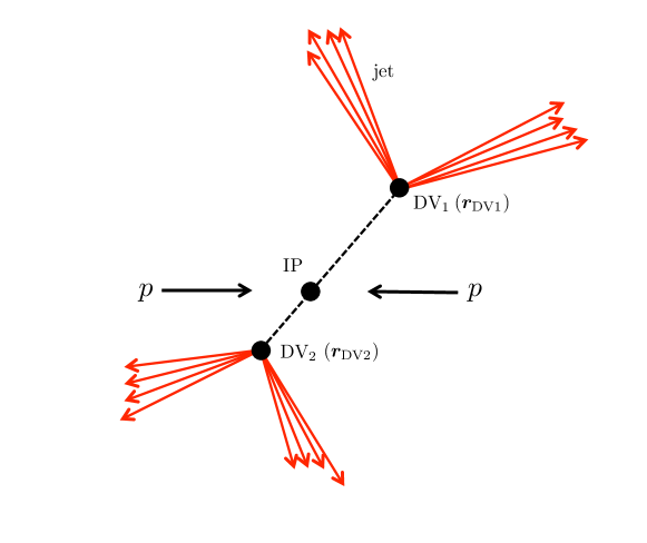
Figure 1: The event topology of metastable gluino decay. Here, ${\rm DV}_{1}$ and ${\rm DV}_{2}$ are two decay vertices of gluino, while IP is the interaction point.

As mentioned above, gluinos are pair produced and the decay of each gluino gives rise to two hard jets; this event topology is illustrated in Fig. 1. Considering this, we reconstruct displaced vertices in the metastable gluino decay events by using only tracks associated with four high-$p_{\text{T}}$ jets. The way of choosing these four high-$p_{\text{T}}$ jets, as well as the track conditions, will be given in Sec. 4. The reconstruction of the decay vertices in gluino decay events is complicated due to the fact that it is unclear which pair of jets is associated with the same vertex. In our analysis, we consider all three possible patterns of pairings out of the four jets and reconstruct a vertex for each pair using the method described above. For each pairing, we determine the positions of two decay vertices assuming that the jets in a pair originate from the same decay vertex; each decay vertex is determined with the tracks associated to the jets constituting the pair. We then choose the pairing that has the smallest value of $\chi^{2}$ defined by

$$\chi^{2}\equiv\frac{\sum_{i\in\text{trk}(\bm{v}_{1})}w_{i}\chi^{2}_{i}(\bm{v}_{1})+\sum_{j\in\text{trk}(\bm{v}_{2})}w_{j}\chi^{2}_{j}(\bm{v}_{2})}{\sum_{i\in\text{trk}(\bm{v}_{1})}w_{i}(\bm{v}_{1})+\sum_{j\in\text{trk}(\bm{v}_{2})}w_{j}(\bm{v}_{2})}~{},$$ (3)

where $\text{trk}(\bm{v}_{1,2})$ denotes the set of tracks associated with the vertex reconstructed at the position $\bm{v}_{1,2}$ for each pair of jets. Note that $\chi_{i}^{2}(\bm{v})$ is the squared standardized distance from the vertex $\bm{v}$, which is defined by Eq. (1). We employ the vertices obtained with this pairing, and denote their positions by $\bm{r}_{\text{DV1,2}}\equiv\bm{v}_{1,2}$. This new information of the position of the displaced vertices will be used to improve the metastable gluino searches in the following analysis.

3 Gluino phenomenology

As mentioned in the introduction, we consider a metastable gluino as a concrete example and study the effect of the new selection cut on the gluino searches. Here we assume that all of the squarks are much heavier than gluino and there is at least one neutralino which is lighter than the gluino. In this case, gluinos $\tilde{g}$ decay either in the tree-level three-body decay processes with the emission of a pair of quarks and a neutralino $\tilde{\chi}^{0}$ or chargino $\tilde{\chi}^{\pm}$, $\tilde{g}\to q\bar{q}\tilde{\chi}^{0},q\bar{q}^{\prime}\tilde{\chi}^{\pm}$, or in the one-loop two-body decay process where a gluino and a neutralino is emitted: $\tilde{g}\to g\tilde{\chi}^{0}$. It is found that if the gluino mass is $\gtrsim 2$ TeV, then the three-body decay processes dominate the two-body decay [2, 3, 4]. As the three-body decay processes are induced by the exchange of virtual heavy squarks, the amplitudes of these processes are suppressed by the squared masses of these heavy squarks, $m_{\tilde{q}}^{2}$. As a consequence, gluinos become long-lived if the squark masses are sufficiently heavy. To see this more quantitatively, we show an approximate formula for the decay length of gluinos:

$$c\tau_{\tilde{g}}\simeq 200\times\biggl{(}\frac{m_{\tilde{q}}}{10^{3}~{}\text{TeV}}\biggr{)}^{4}\biggl{(}\frac{m_{\tilde{g}}}{2~{}\text{TeV}}\biggr{)}^{-5}~{}\mu\text{m}~{},$$ (4)

where $m_{\tilde{g}}$ is the mass of gluino. In deriving this approximate formula, we have assumed that the gluino mainly decays into the first-generation quarks, the masses of bino and wino are much smaller than the gluino mass, and higgsinos are heavier than the gluino. In this case, $m_{\tilde{q}}$ corresponds to the mass of the first-generation squarks. From Eq. (4), we see that metastable gluinos with a decay length of $\gtrsim 100~{}\mu\text{m}$ are obtained if squarks lie around the PeV scale or higher.

In fact, the PeV-scale squarks are phenomenologically well motivated. First and foremost, with such heavy squarks (especially heavy stops), the observed value of the SM-like Higgs boson mass [91] can be explained within the minimal SUSY SM [92, 93, 94, 95, 96]. In addition, the contributions of SUSY particles to the flavor-changing neutral current processes, the electric dipole moments, and the dimension-five proton decay processes are all suppressed by heavy sfermion masses, and thus the experimental limits on such dangerous processes can easily be evaded [97, 98, 99, 100, 101, 102, 103, 104]. Even though squarks are as heavy as ${\cal O}(1)$ PeV, fermionic SUSY particles can naturally be around the TeV scale since their masses are protected by chiral symmetry. A simple framework to realize this split spectrum [105, 106, 107, 108, 109, 110] is provided by the so-called anomaly-mediated SUSY-breaking mechanism [105, 111], where gaugino masses are induced by quantum corrections and thus suppressed by a loop factor compared with the gravitino mass. This gives theoretical support for the split SUSY mass spectrum. A distinguished feature of this type of spectrum is that the lightest SUSY particle (LSP), which is one of the TeV-scale fermionic SUSY particles such as the neutral wino and higgsino, can be a promising candidate for dark matter in the Universe [112, 113]. These advantages have thus attracted a lot of attentions [114, 115, 116, 117, 118, 119, 120, 121] especially after the early stage of the LHC run. In such a split spectrum, gluino may also lie around the TeV scale and be within the reach of the LHC and/or a future hadron collider. Gluinos in this case are expected to have a sizable decay length according to Eq. (4)—in this sense, a metastable gluino may be regarded as a smoking-gun signature of the split-type SUSY spectrum and the detection of such a gluino enables us to confirm this scenario experimentally. Moreover, since the lifetime of metastable gluinos reflects the squark mass scale, we may probe this via the precise measurements of the gluino decay length, even though we cannot produce squarks directly at colliders. We discuss this possibility in more detail in Sec. 4.4.

If the gaugino masses are induced mainly by the anomaly mediation, the gaugino mass spectrum is determined by the gauge-coupling beta functions; in particular, one finds that the LSP is the neutral wino in this case. On the other hand, if there are other contributions which are comparable to the anomaly-mediation contribution in size, the gaugino mass spectrum can deviate from the anomaly-mediation relation and, in fact, the spectrum could take any form. For example, threshold corrections by heavy Higgs bosons/higgsinos [122, 105] and some extra matter fields [123, 124, 125, 126, 127, 128, 129] give rise to such contributions. Considering this, we regard both the gluino and LSP masses as free parameters in what follows.

An interesting possibility of gaugino mass spectrum is that the LSP (say bino) is degenerate with gluino in mass with a mass splitting of $\sim 100$ GeV. In this case, the annihilation cross section of the LSP in the early Universe is strongly enhanced by the coannihilation effect [130], which has significant implications for the relic abundance of the LSP. In fact, it is found that the relic abundance of the bino LSP agrees to the observed dark matter density if the mass difference between bino and gluino is $\lesssim 100$ GeV [131, 132, 133, 134, 135, 30, 136, 137]. Motivated by this observation, we will also consider such a degenerate mass spectrum in our analysis.

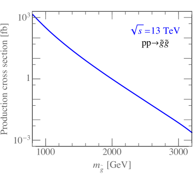
(a) 13 TeV

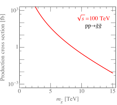
(b) 100 TeV

Figure 2: The pair-production cross sections of gluinos as functions of the gluino mass.

At hadron colliders, gluinos are pair-produced through the strong interactions, and the cross section of this process is unambiguously determined if squarks are heavy enough. We show the pair-production cross sections of gluinos as functions of the gluino mass for $\sqrt{s}=13$ and 100 TeV in Fig. 2(a) and Fig. 2(b), respectively. They are computed using the CTEQ6.6 PDF set [138] with the next-to-leading order QCD corrections included and soft gluon emission resummed at the next-to-leading logarithmic accuracy [139]. We will use these production cross sections in the following analyses.

4 13 TeV LHC

Now we study how far we may extend the reach of the prompt-decay gluino searches at the 13 TeV LHC using a new cut based on the reconstruction of displaced vertices. We first describe our MC simulation procedure in Sec. 4.1, which is followed by the summary of the event selection criteria used in this analysis in Sec. 4.2. We then show the prospects of the new event-selection cut in Sec. 4.3. Finally, in Sec. 4.4, we discuss the possibility of measuring the lifetime of gluino in the future LHC experiments.

4.1 MC simulation

$m_{\tilde{g}}$	$1000,\,1200,\,\ldots,\,3200$ GeV
$m_{\tilde{\chi}_{1}^{0}}$	$100$ GeV,
	$(0.2,\,0.4,\,0.6,\,0.7,\,0.8)\times m_{\tilde{g}}$,
	$m_{\tilde{g}}-(150\,{\rm GeV},\,100\,{\rm GeV},\,50\,{\rm GeV},\,25\,{\rm GeV})$
$c\tau_{\tilde{g}}$	$0,\,50,\,100,\,200,\,500,\,1000,\,3000$ ${\rm\mu m}$,
	$1\times 10^{4},\,3\times 10^{4},\,1\times 10^{5},\,3\times 10^{5},\,1\times 10^{6}$ ${\rm\mu m}$

Table 1: Sample points for signal events. We generate 50000 events for each sample point.

In the following analysis, both signal and background events are generated with MC simulations. For signal events, we use MadGraph5_aMC@NLO v2 [140] and PYTHIA v8.2 [141], and generate 50000 events for each model point categorized in terms of the gluino mass $m_{\tilde{g}}$, the LSP mass $m_{\tilde{\chi}_{1}^{0}}$, and the gluino decay length $c\tau_{\tilde{g}}$; sample points with this categorization are summarized in Table 1. In generating the signal events, (i) the gluinos are forced to decay at the interaction point, then (ii) the decay points are spatially shifted by the flight lengths of the parent gluinos, whose probability distribution is determined from the lifetime of gluino $\tau_{\tilde{g}}$. All the trajectories of the decay products of the parent gluinos are shifted accordingly. The number of signal event samples is normalized according to the production cross section given in Fig. 2(a). In our analysis, gluino is assumed to decay only into the first-generation quarks. In reality, gluino may also have sizable decay fractions into the other two generations of quarks, especially top quark when the stop mass is similar to or smaller than the first-generation squark masses. We will briefly discuss such cases in Sec. 6. Moreover, we neglect the hadronization effect of gluinos as it is known that the energy and momentum of the resultant $R$-hadrons are almost the same as those of the produced gluinos, for a gluino mass of ${\cal O}(1)$ TeV [1, 142].

As for the SM background events, we consider the production processes of the electroweak gauge bosons ($W^{\pm}$ and $Z$) and top-quark pairs ($t\bar{t}$). We do not consider the fully hadronic decay processes of these particles since we require a large missing energy and thus such events are expected to be efficiently eliminated. In addition, we do not take account of diboson production and multi-jet processes as they are found to be subdominant [143]. For the $Z$ boson production channel, the matrix elements are calculated with up to four additional partons. Due to the limitation of our available computational resources, we include only up to three and one extra partons for the $W$ and $t\bar{t}$ production processes, respectively, which are subdominant compared with the $Z$ boson production process. (We also studied these processes with one more parton. Although the number of generated events is not enough for our analysis of the gluino search, we observed that the number of SM background does not seem to be significantly changed even if we add one more parton to these samples.) The samples with different number of additional partons are merged using the five flavor MLM matching scheme with $k_{t}$ jets [144]. Here we adopt the shower-$k_{t}$ scheme and set the matching parameter ${\rm QCUT}={\rm XQCUT}$ to $40$ GeV for the $Z$ and $W$ production processes and $80$ GeV for the $t\bar{t}$ production process, following Ref. [145]. All generated samples are passed to PYTHIA v8.2 [141] and then DELPHES v3 [146] for the purpose of parton showering and fast detector simulation, respectively.

	bin $\alpha$	0	1	2	3	4
$H_{T,0}^{\rm max}(\alpha)$	(GeV)	$600$	$1200$	$2000$	$2900$	$\infty$
$\sigma_{\text{matched}}(\alpha)$	(fb)	$8.85{\scriptstyle\times 10^{2}}$	$5.50{\scriptstyle\times 10^{2}}$	$66.5$	$6.6$	$0.83$
$N_{\text{matched}}(\alpha)$	$(\times 10^{3})$	$4.6$	$53.6$	$65.3$	$198$	$28.8$
$\mathcal{L}_{\rm gen}(\alpha)$	(${\rm ab}^{-1}$)	$5.23{\scriptstyle\times 10^{-3}}$	$0.0975$	$0.982$	$29.9$	$34.6$

(a) $Z\rightarrow\nu\bar{\nu}+4j$.

	bin $\alpha$	0	1	2	3	4
$H_{T,0}^{\rm max}(\alpha)$	(GeV)	$600$	$1200$	$2000$	$2900$	$\infty$
$\sigma_{\text{matched}}(\alpha)$	(fb)	$1.22{\scriptstyle\times 10^{4}}$	$7.85{\scriptstyle\times 10^{2}}$	$55.7$	$4.65$	$0.54$
$N_{\text{matched}}(\alpha)$	$(\times 10^{3})$	$214$	$325$	$574$	$135$	$133$
$\mathcal{L}_{\rm gen}(\alpha)$	(${\rm ab}^{-1}$)	$0.0176$	$0.413$	$10.3$	$29.1$	$247$

(b) $Z\rightarrow\nu\bar{\nu}+0,1,2,3\,j$.

	bin $\alpha$	0	1	2	3	4
$H_{T,0}^{\rm max}(\alpha)$	(GeV)	$600$	$1200$	$2000$	$2900$	$\infty$
$\sigma_{\text{matched}}(\alpha)$	(fb)	$6.28{\scriptstyle\times 10^{4}}$	$1.04{\scriptstyle\times 10^{3}}$	$74.4$	$6.05$	$0.69$
$N_{\text{matched}}(\alpha)$	$(\times 10^{3})$	$280$	$223$	$212$	$207$	$205$
$\mathcal{L}_{\rm gen}(\alpha)$	(${\rm ab}^{-1}$)	$4.46{\scriptstyle\times 10^{-3}}$	$0.214$	$2.85$	$34.1$	$300$

(c) $Z\rightarrow\ell\bar{\ell}+0,1,2,3\,j$

Table 2: The upper edge value of $H_{T,0}$, $H_{T,0}^{\rm max}(\alpha)$, the leading-order matched cross section, $\sigma_{\text{matched}}$, the number of samples after matching, $N_{\text{matched}}$, and the equivalent luminosity, $\mathcal{L}_{\rm gen}$, in each $H_{T,0}$ bin for the $Z$-boson production process.

	bin $\alpha$	0	1	2	3	4	5
$H_{T,0}^{\rm max}(\alpha)$	(GeV)	$400$	$900$	$1600$	$2500$	$3400$	$\infty$
$\sigma_{\text{matched}}(\alpha)$	(fb)	$5.15{\scriptstyle\times 10^{5}}$	$3.15{\scriptstyle\times 10^{4}}$	$2.10{\scriptstyle\times 10^{3}}$	$1.74{\scriptstyle\times 10^{2}}$	$14.2$	$1.92$
$N_{\text{matched}}(\alpha)$	$(\times 10^{3})$	$286$	$233$	$2180$	$1680$	$414$	$206$
$\mathcal{L}_{\rm gen}(\alpha)$	(${\rm ab}^{-1}$)	$5.5{\scriptstyle\times 10^{-4}}$	$7.41{\scriptstyle\times 10^{-3}}$	$1.04$	$9.64$	$29.2$	$107$

Table 3: Same as in Table 2, but for the $W$ production process.

	bin $\alpha$	0	1	2	3	4	5
$H_{T,0}^{\rm max}(\alpha)$	(GeV)	$600$	$1100$	$1700$	$2400$	$3200$	$\infty$
$\sigma_{\text{matched}}(\alpha)$	(fb)	$7.43{\scriptstyle\times 10^{4}}$	$5.64{\scriptstyle\times 10^{3}}$	$4.26{\scriptstyle\times 10^{2}}$	$36.8$	$3.43$	$0.34$
$N_{\text{matched}}(\alpha)$	$(\times 10^{3})$	$154$	$1220$	$1280$	$177$	$182$	$186$
$\mathcal{L}_{\rm gen}(\alpha)$	(${\rm ab}^{-1}$)	$2.08{\scriptstyle\times 10^{-3}}$	$0.216$	$2.99$	$4.81$	$53.0$	$552$

(a) $t\bar{t}\rightarrow$ (semi-leptonic)$+0,1j$.

	bin $\alpha$	0	1	2	3
$H_{T,0}^{\rm max}(\alpha)$	(GeV)	$800$	$1400$	$2100$	$\infty$
$\sigma_{\text{matched}}(\alpha)$	(fb)	$418$	$38.9$	$3.74$	$0.34$
$N_{\text{matched}}(\alpha)$	$(\times 10^{3})$	$41$	$48$	$97$	$49$
$\mathcal{L}_{\rm gen}(\alpha)$	(${\rm ab}^{-1}$)	$0.0980$	$1.22$	$26.0$	$146$

(b) $t\bar{t}\rightarrow$ (leptonic)$+0,1j$.

Table 4: Same as in Table 2, but for the $t\bar{t}$ production process.

In new physics searches with a large integrated luminosity, it is the distribution tail of discriminating variables from the SM background processes that affects the sensitivities of these searches. A simulation of such tails in general requires a huge amount of background samples. To deal with this difficulty, we use the technique described in Ref. [145]. In this method, the generator-level phase space is divided into several regions, and MC samples are separately generated and matched for each region. The generated samples are then combined with each other after multiplied by some weight factor. In our analysis, we divide the generator-level phase space into bins numbered by $\alpha=0,1,2,\dots$, in terms of the scalar sum of $p_{\text{T}}$ of partons in each event:

$$H_{T,0}\equiv\sum_{\text{partons}}p_{\text{T}}.$$ (5)

We show the values of the upper edge of each bin $\alpha$, denoted by $H_{T,0}^{\text{max}}(\alpha)$, for the $Z$, $W$, and $t\bar{t}$ production processes in Tables 2, 3, and 4, respectively. Here, the width of the bin $\alpha+1$ is determined such that the corresponding cross section is $\simeq 1/10$ of that of the bin $\alpha$. We also give the leading-order matched cross section $\sigma_{\text{matched}}$, the number of samples after matching $N_{\text{matched}}$, and the equivalent luminosity $\mathcal{L}_{\rm gen}=N_{\text{matched}}/\sigma_{\text{matched}}$ in these tables. When generating these samples, we impose a generator-level cut of $|\sum_{{\rm all}\,\nu}\bm{p}_{\rm T}|>200$ GeV for $Z\rightarrow\nu\bar{\nu}$ and $|\sum_{{\rm all}\,l,\nu}\bm{p}_{\rm T}|>100$ GeV for the other processes. We then define the weight $w_{\alpha}$ for the samples in the bin $\alpha$ by

$$w_{\alpha}\equiv\frac{\sigma_{\text{matched}}(\alpha)}{N_{\text{matched}}(\alpha)}~{},$$ (6)

and all samples in the bins are added by using these weights.

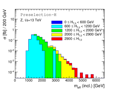
(a) $Z$ boson production

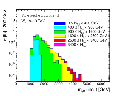
(b) $W$ boson production

Figure 3: Distributions of $m_{\text{eff}}(\text{incl.})$ with preselection-H required. Contributions from different $H_{T,0}$ bins are filled with different colors.

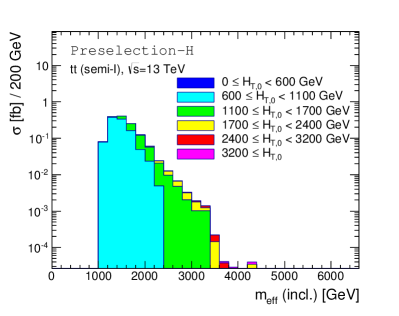
(a) Semi-leptonic $t\bar{t}$ decay

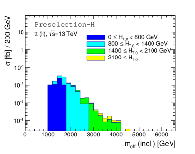
(b) Leptonic $t\bar{t}$ decay

Figure 4: Same as in Fig. 3, but for the $t\bar{t}$ production process.

By using the samples obtained above, we generate the distribution of $m_{\text{eff}}(\text{incl.})$ for each process, where $m_{\text{eff}}(\text{incl.})$ is defined as the scalar sum of the missing transverse energy $E_{\rm T}^{\rm(miss)}$ and the transverse momenta of all jets with $p_{\rm T}>50$ GeV; the results are given in Figs. 3 and 4. These distributions are obtained for events passing a selection requirement Preselection-H, whose definition is found in Table 5 in the next section. We will use $m_{\text{eff}}(\text{incl.})$ to define signal regions in the following analyses. From these figures, we find that there is a correlation between $H_{T,0}$ and $m_{\text{eff}}(\text{incl.})$. In addition, we find a sizable number of events in the tails of the distributions, which smoothly spread out from the bulk of the distributions. These observations indicate that the division of the generator-level phase space in terms of $H_{T,0}$ offers an adequate way to estimate the number of events in signal regions which are defined by the values of $m_{\text{eff}}(\text{incl.})$.

For the definition of the objects such as charged tracks, jets, and charged leptons, we basically follow Ref. [143]. We require $p_{\text{T}}>1$ GeV and $|\eta|<2.5$ for the reconstruction of a charged track, and reject it if the production point of the particle associated with the charged track is outside the innermost pixel layer, which is located at $|\bm{r}_{\text{T}}|=33.25$ mm. These requirements are intended to remove tracks with poor measurement quality. Jets are clustered using FastJet v3.1 [147] with a jet radius parameter of $0.4$ and required to satisfy $p_{\rm T}>20$ GeV and $|\eta|<2.8$. For leptons, we require $p_{\rm T}>7$ GeV, and $|\eta|<2.47$ $(2.7)$ for electrons (muons).

As we will mention in the next section, we require neither electrons nor muons be reconstructed in our analysis. In this case, the SM background processes listed above can contribute to the signal regions only if all of the leptons in the processes fail to be reconstructed. To take account of this, we introduce the reconstruction probability of an electron (muon), $p^{e(\mu)}_{\text{reco.}}(p_{\text{T}},\eta)$, which we take from DELPHES v3 [146]. We then multiply the weight $w_{\alpha}$ in Eq. (6) by a factor of $\prod_{{\rm all}\,e_{i}}(1-p_{{\rm reco.}}^{e_{i}})\times\prod_{{\rm all}\,\mu_{i}}(1-p_{{\rm reco.}}^{\mu_{i}})$ when we require the absence of electrons and muons.

To validate our MC simulations, we compute the expected number of background events as well as the expected $95$% confidence level (CL) exclusion limit on gluino mass for an integrated luminosity of $36.1\,{\rm fb}^{-1}$ at the 13 TeV LHC. We use the kinematical selection category called Meff-4j-3000 given in Ref. [143]. We then find the expected number of background events to be $1.4$ and the exclusion limit on the gluino mass to be $1960$ GeV. Comparing these results with the ones reported by the ATLAS collaboration [143]—$2.0$ and $2030$ GeV, respectively—we can safely conclude that our MC simulation satisfactorily reproduces the ATLAS results.

4.2 Event selection criteria

Requirement	L	M	H
Number of jets with $p_{\rm T}>50$ GeV	$\geq 4$
$E_{\rm T}^{\rm(miss)}$ [GeV]	$>250$
$p_{\rm T}(j_{1})$ [GeV]	$>200$
$p_{\rm T}(j_{4})$ [GeV]	$>100$	$>100$	$>150$
$|\eta(j_{i=1,2,3,4})|$	$<1.2$	$<2.0$	$<2.0$
$\Delta\phi(j_{p_{\rm T}>50\,{\rm GeV}},E_{\rm T}^{\rm(miss)})_{\rm min}$	$>0.4$
$E_{\rm T}^{\rm(miss)}/m_{\rm eff}(4)$	$>0.3$	$>0.25$	$>0.2$
Aplanarity	$>0.04$

Table 5: Definition of preselection-L, M, H. Besides these criteria, we require that neither electrons nor muons be reconstructed.

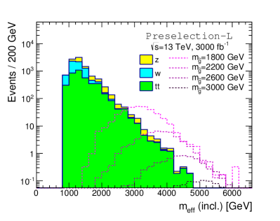
(a) Preselection-L

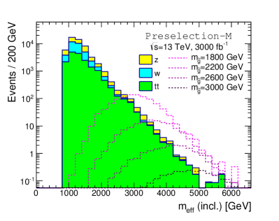
(b) Preselection-M

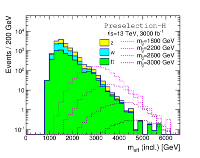
(c) Preselection-H

Figure 5: Distributions of $m_{\text{eff}}(\text{incl.})$ for the SM background and gluino events. We set the LSP mass to be 100 GeV.

In our analysis, we impose a new event-selection cut using the information of displaced vertices in addition to the ordinary selection criteria based on kinematics. We further try to optimize the kinematic-based cuts as the new selection cut is expected to reduce the SM background efficiently. To that end, we first divide the kinematic-based selection criteria into two classes; $m_{\text{eff}}(\text{incl.})$, which is to be varied to optimize the event selection, and the other criteria adopted in Ref. [143], which we call the preselection. Moreover, we divide the preselection into three classes, preselection-L, -M, and -H, and use one of them for each sample point so that the sensitivity is maximized. We summarize the preselection criteria in Table 5. Here, $p_{\rm T}(j_{i})$ denotes the transverse momentum of $i$-th jet, $\Delta\phi$ is the azimuthal angle between the jet and the missing energy, and $m_{\rm eff}(4)$ is the scalar sum of $E_{\rm T}^{\rm(miss)}$ and the transverse momenta of the leading $4$-jets. The requirements on $\Delta\phi$ and $E_{\rm T}^{\rm(miss)}/m_{\rm eff}(4)$ were imposed to reduce the contributions from QCD multi-jet processes in Ref. [143]—although such multi-jet processes are not included in the present analysis, we still impose these requirements since they are also able to reject background events from the semi-leptonically decaying $t$ and $\bar{t}$ efficiently. The definition of aplanarity can be found in Refs. [148, 149]; if a distribution of jets is highly directional, then the value of aplanarity gets close to zero, while if it is completely isotropic then this is equal to $1/2$. In addition to these kinematical selection criteria, we require that neither electrons nor muons be reconstructed. In Fig. 5, we give the distributions of $m_{\text{eff}}(\text{incl.})$ for the SM background and gluino events with each preselection imposed. Here, we set the LSP mass to be 100 GeV. These figures show that we may effectively select gluino events while eliminating the SM background if we require a large $m_{\text{eff}}(\text{incl.})$. The size of this cut will be chosen so that the sensitivity is maximized, as we see in the subsequent section.

Now we discuss a selection criterion based on the reconstruction of displaced vertices. As described in Sec. 2, we reconstruct vertices using charged tracks associated with the decay product. The resolutions of impact parameters, which determine the resolution of vertex reconstruction, are obtained by fitting Eq. (2) onto the experimental results given by the ATLAS collaboration [87, 88]. As we mentioned in Sec. 4.1, only the tracks with $p_{\text{T}}>1$ GeV are used in this analysis. Performing the fit in this range, we determine the parameters in Eq. (2) as $\sigma_{d_{0}}(\infty)=23~{}\mu\text{m}$, $\sigma_{z_{0}\sin\theta}(\infty)=78~{}\mu\text{m}$, $p_{d_{0}}=3.1$ GeV, and $p_{z_{0}\sin\theta}=1.6$ GeV.

As we discussed in Sec. 2, we use four high-$p_{\text{T}}$ jets to reconstruct displaced vertices generated in gluino-decay events. For this purpose, we basically choose the four-highest $p_{\text{T}}$ jets. We further require that the tracks in these jets satisfy $d_{0}<10$ mm and $|z_{0}|<320$ mm in order to focus on decays that occur inside the inner detector. However, if one of these four jets contains no track which satisfies the above conditions, then we add the fifth-highest $p_{\rm T}$ jet to the vertex reconstruction analysis. If the number of jets which contain tracks satisfying the criteria is smaller than four among these five jets, then we conclude that the reconstruction of vertices fails in such an event.

As our main focus is on displaced vertices located inside the innermost pixel layer, vertices generated by hadronic interactions in the detector materials rarely contribute to the background. To assure this, we reject events in which a vertex is reconstructed inside the detector materials: i.e., $22~{}{\rm mm}\leq|(\bm{r}_{\rm DV1,2})_{\rm T}|\leq 25$ mm, $29~{}{\rm mm}\leq|(\bm{r}_{\rm DV1,2})_{\rm T}|\leq 38$ mm, $46~{}{\rm mm}\leq|(\bm{r}_{\rm DV1,2})_{\rm T}|\leq 73$ mm, $84~{}{\rm mm}\leq|(\bm{r}_{\rm DV1,2})_{\rm T}|\leq 111$ mm, or $|(\bm{r}_{\rm DV1,2})_{\rm T}|\geq 120~{}{\rm mm}$ [89, 150, 151, 152]. In the absence of this possibility, the displaced vertices from the SM processes are mainly caused by the misinterpretation of non-displaced vertices due to the limited resolution of track impact parameters, which we take into account in a manner discussed in Sec. 2.

In the metastable gluino production processes under consideration, we do not expect that particles with hard momenta are generated at the primary interaction point (except those from initial state radiation), as the metastable gluinos decay after they flew away from the primary interaction point. For this reason, we do not try to determine the position of the primary interaction point in each event. Instead, we use the distance between the two reconstructed vertices as a discriminator. As for the definition of the distance, we try the following three candidates and adopt the one which yields the best sensitivity for each sample point: $|\bm{r}_{\rm DV1}-\bm{r}_{\rm DV2}|$, $|(\bm{r}_{\rm DV1}-\bm{r}_{\rm DV2})_{\rm T}|$, and $|(\bm{r}_{\rm DV1}-\bm{r}_{\rm DV2})_{z}|$, where $\bm{r}_{\rm DV1,2}$ are the position vectors of the displaced vertices defined in Sec. 2, and T and $z$ stand for the transverse and $z$ directions, respectively.

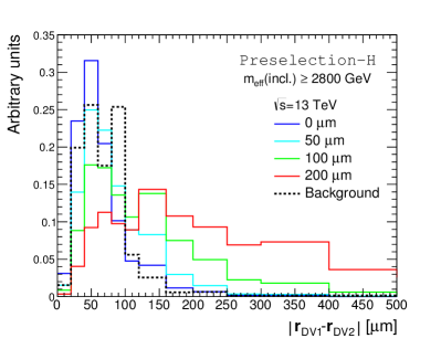
(a) $|\bm{r}_{\rm DV1}-\bm{r}_{\rm DV2}|$ distribution

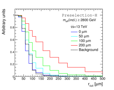
(b) Efficiency

Figure 6: The distributions of $|\bm{r}_{\rm DV1}-\bm{r}_{\rm DV2}|$ and the fractions to pass the selection cut $|\bm{r}_{\rm DV1}-\bm{r}_{\rm DV2}|>r_{\rm cut}$ for a gluino with $m_{\tilde{g}}=3$ TeV and different values of $c\tau_{\tilde{g}}$, shown in the solid lines. The distributions for the SM background events are also shown in the dotted lines. We have imposed preselection-H and $m_{\rm eff}({\rm incl.})>2800\,\,{\rm GeV}$.

In Fig. 6(a), we show the $|\bm{r}_{\rm DV1}-\bm{r}_{\rm DV2}|$ distribution of signal events for a gluino with $m_{\tilde{g}}=3$ TeV and different values of the decay distance $c\tau_{\tilde{g}}$ in the solid lines. The distribution for the SM background events is also shown in the dotted line. Figure 6(b) shows a fraction of events passing a selection cut of $|\bm{r}_{\rm DV1}-\bm{r}_{\rm DV2}|>r_{\rm cut}$ as a function of $r_{\rm cut}$. For these simulations, we have imposed preselection-H and $m_{\rm eff}({\rm incl.})>2800\,\,{\rm GeV}$. Notice that the distribution of the SM background deviates from the signal distribution with $c\tau_{\tilde{g}}=0$. This is because the flavor content of jets in the SM background sample is different from that in the signal event sample. In the signal events, gluinos are forced to decay into only the first-generation quarks as we mentioned above. In the SM background events, on the other hand, jets may also be induced by heavy flavor quarks, which then contain metastable hadrons; for example, the typical decay length of $B$ mesons is about $400\,{\rm\mu m}$ and these mesons can fly over a few mm when they are highly boosted. Decay products of such metastable hadrons may form a secondary vertex and deteriorate resolution of the vertex reconstruction position. We however note that our vertex reconstruction method is actually robust against the presence of metastable hadrons. A jet originating from a heavy flavor quark contains not only metastable hadrons such as $B$ mesons but also other many hadrons emitted during hadronization. Since our vertex reconstruction algorithm chooses as the vertex position a point at which tracks are most densely concentrated, it is less likely to identify a secondary vertex caused by a metastable hadron as the reconstructed vertex. For the same reason, our vertex reconstruction method is less affected by pile-up events as well, especially if we reconstruct vertices using only tracks in high-$p_{\rm T}$ jets as we do in our analysis. The effect of pile-up events on kinematical selection cuts is also expected to be small [153]. Considering these, we do not include the pile-up effects in our analysis.

The plots in Fig. 6 show that if we set $r_{\rm cut}$ to be $\gtrsim 100~{}\mu{\rm m}$, then a significant fraction of the SM background fails to pass the selection cut while a sizable number of signal events for $c\tau_{\tilde{g}}\gtrsim 100~{}\mu{\rm m}$ still remain after the selection cut. This observation indicates that this cut may be useful to probe a gluino with a decay length of $c\tau_{\tilde{g}}\gtrsim 100~{}\mu{\rm m}$, which we demonstrate in the subsequent section.

4.3 Prospects

Selection	Requirements
Preselection	$\in$ (preslection-L, M, H)
Lepton veto	No reconstructed electrons and muons
Material veto	No vertices reconstructed in material regions:
	i.e. (in units of mm)
	$|(\bm{r}_{\rm DV})_{\rm T}|\notin$ $(22,25)$, $(29,38)$, $(46,73)$, $(84,111)$, $(120,\infty)$
$m_{\rm eff}({\rm incl.})$ cut	Require $m_{\rm eff}({\rm incl.})>\left(m_{\rm effcut}\right)_{\rm optimal}$
	over
	$m_{\rm effcut}\in(1000~{}{\rm GeV},10^{4}~{}{\rm GeV})$
$\Delta r_{\rm DV}$ cut	Require $\Delta r_{\rm DV}>\left(r_{\rm cut}\right)_{\rm optimal}$
	over
	$\Delta r_{\rm DV}\in(\left|\Delta\bm{r}_{\rm DV}\right|,\left|\left(\Delta\bm{r}_{\rm DV}\right)_{\rm T}\right|,\left|\left(\Delta\bm{r}_{\rm DV}\right)_{\rm z}\right|)$
	$r_{\rm cut}\in(0,2\times 10^{5}{\rm\mu m})$

Table 6: Summary of event selection criteria.

Let us summarize the event selection criteria we use in the following analysis. After we apply one of the preselections, preselection-L,-M,-H, we further require

$$m_{\rm eff}({\rm incl.})>\left(m_{\rm effcut}\right)_{\rm optimal}\quad\text{and}\quad\Delta r_{\rm DV}>\left(r_{\rm cut}\right)_{\rm optimal}$$ (7)

where $\Delta r_{\rm DV}$ is one of the discriminators proposed in the previous section, i.e., $\Delta r_{\rm DV}=|\Delta\bm{r}_{\rm DV}|$, $|(\Delta\bm{r}_{\rm DV})_{\text{T}}|$, or $|(\Delta\bm{r}_{\rm DV})_{z}|$, where $\Delta\bm{r}_{\rm DV}\equiv\bm{r}_{\rm DV1}-\bm{r}_{\rm DV2}$. We adopt the one which leads to the best sensitivity for a given sample point. We vary the cut parameters $m_{\rm effcut}$ and $r_{\rm cut}$ in Eq. (7) from $1000$ GeV to $10^{4}$ GeV and from $0~{}\mu\text{m}$ to $2\times 10^{5}~{}{\rm\mu m}$, respectively, and employ the values which maximize the performance. These event selection criteria are listed in Table 6.

Now we study the performance of the new selection cut based on the reconstruction of displaced vertices. To that end, we evaluate the discovery reach and exclusion limit for metastable gluino searches and compare them with the existing results from the prompt decay searches. For exclusion limits, we compute the expected 95% confidence level (CL) limits on the gluino mass using the $CL_{s}$ prescription [154, 155]. For the discovery reach, we compute the expected significance of discovery $Z_{0}$ [156]:

$$Z_{0}=\sqrt{2\left\{\left(S+B\right)\log\left(1+S/B\right)-S\right\}}~{},$$ (8)

where $S$ and $B$ are the expected numbers of signal and background events, respectively. We then require both $Z_{0}$ and $S$ to be larger than $5$ for the discovery.

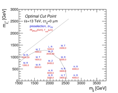
(a) $c\tau_{\tilde{g}}=0~{}{\rm\mu m}$

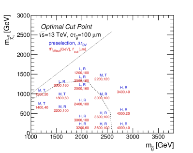
(b) $c\tau_{\tilde{g}}=100~{}{\rm\mu m}$

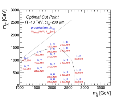
(c) $c\tau_{\tilde{g}}=200~{}{\rm\mu m}$

(d) $c\tau_{\tilde{g}}=500~{}{\rm\mu m}$

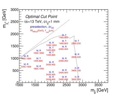
(e) $c\tau_{\tilde{g}}=1~{}{\rm mm}$

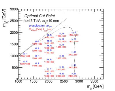
(f) $c\tau_{\tilde{g}}=10~{}{\rm mm}$

Figure 7: Optimal cut values ($(m_{\rm effcut})_{\rm optimal}$, $(r_{\rm cut})_{\rm optimal}$), the preselection (L, M, H), and the discriminator $\Delta r_{\rm DV}$ (R, T, Z) for each sample point with various $c\tau_{\tilde{g}}$, with an integrated luminosity of $3000~{}{\rm fb}^{-1}$. The expected $5\sigma$ discovery reaches for gluinos are also shown in the dashed lines.

In Fig. 7, we show optimal cut values ($(m_{\rm effcut})_{\rm optimal}$, $(r_{\rm cut})_{\rm optimal}$), the preselection (L, M, or H), and the discriminator $\Delta r_{\rm DV}$ (R, T, or Z) for each sample point with various $c\tau_{\tilde{g}}$, with an integrated luminosity of $3000~{}{\rm fb}^{-1}$. Here, for the discriminator $\Delta r_{\rm DV}$, R, T, and Z represent $|\Delta\bm{r}_{\rm DV}|$, $|(\Delta\bm{r}_{\rm DV})_{\text{T}}|$, and $|(\Delta\bm{r}_{\rm DV})_{z}|$, respectively. They are obtained so that the expected significance $Z_{0}$ is maximized. The expected $5\sigma$ discovery reaches for gluinos are also shown in the dashed lines, which we discuss in more detail below. It is found that the new selection cut allows us to relax the kinematic selection cut on $m_{\rm eff}({\rm incl.})$ considerably, especially for gluinos with a long lifetime. As for the optimization of $(r_{\rm cut})_{\rm optimal}$, $(r_{\rm cut})_{\rm optimal}\simeq c\tau_{\tilde{g}}$ tends to be favored for gluinos with a sub-millimeter decay length.

	$Z$	$W$	$t\bar{t}$	total
preselection-H  $(\times 10^{3})$	$4.7{\scriptstyle~{}\pm 0.3}$	$4.1{\scriptstyle~{}\pm 0.6}$	$4.5{\scriptstyle~{}\pm 0.2}$	$13.3{\scriptstyle~{}\pm 0.7}$
$m_{\rm eff}({\rm incl.})>3600$ GeV	$12.5{\scriptstyle~{}\pm 1}$	$4.1{\scriptstyle~{}\pm 0.7}$	$1.6{\scriptstyle~{}\pm 0.4}$	$18.2{\scriptstyle~{}\pm 1}$
$\bigl{|}\bm{r}_{\rm DV1}-\bm{r}_{\rm DV2}\bigr{|}>80~{}{\rm\mu m}$	$2.1{\scriptstyle~{}\pm 0.4}$	$0.8{\scriptstyle~{}\pm 0.4}$	$0.2{\scriptstyle~{}\pm 0.1}$	$3.2{\scriptstyle~{}\pm 0.6}$
$\bigl{|}\bm{r}_{\rm DV1}-\bm{r}_{\rm DV2}\bigr{|}>160~{}{\rm\mu m}$	$0.1{\scriptstyle~{}\pm 0.1}$	$<0.1$	$<0.1$	$0.1{\scriptstyle~{}\pm 0.1}$
$\bigl{|}\bm{r}_{\rm DV1}-\bm{r}_{\rm DV2}\bigr{|}>200~{}{\rm\mu m}$	$0.1{\scriptstyle~{}\pm 0.1}$	$<0.1$	$<0.1$	$0.1{\scriptstyle~{}\pm 0.1}$

(a) The expected number of background events.

	$c\tau_{\tilde{g}}=0$	$c\tau_{\tilde{g}}=200~{}{\rm\mu m}$	$c\tau_{\tilde{g}}=500~{}{\rm\mu m}$	$c\tau_{\tilde{g}}=1~{}{\rm mm}$
preselection-H	$8.2{\scriptstyle~{}\pm 0.1}$
$m_{\rm eff}({\rm incl.})>3600$ GeV	$6.9{\scriptstyle~{}\pm 0.1}$
$\bigl{|}\bm{r}_{\rm DV1}-\bm{r}_{\rm DV2}\bigr{|}>80~{}{\rm\mu m}$	$1.6{\scriptstyle~{}\pm 0.04}$	$5.3{\scriptstyle~{}\pm 0.1}$	$6.3{\scriptstyle~{}\pm 0.1}$	$6.6{\scriptstyle~{}\pm 0.1}$
$\bigl{|}\bm{r}_{\rm DV1}-\bm{r}_{\rm DV2}\bigr{|}>160~{}{\rm\mu m}$	$0.2{\scriptstyle~{}\pm 0.01}$	$2.9{\scriptstyle~{}\pm 0.1}$	$5.1{\scriptstyle~{}\pm 0.1}$	$5.9{\scriptstyle~{}\pm 0.1}$
$\bigl{|}\bm{r}_{\rm DV1}-\bm{r}_{\rm DV2}\bigr{|}>200~{}{\rm\mu m}$	$<0.1$	$2.2{\scriptstyle~{}\pm 0.1}$	$4.5{\scriptstyle~{}\pm 0.1}$	$5.6{\scriptstyle~{}\pm 0.1}$

(b) The expected number of signal events for $m_{\tilde{g}}=2800$ GeV and $m_{\tilde{\chi}_{1}^{0}}=100$ GeV with different values of $c\tau_{\tilde{g}}$.

Table 7: The expected number of background (a) and signal (b) events for an integrated luminosity of $\mathcal{L}=3000~{}{\rm fb}^{-1}$. We set the masses of gluino and the LSP to be $2800$ GeV and $100$ GeV, respectively.

	$Z$	$W$	$t\bar{t}$	total
preselection-M  $(\times 10^{4})$	$1.7{\scriptstyle~{}\pm 0.10}$	$1.7{\scriptstyle~{}\pm 0.22}$	$1.8{\scriptstyle~{}\pm 0.05}$	$5.2{\scriptstyle~{}\pm 0.25}$
$m_{\rm eff}({\rm incl.})>2400$ GeV	$357{\scriptstyle~{}\pm 41}$	$148{\scriptstyle~{}\pm 13}$	$37{\scriptstyle~{}\pm 5}$	$542{\scriptstyle~{}\pm 44}$
$\bigl{|}\bm{r}_{\rm DV1}-\bm{r}_{\rm DV2}\bigr{|}>160~{}{\rm\mu m}$	$8.2{\scriptstyle~{}\pm 4}$	$3.6{\scriptstyle~{}\pm 1}$	$0.5{\scriptstyle~{}\pm 0.2}$	$12.3{\scriptstyle~{}\pm 4}$
$\bigl{|}\bm{r}_{\rm DV1}-\bm{r}_{\rm DV2}\bigr{|}>320~{}{\rm\mu m}$	$0.2{\scriptstyle~{}\pm 0.1}$	$<0.1$	$0.2{\scriptstyle~{}\pm 0.2}$	$0.5{\scriptstyle~{}\pm 0.2}$
$\bigl{|}\bm{r}_{\rm DV1}-\bm{r}_{\rm DV2}\bigr{|}>400~{}{\rm\mu m}$	$<0.1$	$<0.1$	$<0.1$	$<0.1$

(a) The expected number of background events.

	$c\tau_{\tilde{g}}=0$	$c\tau_{\tilde{g}}=200~{}{\rm\mu m}$	$c\tau_{\tilde{g}}=500~{}{\rm\mu m}$	$c\tau_{\tilde{g}}=1~{}{\rm mm}$
preselection-M	$68.6{\scriptstyle~{}\pm 0.7}$
$m_{\rm eff}({\rm incl.})>2400$ GeV	$31.2{\scriptstyle~{}\pm 0.5}$
$\bigl{|}\bm{r}_{\rm DV1}-\bm{r}_{\rm DV2}\bigr{|}>160~{}{\rm\mu m}$	$0.8{\scriptstyle~{}\pm 0.1}$	$12.7{\scriptstyle~{}\pm 0.3}$	$21.1{\scriptstyle~{}\pm 0.4}$	$24.1{\scriptstyle~{}\pm 0.4}$
$\bigl{|}\bm{r}_{\rm DV1}-\bm{r}_{\rm DV2}\bigr{|}>320~{}{\rm\mu m}$	$<0.1$	$4.6{\scriptstyle~{}\pm 0.2}$	$13.9{\scriptstyle~{}\pm 0.3}$	$18.9{\scriptstyle~{}\pm 0.4}$
$\bigl{|}\bm{r}_{\rm DV1}-\bm{r}_{\rm DV2}\bigr{|}>400~{}{\rm\mu m}$	$<0.1$	$2.5{\scriptstyle~{}\pm 0.1}$	$10.2{\scriptstyle~{}\pm 0.3}$	$16.2{\scriptstyle~{}\pm 0.4}$

(b) The expected number of signal events for $m_{\tilde{g}}=2400$ GeV, $m_{\tilde{\chi}_{1}^{0}}=1440$ GeV with different values of $c\tau_{\tilde{g}}$.

Table 8: The same as in Table. 7 but preselection-M is imposed and the masses of gluino and the LSP are set to be $2400$ GeV and $1440$ GeV, respectively.

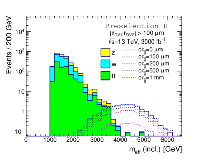
(a) $|\bm{r}_{\rm DV1}-\bm{r}_{\rm DV2}|>100~{}{\rm\mu m}$

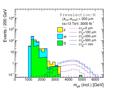
(b) $|\bm{r}_{\rm DV1}-\bm{r}_{\rm DV2}|>200~{}{\rm\mu m}$

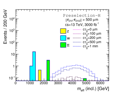
(c) $|\bm{r}_{\rm DV1}-\bm{r}_{\rm DV2}|>500~{}{\rm\mu m}$

Figure 8: Distributions of $m_{\rm eff}({\rm incl.})$ for the SM background and signal events with different values of $c\tau_{\tilde{g}}$. The masses of gluino and the LSP are set to be $2600$ GeV and $100$ GeV, respectively. We have imposed preselection-H and the vetoes given in Table 6.

In Tables 7 and 8, we present the expected number of background and signal events for an integrated luminosity of $\mathcal{L}=3000~{}{\rm fb}^{-1}$. In Table 7 (8), we consider the case of a light (heavy) LSP with $m_{\tilde{g}}=2800~{}(2400)$ GeV and $m_{\tilde{\chi_{1}^{0}}}=100~{}(1440)$ GeV, where preselection-H (-M) is used for the event preselection. We see that in both cases the new selection cut efficiently removes the SM background while maintaining a sizable amount of signal events for metastable gluinos. To see this more clearly, in Fig. 8, we show the distributions of $m_{\rm eff}({\rm incl.})$ for the SM background and signal events with different values of $c\tau_{\tilde{g}}$, with preselection-H and the vetoes in Table 6 imposed. The masses of gluino and the LSP are set to be $2600$ GeV and $100$ GeV, respectively. As seen in these plots, the new selection cut considerably reduces the SM background especially if we require a large separation between the reconstructed displaced vertices, which allows us to relax the cut on $m_{\rm eff}({\rm incl.})$ to keep a large number of signal events.

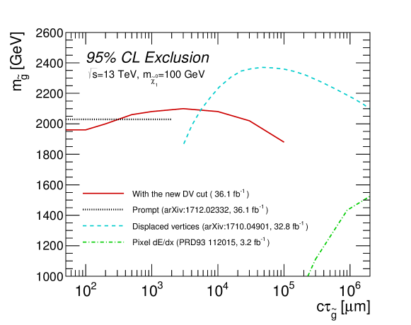
Figure 9: The 95% CL expected exclusion limit on the gluino mass with ${\cal L}=36.1\ {\rm fb}^{-1}$ at the 13 TeV LHC run as a function of $c\tau_{\tilde{g}}$ (red solid line). For comparison, we also show the 95% CL exclusion limits given by the ATLAS prompt-decay gluino search (black dotted line) [143], the ATLAS displaced-vertex search (blue dashed line) [66], and the ATLAS search of large ionization energy loss in the Pixel detector (green dot-dashed line) [72].

Now we show in Fig. 9 the expected limit on the gluino mass as a function of $c\tau_{\tilde{g}}$ based on the currently available luminosity of $36.1\ {\rm fb}^{-1}$ at the 13 TeV LHC (red solid line). Here the mass of LSP is set to be 100 GeV. The improvement in reach because of the new selection cut may be seen by comparing the reach for each $c\tau_{\tilde{g}}$ with that for $c\tau_{\tilde{g}}=0$, for which the new selection cut is ineffective as seen from Fig. 7(a). It turns out that, even with the current data, the exclusion limit can be improved by about $100$ and $120\ {\rm GeV}$ for $c\tau_{\tilde{g}}=0.5$ and $1\ {\rm mm}$, respectively. We also find that the sensitivity gets worse for $c\tau_{\tilde{g}}\gtrsim\mathcal{O}(10)$ mm. This is because the signal efficiency is decreased due to the requirements on the production point and impact parameters of tracks as well as the detector material veto on the position of reconstructed vertices. To compare the result with the current sensitivities of other gluino searches, we also show the 95% CL exclusion limits given by the ATLAS prompt-decay gluino search with the 13 TeV 36.1 fb^-1 data (black dotted line) [143], the ATLAS displaced-vertex search with the 13 TeV 32.8 fb^-1 data (blue dashed line) [66], and the ATLAS search of large ionization energy loss in the Pixel detector with the 13 TeV 3.2 fb^-1 data (green dot-dashed line) [72]. Note that we extend the black dotted line for the ATLAS prompt-decay gluino search up to $c\tau_{\tilde{g}}\sim\mathcal{O}(1)$ mm just for comparison; the reach of the prompt-decay gluino search is expected to become worse for $c\tau_{\tilde{g}}\gtrsim\mathcal{O}(1)$ mm [157]. We see that the existing metastable gluino searches are insensitive to a gluino with $c\tau_{\tilde{g}}\lesssim 1$ mm, where our event-selection criterion may offer a good sensitivity. In this sense, this new search strategy plays a complementary role in probing metastable gluinos.

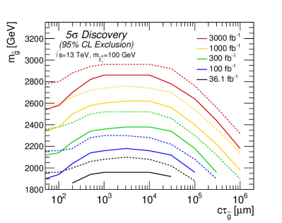
(a) $m_{\tilde{\chi}^{0}_{1}}=100$ GeV

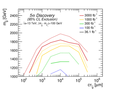
(b) $|m_{\tilde{g}}-m_{\tilde{\chi}^{0}_{1}}|=100$ GeV

Figure 10: The expected 95% CL exclusion limits (dotted) and $5\sigma$ discovery reaches (solid) as functions of $c\tau_{\tilde{g}}$ for different values of integrated luminosity at the 13 TeV LHC run.

In Fig. 10(a), we show the expected 95% CL exclusion limits (in dotted lines) and $5\sigma$ discovery reaches (in solid lines) for gluino as functions of $c\tau_{\tilde{g}}$ for different values of integrated luminosity at the 13 TeV LHC run, where the LSP mass is set to be 100 GeV. Notice that the expected reaches for an extremely small $c\tau_{\tilde{g}}$ should correspond to those for the prompt-decay gluino search with the same data set since the new selection cut plays no role in this case. As can be seen from this figure, the reach for the gluino can be extended with the help of the new selection cut for $c\tau_{\tilde{g}}\gtrsim 100~{}\mu{\rm m}$; e.g., for a gluino with $c\tau_{\tilde{g}}\sim\mathcal{O}$(1–10) mm, the expected discovery reach for the gluino mass can be extended by as large as $\sim 240$ GeV ($320$ GeV) with an integrated luminosity of ${\mathcal{L}}=300~{}{\rm fb}^{-1}$ (3000 fb^-1). These reaches for a gluino with $c\tau_{\tilde{g}}\sim\mathcal{O}$(1–10) mm are obtained with preselection H, $\left(m_{\rm effcut}\right)_{\rm optimal}=2400$ GeV ($3400$ GeV), and $\left(r_{\rm cut}\right)_{\rm optimal}\sim 300\,\mu{\rm m}$ ($160\,\mu{\rm m}$) for ${\mathcal{L}}=300\,{\rm fb}^{-1}$ ($3000\,{\rm fb}^{-1}$). Compared to a promptly decaying gluino, for which $\left(m_{\rm effcut}\right)_{\rm optimal}=3400$ GeV ($4200$ GeV), the $m_{\rm eff}({\rm incl.})$ selection cut is found to be significantly loosened, which implies that the new selection cut plays an important role in background rejection. As we already mentioned, because charged tracks with $|d_{0}|>10$ mm are not included in the analysis, and also because we reject all events in which a vertex is reconstructed with a position radius larger than $120$ mm, the expected exclusion limits decrease for $c\tau_{\tilde{g}}\gtrsim 100$ mm. Such a larger $c\tau_{\tilde{g}}$ region can however be covered by other long-lived gluino searches.

We also study the case where gluino and the LSP are degenerate in mass, which is motivated by the coannihilation scenario as we mentioned in Sec. 3. The result is shown in Fig. 10(b). Here, the mass difference between gluino and the LSP is set to be $100$ GeV. We find that the limits and the reaches are strongly enhanced especially for $c\tau_{\tilde{g}}\sim{\mathcal{O}}$(1–100) mm. Contrary to the previous case, we are unable to set a reach or limit higher than $1000$ GeV for low luminosities. A caveat here is that we impose relatively tight requirements on jet $p_{\rm T}$ and thus this analysis is not optimized for the degenerate mass region. Indeed, according to the analysis done by the ATLAS collaboration [160], the event selection category called Meff-5j-1400 provides the best sensitivity for the degenerate mass region, where conditions on $p_{\rm T}$ for 2nd–4th jets are relaxed and another 5th jet is required instead. We however do not try to further explore such an optimization in this paper—as the number of additional partons in our MC simulation is restricted to less than five—and defer it to another occasion.

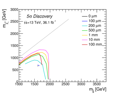
(a) $5\sigma$ discovery

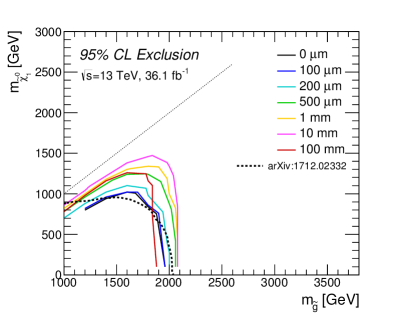
(b) Expected 95% CL exclusion

Figure 11: $5\sigma$ discovery reaches and expected 95% CL exclusion limits for gluinos with different $c\tau_{\tilde{g}}$, for an integrated luminosity of $36.1\,{\rm fb}^{-1}$. The expected 95% CL exclusion limit from the ATLAS promptly-decaying gluino search [143] is also shown in the black dotted line.

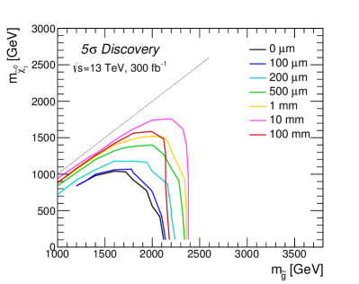
(a) $5\sigma$ discovery

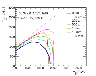
(b) Expected 95% CL exclusion

Figure 12: Same as in Fig. 11, but for an integrated luminosity of $300\,{\rm fb}^{-1}$.

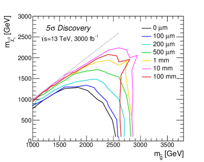
(a) $5\sigma$ discovery

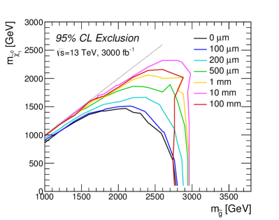
(b) Expected 95% CL exclusion

Figure 13: Same as in Fig. 11, but for an integrated luminosity of $3000\,{\rm fb}^{-1}$.

Finally, we present the $5\sigma$ discovery reaches and expected 95% CL exclusion limits for various values of $c\tau_{\tilde{g}}$ in Figs. 11, 12, and 13 for an integrated luminosity of 36.1, 300, and 3000 fb^-1, respectively. In Fig. 11(b), we also show the expected 95% CL exclusion limit given by the ATLAS experiment [143] in the black dotted line. We see that this ATLAS limit is in a fairly good agreement with our limit for $c\tau_{\tilde{g}}=0~{}{\rm\mu m}$ shown in the black solid line, besides the regions where gluino and the LSP are highly degenerate in mass. This discrepancy is expected since our analysis is not optimized for the degenerate region as we discussed above. From these plots, we see that an implementation of an extra cut utilizing the vertex reconstruction leads to a significant improvement in both the discovery reach and the exclusion limit for $c\tau_{\tilde{g}}\gtrsim 200\,\mu{\rm m}$. The extent of the improvement is maximized for $c\tau_{\tilde{g}}\sim{\mathcal{O}}$(1–10) mm and tends to get larger for a heavier LSP. This feature is also seen in Fig. 10, where we find that the improvement in the degenerate case (Fig. 10(b)) is much significant compared with the light LSP case (Fig. 10(a)). This follows from the fact that jets and the missing energy in gluino decays for the degenerate case tend to be soft, and thus traditional kinematical selection cuts become less powerful in this case. In such a situation, a sizable amount of the SM background remain after the kinematical selection cuts, but an additional cut based on vertex reconstruction can remove this efficiently, which results in a drastic improvement in the sensitivity.

4.4 Lifetime measurements

Once a new metastable particle is discovered at the LHC, the measurement of its lifetime is of crucial importance to understand the nature of new physics behind this metastable particle. For example, by measuring the lifetime of metastable gluino, we can infer the mass scale of squarks through Eq. (4). In this subsection, we discuss the prospects of the lifetime measurement by means of the displaced-vertex reconstruction.

To see this, we study the expected significance of rejection of a hypothesis that the gluino decay length is $c\tau_{\tilde{g}}^{\rm(hypo)}$ for gluino samples with a decay length of $c\tau_{\tilde{g}}$. Event samples are binned according to the distance between the two reconstructed vertices $|\bm{r}_{\rm DV1}-\bm{r}_{\rm DV2}|$ of the events. Then the expected significance $\langle Z_{c\tau_{\tilde{g}}^{\rm(hypo)}}\rangle_{c\tau_{\tilde{g}}}$ is defined by

$$\langle Z_{c\tau_{\tilde{g}}^{\rm(hypo)}}\rangle_{c\tau_{\tilde{g}}}\equiv\sqrt{\Delta\chi^{2}(c\tau_{\tilde{g}}^{\rm(hypo)},c\tau_{\tilde{g}})}~{},$$ (9)

where

$$\Delta\chi^{2}(c\tau_{\tilde{g}}^{\rm(hypo)},c\tau_{\tilde{g}})=\sum_{{\rm bin}\,\,i}\frac{\left\{S_{i}(c\tau_{\tilde{g}}^{\rm(hypo)})-S_{i}(c\tau_{\tilde{g}})\right\}^{2}}{S_{i}(c\tau_{\tilde{g}}^{\rm(hypo)})+B_{i}}\,.$$ (10)

Here, $S_{i}(c\tau)$ is the expected number of signal events in the bin $i$ on the assumption that gluinos have a decay length of $c\tau$, while $B_{i}$ is the number of SM background events.

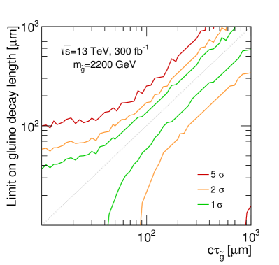
(a) ${\mathcal{L}}=300\,{\rm fb}^{-1}$

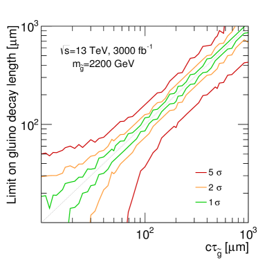
(b) ${\mathcal{L}}=3000\,{\rm fb}^{-1}$

Figure 14: The expected upper and lower bounds on the decay length of gluino as a function of the underlying value of $c\tau_{\tilde{g}}$. Here, we set $m_{\tilde{g}}=2.2$ TeV, and impose preselection-H and a selection cut $m_{\rm eff}({\rm incl.})>3500$ GeV.

In Figs. 14(a) and 14(b), we show the expected upper and lower bounds on the decay length as a function of $c\tau_{\tilde{g}}$ for a gluino with a mass of 2.2 TeV. Here we impose preselection-H and require $m_{\rm eff}({\rm incl.})>3500$ GeV. From these figures, we find that a metastable gluino with $c\tau_{\tilde{g}}\gtrsim 30~{}(60)~{}{\rm\mu m}$ can be distinguished from a promptly decaying one with the significance of $2\sigma$ ($5\sigma$) with an integrated luminosity of $3000~{}{\rm fb}^{-1}$. Moreover, Fig. 14(b) shows that the decay length of a gluino with $c\tau_{\tilde{g}}\sim{\cal O}(100)~{}\mu{\rm m}$ can be measured with an ${\cal O}(1)$ accuracy at the high-luminosity LHC. With such a measurement, we may probe the squark mass scale $m_{\tilde{q}}$ via Eq. (4) even though squarks are inaccessible at the LHC. We also note that even if only an upper limit on the gluino decay length is obtained, this gives valuable implications for SUSY models, since such a limit results in an upper bound on the squark mass scale; e.g., for $m_{\tilde{g}}=2.2$ TeV, an upper limit on the decay length $c\tau_{\tilde{g}}|_{\text{limit}}$ leads to

$$m_{\tilde{q}}\lesssim 10^{3}\times\biggl{(}\frac{c\tau_{\tilde{g}}|_{\text{limit}}}{100~{}\mu\text{m}}\biggr{)}^{\frac{1}{4}}~{}\text{TeV}~{}.$$ (11)

After all, the reconstruction of sub-millimeter decay vertices is quite important even after the discovery of a new particle such as gluino, as its lifetime contains precious information on the underlying physics.

5 100 TeV collider

The vertex-reconstruction method developed above can also be applied to other collider experiments. Recently, there have been a growing interest in future collider experiments with a center-of-mass energy higher than those at the LHC, such as a 100 TeV collider [78, 79]. Motivated by this, in this section we apply our new selection cut to the searches for metastable gluinos at a future $100$ TeV $pp$ collider and study how much this new selection cut can improve the sensitivity of the prompt-decay searches in this case. As we have already seen in Sec. 3, the production cross section of gluinos at a $100$ TeV collider is much larger than those at the LHC, which drastically extends the reach of gluino searches [78, 79, 153, 161]. In addition, particles tend to be produced in a highly boosted state at a 100 TeV collider, which then prolongs the lifetime of metastable particles—this allows us to probe particles with shorter decay length, as we actually see in the following analysis.

5.1 MC Simulation

$m_{\tilde{g}}$	$3,\,4,\,\ldots 6,\,8,\,\ldots 16,\,18$ TeV
$m_{\tilde{\chi}_{1}^{0}}$	$100$ GeV,
	$(0.2,\,0.4,\,0.6,\,0.8)\times m_{\tilde{g}}$,
	$m_{\tilde{g}}-(150\,{\rm GeV},\,100\,{\rm GeV},\,50\,{\rm GeV},\,25\,{\rm GeV})$
$c\tau_{\tilde{g}}$	$0,\,50,\,100,\,200,\,500,\,1000,\,3000$ ${\rm\mu m}$,
	$1\times 10^{4},\,3\times 10^{4},\,1\times 10^{5},\,3\times 10^{5},\,1\times 10^{6}$ ${\rm\mu m}$

Table 9: Sample points for signal events. We generate 50000 events for each sample point.

	bin $\alpha$	0	1	2	3	4
$H_{T,0}^{\rm max}(\alpha)$	(GeV)	$900$	$2100$	$4000$	$6400$	$\infty$
$\sigma_{\text{matched}}(\alpha)$	(pb)	$3.69{\scriptstyle\times 10^{2}}$	$25.8$	$2.30$	$0.23$	$0.04$
$N_{\text{matched}}(\alpha)$	$(\times 10^{3})$	$728$	$520$	$462$	$473$	$590$
$\mathcal{L}_{\rm gen}(\alpha)$	(${\rm ab}^{-1}$)	$1.97{\scriptstyle\times 10^{-3}}$	$0.0201$	$0.201$	$2.02$	$14.5$

(a) $Z\rightarrow\nu\bar{\nu}+0,1,2,3\,j$.

	bin $\alpha$	0	1	2	3	4
$H_{T,0}^{\rm max}(\alpha)$	(GeV)	$900$	$2100$	$4000$	$6400$	$\infty$
$\sigma_{\text{matched}}(\alpha)$	(pb)	$1.20{\scriptstyle\times 10^{3}}$	$22.4$	$1.70$	$0.16$	$0.03$
$N_{\text{matched}}(\alpha)$	$(\times 10^{3})$	$121$	$90.9$	$82.9$	$79.3$	$75.2$
$\mathcal{L}_{\rm gen}(\alpha)$	(${\rm ab}^{-1}$)	$1.01{\scriptstyle\times 10^{-4}}$	$4.06{\scriptstyle\times 10^{-3}}$	$0.0487$	$0.496$	$2.95$

(b) $Z\rightarrow\ell\bar{\ell}+0,1,2,3\,j$.

Table 10: The upper edge value of $H_{T,0}$, the leading-order matched cross section, the number of samples after matching, and equivalent luminosity in each $H_{T,0}$ bin for the $Z$-boson production process.

	bin $\alpha$	0	1	2	3	4	5
$H_{T,0}^{\rm max}(\alpha)$	(GeV)	$600$	$1500$	$3000$	$5000$	$7500$	$\infty$
$\sigma_{\text{matched}}(\alpha)$	(pb)	$9.62{\scriptstyle\times 10^{3}}$	$5.19{\scriptstyle\times 10^{2}}$	$41.7$	$3.93$	$0.49$	$0.09$
$N_{\text{matched}}(\alpha)$	$(\times 10^{3})$	$1910$	$1020$	$813$	$759$	$993$	$1950$
$\mathcal{L}_{\rm gen}(\alpha)$	(${\rm ab}^{-1}$)	$1.99{\scriptstyle\times 10^{-4}}$	$1.97{\scriptstyle\times 10^{-3}}$	$0.0195$	$0.193$	$2.05$	$20.6$

Table 11: Same as in Table 10 but for the $W$-boson production process.

	bin $\alpha$	0	1	2	3	4	5	6
$H_{T,0}^{\rm max}(\alpha)$	(GeV)	$800$	$1600$	$2800$	$4600$	$7200$	$10000$	$\infty$
$\sigma_{\text{matched}}(\alpha)$	(pb)	$4.40{\scriptstyle\times 10^{3}}$	$3.54{\scriptstyle\times 10^{2}}$	$33.7$	$3.40$	$0.34$	$0.03$	$5.18{\scriptstyle\times 10^{-3}}$
$N_{\text{matched}}(\alpha)$	$(\times 10^{3})$	$53.6$	$59.8$	$63.5$	$65.3$	$66.2$	$67.2$	$68$
$\mathcal{L}_{\rm gen}(\alpha)$	(${\rm ab}^{-1}$)	$1.22{\scriptstyle\times 10^{-5}}$	$1.69{\scriptstyle\times 10^{-4}}$	$1.89{\scriptstyle\times 10^{-3}}$	$0.0192$	$0.197$	$2.23$	$13.1$

(a) $t\bar{t}\rightarrow$ (semi-leptonic)$+0,1j$.

	bin $\alpha$	0	1	2	3	4
$H_{T,0}^{\rm max}(\alpha)$	(GeV)	$1100$	$2300$	$3900$	$6000$	$\infty$
$\sigma_{\text{matched}}(\alpha)$	(pb)	$54.4$	$6.57$	$0.56$	$0.06$	$6.90{\scriptstyle\times 10^{-3}}$
$N_{\text{matched}}(\alpha)$	$(\times 10^{3})$	$60.4$	$72.6$	$74.2$	$74.8$	$75.7$
$\mathcal{L}_{\rm gen}(\alpha)$	(${\rm ab}^{-1}$)	$1.11{\scriptstyle\times 10^{-3}}$	$1.11{\scriptstyle\times 10^{-2}}$	$0.133$	$1.36$	$11.0$

(b) $t\bar{t}\rightarrow$ (leptonic)$+0,1j$.

Table 12: Same as in Table 10 but for the $t\bar{t}$ production process.

For MC simulation of a 100 TeV collider, we basically follow the same procedure as described in Sec. 4.1. We list the sample points for signal events in Table 9, with the same categorization as in Table 1. We again generate 50000 events for each sample point. For the SM background processes, we again focus on the $Z$, $W$, and $t\bar{t}$ production processes, which turn out to be dominant [153]. We carry out simulations with up to three and one additional partons for the $Z/W$ and $t\bar{t}$ production processes, respectively. In generating background samples, we divide the generator-level phase space in terms of $H_{T,0}$; we show the binning of this division in Tables 10–12 for each process with the leading-order matched cross section, the number of samples after matching, and the equivalent luminosity.

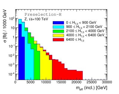
(a) $Z$ boson production

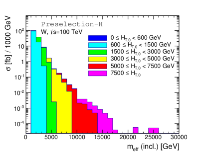
(b) $W$ boson production

Figure 15: Distributions of $m_{\text{eff}}(\text{incl.})$ with preselection-H required. Contributions from different $H_{T,0}$ bins are filled with different colors.

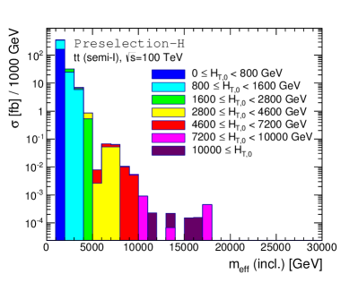
(a) Semi-leptonic $t\bar{t}$ decay

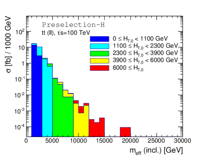
(b) Leptonic $t\bar{t}$ decay

Figure 16: Same as in Fig. 15, but for the $t\bar{t}$ production process.

Using these samples, we generate distributions of $m_{\rm eff}({\rm incl.})$ for each process with Preselection-H imposed. For reconstructed objects such as jets, charged leptons, and charged tracks, we use the same criteria as in Sec. 4.1. The resultant distributions are shown in Figs. 15 and 16. Again, we see a correlation between $H_{T,0}$ and $m_{\rm eff}({\rm incl.})$ and a sizable number of events in the tails, which justifies our way of dividing the phase space in terms of $H_{T,0}$.

To validate our MC simulation, we have compared the expected number of events obtained by our MC simulation with that given in Ref. [153], with the same selection cuts adopted there. We have found a fairly good agreement ($\sim 20\%$ level) with each other over the signal regions.

5.2 Event Selection

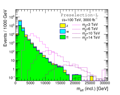
(a) Preselection-L

(b) Preselection-M

(c) Preselection-H

Figure 17: Distributions of $m_{\text{eff}}(\text{incl.})$ for the SM background and gluino signal events. We set the LSP mass to be 100 GeV.

For the preselection, we consider the same criteria as in Table 5. These criteria may be further optimized for a 100 TeV collider, but we do not discuss this possibility in this paper. We again impose the lepton and detector-material vetoes. In Fig. 17, we show the distributions of $m_{\rm eff}({\rm incl.})$ for the SM background and gluino signal events with each preselection imposed. We set the LSP mass to be 100 GeV in these plots.

(a) $m_{\tilde{g}}=3$ TeV

(b) $m_{\tilde{g}}=14$ TeV

Figure 18: The distributions of $|\bm{r}_{\rm DV1}-\bm{r}_{\rm DV2}|$ for a gluino with different values of $c\tau_{\tilde{g}}$, shown in the solid lines. The distributions for the SM background events are also shown in the dotted lines. We have imposed preselection-H, and $m_{\rm eff}({\rm incl.})>2800$ GeV (17600 GeV) in Fig. 18(a) (Fig. 18(b)).

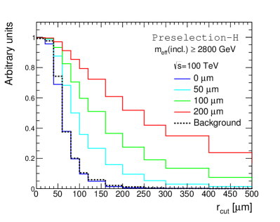
(a) $m_{\tilde{g}}=3$ TeV

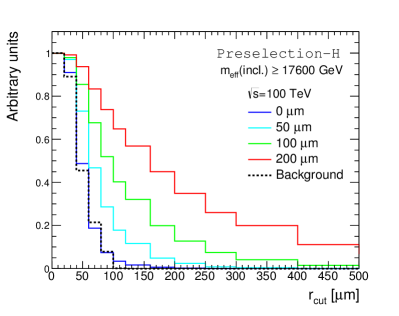
(b) $m_{\tilde{g}}=14$ TeV

Figure 19: Fractions of events which pass the selection cut $|\bm{r}_{\rm DV1}-\bm{r}_{\rm DV2}|>r_{\rm cut}$ for a gluino with different values of $c\tau_{\tilde{g}}$, shown in the solid lines. The distributions for the SM background events are also shown in the dotted lines. We have imposed preselection-H, and $m_{\rm eff}({\rm incl.})>2800$ GeV (17600 GeV) in Fig. 19(a) (Fig. 19(b)).

As we discuss in Sec. 2, the resolution of the vertex reconstruction highly depends on the track reconstruction performance of a detector. Due to a lack of concrete information on detectors at future 100 TeV colliders, in the following analysis, we just assume the same track-resolution parameters as those given in Sec. 4.2, and reconstruct vertices in the same manner as before. We show the distributions of $|\bm{r}_{\rm DV1}-\bm{r}_{\rm DV2}|$ in the solid lines for a gluino with different values of $c\tau_{\tilde{g}}$ and a mass of 3 TeV and 14 TeV in Figs. 18(a) and  18(b), respectively. Moreover, we show in Figs. 19(a) and 19(b) fractions of events which pass a selection cut of $|\bm{r}_{\rm DV1}-\bm{r}_{\rm DV2}|>r_{\rm cut}$ as functions of $r_{\rm cut}$. The distributions for the SM background events are also shown in the dotted lines. Here, we have imposed preselection-H, and $m_{\rm eff}({\rm incl.})>2800$ GeV (17600 GeV) in the left (right) panel. By comparing these figures with Fig. 6, we clearly see the effect of Lorentz boost of metastable particles on the displaced-vertex reconstruction. In Fig. 6, the distribution for the $c\tau_{\tilde{g}}=50~{}{\rm\mu m}$ case is found to be fairly close to those for $c\tau_{\tilde{g}}=0~{}{\rm\mu m}$ and the SM background. On the other hand, as seen in Figs. 18(a) and 19(a), we can easily distinguish $c\tau_{\tilde{g}}=50~{}{\rm\mu m}$ from $c\tau_{\tilde{g}}=0~{}{\rm\mu m}$ and the SM background at a 100 TeV collider. For a heavier gluino, however, the separation becomes less clear due to reduction in the boost factor.

5.3 Prospects

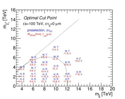
(a) $c\tau_{\tilde{g}}=0~{}{\rm\mu m}$

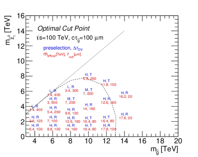
(b) $c\tau_{\tilde{g}}=100~{}{\rm\mu m}$

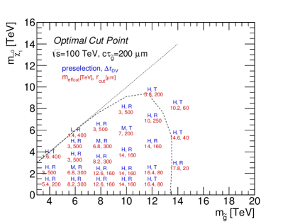
(c) $c\tau_{\tilde{g}}=200~{}{\rm\mu m}$

(d) $c\tau_{\tilde{g}}=500~{}{\rm\mu m}$

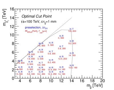
(e) $c\tau_{\tilde{g}}=1~{}{\rm mm}$

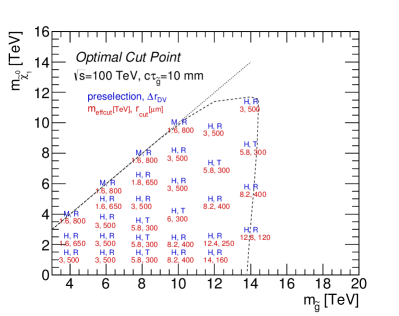
(f) $c\tau_{\tilde{g}}=10~{}{\rm mm}$

Figure 20: Optimal cut values ($(m_{\rm effcut})_{\rm optimal}$, $(r_{\rm cut})_{\rm optimal}$), the preselection (L, M, H), and the discriminator $\Delta r_{\rm DV}$ (R, T, Z) for each sample point with various $c\tau_{\tilde{g}}$, with an integrated luminosity of $3000~{}{\rm fb}^{-1}$. The expected $5\sigma$ discovery reaches for gluinos are also shown in the dashed lines.

	$Z$	$W$	$t\bar{t}$	total
preselection-H  $(\times 10^{6})$	$0.42{\scriptstyle~{}\pm 0.01}$	$0.45{\scriptstyle~{}\pm 0.02}$	$1.26{\scriptstyle~{}\pm 0.4}$	$2.13{\scriptstyle~{}\pm 0.4}$
$m_{\rm eff}({\rm incl.})>17.8$ TeV	$3.1{\scriptstyle~{}\pm 0.8}$	$0.9{\scriptstyle~{}\pm 0.3}$	$0.5{\scriptstyle~{}\pm 0.4}$	$4.6{\scriptstyle~{}\pm 0.9}$
$\bigl{|}\bm{r}_{\rm DV1}-\bm{r}_{\rm DV2}\bigr{|}>100~{}{\rm\mu m}$	$<0.1$	$<0.1$	$<0.1$	$<0.1$
$\bigl{|}\bm{r}_{\rm DV1}-\bm{r}_{\rm DV2}\bigr{|}>200~{}{\rm\mu m}$	$<0.1$	$<0.1$	$<0.1$	$<0.1$

(a) The expected number of background events.

	$c\tau_{\tilde{g}}=0$	$c\tau_{\tilde{g}}=200~{}{\rm\mu m}$	$c\tau_{\tilde{g}}=500~{}{\rm\mu m}$	$c\tau_{\tilde{g}}=1~{}{\rm mm}$
preselection-H	$20.5{\scriptstyle~{}\pm 0.3}$
$m_{\rm eff}({\rm incl.})>17.8$ TeV	$14.5{\scriptstyle~{}\pm 0.2}$
$\bigl{|}\bm{r}_{\rm DV1}-\bm{r}_{\rm DV2}\bigr{|}>100~{}{\rm\mu m}$	$0.5{\scriptstyle~{}\pm 0.04}$	$9.8{\scriptstyle~{}\pm 0.2}$	$12.5{\scriptstyle~{}\pm 0.2}$	$12.9{\scriptstyle~{}\pm 0.2}$
$\bigl{|}\bm{r}_{\rm DV1}-\bm{r}_{\rm DV2}\bigr{|}>200~{}{\rm\mu m}$	$<0.1$	$5.5{\scriptstyle~{}\pm 0.1}$	$9.6{\scriptstyle~{}\pm 0.2}$	$11.3{\scriptstyle~{}\pm 0.2}$

(b) The expected number of signal events for $m_{\tilde{g}}=12$ TeV, $m_{\tilde{\chi}_{1}^{0}}=100$ GeV with different values of $c\tau_{\tilde{g}}$.

Table 13: The expected number of background (a) and signal (b) events for an integrated luminosity of $\mathcal{L}=3000~{}{\rm fb}^{-1}$. We set the masses of gluino and the LSP to be $12$ TeV and $100$ GeV, respectively.

	$Z$	$W$	$t\bar{t}$	total
preselection-H  $(\times 10^{6})$	$0.42{\scriptstyle~{}\pm 0.01}$	$0.45{\scriptstyle~{}\pm 0.02}$	$1.26{\scriptstyle~{}\pm 0.4}$	$2.13{\scriptstyle~{}\pm 0.4}$
$m_{\rm eff}({\rm incl.})>6$ TeV  $(\times 10^{3})$	$2.2{\scriptstyle~{}\pm 0.1}$	$1.0{\scriptstyle~{}\pm 0.1}$	$0.8{\scriptstyle~{}\pm 0.2}$	$4.0{\scriptstyle~{}\pm 0.3}$
$\bigl{|}\bm{r}_{\rm DV1}-\bm{r}_{\rm DV2}\bigr{|}>200~{}{\rm\mu m}$	$5.9{\scriptstyle~{}\pm 3}$	$5.7{\scriptstyle~{}\pm 2.}$	$2.2{\scriptstyle~{}\pm 2}$	$14{\scriptstyle~{}\pm 4}$
$\bigl{|}\bm{r}_{\rm DV1}-\bm{r}_{\rm DV2}\bigr{|}>500~{}{\rm\mu m}$	$<0.1$	$<0.1$	$<0.1$	$<0.1$

(a) The expected number of background events.

	$c\tau_{\tilde{g}}=0$	$c\tau_{\tilde{g}}=200~{}{\rm\mu m}$	$c\tau_{\tilde{g}}=500~{}{\rm\mu m}$	$c\tau_{\tilde{g}}=1~{}{\rm mm}$
preselection-H	$143{\scriptstyle~{}\pm 2}$
$m_{\rm eff}({\rm incl.})>6$ TeV	$70{\scriptstyle~{}\pm 1}$
$\bigl{|}\bm{r}_{\rm DV1}-\bm{r}_{\rm DV2}\bigr{|}>200~{}{\rm\mu m}$	$0.4{\scriptstyle~{}\pm 0.1}$	$26.5{\scriptstyle~{}\pm 0.7}$	$45.1{\scriptstyle~{}\pm 0.9}$	$53.5{\scriptstyle~{}\pm 1}$
$\bigl{|}\bm{r}_{\rm DV1}-\bm{r}_{\rm DV2}\bigr{|}>500~{}{\rm\mu m}$	$<0.1$	$6.4{\scriptstyle~{}\pm 0.3}$	$22.8{\scriptstyle~{}\pm 0.6}$	$36.5{\scriptstyle~{}\pm 0.8}$

(b) The expected number of signal events for $m_{\tilde{g}}=10$ TeV, $m_{\tilde{\chi}_{1}^{0}}=8$ TeV with different values of $c\tau_{\tilde{g}}$.

Table 14: Same as Table. 13 but the masses of gluino and the LSP are set to be $10$ TeV and $8$ TeV, respectively.

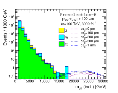
(a) $|\bm{r}_{\rm DV1}-\bm{r}_{\rm DV2}|>100~{}{\rm\mu m}$

(b) $|\bm{r}_{\rm DV1}-\bm{r}_{\rm DV2}|>200~{}{\rm\mu m}$

(c) $|\bm{r}_{\rm DV1}-\bm{r}_{\rm DV2}|>500~{}{\rm\mu m}$

Figure 21: Distributions of $m_{\rm eff}({\rm incl.})$ for the SM background and signal events with different values of $c\tau_{\tilde{g}}$. The masses of gluino and the LSP are set to be $14$ TeV and $100$ GeV, respectively. We have imposed preselection-H and the vetoes given in Table 6.

Now we discuss the prospects of our new selection cut for a 100 TeV collider. We again use the event selection criteria summarized in Table 6, except that we now raise the upper limit on $m_{\rm effcut}$ to $3\times 10^{4}$ GeV. In Fig. 20, we show optimal cut values ($(m_{\rm effcut})_{\rm optimal}$, $(r_{\rm cut})_{\rm optimal}$), the preselection (L, M, or H), and the discriminator $\Delta r_{\rm DV}$ (R, T, or Z) for each sample point with various $c\tau_{\tilde{g}}$, for a 100 TeV collider with an integrated luminosity of $3000~{}{\rm fb}^{-1}$. The expected $5\sigma$ discovery reaches for gluinos are also shown in the dashed lines. We again find that the kinematic selection cut on $m_{\rm eff}({\rm incl.})$ may be highly relaxed with the help of the displaced-vertex cut with $(r_{\rm cut})_{\rm optimal}\simeq c\tau_{\tilde{g}}$. In Tables 13 and 14, we present the expected number of background and signal events for an integrated luminosity of $\mathcal{L}=3000~{}{\rm fb}^{-1}$. In Table 13 (14), we consider the case of a light (heavy) LSP with $m_{\tilde{g}}=12~{}(10)$ TeV and $m_{\tilde{\chi_{1}^{0}}}=100$ GeV (8 TeV). We then show the distributions of $m_{\rm eff}({\rm incl.})$ for the SM background and signal events with different values of $c\tau_{\tilde{g}}$ in Fig. 21, with preselection-H and the vetoes in Table 6 imposed. The masses of gluino and the LSP are set to be $14$ TeV and $100$ GeV, respectively. Both the tables and figures demonstrate that also at a 100 TeV collider our displaced-vertex selection cut can efficiently eliminate the SM background while keeping the signal events.

(a) $m_{\tilde{\chi}^{0}_{1}}=100$ GeV

(b) $|m_{\tilde{g}}-m_{\tilde{\chi}^{0}_{1}}|=100$ GeV

Figure 22: The expected 95% CL exclusion limits (dotted) and $5\sigma$ discovery reaches (solid) as functions of $c\tau_{\tilde{g}}$ for different values of integrated luminosity at a future 100 TeV $pp$ collider. The expected exclusion limit (discovery reach) for $c\tau_{\tilde{g}}=0$ is represented by a circle (a blob).

In Fig. 22(a), we show the expected 95% CL exclusion limits (in dotted lines) and $5\sigma$ discovery reaches (in solid lines) for gluino as functions of $c\tau_{\tilde{g}}$ for different values of integrated luminosity at a 100 TeV collider, where the LSP mass is set to be 100 GeV. The expected exclusion limit (discovery reach) for $c\tau_{\tilde{g}}=0$ is represented by a circle (a blob). As can be seen from the figure, the reach for the gluino can be extended with the help of the additional displaced-vertex cut for $c\tau_{\tilde{g}}\gtrsim 100~{}\mu{\rm m}$; for instance, for a gluino with $c\tau_{\tilde{g}}\sim\mathcal{O}$(1–10) mm, the expected discovery reach for the gluino mass can be extended by as large as $\sim 1.4$ TeV ($1.8$ TeV) with an integrated luminosity of ${\mathcal{L}}=300~{}{\rm fb}^{-1}$ (3000 fb^-1). These reaches for a gluino with $c\tau_{\tilde{g}}\sim\mathcal{O}$(1–10) mm are obtained with preselection-H, $|\bm{r}_{\rm DV1}-\bm{r}_{\rm DV2}|$  ($|\bm{r}_{\rm DV1}-\bm{r}_{\rm DV2}|_{\rm T}$) with $(m_{\rm effcut})_{\rm optimal}=10$ TeV ($12.6$ TeV), and $(r_{\rm cut})_{\rm optimal}\sim 120\,\mu{\rm m}$ ($160\,\mu{\rm m}$) for ${\mathcal{L}}=300\,{\rm fb}^{-1}$ ($3000\,{\rm fb}^{-1}$). Compared to a promptly decaying gluino, where the optimized values for $(m_{\rm effcut})_{\rm optimal}$ are given by 13.8 TeV and $17.8$ TeV for ${\mathcal{L}}=300~{}{\rm fb}^{-1}$ and 3000 fb^-1, respectively, the $m_{\rm eff}({\rm incl.})$ selection cut is loosened and the new vertex-based selection cut is responsible for the reduction of background. We also show the degenerate case in Fig. 22(b), where the mass difference between gluino and the LSP is set to be $100$ GeV. We see a drastic enhancement in reaches, especially for $c\tau_{\tilde{g}}\sim{\mathcal{O}}$(1–100) mm.

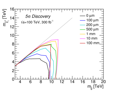
(a) $5\sigma$ discovery

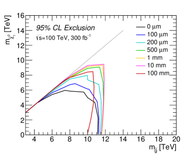
(b) Expected 95% CL exclusion

Figure 23: $5\sigma$ discovery reaches and expected 95% CL exclusion limits for gluinos with different $c\tau_{\tilde{g}}$, for an integrated luminosity of $300\,{\rm fb}^{-1}$.

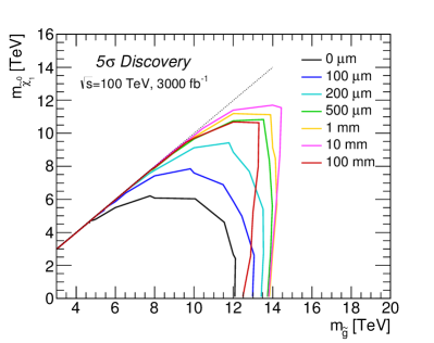
(a) $5\sigma$ discovery

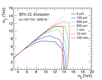
(b) Expected 95% CL exclusion

Figure 24: Same as in Fig. 23, but for an integrated luminosity of $3000\,{\rm fb}^{-1}$.

Finally, we show the $5\sigma$ discovery reaches and expected 95% CL exclusion limits for various values of $c\tau_{\tilde{g}}$ in Figs. 23 and 24 for an integrated luminosity of 300 and 3000 fb^-1, respectively. These figures illustrate that the use of our vertex-based selection cut leads to a significant improvement in both the discovery reach and the exclusion limit for $c\tau_{\tilde{g}}\gtrsim 100\,\mu{\rm m}$. Notice that, compared with the 13 TeV case, searches at a 100 TeV collider may be sensitive to gluinos with a shorter lifetime. The extent of the improvement is maximized for $c\tau_{\tilde{g}}\sim{\mathcal{O}}$(1–10) mm and tends to get larger for a heavier LSP, similarly to the 13 TeV LHC case. We also find a dramatic improvement in the degenerate mass region; with the displaced-vertex selection cut, we may probe a gluino degenerate with the LSP in mass up to $\sim 10$ TeV. This has significant implications for the gluino coannihilation scenario, given that an upper limit on the gluino mass is set for this scenario as $m_{\tilde{g}}\lesssim 8$ TeV [135]. Our analysis indicates that we may probe the whole range of the gluino coannihilation scenario at a 100 TeV collider if the gluino decay length falls into the range of $100~{}\mu\text{m}\lesssim c\tau_{\tilde{g}}\lesssim 100~{}\text{mm}$.

6 Conclusion and discussion

In this paper we have discussed a strategy of improving searches for metastable particles at hadron colliders. This strategy is based on the reconstruction of displaced vertices caused by the decay of metastable particles. We take account of this information as a new event-selection cut and impose this in addition to the conventional selection criteria based on kinematical observables. To see the significance of this new selection cut, we consider metastable gluinos in SUSY models as an example, whose decay length falls into the sub-millimeter range if squark masses are around the PeV scale. Then, we have studied the implications of this new selection cut for the gluino searches at both the 13 TeV LHC and future 100 TeV $pp$ collider experiments. We have performed MC simulations for both the signal and SM background events, and take into account the effect of the track reconstruction performance on the resolution of vertex reconstruction. We have also discussed optimization of kinematical selection criteria in the presence of the new vertex selection cut. As it turns out, we can considerably relax the kinematical selection criteria in this case, which is of great importance especially for the cases where gluino and the LSP are degenerate in mass.

For the 13 TeV LHC analysis, we have found that our vertex-reconstruction method can separate out decay vertices if the gluino decay length is $\gtrsim 100~{}\mu{\rm m}$. As a result, with the displaced-vertex cut, we may considerably improve the potential of gluino searches for a gluino with $c\tau_{\tilde{g}}\gtrsim 200~{}\mu{\rm m}$. In particular, if $c\tau_{\tilde{g}}\sim\mathcal{O}$(1–10) mm, then the exclusion and discovery reaches for the gluino mass can be extended by about $180$ GeV and $320$ GeV, respectively, with an integrated luminosity of 3000 fb^-1 at the 13 TeV LHC for LSP with a mass of $100$ GeV. This improvement gets more drastic when gluino and the LSP are degenerate in mass. Furthermore, with an integrated luminosity of 3000 fb^-1, it is possible to measure the gluino decay length with an ${\cal O}(1)$ accuracy for a gluino with $c\tau_{\tilde{g}}\sim{\cal O}(100)~{}\mu{\rm m}$ and $m_{\tilde{g}}=2.2$ TeV, which may allow us to probe the PeV-scale squarks indirectly.

After the discovery of a metastable particle, its lifetime information will become available by trying to reconstruct displaced vertices as we have seen in Sec. 4.4. In the case of gluino, such information can be used to constrain the mass scale of squarks which mediate the decay processes. Even though we can only have an upper bound on the lifetime if the decay length $c\tau_{\tilde{g}}$ is shorter than $\sim 100~{}\mu{\rm m}$, such an bound is highly useful because it can provide an upper bound on the mass scale of squarks whose direct production may not be possible at the LHC. For the gluino mass of $2.2\ {\rm TeV}$, for example, the mass scale of the squarks will be known to be lower than the PeV scale or a longevity of gluino will be observed.

We have also studied the prospects of searches for metastable gluinos at a future $100$ TeV $pp$ collider. Since the TeV-scale gluinos tend to be produced in a fairly boosted state at a 100 TeV collider, we expect it is possible to probe a shorter decay length compared with the LHC case. Indeed, we have found that the $|\bm{r}_{\rm DV1}-\bm{r}_{\rm DV2}|$ distributions for a 3 TeV gluino are quite different from those for the $c\tau_{\tilde{g}}=0$ case if its decay distance is $\gtrsim 50~{}{\rm\mu m}$. By using the new selection cut, we can significantly extend the exclusion limits and discovery reaches of gluino searches for $c\tau_{\tilde{g}}\gtrsim 100~{}\mu{\rm m}$; e.g., for $c\tau_{\tilde{g}}\sim\mathcal{O}$(1–10) mm, the exclusion and discovery reaches of gluino mass will be extended by about $780$ GeV and $1780$ GeV, respectively, with an integrated luminosity of 3000 fb^-1 and the LSP mass being $100$ GeV. The improvement is found to be more drastic in the degenerate mass region.

In the analyses given in this paper, we have assumed that gluinos decay into only the first-generation quarks and a LSP. In reality, the dominant decay channel of a gluino depends on the mass spectrum of squarks; for instance, if stops are much lighter than the other squarks, then the $\tilde{g}\rightarrow t\bar{t}\tilde{\chi}_{1}^{0}$ decay process becomes the dominant decay channel. In this case, besides the displaced vertices associated with the gluino decay, we may also find the secondary vertices that originate from long-lived hadrons including $b$ quarks, which are emitted by top quarks in the final state. Moreover, if there is a sizable flavor violation in the sfermion mass matrices—this possibility is experimentally allowed if the mass scale of SUSY particles lies around the PeV scale as we discussed in Sec. 3—the decay of gluinos may exhibit this flavor mixing by containing quarks with different flavors in the final state [162]. Secondary vertices due to metastable hadrons may also appear in such cases. The presence of secondary vertices may affect the resolution of the vertex reconstruction, whereas this distinct signature composed of multiple displaced vertices may allow further optimization for this class of decay processes. A dedicated study regarding this possibility may be worth doing.

Another possibility of optimization is related to the degenerate mass region. As we observed in Fig. 11(b) in Sec. 4.3, the limits we obtained in the degenerate mass region are weaker than that presented in Ref. [143], since our analysis was not optimized to the degenerate mass region. Such an optimization is however possible by relaxing the requirements on the jet momenta. In fact, this is quite promising given that our new selection cut can significantly reduce the SM background and thus allow a relaxation of kinematical selection criteria as we have seen in the above analyses. This expectation is actually supported by the recent ATLAS result of the displaced-vertex search [66], where an optimization for the degenerate mass region was successfully carried out and a stringent limit is imposed on long-lived gluinos in a degenerate mass spectrum.

In this analysis, we do not reconstruct the position of the primary interaction point and use only the distance of the two displaced vertices as a discriminator. As we mentioned in Sec. 4.2, however, the reconstruction of the primary vertex may also be possible by using the remnants of the $pp$ collision and/or initial state radiation emitted from the vertex. This additional information could be useful for the further reduction of background events. For instance, by requiring the presence of the primary vertex in-between the two reconstructed vertices we may efficiently reject the SM background contribution. Another, in fact simpler way of going beyond the mere use of the vertex distance is to require both of the two decay vertices to be reconstructed away from the beam line, with which we can avoid the misidintification of the primary vertex as one of the two decay vertices. Such elaboration of our new selection cut will be explored in another occasion.

Finally we comment here that, by reconstructing the positions of displaced vertices as well as the momenta of the charged tracks associated with these vertices, we may also extract the kinematical information of both the decaying and final-state invisible particles, as discussed in Refs. [163, 164]. In particular, we may determine the masses of these particles from the above information. This technique may be useful not only for studying the mass spectrum of the decay chain after the discovery of the metastable particle, but also for an additional event-selection cut to reduce the SM background. A dedicated study is required to assess the feasibility of this method, and thus we defer it to future work.

References

- [1] M. Fairbairn, A. C. Kraan, D. A. Milstead, T. Sjostrand, P. Z. Skands, and T. Sloan, Stable massive particles at colliders, Phys. Rept. 438 (2007) 1–63, [hep-ph/0611040].
- [2] M. Toharia and J. D. Wells, Gluino decays with heavier scalar superpartners, JHEP 02 (2006) 015, [hep-ph/0503175].
- [3] P. Gambino, G. F. Giudice, and P. Slavich, Gluino decays in split supersymmetry, Nucl. Phys. B726 (2005) 35–52, [hep-ph/0506214].
- [4] R. Sato, S. Shirai, and K. Tobioka, Gluino Decay as a Probe of High Scale Supersymmetry Breaking, JHEP 11 (2012) 041, [arXiv:1207.3608].
- [5] G. F. Giudice and R. Rattazzi, Theories with gauge mediated supersymmetry breaking, Phys. Rept. 322 (1999) 419–499, [hep-ph/9801271].
- [6] P. Draper, P. Meade, M. Reece, and D. Shih, Implications of a 125 GeV Higgs for the MSSM and Low-Scale SUSY Breaking, Phys. Rev. D85 (2012) 095007, [arXiv:1112.3068].
- [7] J. A. Evans and J. Shelton, Long-Lived Staus and Displaced Leptons at the LHC, JHEP 04 (2016) 056, [arXiv:1601.01326].
- [8] B. C. Allanach, M. Badziak, G. Cottin, N. Desai, C. Hugonie, and R. Ziegler, Prompt Signals and Displaced Vertices in Sparticle Searches for Next-to-Minimal Gauge Mediated Supersymmetric Models, Eur. Phys. J. C76 (2016), no. 9 482, [arXiv:1606.03099].
- [9] R. Barbier et al., R-parity violating supersymmetry, Phys. Rept. 420 (2005) 1–202, [hep-ph/0406039].
- [10] P. W. Graham, D. E. Kaplan, S. Rajendran, and P. Saraswat, Displaced Supersymmetry, JHEP 07 (2012) 149, [arXiv:1204.6038].
- [11] P. Ghosh, I. Lara, D. E. Lopez-Fogliani, C. Munoz, and R. Ruiz de Austri, Searching for left sneutrino LSP at the LHC, arXiv:1707.02471.
- [12] A. Brandenburg, L. Covi, K. Hamaguchi, L. Roszkowski, and F. D. Steffen, Signatures of axinos and gravitinos at colliders, Phys. Lett. B617 (2005) 99–111, [hep-ph/0501287].
- [13] K. Hamaguchi, M. M. Nojiri, and A. de Roeck, Prospects to study a long-lived charged next lightest supersymmetric particle at the LHC, JHEP 03 (2007) 046, [hep-ph/0612060].
- [14] A. Freitas, F. D. Steffen, N. Tajuddin, and D. Wyler, Axinos in Cosmology and at Colliders, JHEP 06 (2011) 036, [arXiv:1105.1113].
- [15] G. Barenboim, E. J. Chun, S. Jung, and W. I. Park, Implications of an axino LSP for naturalness, Phys. Rev. D90 (2014), no. 3 035020, [arXiv:1407.1218].
- [16] C. S. Redino and D. Wackeroth, Exploring the Hadronic Axion Window via Delayed Neutralino Decay to Axinos at the LHC, Phys. Rev. D93 (2016), no. 7 075022, [arXiv:1512.06822].
- [17] R. T. Co, F. D’Eramo, and L. J. Hall, Gravitino or Axino Dark Matter with Reheat Temperature as high as GeV, JHEP 03 (2017) 005, [arXiv:1611.05028].
- [18] R. T. Co, F. D’Eramo, L. J. Hall, and K. Harigaya, Saxion Cosmology for Thermalized Gravitino Dark Matter, JHEP 07 (2017) 125, [arXiv:1703.09796].
- [19] J. Fan, M. Reece, and J. T. Ruderman, Stealth Supersymmetry, JHEP 11 (2011) 012, [arXiv:1105.5135].
- [20] J. Fan, M. Reece, and J. T. Ruderman, A Stealth Supersymmetry Sampler, JHEP 07 (2012) 196, [arXiv:1201.4875].
- [21] J. Fan, R. Krall, D. Pinner, M. Reece, and J. T. Ruderman, Stealth Supersymmetry Simplified, JHEP 07 (2016) 016, [arXiv:1512.05781].
- [22] B. Batell, G. F. Giudice, and M. McCullough, Natural Heavy Supersymmetry, JHEP 12 (2015) 162, [arXiv:1509.00834].
- [23] J. L. Evans, T. Gherghetta, N. Nagata, and Z. Thomas, Naturalizing Supersymmetry with a Two-Field Relaxion Mechanism, JHEP 09 (2016) 150, [arXiv:1602.04812].
- [24] J. L. Feng, T. Moroi, L. Randall, M. Strassler, and S.-f. Su, Discovering supersymmetry at the Tevatron in wino LSP scenarios, Phys. Rev. Lett. 83 (1999) 1731–1734, [hep-ph/9904250].
- [25] M. Ibe, T. Moroi, and T. T. Yanagida, Possible Signals of Wino LSP at the Large Hadron Collider, Phys. Lett. B644 (2007) 355–360, [hep-ph/0610277].
- [26] S. Asai, T. Moroi, K. Nishihara, and T. T. Yanagida, Testing the Anomaly Mediation at the LHC, Phys. Lett. B653 (2007) 81–87, [arXiv:0705.3086].
- [27] S. Asai, T. Moroi, and T. T. Yanagida, Test of Anomaly Mediation at the LHC, Phys. Lett. B664 (2008) 185–189, [arXiv:0802.3725].
- [28] S. Asai, Y. Azuma, O. Jinnouchi, T. Moroi, S. Shirai, and T. T. Yanagida, Mass Measurement of the Decaying Bino at the LHC, Phys. Lett. B672 (2009) 339–343, [arXiv:0807.4987].
- [29] Z. Liu and B. Tweedie, The Fate of Long-Lived Superparticles with Hadronic Decays after LHC Run 1, JHEP 06 (2015) 042, [arXiv:1503.05923].
- [30] N. Nagata, H. Otono, and S. Shirai, Probing bino-gluino coannihilation at the LHC, Phys. Lett. B748 (2015) 24–29, [arXiv:1504.00504].
- [31] N. Nagata, H. Otono, and S. Shirai, Probing Bino-Wino Coannihilation at the LHC, JHEP 10 (2015) 086, [arXiv:1506.08206].
- [32] K. Rolbiecki and K. Sakurai, Long-lived bino and wino in supersymmetry with heavy scalars and higgsinos, JHEP 11 (2015) 091, [arXiv:1506.08799].
- [33] N. Nagata, H. Otono, and S. Shirai, Cornering Compressed Gluino at the LHC, JHEP 03 (2017) 025, [arXiv:1701.07664].
- [34] H. Fukuda, N. Nagata, H. Otono, and S. Shirai, Higgsino Dark Matter or Not: Role of Disappearing Track Searches at the LHC and Future Colliders, arXiv:1703.09675.
- [35] Z. Chacko, H.-S. Goh, and R. Harnik, The Twin Higgs: Natural electroweak breaking from mirror symmetry, Phys. Rev. Lett. 96 (2006) 231802, [hep-ph/0506256].
- [36] G. Burdman, Z. Chacko, H.-S. Goh, and R. Harnik, Folded supersymmetry and the LEP paradox, JHEP 02 (2007) 009, [hep-ph/0609152].
- [37] H. Cai, H.-C. Cheng, and J. Terning, A Quirky Little Higgs Model, JHEP 05 (2009) 045, [arXiv:0812.0843].
- [38] G. Burdman and R. T. D’Agnolo, Scalar Leptons in Folded Supersymmetry, arXiv:1512.00040.
- [39] Z. Chacko, D. Curtin, and C. B. Verhaaren, A Quirky Probe of Neutral Naturalness, Phys. Rev. D94 (2016), no. 1 011504, [arXiv:1512.05782].
- [40] M. J. Strassler and K. M. Zurek, Echoes of a hidden valley at hadron colliders, Phys. Lett. B651 (2007) 374–379, [hep-ph/0604261].
- [41] M. J. Strassler and K. M. Zurek, Discovering the Higgs through highly-displaced vertices, Phys. Lett. B661 (2008) 263–267, [hep-ph/0605193].
- [42] M. J. Strassler, Possible effects of a hidden valley on supersymmetric phenomenology, hep-ph/0607160.
- [43] Y. Nakai, M. Reece, and R. Sato, SUSY Higgs Mass and Collider Signals with a Hidden Valley, JHEP 03 (2016) 143, [arXiv:1511.00691].
- [44] S. Knapen, H. K. Lou, M. Papucci, and J. Setford, Tracking down Quirks at the Large Hadron Collider, Phys. Rev. D96 (2017), no. 11 115015, [arXiv:1708.02243].
- [45] J. Barnard, P. Cox, T. Gherghetta, and A. Spray, Long-Lived, Colour-Triplet Scalars from Unnaturalness, JHEP 03 (2016) 003, [arXiv:1510.06405].
- [46] S. Chang and M. A. Luty, Displaced Dark Matter at Colliders, arXiv:0906.5013.
- [47] R. T. Co, F. D’Eramo, L. J. Hall, and D. Pappadopulo, Freeze-In Dark Matter with Displaced Signatures at Colliders, JCAP 1512 (2015), no. 12 024, [arXiv:1506.07532].
- [48] O. Buchmueller, A. De Roeck, K. Hahn, M. McCullough, P. Schwaller, K. Sung, and T.-T. Yu, Simplified Models for Displaced Dark Matter Signatures, JHEP 09 (2017) 076, [arXiv:1704.06515].
- [49] B. S. Acharya, S. A. R. Ellis, G. L. Kane, B. D. Nelson, and M. Perry, Categorisation and Detection of Dark Matter Candidates from String/M-theory Hidden Sectors, arXiv:1707.04530.
- [50] L. Basso, A. Belyaev, S. Moretti, and C. H. Shepherd-Themistocleous, Phenomenology of the minimal B-L extension of the Standard model: Z’ and neutrinos, Phys. Rev. D80 (2009) 055030, [arXiv:0812.4313].
- [51] J. C. Helo, M. Hirsch, and S. Kovalenko, Heavy neutrino searches at the LHC with displaced vertices, Phys. Rev. D89 (2014) 073005, [arXiv:1312.2900]. [Erratum: Phys. Rev.D93,no.9,099902(2016)].
- [52] E. Izaguirre and B. Shuve, Multilepton and Lepton Jet Probes of Sub-Weak-Scale Right-Handed Neutrinos, Phys. Rev. D91 (2015), no. 9 093010, [arXiv:1504.02470].
- [53] A. Maiezza, M. Nemevšek, and F. Nesti, Lepton Number Violation in Higgs Decay at LHC, Phys. Rev. Lett. 115 (2015) 081802, [arXiv:1503.06834].
- [54] S. Antusch, E. Cazzato, and O. Fischer, Displaced vertex searches for sterile neutrinos at future lepton colliders, JHEP 12 (2016) 007, [arXiv:1604.02420].
- [55] S. Antusch, E. Cazzato, and O. Fischer, Sterile neutrino searches at future , , and colliders, Int. J. Mod. Phys. A32 (2017), no. 14 1750078, [arXiv:1612.02728].
- [56] E. Accomando, L. Delle Rose, S. Moretti, E. Olaiya, and C. H. Shepherd-Themistocleous, Novel SM-like Higgs decay into displaced heavy neutrino pairs in U(1)′ models, JHEP 04 (2017) 081, [arXiv:1612.05977].
- [57] M. Nemevšek, F. Nesti, and J. C. Vasquez, Majorana Higgses at colliders, JHEP 04 (2017) 114, [arXiv:1612.06840].
- [58] P. Bhupal Dev, R. N. Mohapatra, and Y. Zhang, Displaced photon signal from a possible light scalar in minimal left-right seesaw model, Phys. Rev. D95 (2017), no. 11 115001, [arXiv:1612.09587].
- [59] ATLAS Collaboration, G. Aad et al., Search for long-lived neutral particles decaying into lepton jets in proton-proton collisions at TeV with the ATLAS detector, JHEP 11 (2014) 088, [arXiv:1409.0746].
- [60] CMS Collaboration, V. Khachatryan et al., Search for Long-Lived Neutral Particles Decaying to Quark-Antiquark Pairs in Proton-Proton Collisions at 8 TeV, Phys. Rev. D91 (2015), no. 1 012007, [arXiv:1411.6530].
- [61] CMS Collaboration, V. Khachatryan et al., Search for long-lived particles that decay into final states containing two electrons or two muons in proton-proton collisions at 8 TeV, Phys. Rev. D91 (2015), no. 5 052012, [arXiv:1411.6977].
- [62] LHCb Collaboration, R. Aaij et al., Search for long-lived particles decaying to jet pairs, Eur. Phys. J. C75 (2015), no. 4 152, [arXiv:1412.3021].
- [63] ATLAS Collaboration, G. Aad et al., Search for long-lived, weakly interacting particles that decay to displaced hadronic jets in proton-proton collisions at TeV with the ATLAS detector, Phys. Rev. D92 (2015), no. 1 012010, [arXiv:1504.03634].
- [64] ATLAS Collaboration, G. Aad et al., Search for massive, long-lived particles using multitrack displaced vertices or displaced lepton pairs in pp collisions at = 8 TeV with the ATLAS detector, Phys. Rev. D92 (2015), no. 7 072004, [arXiv:1504.05162].
- [65] CMS Collaboration, V. Khachatryan et al., Search for R-parity violating supersymmetry with displaced vertices in proton-proton collisions at = 8 TeV, Phys. Rev. D95 (2017), no. 1 012009, [arXiv:1610.05133].
- [66] ATLAS Collaboration, M. Aaboud et al., Search for long-lived, massive particles in events with displaced vertices and missing transverse momentum in = 13 TeV collisions with the ATLAS detector, arXiv:1710.04901.
- [67] ATLAS Collaboration, G. Aad et al., Search for charginos nearly mass degenerate with the lightest neutralino based on a disappearing-track signature in collisions at TeV with the ATLAS detector, Phys. Rev. D88 (2013), no. 11 112006, [arXiv:1310.3675].
- [68] CMS Collaboration, V. Khachatryan et al., Search for disappearing tracks in proton-proton collisions at TeV, JHEP 01 (2015) 096, [arXiv:1411.6006].
- [69] ATLAS Collaboration, M. Aaboud et al., Search for long-lived charginos based on a disappearing-track signature in collisions at = 13 TeV with the ATLAS detector, arXiv:1712.02118.
- [70] ATLAS Collaboration, G. Aad et al., Searches for heavy long-lived charged particles with the ATLAS detector in proton-proton collisions at TeV, JHEP 01 (2015) 068, [arXiv:1411.6795].
- [71] ATLAS Collaboration, G. Aad et al., Search for metastable heavy charged particles with large ionisation energy loss in collisions at TeV using the ATLAS experiment, Eur. Phys. J. C75 (2015), no. 9 407, [arXiv:1506.05332].
- [72] ATLAS Collaboration, M. Aaboud et al., Search for metastable heavy charged particles with large ionization energy loss in pp collisions at TeV using the ATLAS experiment, Phys. Rev. D93 (2016), no. 11 112015, [arXiv:1604.04520].
- [73] ATLAS Collaboration, M. Aaboud et al., Search for heavy long-lived charged -hadrons with the ATLAS detector in 3.2 fb-1 of proton–proton collision data at TeV, Phys. Lett. B760 (2016) 647–665, [arXiv:1606.05129].
- [74] CMS Collaboration, V. Khachatryan et al., Search for long-lived charged particles in proton-proton collisions at 13 TeV, Phys. Rev. D94 (2016), no. 11 112004, [arXiv:1609.08382].
- [75] CMS Collaboration, V. Khachatryan et al., Search for Displaced Supersymmetry in events with an electron and a muon with large impact parameters, Phys. Rev. Lett. 114 (2015), no. 6 061801, [arXiv:1409.4789].
- [76] CMS Collaboration, Search for displaced leptons in the e-mu channel, Tech. Rep. CMS-PAS-EXO-16-022, CERN, Geneva, 2016.
- [77] H. Ito, O. Jinnouchi, T. Moroi, N. Nagata, and H. Otono, Extending the LHC Reach for New Physics with Sub-Millimeter Displaced Vertices, Phys. Lett. B771 (2017) 568–575, [arXiv:1702.08613].
- [78] N. Arkani-Hamed, T. Han, M. Mangano, and L.-T. Wang, Physics opportunities of a 100 TeV proton-proton collider, Phys. Rept. 652 (2016) 1–49, [arXiv:1511.06495].
- [79] T. Golling et al., Physics at a 100 TeV pp collider: beyond the Standard Model phenomena, CERN Yellow Report (2017), no. 3 441–634, [arXiv:1606.00947].
- [80] ATLAS Collaboration, Performance of primary vertex reconstruction in proton-proton collisions at 7 TeV in the ATLAS experiment, Tech. Rep. ATLAS-CONF-2010-069, 2010.
- [81] ATLAS Collaboration, M. Aaboud et al., Reconstruction of primary vertices at the ATLAS experiment in Run 1 proton-proton collisions at the LHC, Eur. Phys. J. C77 (2017), no. 5 332, [arXiv:1611.10235].
- [82] ATLAS Collaboration, Vertex Reconstruction Performance of the ATLAS Detector at , Tech. Rep. ATL-PHYS-PUB-2015-026, CERN, Geneva, Jul, 2015.
- [83] CMS Collaboration, S. Chatrchyan et al., Description and performance of track and primary-vertex reconstruction with the CMS tracker, JINST 9 (2014), no. 10 P10009, [arXiv:1405.6569].
- [84] CMS Collaboration, Primary vertex resolution in 2016, Tech. Rep. CMS-DP-2016-041, Jul, 2016.
- [85] R. Fruhwirth, W. Waltenberger, and P. Vanlaer, Adaptive vertex fitting, J. Phys. G34 (2007) N343.
- [86] D. R. Bickel and R. Fruhwirth, On a fast, robust estimator of the mode: Comparisons to other robust estimators with applications, Computational Statistics & Data Analysis 50 (2006), no. 12 3500 – 3530, [math/0505419].
- [87] ATLAS Collaboration, “Impact Parameter Resolution.” https://atlas.web.cern.ch/Atlas/GROUPS/PHYSICS/PLOTS/IDTR-2015-007/, 2015.
- [88] ATLAS Collaboration, Track Reconstruction Performance of the ATLAS Inner Detector at TeV, Tech. Rep. ATL-PHYS-PUB-2015-018, CERN, Geneva, Jul, 2015.
- [89] ATLAS Collaboration, The ATLAS Experiment at the CERN Large Hadron Collider, JINST 3 (2008) S08003.
- [90] ATLAS Collaboration, “Impact Parameter Resolution Using 2016 MB Data.” https://atlas.web.cern.ch/Atlas/GROUPS/PHYSICS/PLOTS/IDTR-2016-018/, Dec, 2016.
- [91] ATLAS, CMS Collaboration, G. Aad et al., Combined Measurement of the Higgs Boson Mass in Collisions at and 8 TeV with the ATLAS and CMS Experiments, Phys. Rev. Lett. 114 (2015) 191803, [arXiv:1503.07589].
- [92] Y. Okada, M. Yamaguchi, and T. Yanagida, Upper bound of the lightest Higgs boson mass in the minimal supersymmetric standard model, Prog. Theor. Phys. 85 (1991) 1–6.
- [93] Y. Okada, M. Yamaguchi, and T. Yanagida, Renormalization group analysis on the Higgs mass in the softly broken supersymmetric standard model, Phys. Lett. B262 (1991) 54–58.
- [94] J. R. Ellis, G. Ridolfi, and F. Zwirner, Radiative corrections to the masses of supersymmetric Higgs bosons, Phys. Lett. B257 (1991) 83–91.
- [95] J. R. Ellis, G. Ridolfi, and F. Zwirner, On radiative corrections to supersymmetric Higgs boson masses and their implications for LEP searches, Phys. Lett. B262 (1991) 477–484.
- [96] H. E. Haber and R. Hempfling, Can the mass of the lightest Higgs boson of the minimal supersymmetric model be larger than m(Z)?, Phys. Rev. Lett. 66 (1991) 1815–1818.
- [97] F. Gabbiani, E. Gabrielli, A. Masiero, and L. Silvestrini, A Complete analysis of FCNC and CP constraints in general SUSY extensions of the standard model, Nucl. Phys. B477 (1996) 321–352, [hep-ph/9604387].
- [98] T. Moroi and M. Nagai, Probing Supersymmetric Model with Heavy Sfermions Using Leptonic Flavor and CP Violations, Phys. Lett. B723 (2013) 107–112, [arXiv:1303.0668].
- [99] D. McKeen, M. Pospelov, and A. Ritz, Electric dipole moment signatures of PeV-scale superpartners, Phys. Rev. D87 (2013), no. 11 113002, [arXiv:1303.1172].
- [100] W. Altmannshofer, R. Harnik, and J. Zupan, Low Energy Probes of PeV Scale Sfermions, JHEP 11 (2013) 202, [arXiv:1308.3653].
- [101] K. Fuyuto, J. Hisano, N. Nagata, and K. Tsumura, QCD Corrections to Quark (Chromo)Electric Dipole Moments in High-scale Supersymmetry, JHEP 12 (2013) 010, [arXiv:1308.6493].
- [102] J. Hisano, D. Kobayashi, T. Kuwahara, and N. Nagata, Decoupling Can Revive Minimal Supersymmetric SU(5), JHEP 07 (2013) 038, [arXiv:1304.3651].
- [103] N. Nagata and S. Shirai, Sfermion Flavor and Proton Decay in High-Scale Supersymmetry, JHEP 03 (2014) 049, [arXiv:1312.7854].
- [104] J. L. Evans, N. Nagata, and K. A. Olive, SU(5) Grand Unification in Pure Gravity Mediation, Phys. Rev. D91 (2015) 055027, [arXiv:1502.00034].
- [105] G. F. Giudice, M. A. Luty, H. Murayama, and R. Rattazzi, Gaugino mass without singlets, JHEP 12 (1998) 027, [hep-ph/9810442].
- [106] J. D. Wells, Implications of supersymmetry breaking with a little hierarchy between gauginos and scalars, in 11th International Conference on Supersymmetry and the Unification of Fundamental Interactions (SUSY 2003) Tucson, Arizona, June 5-10, 2003, 2003. hep-ph/0306127.
- [107] N. Arkani-Hamed and S. Dimopoulos, Supersymmetric unification without low energy supersymmetry and signatures for fine-tuning at the LHC, JHEP 06 (2005) 073, [hep-th/0405159].
- [108] G. F. Giudice and A. Romanino, Split supersymmetry, Nucl. Phys. B699 (2004) 65–89, [hep-ph/0406088]. [Erratum: Nucl. Phys.B706,487(2005)].
- [109] N. Arkani-Hamed, S. Dimopoulos, G. F. Giudice, and A. Romanino, Aspects of split supersymmetry, Nucl. Phys. B709 (2005) 3–46, [hep-ph/0409232].
- [110] J. D. Wells, PeV-scale supersymmetry, Phys. Rev. D71 (2005) 015013, [hep-ph/0411041].
- [111] L. Randall and R. Sundrum, Out of this world supersymmetry breaking, Nucl. Phys. B557 (1999) 79–118, [hep-th/9810155].
- [112] T. Gherghetta, G. F. Giudice, and J. D. Wells, Phenomenological consequences of supersymmetry with anomaly induced masses, Nucl. Phys. B559 (1999) 27–47, [hep-ph/9904378].
- [113] T. Moroi and L. Randall, Wino cold dark matter from anomaly mediated SUSY breaking, Nucl. Phys. B570 (2000) 455–472, [hep-ph/9906527].
- [114] L. J. Hall and Y. Nomura, Spread Supersymmetry, JHEP 01 (2012) 082, [arXiv:1111.4519].
- [115] M. Ibe and T. T. Yanagida, The Lightest Higgs Boson Mass in Pure Gravity Mediation Model, Phys. Lett. B709 (2012) 374–380, [arXiv:1112.2462].
- [116] M. Ibe, S. Matsumoto, and T. T. Yanagida, Pure Gravity Mediation with –, Phys. Rev. D85 (2012) 095011, [arXiv:1202.2253].
- [117] A. Arvanitaki, N. Craig, S. Dimopoulos, and G. Villadoro, Mini-Split, JHEP 02 (2013) 126, [arXiv:1210.0555].
- [118] L. J. Hall, Y. Nomura, and S. Shirai, Spread Supersymmetry with Wino LSP: Gluino and Dark Matter Signals, JHEP 01 (2013) 036, [arXiv:1210.2395].
- [119] N. Arkani-Hamed, A. Gupta, D. E. Kaplan, N. Weiner, and T. Zorawski, Simply Unnatural Supersymmetry, arXiv:1212.6971.
- [120] J. L. Evans, M. Ibe, K. A. Olive, and T. T. Yanagida, Universality in Pure Gravity Mediation, Eur. Phys. J. C73 (2013) 2468, [arXiv:1302.5346].
- [121] J. L. Evans, K. A. Olive, M. Ibe, and T. T. Yanagida, Non-Universalities in Pure Gravity Mediation, Eur. Phys. J. C73 (2013), no. 10 2611, [arXiv:1305.7461].
- [122] D. M. Pierce, J. A. Bagger, K. T. Matchev, and R.-j. Zhang, Precision corrections in the minimal supersymmetric standard model, Nucl. Phys. B491 (1997) 3–67, [hep-ph/9606211].
- [123] A. Pomarol and R. Rattazzi, Sparticle masses from the superconformal anomaly, JHEP 05 (1999) 013, [hep-ph/9903448].
- [124] A. E. Nelson and N. J. Weiner, Extended anomaly mediation and new physics at 10-TeV, hep-ph/0210288.
- [125] K. Hsieh and M. A. Luty, Mixed gauge and anomaly mediation from new physics at 10-TeV, JHEP 06 (2007) 062, [hep-ph/0604256].
- [126] A. Gupta, D. E. Kaplan, and T. Zorawski, Gaugomaly Mediation Revisited, JHEP 11 (2013) 149, [arXiv:1212.6969].
- [127] K. Nakayama and T. T. Yanagida, Anomaly mediation deformed by axion, Phys. Lett. B722 (2013) 107–110, [arXiv:1302.3332].
- [128] K. Harigaya, M. Ibe, and T. T. Yanagida, A Closer Look at Gaugino Masses in Pure Gravity Mediation Model/Minimal Split SUSY Model, JHEP 12 (2013) 016, [arXiv:1310.0643].
- [129] J. L. Evans and K. A. Olive, Universality in Pure Gravity Mediation with Vector Multiplets, Phys. Rev. D90 (2014), no. 11 115020, [arXiv:1408.5102].
- [130] K. Griest and D. Seckel, Three exceptions in the calculation of relic abundances, Phys. Rev. D43 (1991) 3191–3203.
- [131] S. Profumo and C. E. Yaguna, Gluino coannihilations and heavy bino dark matter, Phys. Rev. D69 (2004) 115009, [hep-ph/0402208].
- [132] D. Feldman, Z. Liu, and P. Nath, Gluino NLSP, Dark Matter via Gluino Coannihilation, and LHC Signatures, Phys. Rev. D80 (2009) 015007, [arXiv:0905.1148].
- [133] A. De Simone, G. F. Giudice, and A. Strumia, Benchmarks for Dark Matter Searches at the LHC, JHEP 06 (2014) 081, [arXiv:1402.6287].
- [134] K. Harigaya, K. Kaneta, and S. Matsumoto, Gaugino coannihilations, Phys. Rev. D89 (2014), no. 11 115021, [arXiv:1403.0715].
- [135] J. Ellis, F. Luo, and K. A. Olive, Gluino Coannihilation Revisited, JHEP 09 (2015) 127, [arXiv:1503.07142].
- [136] J. Ellis, J. L. Evans, F. Luo, and K. A. Olive, Scenarios for Gluino Coannihilation, JHEP 02 (2016) 071, [arXiv:1510.03498].
- [137] S. P. Liew and F. Luo, Effects of QCD bound states on dark matter relic abundance, JHEP 02 (2017) 091, [arXiv:1611.08133].
- [138] P. M. Nadolsky, H.-L. Lai, Q.-H. Cao, J. Huston, J. Pumplin, D. Stump, W.-K. Tung, and C. P. Yuan, Implications of CTEQ global analysis for collider observables, Phys. Rev. D78 (2008) 013004, [arXiv:0802.0007].
- [139] C. Borschensky, M. Krmer, A. Kulesza, M. Mangano, S. Padhi, T. Plehn, and X. Portell, Squark and gluino production cross sections in pp collisions at = 13, 14, 33 and 100 TeV, Eur. Phys. J. C74 (2014), no. 12 3174, [arXiv:1407.5066].
- [140] J. Alwall, R. Frederix, S. Frixione, V. Hirschi, F. Maltoni, O. Mattelaer, H. S. Shao, T. Stelzer, P. Torrielli, and M. Zaro, The automated computation of tree-level and next-to-leading order differential cross sections, and their matching to parton shower simulations, JHEP 07 (2014) 079, [arXiv:1405.0301].
- [141] T. Sjostrand, S. Mrenna, and P. Z. Skands, A Brief Introduction to PYTHIA 8.1, Comput. Phys. Commun. 178 (2008) 852–867, [arXiv:0710.3820].
- [142] J. D. Bjorken, Properties of Hadron Distributions in Reactions Containing Very Heavy Quarks, Phys. Rev. D17 (1978) 171–173.
- [143] ATLAS Collaboration, M. Aaboud et al., Search for squarks and gluinos in final states with jets and missing transverse momentum using 36 fb-1 of =13 TeV collision data with the ATLAS detector, arXiv:1712.02332.
- [144] J. Alwall et al., Comparative study of various algorithms for the merging of parton showers and matrix elements in hadronic collisions, Eur. Phys. J. C53 (2008) 473–500, [arXiv:0706.2569].
- [145] A. Avetisyan et al., Methods and Results for Standard Model Event Generation at = 14 TeV, 33 TeV and 100 TeV Proton Colliders (A Snowmass Whitepaper), in Proceedings, 2013 Community Summer Study on the Future of U.S. Particle Physics: Snowmass on the Mississippi (CSS2013): Minneapolis, MN, USA, July 29-August 6, 2013, 2013. arXiv:1308.1636.
- [146] DELPHES 3 Collaboration, J. de Favereau, C. Delaere, P. Demin, A. Giammanco, V. Lemaître, A. Mertens, and M. Selvaggi, DELPHES 3, A modular framework for fast simulation of a generic collider experiment, JHEP 02 (2014) 057, [arXiv:1307.6346].
- [147] M. Cacciari, G. P. Salam, and G. Soyez, FastJet User Manual, Eur. Phys. J. C72 (2012) 1896, [arXiv:1111.6097].
- [148] J. D. Bjorken and S. J. Brodsky, Statistical Model for electron-Positron Annihilation Into Hadrons, Phys. Rev. D1 (1970) 1416–1420.
- [149] C. Chen, New approach to identifying boosted hadronically-decaying particle using jet substructure in its center-of-mass frame, Phys. Rev. D85 (2012) 034007, [arXiv:1112.2567].
- [150] ATLAS Collaboration, M. Capeans, G. Darbo, K. Einsweiller, M. Elsing, T. Flick, M. Garcia-Sciveres, C. Gemme, H. Pernegger, O. Rohne, and R. Vuillermet, ATLAS Insertable B-Layer Technical Design Report, Tech. Rep. CERN-LHCC-2010-013. ATLAS-TDR-19, Sep, 2010.
- [151] A. Miucci, The atlas insertable b-layer project, Journal of Instrumentation 9 (2014), no. 02 C02018.
- [152] G. A. M. Aaboud et al., A measurement of material in the atlas tracker using secondary hadronic interactions in 7 tev pp collisions, Journal of Instrumentation 11 (2016), no. 11 P11020.
- [153] T. Cohen, T. Golling, M. Hance, A. Henrichs, K. Howe, J. Loyal, S. Padhi, and J. G. Wacker, SUSY Simplified Models at 14, 33, and 100 TeV Proton Colliders, JHEP 04 (2014) 117, [arXiv:1311.6480].
- [154] A. L. Read, Presentation of search results: The technique, J. Phys. G28 (2002) 2693–2704.
- [155] T. Junk, Confidence level computation for combining searches with small statistics, Nucl. Instrum. Meth. A434 (1999) 435–443, [hep-ex/9902006].
- [156] G. Cowan, K. Cranmer, E. Gross, and O. Vitells, Asymptotic formulae for likelihood-based tests of new physics, Eur. Phys. J. C71 (2011) 1554, [arXiv:1007.1727]. [Erratum: Eur. Phys. J.C73,2501(2013)].
- [157] ATLAS Collaboration, Limits on metastable gluinos from ATLAS SUSY searches at 8 TeV, Tech. Rep. ATLAS-CONF-2014-037, CERN, Geneva, Jul, 2014.
- [158] CMS Collaboration, A. M. Sirunyan et al., Search for natural and split supersymmetry in proton-proton collisions at 13 TeV in final states with jets and missing transverse momentum, arXiv:1802.02110.
- [159] CMS Collaboration, A. M. Sirunyan et al., Identification of heavy-flavour jets with the CMS detector in pp collisions at 13 TeV, arXiv:1712.07158.
- [160] ATLAS Collaboration, Further searches for squarks and gluinos in final states with jets and missing transverse momentum at =13 TeV with the ATLAS detector, Tech. Rep. ATLAS-CONF-2016-078, 2016.
- [161] S. A. R. Ellis and B. Zheng, Reaching for squarks and gauginos at a 100 TeV p-p collider, Phys. Rev. D92 (2015), no. 7 075034, [arXiv:1506.02644].
- [162] R. Sato, S. Shirai, and K. Tobioka, Flavor of Gluino Decay in High-Scale Supersymmetry, JHEP 10 (2013) 157, [arXiv:1307.7144].
- [163] M. Park and Y. Zhao, Recovering Particle Masses from Missing Energy Signatures with Displaced Tracks, arXiv:1110.1403.
- [164] G. Cottin, Reconstructing particle masses in events with displaced vertices, arXiv:1801.09671.