Scalable Dense Non-rigid Structure-from-Motion: A Grassmannian Perspective

Abstract

This paper addresses the task of dense non-rigid structure-from-motion (NRSfM) using multiple images. State-of-the-art methods to this problem are often hurdled by scalability, expensive computations, and noisy measurements. Further, recent methods to NRSfM usually either assume a small number of sparse feature points or ignore local non-linearities of shape deformations, and thus cannot reliably model complex non-rigid deformations. To address these issues, in this paper, we propose a new approach for dense NRSfM by modeling the problem on a Grassmann manifold. Specifically, we assume the complex non-rigid deformations lie on a union of local linear subspaces both spatially and temporally. This naturally allows for a compact representation of the complex non-rigid deformation over frames. We provide experimental results on several synthetic and real benchmark datasets. The procured results clearly demonstrate that our method, apart from being scalable and more accurate than state-of-the-art methods, is also more robust to noise and generalizes to highly non-linear deformations.

1 Introduction

Non-rigid structure-from-motion (NRSfM) is a classical problem in computer vision, where the task is to recover the 3D shape of a deforming object from multiple images. Despite the fact that NRSfM for arbitrary deformation still remains an open problem, it can be solved efficiently under some mild prior assumptions about the deformation and the shape configuration [14, 28, 23, 41, 4, 24, 25, 27, 26].

Even though the existing solutions to sparse NRSfM have demonstrated outstanding results, they do not scale to dense feature points and their resilience to noise remains unsatisfactory. Moreover, the state-of-the-art algorithms [18, 11] to solve dense NRSfM are computationally expensive and rely on the assumption of global low-rank shape which, unfortunately, fails to cater to the inherent local structure of the deforming shape over time. Consequently, to represent dense non-rigid structure under such formulations seem rather flimsy and implausible.

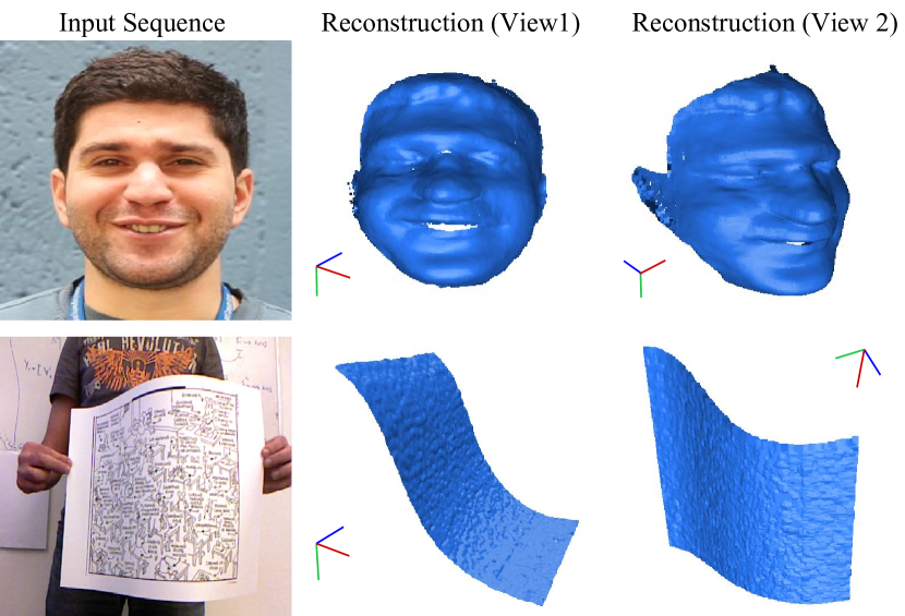
Figure 1: Our algorithm takes dense long-term 2D trajectories of a non-rigid deforming object as input, and provides a dense detailed 3D reconstruction of it. The reconstructed surface captures the complex non-linear motion which can be helpful for real world applications such as 3D virtual and augmented reality. Example frames are taken from publicly available real datasets: real face sequence[18] and kinect_paper sequence[37] respectively.

For many real-world applications, such as facial expression reconstruction, limitations such as scalability, timing, robustness, reliable modeling, etc., are of crucial concern. Despite these limitations, no template-free approach exists that can reliably deal with these concerns. In this paper, we propose a template-free dense NRSfM algorithm that overcomes these difficulties. As a first step to overcome these difficulties, we reduce the overall high-dimensional non-linear space spanned by representing the deforming shape as a union of several local low-dimensional linear subspaces. Our approach is based on a simple idea/assumption i.e., any complex deforming surface can be approximated by a locally linear subspace structure [10]. We use this simple intuition in a spatio-temporal framework to solve dense NRSfM. This choice naturally leads to a few legitimate queries:

a) Why spatio-temporal framework for solving dense NRSfM? Spatio-temporal framework by Kumar et al. [23] has exhibited the state-of-the-art results on the recent NRSfM challenge [5, 21]. A recent method [3] which follows the same idea as proposed by Kumar et al. [23] has also observed an improvement in the reconstruction accuracy under such formulations. Even though the concept behind such a framework is elementary, no algorithm to our knowledge exists that exploit such an intrinsic idea for dense NRSfM.

b) Why the previously proposed spatio-temporal methods are unable to handle dense NRSfM? The formulation proposed by Kumar et al. [23] and its adaptation [3] is inspired from SSC [16], and LRR [30]. As a result, the complexity of their formulations grows exponentially in the order of the number of data points. This makes it difficult to solve dense NRSfM using their formulations. Moreover, these methods [23, 41, 3] use an assumption that non-rigid shape should lie on a low-dimensional linear or affine subspace globally. In reality, such an assumption does not hold for all kinds of non-linear deformations [39, 34]. Although a recent spatio-temporal method proposed by Dai et al. [11] solves this task, it involves a series of least square problems to be solved, which is computationally demanding.

To overcome all these issues, we propose a spatio-temporal dense NRSfM algorithm which is free from such unwarranted assumptions and limitations. Instead, we adhere to the assumption that the low-dimensional linear subspace spanned by a deforming shape is locally valid. Such an assumption about shapes has been well studied in topological manifold theory [1, 15]. The Grassmann manifold is a topologically rich non-linear manifold, each point of which represents the set of all right-invariant subspaces of the Euclidean space. One property of the Grassmannian that is particularly useful in our setting is that the points in it can be embedded into the space of symmetric matrices. This property has been used in several computer vision applications that deal with subspace representation of data [20, 8]. Accordingly, in our problem, to model a non-linear shape, using a Grassmannian allows us to represent the shape as a set of “smooth” low-dimensional surfaces embedded in a higher dimensional Euclidean space. Such a representation not only reduces the complexity of our task but also makes our formulation robust and scalable as described below.

c) Why Grassmann manifold? It is well-known that the complex non-rigid deformations are composed of multiple subspaces that quite often fit a higher-order parametric model [33, 36, 41]. To handle such complex models globally can be very challenging – both numerically and computationally. Consequently, for an appropriate representation of such a model, we decompose the overall non-linearity of the shape by a set of locally linear models that span a low-rank subspace of a vector space. As alluded to above, the space of all $d$-dimensional linear subspaces of $\mathbb{R}^{N}$ ($0<d<N$) forms the Grassmann manifold [1, 2]. Modeling the deformation on this manifold allows us to operate on the number of subspaces rather than on the number of vectorial data points (on the shape), which reduces the complexity of the problem significantly. Moreover, since each local surface is a low-rank subspace, it can be faithfully reconstructed using a few eigenvalues and corresponding eigenvectors, which makes such a representation scalable and robust to noise.

The aforementioned properties of the Grassmannian perfectly fit our strategy to model complex deformations, and therefore, we blend the concept of spatio-temporal representations with local low-rank linear models. This idea results in a two-stage coupled optimization problem i.e., local reconstruction and global grouping, which is solved efficiently using the standard ADMM algorithm [7]. As the local reconstructions are performed using a low-rank eigen decomposition, our representation is computationally efficient and robust to noise. We demonstrate the benefit of our approach to benchmark real and synthetic sequences §5. Our results show that our method outperforms previous state-of-the-art approaches by 1-2 % on all the benchmark datasets. Before we provide the details of our algorithm, we review some pertinent previous works in the next section.

2 Background

This section provides a brief background on the recent advancements in NRSfM, focusing mainly on the methods that are relevant to this work.

Preliminaries: We borrow the notation system from Dai et al.’s work [14] for its wide usage. Given ‘$P$’ feature points over ‘$F$’ frames, we represent $W\in\mathbb{R}^{2F\times P}$, $S\in\mathbb{R}^{3F\times P}$, $R\in\mathbb{R}^{2F\times 3F}$ as the measurement, the shape, and the rotation matrices, respectively. Here $R$ matrix is composed of block diagonal $R_{i}\in\mathbb{R}^{2\times 3}$, representing per frame orthographic camera projection. Also, the notation $S^{\sharp}\in\mathbb{R}^{3P\times F}$ stands for the rearranged shape matrix, which is a linear mapping of $S$. We use $\|\ .\ \|_{F}$ and $\|\ .\ \|_{*}$ to denote the Frobenius norm and the nuclear norm, respectively.

(a) Dai et al.’s [14] $\underset{S^{\sharp},E}{\text{minimize}}~{}\|S^{\sharp}\|_{*}+\lambda\|E\|_{F}^{2}$ subject to: $W=RS+E$	(b) Zhu et al.’s [41] $\underset{S^{\sharp},C,E}{\text{minimize}}~{}\|C\|_{*}+~{}\gamma\|S^{\sharp}\|_{*}+\lambda\|E\|_{1}$ subject to: $S^{\sharp}=S^{\sharp}C,W=RS+E$
(c) Kumar et al.’s [23] $\underset{S,S^{\sharp},C_{1},C_{2}}{\text{minimize}}\frac{1}{2}\|W-RS\|_{F}^{2}+\lambda_{1}\|C_{1}\|_{1}+\lambda_{2}\|S^{\sharp}\|_{*}+\lambda_{3}\|C_{2}\|_{1}$ subject to: $S=SC_{1},S^{\sharp}=S^{\sharp}C_{2},1^{T}C_{1}=1^{T},1^{T}C_{2}=1^{T},$ $diag(C_{1})=0,diag(C_{2})=0,S^{\sharp}=g(S)$	(d) Garg et al.’s[18] $\underset{S,R}{\text{minimize}}\frac{\lambda}{2}\|W-RS\|_{F}^{2}+\sum_{f,i,p}\|\nabla S_{f}^{i}(p)\|+\tau\|S^{\sharp}\|_{*}$ subject to: $R\in\mathbb{SO}(3)$

Table 1: A brief summary of formulation used by some of the recent approaches to solve sparse and dense NRSfM which are closely related to our method. Among all these four methods only Garg et al.’s [18] approach is formulated particularly for solving dense NRSfM.

2.1 Relevant Previous Work

Dai et al.’s approach: Dai et al. proposed a simple and elegant solution to NRSfM [14]. The work, dubbed “prior-free”, provides a practical solution as well as new theoretical insights to NRSfM. Their formulation involves nuclear norm minimization on $S^{\sharp}$ instead of $S$ –see Table 1(a). This is enforced due to the fact that $3K$ rank bound on $S$ is weaker than $K$ rank bound on $S^{\sharp}$, where $K$ refers to the rank of $S$. Although this elegant framework provides robust results for the shapes that span a single subspace, it may perform poorly on complex non-rigid motions [41].

Zhu et al.’s approach: To achieve better 3D reconstructions on complex non-rigid sequences, this work capitalized on the limitations of Dai et al.’s work[14] by exploiting the union of subspaces in the shape space [41]. The proposed formulation is inspired by LRR [30] in conjunction with Dai et al. work –see Table 1(b). In the formulation, $C\in\mathbb{R}^{F\times F}$, $E\in\mathbb{R}^{2F\times P}$ are the coefficient and error matrices.

Kumar et al.’s approach: Kumar et al. exploits multiple subspaces both in the trajectory space and in the shape space [23]. This work demonstrated empirically that procuring multiple subspaces in the trajectory and shape spaces provide better reconstruction results. They proposed a joint segmentation and reconstruction framework, where segmentation inherently benefits reconstruction and vice-versa –see Table 1(c). In their formulation $C_{1}\in\mathbb{R}^{P\times P}$, $C_{2}\in\mathbb{R}^{F\times F}$ are the coefficient matrices and, $g(.)$ linearly maps $S$ to $S^{\sharp}$.

Dense NRSfM approach: Garg et al. developed a variational approach to solve dense NRSfM [18]. The optimization framework proposed by them employs total variational constraint on the deforming shape ($\nabla S_{f}^{i}(p)$) to allow edge preserving discontinuities, and trace norm constraints to penalize the number of independent shapes –see Table 1(d). Recently, Dai et al. has also proposed a dense NRSfM algorithm with a spatio-temporal formulation [11].

2.2 Motivation

This work is intended to overcome the shortcomings of the previous approaches to solve dense NRSfM. Accordingly, we would like to outline the critical limitations associated with them. Although some of them are highlighted before, we reiterate it for the sake of completeness.

1. To solve dense NRSfM using the formulation proposed by Kumar et al. [23] and Zhu et al. [41] is nearly impossible due to the complexity of their formulation §1. Also, the error measure used by them is composed of Euclidean norm defined on the original data (see Table 1), which is not proper for non-linear data with a manifold structure [1, 38].

2. The algorithm proposed by Garg et al. [18] results in a biconvex formulation, which is computationally expensive and needs a GPU to speed up the implementation. Similarly, Dai et al.’s recent work[11] is computationally expensive as well due to costly gradient term in their formulation.

3. Methods such as [40, 29] rely on the template prior for dense 3D reconstruction of the object. Other piecewise approach for solving dense NRSfM [35] require a post-processing step to stitch all the local reconstructions.

To avoid all the aforementioned limitations, we propose a new dense NRSfM algorithm. The primary contributions of this paper are as follows:

1. A scalable spatio-temporal framework on the Grassmann manifold to solve dense NRSfM which does not need any template prior.

2. An effective framework that can handle non-linear deformations even with noisy trajectories and provides state-of-the-art results on benchmark datasets.

3. An efficient solution to the proposed optimization based on the ADMM procedure [7].

3 Problem Formulation

In this section, we first provide a brief introduction to the Grassmann manifold and a suitable definition for a similarity distance metric on it, before revealing our formulation.

3.1 Grassmann Manifold

The Grassmann manifold, usually denoted as $\mathcal{G}(n,r)$, consists of all $r$-dimensional linear subspaces of $\mathbb{R}^{n}$, where $n>r$. A point on the Grassmann manifold is represented by a $n\times r$ matrix (say $X$), whose columns are composed of orthonormal basis of the subspace spanned by $X$, denoted as $\mathbf{span}(X)$ or in short as [$X$]. Let’s suppose [$X_{1}$], [$X_{2}$] are two such points on this manifold, then among several similarity distances known for this manifold [20], we will be using the projection metric distance given by $\small{d_{g}([X_{1}],[X_{2}])=\frac{1}{\sqrt[]{2}}\|X_{1}X_{1}^{T}-X_{2}X_{2}^{T}\|_{F}}$, as it allows directly embedding the Grassmannian points into a Euclidean space (and the use of the Frobenius norm) using the mapping $X\rightarrow XX^{T}$. With this metric, $(\mathcal{G},d_{g})$ forms a metric space. Interested readers may refer to [20] for details.

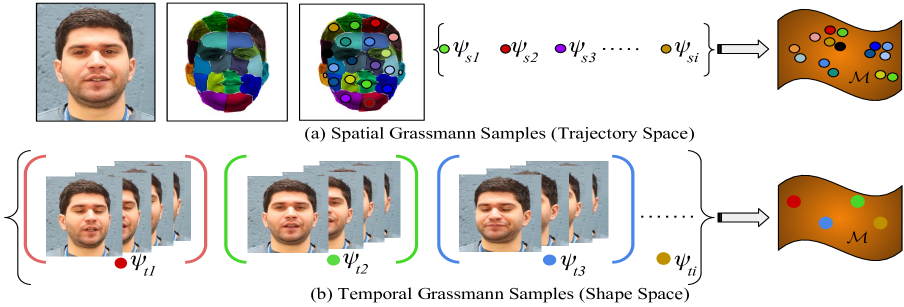
Figure 2: Conceptual illustration of data point representation on the grassmann manifold. Each local subspace can equivalently be represented by a single point on the manifold. Top row: Construction of grassmann samples in the trajectory space using spatial information. Bottom row: Construction of grassmann samples in the shape space by partitioning the shapes in a sequential order over frames.

3.2 Formulation

With the relevant background as reviewed in the above sections, we are now ready to present our algorithm to solve the dense NRSfM task under orthographic projection. We start our discussion with the classical representation to NRSfM i.e.,

$$\small W_{s}=RS_{s}$$ (1)

where, $W_{s}\in\mathbb{R}^{2F\times P}$, $R={\text{blkdiag}}(R_{1},...,R_{F})\in\mathbb{R}^{2F\times 3F}$, $S_{s}\in\mathbb{R}^{3F\times P}$. The motive here is, given the input measurement matrix, solve for rotation ($R$) and 3D shape ($S_{s}$). To serve this objective, Eq.(1) maintains the camera motion and the shape deformation such that it complies with the image measurements. For our method, we solve for rotations using the Intersection method [14] by assuming that the multiple non-rigid motions within a single deforming object, over frames, can be faithfully approximated by per frame single relative camera motion with a higher rank. Accordingly, our goal reduces to develop a systematic approach that can reliably explain the non-rigid shape deformations and provides better 3D reconstruction. We use subscript ‘$s$’ in Eq.(1) to indicate that the column permutations of $S_{s}$ and $W_{s}$ matrix are allowed. However, the column permutations of $S_{t}^{\sharp}$ is inadmissible as it results in discontinuous trajectories over frames.

Grassmannian Representations in Trajectory Space: Let’s suppose $\mathbf{\Psi}_{s}$ = $\{{\it{\Psi_{s1}}},{\it{\Psi_{s2}}},..{\it{\Psi_{sK_{s}}}}\}$ is the set of points on the Grassmann manifold generated using $S_{s}$ matrix, then ${\bf{\mathcal{T}}}_{s}=\big{\{}(\mathit{\Psi_{s1}})(\mathit{\Psi_{s1}})^{T},(\mathit{\Psi_{s2}})(\mathit{\Psi_{s2}})^{T}...,(\mathit{\Psi_{sK_{s}}})(\mathit{\Psi_{sK_{s}}})^{T}\big{\}}$ represents a tensor which is constructed by mapping all symmetric matrices of the Grassmann data points —refer Figure 2(a). As discussed before in §1, to explain the complex deformations, we reduce the overall non-linear space as a union of several local low-dimensional linear spaces which form the sample points on the Grassmann manifold. But, the notion of self-expressiveness is valid only for Euclidean linear or affine subspace. To apply self-expressiveness on the Grassmann manifold one has to adopt linearity onto the manifold. Since, Grassmann manifold is isometrically equivalent to the symmetric idempotent matrices [9], we embed the Grassmann manifold into the symmetric matrix manifold, where the self-expression can be defined in the embedding space. This leads to the following optimization:

$$\underset{E_{s},C_{s}}{\text{minimize}}~{}\|E_{s}\|_{F}^{2}+\lambda_{1}\|C_{s}\|_{*}$$ (2)

$$\text{\it{subject to:}}~{}{\bf{\mathcal{T}}}_{s}={\bf{\mathcal{T}}}_{s}C_{s}+E_{s}$$

We denote $C_{s}\in\mathbb{R}^{K_{s}\times K_{s}}$ as the coefficient matrix with ‘$K_{s}$’ as the total number of spatial groups. Here, $E_{s}$ measures the trajectory group reconstruction error as per the manifold geometry. Also, we would like to emphasize that since the object undergoes deformations in the 3D space, we operate in 3D space rather than in the projected 2D space. $\|~{}\|_{*}$ is enforced on $C_{s}$ for a low-rank solution.

Grassmannian Representations in Shape Space: Deforming object attains different state over time which adheres to distinct temporal local subspaces [23]. Assuming that the temporal deformation is smooth over-time, we express deforming shapes in terms of local self-expressiveness across frames as:

$$\underset{E_{t},C_{t}}{\text{minimize}}~{}\|E_{t}\|_{F}^{2}+\lambda_{2}\|C_{t}\|_{*}$$ (3)

$$\text{\it{subject to:}}{\bf{\mathcal{T}}}_{t}={\bf{\mathcal{T}}}_{t}C_{t}+E_{t}$$

Similarly, ${\bf{\mathcal{T}}}_{t}$ is the set of all symmetric matrices constructed using a set of Grassmannian samples $\mathbf{\Psi}_{t}$, where $\mathbf{\Psi}_{t}$ contains the samples which are drawn from $S_{t}^{\sharp}\in\mathbb{R}^{3P\times F}$ —refer Figure 2(b). Intuitively, $S_{t}^{\sharp}$ is a shape matrix with each column as a deforming shape. $E_{t}$, $C_{t}\in\mathbb{R}^{K_{t}\times K_{t}}$ represent the temporal group reconstruction error and coefficient matrix respectively, with $K_{t}$ as the number of temporal groups. $\|~{}\|_{*}$ is enforced on $C_{t}$ for a low-rank solution.

Spatio-Temporal Formulation: Combining the above two objectives and their constraints with reprojection error term give us our formulation. Our representation blends the local subspaces structure along with the global composition of a non-rigid shape. Thus, the overall objective is:

$$\underset{S_{s},S_{t}^{\sharp},E_{s},E_{t},C_{s},C_{t}}{\text{minimize}}\mathbf{E}=\frac{1}{2}~{}\|W_{s}-RS_{s}\|_{F}^{2}+\gamma\|S_{t}^{\sharp}\|_{*}+\lambda_{1}\|E_{s}\|_{F}^{2}$$ (4)

$$+\lambda_{2}\|E_{t}\|_{F}^{2}+\lambda_{3}\|C_{s}\|_{*}+\lambda_{4}\|C_{t}\|_{*}$$

$$\text{\it{subject to:}}~{}{\bf{\mathcal{T}}}_{s}={\bf{\mathcal{T}}}_{s}C_{s}+E_{s};{\bf{\mathcal{T}}}_{t}={\bf{\mathcal{T}}}_{t}C_{t}+E_{t};$$

$$\hskip 38.74985pt\mathbf{\Psi}_{s}=\mathit{\xi(C_{s},S_{s},\sigma_{\epsilon})};\mathbf{\Psi}_{t}=\mathit{\xi(C_{t},S_{t}^{\sharp},\sigma_{\epsilon})};$$

$$\hskip 38.74985ptS_{s}=\zeta\big{(}\mathbf{\Psi}_{s},\Sigma_{s},V_{s},N_{s});S_{t}^{\sharp}=\zeta\big{(}\mathbf{\Psi}_{t},\Sigma_{t}^{\sharp},V_{t},N_{t});$$

$$\hskip 38.74985ptS_{t}^{\sharp}=\mathscr{T}_{1}(S_{s});W_{s}=\mathscr{T}_{2}(W_{s},S_{s});$$

The re-projection error constraint performs the 3D reconstruction using $W_{s}$ and $R$. Meanwhile, the local subspace grouping naturally enforces the union of subspace structure in $S_{s}$, $S_{t}^{\sharp}$ with corresponding low-rank representations of the coefficient matrices $C_{s}$ and $C_{t}$. Here, the function $\xi(.)$ draws inference from $C$ matrices to refine Grassmannian sample set, both in trajectory and shape spaces. The function $\zeta(.)$ reconstructs $S_{s}$ and $S_{t}^{\sharp}$ matrices based on a set of local subspaces ($\mathbf{\Psi}_{s},\mathbf{\Psi}_{t},V_{s},V_{t}$), singular values ($\Sigma_{s}$, $\Sigma_{t}$) and the number of top eigenvalues ($N_{s},N_{t}$). The function $\mathscr{T}_{1}(.)$ transforms $S_{s}\in\mathbb{R}^{3F\times P}$ matrix to $S_{t}^{\sharp}\in\mathbb{R}^{3P\times F}$ matrix and $\mathscr{T}_{2}(.)$ function rearranges $W_{s}$ matrix as per the recent ordering of $S_{s}$. Parameters such as ‘$\sigma_{\epsilon}$’, ‘$N_{s}$’ and ‘$N_{t}$’ provides the flexibility to handle noise and adjust computations. Note that the element of the sets $\mathbf{\Psi}_{s},\mathbf{\Psi}_{t},V_{s}~{}\text{and}~{}V_{t}$ are obtained using SVD. The above equation i.e. Eq: (4) is a coupled optimization problem where the solution to $S$ matrices influence the solution of $C$ matrices and vice-versa, and ${\small\mathscr{T}_{1}}()$ connects $S_{t}^{\sharp}$ to $S_{s}$.

Algorithm 1 Scalable Dense Non-Rigid Structure from Motion: A Grassmannian Perspective

0:  $W_{s}$, $R$ using [14], tuning parameters: $\lambda_{1}$, $\lambda_{2}$, $\lambda_{3}$, $\lambda_{4}$, $\gamma$, $\rho=1.1$, $\beta=1e^{-3}$, $\beta_{m}=1e^{6}$, $\epsilon=1e^{-12}$, $K_{s}$, $K_{t}$.Initialize: $S_{s}$ = pseudoinverse($R$)$W_{s}$ and ${S^{\sharp}_{t}}=\mathscr{T}_{1}(S_{s})$.Initialize: ‘$K_{t}$’ temporal data points on the Grassmann manifold using ‘${S^{\sharp}_{t}}$’ matrix, $\mathbf{\Psi}_{t}$ = $\{\it{\Psi_{ti}}\}_{i=1}^{K_{t}}$.Initialize: ‘$K_{s}$’ spatial data points on the Grassmann manifold using ‘${S_{s}}$’ matrix, $\mathbf{\Psi}_{s}$ = $\{\it{\Psi_{si}}\}_{i=1}^{K_{s}}$.Initialize: The auxiliary variables $J_{s}$, $J_{t}$ and Lagrange multiplier $\{Y_{i}\}_{i=1}^{3}$ as zero matrices.Initialize: $\Omega_{ij}^{s}$ = $trace[\big{(}{\it{\Psi_{sj}^{T}}}{\it{\Psi_{si}}}\big{)}\big{(}{\it{\Psi_{si}^{T}}}{\it{\Psi_{sj}}}\big{)}]$, $\Omega_{ij}^{t}$ = $trace[\big{(}{\it{\Psi_{tj}^{T}}}{\it{\Psi_{ti}}}\big{)}\big{(}{\it{\Psi_{ti}^{T}}}{\it{\Psi_{tj}}}\big{)}]$, $\mathbf{\Omega}_{s}=(\Omega_{ij}^{s})_{i,j=1}^{K_{s}}$, $\mathbf{\Omega}_{t}=(\Omega_{ij}^{t})_{i,j=1}^{K_{t}}$            $L_{s}L_{s}^{T}$ = Cholesky($\mathbf{\Omega}_{s}$), $L_{t}L_{t}^{T}$ = Cholesky($\mathbf{\Omega}_{t}$)

1:  while not converged do

2:     $S_{s}$ $\leftarrow$ $\Big{(}\beta\big{(}\mathscr{T}_{1}^{-1}(S_{t}^{\sharp})+\frac{\mathscr{T}_{1}^{-1}(Y_{1})}{\beta}\big{)}+R^{T}W_{s}\Big{)}\big{/}(R^{T}R+\beta I)$

3:     $C_{s}$ $\leftarrow$ $\Big{(}2\lambda_{1}L_{s}L_{s}^{T}+\beta(J_{s}-\frac{Y_{2}}{\beta})\Big{)}$ $\big{(}2\lambda_{1}L_{s}L_{s}^{T}+\beta I_{s}\big{)}^{-1}$

4:     $\mathbf{\Psi}_{s}$ $\leftarrow$ $\xi(C_{s},S_{s},\sigma_{\epsilon})$                            // Update spatial Grassmann points

5:     $S_{s}$ $\leftarrow$ $\zeta(\mathbf{\Psi}_{s},\Sigma_{s},V_{s},N_{s})$;                   // refine based on top $N_{s}$ eigen value

6:     $J_{s}$ $\leftarrow$ $U_{J_{s}}\mathcal{S}_{\frac{\lambda_{3}}{\beta}}(\Sigma_{J_{s}})V_{J_{s}}$, where $[U_{J_{s}},\Sigma_{J_{s}},V_{J_{s}}]=\emph{svd}(C_{s}+\frac{Y_{2}}{\beta})$ and $\mathcal{S}_{\tau}[x]$ = sign(x)max($|x|$-$\tau$, 0)

7:     $S_{t}^{\sharp}$ $\leftarrow$ $U_{t}\mathcal{S}_{\frac{\gamma}{\beta}}(\Sigma_{t})V_{t}$, where $[U_{t},\Sigma_{t},V_{t}]=\emph{svd}(\mathscr{T}_{1}(S_{s})-\frac{Y_{1}}{\beta})$ and $\mathcal{S}_{\tau}[x]$ = sign(x)max($|x|$-$\tau$, 0)

8:     $C_{t}$ $\leftarrow$ $\Big{(}2\lambda_{2}L_{t}L_{t}^{T}+\beta(J_{t}-\frac{Y_{3}}{\beta})\Big{)}$ $\big{(}2\lambda_{2}L_{t}L_{t}^{T}+\beta I_{t}\big{)}^{-1}$

9:     $\mathbf{\Psi}_{t}$ $\leftarrow$ $\xi(C_{t},S_{t}^{\sharp},\sigma_{\epsilon})$ // Update temporal Grassmann points

10:     $S_{t}^{\sharp}$ $\leftarrow$ $\zeta(\mathbf{\Psi}_{t},\Sigma_{t},V_{t},N_{t})$;                  // refine based on top $N_{t}$ eigen value

11:     $J_{t}$ $\leftarrow$ $U_{J_{t}}\mathcal{S}_{\frac{\lambda_{4}}{\beta}}(\Sigma_{J_{t}})V_{J_{t}}$, where $[U_{J_{t}},\Sigma_{J_{t}},V_{J_{t}}]=\emph{svd}(C_{t}+\frac{Y_{3}}{\beta})$ and $\mathcal{S}_{\tau}[x]$ = sign(x)max($|x|$-$\tau$, 0)

12:     $\Omega_{ij}^{s}$ $\leftarrow$ $trace[\big{(}{\it{\Psi_{sj}^{T}}}{\it{\Psi_{si}}}\big{)}\big{(}{\it{\Psi_{si}^{T}}}{\it{\Psi_{sj}}}\big{)}]$, $\Omega_{ij}^{t}$ $\leftarrow$ $trace[\big{(}{\it{\Psi_{tj}^{T}}}{\it{\Psi_{ti}}}\big{)}\big{(}{\it{\Psi_{ti}^{T}}}{\it{\Psi_{tj}}}\big{)}]$;

13:     $\mathbf{\Omega}_{s}\leftarrow(\Omega_{ij}^{s})_{i,j=1}^{K_{s}}$, $\mathbf{\Omega}_{t}\leftarrow(\Omega_{ij}^{t})_{i,j=1}^{K_{t}}$;// . $\mathbf{\Omega}_{s}\succeq 0,\mathbf{\Omega}_{t}\succeq 0$, if $\mathbf{\Omega}_{s}||\mathbf{\Omega}_{t}=0$ add $\delta\mathbf{I}$ to make it $\succ 0$ (see suppl. material)

14:     $L_{s}L_{s}^{T}$ = Cholesky($\mathbf{\Omega}_{s}$), $L_{t}L_{t}^{T}$ = Cholesky($\mathbf{\Omega}_{t}$);

15:     $W_{s}$ $\leftarrow$ $\mathscr{T}_{2}(W_{s},S_{s})$                  // Note: Column permutation for $W_{s}$ and $S_{s}$ should be same.

16:     $Y_{1}$ := $Y_{1}+\beta(S_{t}^{\sharp}-\mathscr{T}_{1}(S_{s}))$, $Y_{2}$ := $Y_{2}+\beta(C_{s}-J_{s})$, $Y_{3}$ := $Y_{3}+\beta(C_{t}-J_{t})$; // Update Lagrange multipliers

17:     $\beta\leftarrow\text{minimum}(\rho\beta,\beta_{m})$

18:     maxgap := maximum($[\|S_{t}^{\sharp}-\mathscr{T}_{1}(S_{s})\|_{\infty},\|C_{s}-J_{s}\|_{\infty},\|C_{t}-J_{t}\|_{\infty}]$)

19:     if (maxgap $<$ $\epsilon$ $\parallel\beta>\beta_{m}$) then

20:        break;

21:     end if// check for the convergence

22:  end while// Note: $\delta$ is a very small positive number and $\mathbf{I}$ symbolizes identity matrix.

22:  $S_{s}$, $S_{t}$, $C_{s}$, $C_{t}$. // Note: Kindly use economical version of svd on a regular desktop.

4 Solution

The formulation in Eq.(4) is a non-convex problem due to the bilinear optimization variables (${\bf{\mathcal{T}}}_{s}C_{s}$, ${\bf{\mathcal{T}}}_{t}C_{t}$), hence a global optimal solution is hard to achieve. However, it can be efficiently solved using Augmented Lagrangian Methods (ALMs) [7], which has proven its effectiveness for many non-convex problems. Introducing Lagrange multipliers $(\{Y_{i}\}_{i=1}^{3})$ and auxiliary variables $(J_{s},J_{t})$ to Eq.(4) gives us the complete cost function as follows:

$$\underset{S_{s},S_{t}^{\sharp},C_{s},C_{t},J_{s},J_{t}}{\text{minimize}}\mathbf{E}=\frac{1}{2}~{}\|W_{s}-RS_{s}\|_{F}^{2}+\frac{\beta}{2}\|S_{t}^{\sharp}-\mathscr{T}_{1}(S_{s})\|_{F}^{2}+$$ (5)

$$<Y_{1},S_{t}^{\sharp}-\mathscr{T}_{1}(S_{s})>+\gamma\|S_{t}^{\sharp}\|_{*}+\lambda_{1}\|{\bf{\mathcal{T}}}_{s}-{\bf{\mathcal{T}}}_{s}C_{s}\|_{F}^{2}+\lambda_{3}\|J_{s}\|_{*}$$

$$+\frac{\beta}{2}\|C_{s}-J_{s}\|_{F}^{2}+<Y_{2},C_{s}-J_{s}>+\lambda_{2}\|{\bf{\mathcal{T}}}_{t}-{\bf{\mathcal{T}}}_{t}C_{t}\|_{F}^{2}+$$

$$\lambda_{4}\|J_{t}\|_{*}+\frac{\beta}{2}\|C_{t}-J_{t}\|_{F}^{2}+<Y_{3},C_{t}-J_{t}>$$

$$\text{\it{subject to:}}~{}\mathbf{\Psi}_{s}=\mathit{\xi(C_{s},S_{s},\sigma_{\epsilon})};\mathbf{\Psi}_{t}=\mathit{\xi(C_{t},S_{t}^{\sharp},\sigma_{\epsilon})};$$

$$\hskip 38.74985ptS_{s}=\zeta(\mathbf{\Psi}_{s},\Sigma_{s},V_{s},N_{s});S_{t}^{\sharp}=\zeta(\mathbf{\Psi}_{t},\Sigma_{t}^{\sharp},V_{t},N_{t});$$

$$\hskip 38.74985ptW_{s}=\mathscr{T}_{2}(W_{s},S_{s});$$

The function $\xi(.)$ first computes the SVD of $C$ matrices, i.e. $C=[U_{c},\Sigma_{c},V_{c}]$, then forms a matrix $A$ such that $A_{ij}=[XX^{T}]_{ij}^{\sigma_{\epsilon}}$, where $\sigma_{\epsilon}$ is set empirically based on noise levels and $X=U_{c}(\Sigma_{c})^{0.5}$ (normalized). Secondly, it uses $A_{ij}$ to form new Grassmann samples from the $S$ matrices[22]. Notice that $\xi(.)$ operates on $C$ matrices whose dimensions depend on the number of Grassmann samples. This reduces the complexity of the task from exponential in the number of vectorial points to exponential in the number of linear subspaces. The later being of the order 10-50, where as the former can go more than 50,000 for dense NRSfM.

The $\zeta(.)$ function is defined as follows $\zeta$ = $\big{\{}(\mathbf{\Psi}_{a},\Sigma_{a},V_{a},r)|S_{a}$ = $\mathbf{horzcat}(\mathbf{\Psi}_{a}^{r}\Sigma_{a}^{r}V_{a}^{r}),\forall 1\leq a\leq\mathbf{Card}(\mathbf{\Psi}_{a}),r\in\mathbb{Z}^{+}\big{\}}$, where $r$ stands for top-$r$ eigenvalues, $\mathbf{Card}(.)$ denotes the cardinal number of the set and $\mathbf{horzcat}(.)$ denotes for the horizontal concatenation of matrices. Intuitively, $\zeta(.)$ reconstructs back each local low-rank subspace. During implementation, we use $S_{s}$, $S_{t}^{\sharp}$ in place of $S_{a}$ accordingly. The optimization variables over iteration are obtained by solving for one variable at a time treating others as constant, keeping the constraints intact. For detailed derivations for each sub-problem and proofs, kindly refer to the supplementary material. The pseudo code of our implementation is provided in Algorithm 1.

5 Experiments and Results

We compare the performance of our method against four previously reported state-of-the-art approaches, namely Dense Spatio-Temporal DS [11], Dense Variational DV [18], Trajectory Basis PTA [4] and Metric Projection MP [32]. To test the performance, we used dense NRSfM dataset introduced by Garg et al. [18] and Varol et al. [37] under noisy and noise free conditions. For quantitative evaluation of 3D reconstruction, we align the estimated shape $S_{est}^{t}$ with ground-truth shape $S_{GT}^{t}$ per frame using Procrustes analysis. We compute the average RMS 3D reconstruction error as $e_{3D}=\frac{1}{F}\sum_{t=1}^{F}\frac{\|S_{est}^{t}-S_{GT}^{t}\|_{F}}{\|S_{GT}^{t}\|_{F}}$. We used Kmeans++ algorithm [6] to initialize segments without disturbing the temporal continuity.

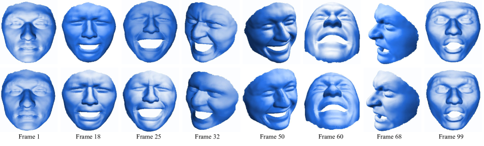
Figure 3: Reconstruction results obtained on synthetic dense face dataset (face sequence 4). Top row : Ground-truth 3D points, Bottom row : Recovered 3D points using our approach.

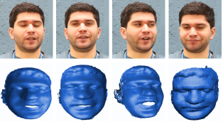
(a)

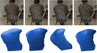
(b)

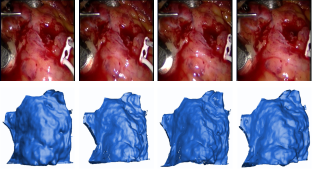
(c)

Figure 4: Qualitative reconstruction results procured on benchmark real dense dataset [18] a) Face sequence (28,332 feature points over 120 frames) b) Back sequence (20,561 feature points over 150 frames) c) Heart sequence (68,295 feature points over 80 frames).

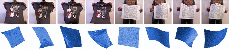
Figure 5: Reconstruction results on benchmark kinect_tshirt (74,000 points, 313 frames) and kinect_paper(58,000 points, 193 frames) dataset [37]. Top row: Input image frame. Bottom row: Dense 3D reconstruction for the corresponding frame using our approach.

Experiments on Synthetic Face Sequences: This dataset consists of 4 different face sequence with 28,880 feature points tracked over multiple frames. The face sequence 1, 2 is a 10 frame long video, whereas, face sequence 3, 4 is a 99 frame long video. It’s a challenging dataset mainly due to different rotation frequencies and deformations in each of the sequence. Figure 3 shows the qualitative reconstruction results obtained using our approach in comparison to the ground-truth for face sequence 4. Table 2 lists the performance comparisons of our method with other competing methods. Clearly, our algorithm outperforms the other baseline approach, which helps us to conclude that holistic approaches to rank minimization without drawing any inference from local subspace structure is a less effective framework to cope up with the local non-linearities.

Data	DS [11]	DV [18]	PTA [4]	MP [32]	Ours
Seq.1	0.0636	0.0531	0.1559	0.2572	0.0443
Seq.2	0.0569	0.0457	0.1503	0.0640	0.0381
Seq.3	0.0374	0.0346	0.1252	0.0611	0.0294
Seq.4	0.0428	0.0379	0.1348	0.0762	0.0309

Table 2: Average 3D reconstruction error ($e_{3D}$) comparison on dense synthetic face sequence[18]. Note: The code for DV [18] is not publicly available, we tabulated its results from DS [11] work.

Experiments on face, back and heart sequence: This dataset contains monocular videos of human facial expressions, back deformations, and beating heart under natural lighting conditions. The face sequence, back sequence, and heart sequence are composed of 28332, 20561, and 68295 feature points tracked over 120, 150, and 80 images, respectively. Unfortunately, due to the lack of ground-truth 3D data, we are unable to quantify the performance of these sequences. Figure 4 shows some qualitative results obtained using our algorithm on this real dataset.

Experiments on kinect_paper and kinect_tshirt sequence: To evaluate our performance on the real deforming surfaces, we used kinect_paper and kinect_tshirt dataset[37]. This dataset provides sparse SIFT[31] feature tracks along with dense 3D point clouds of the entire scene for each frame. Since, dense 2D tracks are not directly available with this dataset, we synthesized it. To obtain dense feature tracks, we considered the region within a window containing the deforming surface. Precisely, we considered the region within $xw$ = (253, 253, 508, 508), $yw$ = (132, 363, 363, 132) across 193 frames for paper sequence, and $xw$ = (203, 203, 468, 468), $yw$ = (112, 403, 403, 112) across 313 frames for tshirt sequence to obtain the measurement matrix [19, 17]. Figure 5 show some qualitative results obtained using our method on this dataset. Table 3 lists the numerical comparison of our approach with other competing dense NRSfM approaches on this dataset.

Data	DS [11]	DV [18]	PTA [4]	MP [32]	Ours
paper	0.0612	-	0.0918	0.0827	0.0394
tshirt	0.0636	-	0.0712	0.0741	0.0362

Table 3: Average 3D reconstruction error ($e_{3D}$) comparison on kinect_paper and kinect_tshirt [37] sequence. Note: The code for DV [18] is not publicly available. The pixels with no 3D data available were discarded for the experiments and the evaluation.

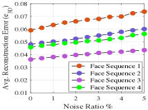
(a)

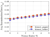
(b)

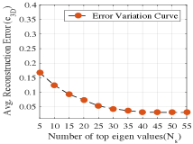
(c)

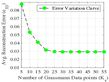
(d)

Figure 6: (a)-(b) Avg. 3D reconstruction error ($e_{3D}$) variation with the change in the noise ratio for synthetic face sequence and kinect sequence respectively. (c)-(d) Variation in $e_{3D}$ with the number of top eigen value and number of grassmann data points for Face Seq3.

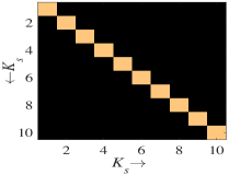
(a)

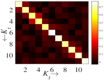
(b)

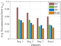
(c)

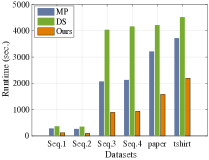
(d)

Figure 7: (a)-(b) A typical structure of $C_{s}\in\mathbb{R}^{K_{s}\times K_{s}}$, $C_{t}\in\mathbb{R}^{K_{t}\times K_{t}}$ after convergence. (c) Ablation test performance on the synthetic face sequence [18]. (d) Runtime comparison of our method with MP [32] and a recent state-of-the-art dense NRSfM algorithm DS[11].

Experiments on noisy data: To evaluate the robustness of our method to noise levels, we performed experiments by adding Gaussian noise under different standard deviations to the measurement matrix. Similar to DS [11] the standard deviations are incorporated as $\sigma_{n}=r\ \text{max}\{|W_{s}|\}$ by varying $r$ from 0.01 to 0.05. We repeated the experiment 10 times. Figure 6(a) and Figure 6(b) shows the variation in the performance of our method under different noise ratio’s on synthetic face sequences[18] and kinect sequences[37] respectively. It can be inferred from the plot that even with large noise ratios, the average reconstruction error does not fluctuate significantly. This improvement is expected from our framework as it is susceptible only to top eigen values.

Effects of variable initialization on the overall performance: We performed several other experiments to study the behavior of our algorithm under different variable initializations. For easy exposition, we conducted this experiment on noise free sequences. We mainly investigated the behavior of $N_{s},N_{t},K_{s},K_{t}$ on the overall performance of our algorithm. Figure 6(c) and Figure 6(d) shows the variations in the reconstruction errors with respect to $N_{s}$ and $K_{s}$ respectively. A similar trend in the plots is observed for changes on $N_{t}$ and $K_{t}$ values. These plots clearly illustrate the usefulness of our local low-rank structure i.e., considering a small number of eigenvalues for every local structure is as good as considering all eigenvalues. Similarly, increasing the number of local subspaces after a certain value has negligible effect on the overall reconstruction error. Furthermore, we examined the form of $C_{s}$ and $C_{t}$ after convergence as shown Figure 7(a) and Figure 7(b). Unfortunately, due to the lack of ground-truth data on local subspaces, we could not quantify $C_{s}$ and $C_{t}$. For qualitative analysis on the observation, kindly refer to the supplementary material.

Ablation Analysis: This test is performed to evaluate the importance of spatial and temporal constraints in our formulation. To do this, we observe the performance of our formulation under four different setups: a) without any spatio-temporal constraint (NC), b) with only spatial constraint (SP), c) with only temporal constraint (TP), and d) with spatio-temporal constraint (Both). Figure 7(c) shows the variations in reconstruction errors under these setups on four synthetic face sequence. The statistics clearly illustrate the importance of both constraints in our formulation.

Runtime Analysis: This experiment is performed on a computer with an Intel core i7 processor and 16GB RAM. The script to compute the runtime is written in MATLAB 2016b. Figure 7(d) shows the runtime comparisons of our approach with other dense NRSfM methods. The runtime reported in Figure 7(d) corresponds to the results listed in Table 2, 3. The results clearly show the scalability of our method on datasets with more than 50,000 points. Despite PTA [4] is faster than our approach, its accuracy suffers by a large margin for dense NRSfM (see Table 2, 3).

6 Conclusion

In this paper, we have introduced a scalable dense NRSfM algorithm which efficiently models the complex non-linear deformations. We achieved this by exploiting the non-linearity on the Grassmann manifold via a spatio-temporal formulation. Moreover, we provided an efficient ADMM [7] based solution for solving our optimization. In the future, we will consider how to extend this work to the projective setting with perspective cameras (e.g. [13, 12]).

Acknowledgement.   S. Kumar was supported in part by Australian Research Council (ARC) grant (DE140100180). Y. Dai was supported in part by National 1000 Young Talents Plan of China, Natural Science Foundation of China (61420106007), and ARC grant (DE140100180). H. Li is funded in part by ARC Centre of Excellence for Robotic Vision (CE140100016).

References

- [1] P.-A. Absil, R. Mahony, and R. Sepulchre. Riemannian geometry of grassmann manifolds with a view on algorithmic computation. Acta Applicandae Mathematicae, 80(2):199–220, 2004.
- [2] P.-A. Absil, R. Mahony, and R. Sepulchre. Optimization algorithms on matrix manifolds. Princeton University Press, 2009.
- [3] A. Agudo and F. Moreno-Noguer. Dust: Dual union of spatio-temporal subspaces for monocular multiple object 3d reconstruction. In IEEE Conference on Computer Vision and Pattern Recognition, 2017.
- [4] I. Akhter, Y. Sheikh, S. Khan, and T. Kanade. Nonrigid structure from motion in trajectory space. In Advances in neural information processing systems, pages 41–48, 2009.
- [5] B. Alessio, Del, A. Henrik, J. Sebastian N, and S. Yaser. Non-rigid structure from motion challenge. IEEE Conference on Computer Vision and Pattern Recognition, 2017.
- [6] D. Arthur and S. Vassilvitskii. k-means++: The advantages of careful seeding. In Proceedings of the eighteenth annual ACM-SIAM symposium on Discrete algorithms, pages 1027–1035. Society for Industrial and Applied Mathematics, 2007.
- [7] S. Boyd, N. Parikh, E. Chu, B. Peleato, and J. Eckstein. Distributed optimization and statistical learning via the alternating direction method of multipliers. Foundations and Trends® in Machine Learning, 3(1):1–122, 2011.
- [8] H. E. Cetingul and R. Vidal. Intrinsic mean shift for clustering on stiefel and grassmann manifolds. In IEEE Conference on Computer Vision and Pattern Recognition, pages 1896–1902, 2009.
- [9] Y. Chikuse. Statistics on special manifolds, volume 174. Springer Science & Business Media, 2012.
- [10] K. Crane. Conformal geometry processing. California Institute of Technology, 2013.
- [11] Y. Dai, H. Deng, and M. He. Dense non-rigid structure-from-motion made easy-a spatial-temporal smoothness based solution. arXiv preprint arXiv:1706.08629, 2017.
- [12] Y. Dai, H. Li, and M. He. Element-wise factorization for n-view projective reconstruction. In ECCV, 2010.
- [13] Y. Dai, H. Li, and M. He. Projective multiview structure and motion from element-wise factorization. IEEE Transactions on Pattern Analysis and Machine Intelligence, 35(9):2238–2251, 2013.
- [14] Y. Dai, H. Li, and M. He. A simple prior-free method for non-rigid structure-from-motion factorization. International Journal of Computer Vision, 107(2):101–122, 2014.
- [15] P. Dollár, V. Rabaud, and S. Belongie. Non-isometric manifold learning: Analysis and an algorithm. In International Conference on Machine Learning, pages 241–248, 2007.
- [16] E. Elhamifar and R. Vidal. Sparse subspace clustering. In IEEE Conference on Computer Vision and Pattern Recognition,, pages 2790–2797. IEEE, 2009.
- [17] R. Garg, A. Roussos, and L. Agapito. Robust trajectory-space tv-l1 optical flow for non-rigid sequences. In Energy Minimization Methods in Computer Vision and Pattern Recognition, pages 300–314. Springer, 2011.
- [18] R. Garg, A. Roussos, and L. Agapito. Dense variational reconstruction of non-rigid surfaces from monocular video. In IEEE Conference on Computer Vision and Pattern Recognition, pages 1272–1279, 2013.
- [19] R. Garg, A. Roussos, and L. Agapito. A variational approach to video registration with subspace constraints. International journal of computer vision, 104(3):286–314, 2013.
- [20] J. Hamm and D. D. Lee. Grassmann discriminant analysis: a unifying view on subspace-based learning. In International conference on Machine learning, pages 376–383. ACM, 2008.
- [21] S. H. N. Jensen, A. Del Bue, M. E. B. Doest, and H. Aanæs. A benchmark and evaluation of non-rigid structure from motion. arXiv preprint arXiv:1801.08388, 2018.
- [22] P. Ji, M. Salzmann, and H. Li. Efficient dense subspace clustering. In IEEE Winter Conference on Applications of Computer Vision, pages 461–468, 2014.
- [23] S. Kumar, Y. Dai, and H.Li. Spatio-temporal union of subspaces for multi-body non-rigid structure-from-motion. Pattern Recognition, 71:428–443, May 2017.
- [24] S. Kumar, Y. Dai, and H. Li. Multi-body non-rigid structure-from-motion. In 3D Vision (3DV), 2016 Fourth International Conference on, pages 148–156. IEEE, 2016.
- [25] S. Kumar, Y. Dai, and H. Li. Monocular dense 3d reconstruction of a complex dynamic scene from two perspective frames. In IEEE International Conference on Computer Vision, pages 4649–4657, Oct 2017.
- [26] W. Kusakunniran, Q. Wu, H. Li, and J. Zhang. Automatic gait recognition using weighted binary pattern on video. In IEEE AVSS, 2009.
- [27] W. Kusakunniran, Q. Wu, J. Zhang, H. Li, and L. Wang. Recognizing gaits across views through correlated motion co-clustering. TIP, 23(2):696–709, 2014.
- [28] M. Lee, J. Cho, C.-H. Choi, and S. Oh. Procrustean normal distribution for non-rigid structure from motion. In IEEE Conference on Computer Vision and Pattern Recognition, pages 1280–1287, 2013.
- [29] H. Li, B. Adams, L. J. Guibas, and M. Pauly. Robust single-view geometry and motion reconstruction. In ACM Transactions on Graphics, volume 28, page 175, 2009.
- [30] G. Liu, Z. Lin, S. Yan, J. Sun, Y. Yu, and Y. Ma. Robust recovery of subspace structures by low-rank representation. IEEE Transactions on Pattern Analysis and Machine Intelligence, 35(1):171–184, 2013.
- [31] D. G. Lowe. Object recognition from local scale-invariant features. In IEEE International Conference on Computer vision, pages 1150–1157, 1999.
- [32] M. Paladini, A. Del Bue, J. Xavier, L. Agapito, M. Stošić, and M. Dodig. Optimal metric projections for deformable and articulated structure-from-motion. International journal of computer vision, 96(2):252–276, 2012.
- [33] A. Pasko and V. Adzhiev. Function-based shape modeling: mathematical framework and specialized language. In International Workshop on Automated Deduction in Geometry, pages 132–160. Springer, 2002.
- [34] V. Rabaud and S. Belongie. Re-thinking non-rigid structure from motion. In IEEE Conference on Computer Vision and Pattern Recognition, pages 1–8. IEEE, 2008.
- [35] C. Russell, J. Fayad, and L. Agapito. Dense non-rigid structure from motion. In International Conference on 3D Imaging, Modeling, Processing, Visualization and Transmission, pages 509–516, 2012.
- [36] Y. Sheng, P. Willis, G. G. Castro, and H. Ugail. Facial geometry parameterisation based on partial differential equations. Mathematical and Computer Modelling, 54(5):1536–1548, 2011.
- [37] A. Varol, M. Salzmann, P. Fua, and R. Urtasun. A constrained latent variable model. In IEEE Conference on Computer Vision and Pattern Recognition, pages 2248–2255. Ieee, 2012.
- [38] B. Wang, Y. Hu, J. Gao, Y. Sun, and B. Yin. Low rank representation on grassmann manifolds: An extrinsic perspective. arXiv preprint arXiv:1504.01807, 2015.
- [39] R. Wang, S. Shan, X. Chen, and W. Gao. Manifold-manifold distance with application to face recognition based on image set. In IEEE Conference on Computer Vision and Pattern Recognition, pages 1–8, 2008.
- [40] R. Yu, C. Russell, N. D. Campbell, and L. Agapito. Direct, dense, and deformable: template-based non-rigid 3d reconstruction from rgb video. In IEEE International Conference on Computer Vision, pages 918–926, 2015.
- [41] Y. Zhu, D. Huang, F. De La Torre, and S. Lucey. Complex non-rigid motion 3d reconstruction by union of subspaces. In IEEE Conference on Computer Vision and Pattern Recognition, pages 1542–1549, 2014.