Calculating the Magnetic Anisotropy of Rare-Earth—Transition-Metal Ferrimagnets

Abstract

Magnetocrystalline anisotropy, the microscopic origin of permanent magnetism, is often explained in terms of ferromagnets. However, the best performing permanent magnets based on rare earths and transition metals (RE-TM) are in fact ferrimagnets, consisting of a number of magnetic sublattices. Here we show how a naive calculation of the magnetocrystalline anisotropy of the classic RE-TM ferrimagnet GdCo₅ gives numbers which are too large at 0 K and exhibit the wrong temperature dependence. We solve this problem by introducing a first-principles approach to calculate temperature-dependent magnetization vs. field (FPMVB) curves, mirroring the experiments actually used to determine the anisotropy. We pair our calculations with measurements on a recently-grown single crystal of GdCo₅, and find excellent agreement. The FPMVB  approach demonstrates a new level of sophistication in the use of first-principles calculations to understand RE-TM magnets.

High-performance permanent magnets, as found in generators, sensors and actuators, are characterized by a large volume magnetization and a high coercivity Chikazumi (1997). The coercivity — which measures the resistance to demagnetization by external fields — is upper-bounded by the material’s magnetic anisotropy Kronmüller (1987), which in qualitative terms describes a preference for magnetization in particular directions. Magnetic anisotropy may be partitioned into two contributions: the shape anisotropy, determined by the macroscopic dimensions of the sample, and the magnetocrystalline anisotropy (MCA), which depends only on the material’s crystal structure and chemical composition. Horseshoe magnets provide a practical demonstration of shape anisotropy, but the MCA is less intuitive, arising from the relativistic quantum mechanical coupling of spin and orbital degrees of freedom Strange (1998).

Permanent magnet technology was revolutionized with the discovery of the rare-earth/transition-metal (RE-TM) magnet class, beginning with Sm-Co magnets in 1967 Strnat et al. (1967) (whose high-temperature performance is still unmatched Gutfleisch et al. (2011)), followed by the world-leading workhorse magnets based on Nd-Fe-B Sagawa et al. (1984); Croat et al. (1984). With the TM providing the large volume magnetization, careful choice of RE yields MCA values which massively exceed the shape anisotropy contribution Coey (2011). RE-TM magnets are now indispensable to everyday life, but their significant economic and environmental cost has inspired a global research effort aimed at replacing the critical materials required in their manufacture Skomski et al. (2013).

In order to perform a targeted search for new materials it is necessary to fully understand the huge MCA of existing RE-TM magnets. An impressive body of theoretical work based on crystal field theory has been built up over decades Kuz’min and Tishin (2008), where model parameters are determined from experiment (e.g. Ref. Tie-song et al. (1991)) or electronic structure calculations Richter (1998); Kuz’min et al. (2004); Delange et al. (2017). An alternative and increasingly more common approach is to use these electronic structure calculations, usually based on density-functional theory (DFT), to calculate the material’s magnetic properties directly without recourse to the crystal field picture Steinbeck et al. (2001a); Larson et al. (2004); Pang et al. (2009); Matsumoto et al. (2014); Landa et al. (2017).

Calculating the MCA of RE-TM magnets presents a number of challenges to electronic structure theory. The interaction of localized RE-4$f$ electrons with their itinerant TM counterparts is poorly described within the most widely-used first-principles methodology, the local spin-density approximation (LSDA) Richter (1998). Indeed, the MCA is inextricably linked to orbital magnetism whose contribution to the exchange-correlation energy is missing in spin-only DFT Eriksson et al. (1990); Eschrig et al. (2005). MCA energies are generally a few meV per formula unit, necessitating a very high degree of numerical convergence Daalderop et al. (1996). Finally, the MCA depends strongly on temperature, so a practical theory of RE-TM magnets must go beyond zero-temperature DFT and include thermal disorder Staunton et al. (2004).

Even when these significant challenges have been overcome, there is a more fundamental problem. Experiments access the MCA indirectly, measuring the change in magnetization of a material when an external field is applied in different directions. By contrast, calculations usually access the MCA directly by evaluating the change in energy when the material is magnetized in different directions, with no reference to an external field. These experimental and computational approaches arrive at the same MCA energy provided one is studying a ferromagnet. However, the majority of RE-TM magnets (and many other technologically-important magnetic materials) are ferrimagnets, i.e. they are composed of sublattices with magnetic moments of distinct magnitudes and orientations. Crucially the application of an external field may introduce canting between these sublattices, affecting the measured magnetization. Thus the standard theoretical approach of ignoring the external field is hard to reconcile with real experiments on ferrimagnets.

In this Letter, through a combination of calculations and experiments, we provide the hitherto missing link between electronic structure theory and practical measurements of the MCA. Specifically, we show how to directly simulate experiments by calculating, from first principles (FP), how the measured magnetization ($M$) varies as a function of field ($B$) applied along different directions and at different temperatures. We apply our “FPMVB” approach to the RE-TM ferro and ferrimagnets YCo₅ and GdCo₅, which are isostructural to the technologically-important SmCo₅ Kumar (1988) and, in the case of GdCo₅, a source of controversy in the literature Buschow et al. (1974); Ermolenko (1976); Rinaldi and Pareti (1979); Yermolenko (1980); Ballou et al. (1986); Radwański (1986); Ballou et al. (1987); Gerard and Ballou (1992); Radwański et al. (1992); Franse and Radwański (1993); Zhao et al. (1991). Pairing FPMVB with new measurements of the MCA of GdCo₅ allows us to resolve this controversy. More generally, FPMVB enables a new level of collaboration between theory and experiment in understanding the magnetic anisotropy of ferrimagnetic materials.

The electronic structure theory behind FPMVB  treats magnetic disorder at a finite temperature $T$ within the disordered local moment (DLM) picture Györffy et al. (1985); Staunton et al. (2006). The methodology allows the calculation of the magnetization of each sublattice $i$, $\bm{M_{i}}(T)=M_{i}(T)\bm{\hat{M}_{i}}$, and the torque quantity $\partial F(T)/\partial\bm{\hat{M}_{i}}$, where $F$ is an approximation to the temperature dependent free energy. $\partial F(T)/\partial\bm{\hat{M}_{i}}$ accounts for the anisotropy arising from the spin-orbit interaction, while the contribution from the classical magnetic dipole interaction is computed numerically . Many of the technical details of the DFT-DLM calculations Bruno and Ginatempo (1997); Györffy et al. (1985); Strange et al. (1984); Däne et al. (2009); Vosko et al. (1980); Lüders et al. (2005) were described in our recent study of the magnetization of the same compounds Patrick et al. (2017); the extensions to calculate the torques are described in Ref. Staunton et al. (2006). The Gd-$4f$ electrons are treated with the local self-interaction correction Lüders et al. (2005), and we have also implemented the orbital polarization correction Eriksson et al. (1990) following Refs. Ebert and Battocletti (1996); Ebert (2000) using reported Racah parameters Steinbeck et al. (2001b). Details are given as Supplemental Material (SM) SM .

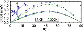
Figure 1: Data points and fits of $dF/d\theta$ calculated for GdCo₅ (blue, empty symbols; Gd and Co moments held antiparallel) and YCo₅ (green, filled symbols), at 0 and 300 K.

YCo₅ and GdCo₅ crystallize in the CaCu₅ structure, consisting of alternating hexagonal RCo_2c/Co_3g layers Kumar (1988). Y is nonmagnetic, while in GdCo₅ the large spin moment of Gd (originating mainly from its half-filled 4$f$ shell) aligns antiferromagnetically with the Co moments. We now consider a “standard” calculation of the MCA based on a rigid rotation of the magnetization. If the Gd and Co moments are held antiparallel, GdCo₅ is effectively a ferromagnet with reduced moment $M_{\mathrm{Co}}-M_{\mathrm{Gd}}$. Then, from the hexagonal symmetry we expect the angular dependence of the free energy to follow $\kappa_{1}\sin^{2}\theta+\kappa_{2}\sin^{4}\theta+\mathcal{O}(\sin^{6}\theta)$, where $\theta$ is the polar angle between the crystallographic $c$ axis and the magnetization direction. The constants $\kappa_{1},\kappa_{2}$ determine the change in free energy $\Delta F$, calculated e.g. from the force theorem Daalderop et al. (1990) or the torque $dF/d\theta$ Wang et al. (1996).

In Fig. 1 we show $dF/d\theta$ calculated for ferromagnetic YCo₅ and GdCo₅ at 0 and 300 K. Fitting the data to the derivative of the textbook expression, $\sin 2\theta(\kappa_{1}+2\kappa_{2}\sin^{2}\theta)$, finds $\kappa_{1}$ and $\kappa_{2}$ to be positive (easy $c$ axis) with $\kappa_{1}$ an order of magnitude larger than $\kappa_{2}$. Considering experimentally measured anisotropy constants in the literature, for YCo₅ our $\kappa_{1}$ value of 3.67 meV (all energies are per formula unit, f.u.) at 0 K compares favorably to the values of 3.6 and 3.9 meV reported in Refs. Yermolenko (1980) and Alameda et al. (1981). At 300 K, our value of 2.19 meV exhibits a slightly faster decay with temperature compared to experiment (2.6 and 3.0 meV), which we attribute to our use of a classical spin hamiltonian in the DLM picture Györffy et al. (1985); Patrick et al. (2017). However, for GdCo₅ our calculated values of $\kappa_{1}$ show very poor agreement with experiments Ermolenko (1976); Ballou et al. (1986). First, at 0 K we find $\kappa_{1}$ to be larger than YCo₅ (4.26 meV), while experimentally the anisotropy constant is much smaller (1.5, 2.1 meV). Second, we find $\kappa_{1}$ decreases with temperature (2.39 meV at 300 K) while experimentally the anisotropy constant increases (2.7, 2.8 meV).

To understand these discrepancies we must ask how the anisotropy energies were actually measured. Torque magnetometry provides an accurate method of accessing the MCA Klein et al. (1975), but is technically challenging in RE-TM magnets, which require very high fields to reach saturation Buschow and de Boer (2003). Singular point detection Paoluzi et al. (1994) and ferromagnetic resonance Wang et al. (2003) has also been used to investigate the MCA of polycrystalline and thin-film samples. However, the most commonly-used method for RE-TM magnets, employed in Refs. Ermolenko (1976); Ballou et al. (1986), is based on the seminal 1954 work by Sucksmith and Thompson Sucksmith and Thompson (1954) on the anisotropy of hexagonal ferromagnets. This work provides a relation between the measured magnetization $M_{\mathrm{ab}}$ and field $B$ applied in the hard plane in terms of $\kappa_{1}$, $\kappa_{2}$ and the easy axis magnetization $M_{0}$ Sucksmith and Thompson (1954); SM :

$$(BM_{0}/2)/\left(M_{\mathrm{ab}}/M_{0}\right)\equiv\eta=\kappa_{1}+2\kappa_{2}\left(M_{\mathrm{ab}}/M_{0}\right)^{2}.$$ (1)

Further introducing $m=(M_{\mathrm{ab}}/M_{0})$, equation 1 shows that a plot of $\eta$ against $m^{2}$ should yield a straight line with $\kappa_{1}$ as the intercept. Even though this “Sucksmith-Thompson method” was derived for ferromagnets, the technical procedure of plotting $\eta$ against $m^{2}$ can be performed also for ferrimagnets like GdCo₅ Ermolenko (1976); Ballou et al. (1986). In this case, the quantity extracted from the intercept is an effective anisotropy constant $K_{\mathrm{eff}}$ so, unlike YCo₅, the anisotropy constants reported in Refs. Ermolenko (1976); Ballou et al. (1986) are distinct from the $\kappa_{1}$ values extracted from Fig. 1. As recognized at the time of the original experiments Rinaldi and Pareti (1979); Yermolenko (1980); Ballou et al. (1986); Radwański (1986), the reduced value of $K_{\mathrm{eff}}$ with respect to $\kappa_{1}$ of YCo₅ is a fingerprint of canting between the Gd and Co sublattices.

Making contact with previous experiments thus requires we obtain $K_{\mathrm{eff}}$. To this end we have developed a scheme of calculating first-principles hard-plane magnetization vs. field (FPMVB) curves, on which we perform the Sucksmith-Thompson analysis to directly mirror the experiments. The central concept of FPMVB is that at equilibrium, the torques from the exchange, spin-orbit and dipole interactions must balance those arising from the external field. Then,

$$B=\frac{\partial F(T)}{\partial\theta_{i}}\frac{1}{M_{i}\cos\theta_{i}+\sum_{j}\sin\theta_{j}\frac{\partial M_{j}}{\partial\theta_{i}}}.$$ (2)

The magnetization at a given $B,T$ is determined by the angle set $\{\theta_{\mathrm{Gd}},\theta_{\mathrm{Co_{1}}},\theta_{\mathrm{Co_{2}}},...\}$ which satisfies equation 2 for every magnetic sublattice. The spin-orbit interaction breaks the symmetry of the Co_3g atoms such that altogether there are four independent angles to vary for GdCo₅. The second term in the denominator of equation 2 reflects that the magnetic moments themselves might depend on $\theta_{i}$ (magnetization anisotropy). We have tested (i) neglecting this contribution and (ii) modeling the dependence as $M_{i}(\theta_{i})=M_{0i}(1-p_{i}\sin^{2}\theta_{i})$, where $M_{0i}$ and $p_{i}$ are parameterized from our calculations.

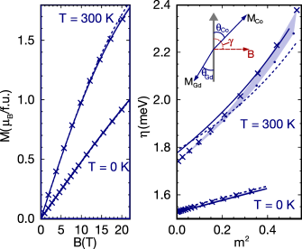
Figure 2: Magnetization of GdCo₅ vs. applied magnetic field shown on a standard plot (left panel) or after the Sucksmith-Thompson analysis (eq. 1, right panel). Crosses/circles are calculated with methods (i)/(ii) discussed in the text, and the area between them shaded as a guide to the eye. Note the two methods are effectively indistinguishable in the left panel. The dashed/solid lines are calculated from the model free energies $F_{1}$ and $F_{2}$. The right panel also shows the geometry of the magnetization and field with respect to the crystallographic $c$-axis (thick gray arrow).

Figure 2 shows FPMVB curves of GdCo₅ calculated using equation 2 with methods (i) and (ii), (crosses and circles) which yield virtually identical values of $K_{\mathrm{eff}}$. The $M$ vs. $B$ curves in the left panel resemble those of a ferromagnet where, as the temperature increases, it becomes easier to rotate the moments away from the easy axis so that a given $B$ field induces a larger magnetization. However, plotting $\eta$ against $m^{2}$ in the right panel tells a more interesting story. The effective anisotropy constant $K_{\mathrm{eff}}$ ($y$-axis intercept) at 0 K is 1.53 meV, much smaller than $\kappa_{1}$ of YCo₅. Furthermore $K_{\mathrm{eff}}$ increases with temperature, to 1.74 meV at 300 K. Therefore, in contrast to the standard calculations of Fig. 1, the FPMVB approach reproduces the experimental behavior of Refs. Ermolenko (1976); Ballou et al. (1986).

Our FPMVB calculations provide a microscopic insight into the magnetization process. For instance at 0 K and 9 T, we calculate that the cobalt moments rotate away from the easy axis by 6.1^∘. By contrast the Gd moments have rotated by only 3.9^∘, i.e. the ideal 180^∘ Gd-Co alignment has reduced by 2.2^∘ (the geometry is shown in Fig. 2). We also find canting between the different Co sublattices, but not by more than 0.1^∘ at both 0 and 300 K (the calculated angles as a function of field are shown in the SM SM ). This Co-Co canting is small thanks to the Co-Co ferromagnetic exchange interaction, which remains strong over a wide temperature range Patrick et al. (2017). The temperature dependence of $K_{\mathrm{eff}}$ can be traced to the fact that the easy axis magnetization $M_{0}$ of GdCo₅ initially increases with temperature Patrick et al. (2017). Even if $M_{\mathrm{ab}}$ increases with temperature at a given field, a faster increase in $M_{0}$ can lead to an overall hardening in $K_{\mathrm{eff}}$ (equation 1).

We assign the canting in GdCo₅ to a delicate competition between the exchange interaction favoring antiparallel Co/Gd moments, uniaxial anisotropy favoring $c$-axis (anti)alignment, and the external field trying to rotate all moments into the hard plane. We can quantify these interactions by looking for a model parameterization of the free energy $F$. Crucially we can train the model with an arbitrarily large set of first-principles calculations exploring sublattice orientations not accessible experimentally, and test its performance against the torque calculations of equation 2. Neglecting the 0.1^∘ canting within the cobalt sublattices gives two free angles, $\theta_{\mathrm{Gd}}$ and $\theta_{\mathrm{Co}}$. Including Gd-Co exchange $A$, uniaxial Co anisotropy $K_{\mathrm{1,Co}}$ and a dipolar contribution $S(\theta_{\mathrm{Gd}},\theta_{\mathrm{Co}})$ Ballou et al. (1987); SM leads naturally to a two-sublattice model Radwański (1986),

$$F_{1}(\theta_{\mathrm{Gd}},\theta_{\mathrm{Co}}) = -A\cos(\theta_{\mathrm{Gd}}-\theta_{\mathrm{Co}})+K_{\mathrm{1,Co}}\sin^{2}\theta_{\mathrm{Co}}$$ (3)

$$+S(\theta_{\mathrm{Gd}},\theta_{\mathrm{Co}}).$$

The training calculations showed additional angular dependences not captured by $F_{1}$, so we also investigated:

$$F_{2}(\theta_{\mathrm{Gd}},\theta_{\mathrm{Co}}) = F_{1}(\theta_{\mathrm{Gd}},\theta_{\mathrm{Co}})+K_{\mathrm{2,Co}}\sin^{4}\theta_{\mathrm{Co}}$$ (4)

$$+K_{\mathrm{1,Gd}}\sin^{2}\theta_{\mathrm{Gd}}.$$

As discussed below the training calculations showed no strong evidence of Gd-Co exchange anisotropy Ballou et al. (1987); Gerard and Ballou (1992); Radwański et al. (1992); Franse and Radwański (1993).

The dashed (solid) lines in Fig. 2 are the calculated $M$ vs. $B$ curves obtained by minimizing $F_{1(2)}-\sum_{i}\bm{M_{i}}\cdot\bm{B}$. The second term includes magnetization anisotropy on the cobalt moments SM ; Alameda et al. (1980). On the scale of the left panel both $F_{1}$ and $F_{2}$ give excellent fits to the torque calculations, especially up to moderate fields. The plot of $\eta$ against $m^{2}$ reveals some differences with $F_{2}$ giving a marginally improved description of the data, but $F_{1}$ already captures the most important physics.

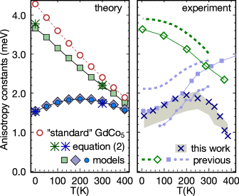
Figure 3: Anisotropy constants $K_{\mathrm{eff}}$ vs. temperature of YCo₅ (green) and GdCo₅ (blue). The left panel shows calculations using equation 2 at 0 and 300 K (stars), or using parameterized model expressions $F_{1}$ (diamonds) and $F_{2}$ (circles), and from Ref. Alameda et al. (1980) (YCo₅, squares). For GdCo₅ we also show in red $\kappa_{1}$ extracted from “standard” calculations where the Gd and Co moments were held rigidly antiparallel (cf. Fig. 1). The experimental data in the right panel was measured by us for GdCo₅ (crosses, with shaded background) or taken from Refs. Ermolenko (1976), Ballou et al. (1986) and Katayama et al. (1976) (squares, dashed lines, circles) and Refs Yermolenko (1980) and Alameda et al. (1981) (green diamonds and dashed lines, YCo₅).

We also applied the FPMVB approach to YCo₅, using equation 2 and the model for $F$ introduced in Ref. Alameda et al. (1980). Then, parameterizing the models SM over the temperature range 0–400 K, calculating $M$ vs. $B$ curves and extracting $K_{\mathrm{eff}}$ using the Sucksmith-Thompson plots gives the results shown in the left panel of Fig. 3. We also show $\kappa_{1}$ of GdCo₅ to emphasize the difference between FPMVB calculations and the “standard” ones of Fig. 1.

Comparing $K_{\mathrm{eff}}$ to previously-published experimental measurements on GdCo₅ raises some issues. First, the three studies in the literature report anisotropy constants which differ by as much as 1 meV Ermolenko (1976); Ballou et al. (1986); Katayama et al. (1976). Indeed there was controversy over whether the observed results were evidence of an anisotropic exchange interaction between Gd and Co Ballou et al. (1987); Gerard and Ballou (1992) or an artefact of poor sample stoichiometry Radwański et al. (1992); Franse and Radwański (1993). Furthermore the only study performed above room temperature Ermolenko (1976) reports without comment some peculiar behavior where $K_{\mathrm{eff}}$ of GdCo₅ exceeds that of YCo₅ at high temperature Yermolenko (1980), despite conventional wisdom that the half-filled $4f$ shell of Gd does not contribute to the anisotropy.

Our calculations do in fact show an excess in the rigid-moment anisotropy of GdCo₅ of 16% at 0 K (Fig. 1) compared to YCo₅. The authors of Refs. Ballou et al. (1986, 1987) fitted their experimental data with a much larger excess of 50%, while the high-field study of Ref. Radwański et al. (1992) found (11 $\pm$ 15)%, with the authors of that work attributing the difference to an improved sample stoichiometry Franse and Radwański (1993). Our calculated excess at 0 K is formed from two major contributions: the dipole interaction energy, which accounts for 0.31 meV/f.u., and $K_{1,\mathrm{Gd}}$ (equation 4) which we found to be 24% the size of $K_{1,\mathrm{Co}}$. The nonzero value of $K_{1,\mathrm{Gd}}$ is due to the 5$d$ electrons, whose presence is evident from the Gd magnetization (7.47$\mu_{B}$ at 0 K). We did not find a significant contribution from anisotropic exchange, which we tested in two ways: first by attempting to fit a term $A(1-p^{\prime}\sin^{2}\theta_{\mathrm{Co}})\cos(\theta_{\mathrm{Gd}}-\theta_{\mathrm{Co}})$ to our training set of calculations, and also by computing Curie temperatures with the (rigidly antiparallel) magnetization directed either along the $c$ or $a$ axes. We found the magnitude of the anisotropy ($p^{\prime}$) to be smaller than 0.5% and negative at 0 K, and to decrease in magnitude as the temperature is raised. Consistently the Curie temperature was found to be only 1 K higher for $a$ axis alignment, which we do not consider significant.

However, our calculations do not predict the $K_{\mathrm{eff}}$ value of GdCo₅ to exceed YCo₅. Indeed, in Fig. 3 $\kappa_{1}$ of GdCo₅ approaches that of YCo₅ at high temperatures, which is significant because $\kappa_{1}$ provides an upper bound for $K_{\mathrm{eff}}$ Gerard and Ballou (1992). To resolve this final puzzle we performed our own measurements of $K_{\mathrm{eff}}$ on the single crystal whose growth we reported recently Patrick et al. (2017). Hard and easy axis magnetization curves up to 7 T were measured in a Quantum Design superconducting quantum interference device (SQUID) magnetometer, and the anisotropy constants extracted from Sucksmith-Thompson plots SM . The right panel of Fig. 3 shows our newly measured data as crosses. Previously reported measurements are shown in faint blue/green for GdCo₅ Ermolenko (1976); Ballou et al. (1986); Katayama et al. (1976)/YCo₅ Alameda et al. (1981); Yermolenko (1980).

Up to 200 K, there is close agreement between the experiments of Ref. Ermolenko (1976), our own experiments, and the FPMVB calculations. Above this temperature our new experiments show the expected drop in $K_{\mathrm{eff}}$, while the previously reported data show a continued rise Ermolenko (1976). We repeated our measurements using different protocols and found a reasonably large variation in the extracted $K_{\mathrm{eff}}$ SM . Even taking this variation into account as the shaded area in Fig. 3, the drop is still observed.

We therefore do not believe the high temperature behavior reported in Ref. Ermolenko (1976) has an intrinsic origin. Possible extrinsic factors include the method of sample preparation, degradation of the RCo₅ phase at elevated temperatures Den Broeder and Buschow (1972), and potential systematic error when extracting $K_{\mathrm{eff}}$. We note that even the idealized theoretical curves in Fig. 2 show curvature at higher temperature, making it more difficult to find the intercept.

In conclusion, we have introduced the FPMVB approach to interpret experiments measuring anisotropy of ferrimagnets, particularly RE-TM permanent magnets. We presented the method in the context of our DLM formalism, but any electronic structure theory capable of calculating magnetic couplings relativistically Udvardi et al. (2003); Ebert and Mankovsky (2009); Hu and Wu (2013); Ayaz Khan et al. (2016); Hoffmann et al. (2017) should be able to produce FPMVB curves, at least at zero temperature. However standard calculations which neglect the external field should be used with care when comparing to experiments on ferrimagnets. Similarly, the prototype GdCo₅ serves as a reminder that a simple view of the anisotropy energy does not fully describe the magnetization processes in ferrimagnets, which might have implications in understanding e.g.  magnetization reversal in nano-magnetic assemblies Guo et al. (2002). Overall our work demonstrates the benefit of interconnected computational and experimental research in this key area.

The present work forms part of the PRETAMAG project, funded by the UK Engineering and Physical Sciences Research Council (EPSRC), Grant no.  EP/M028941/1. Crystal growth work at Warwick is also supported by EPSRC Grant no. EP/M028771/1. Work at Daresbury Laboratory was supported by an EPSRC service level agreement with the Scientific Computing Department of STFC. We thank E. Mendive-Tapia for useful discussions and A. Vasylenko for continued assistance in translating references.

References

- Chikazumi (1997) S. Chikazumi, Physics of Ferromagnetism, 2nd ed. (Oxford University Press, 1997).
- Kronmüller (1987) H. Kronmüller, Phys. Stat. Sol. b 144, 385 (1987).
- Strange (1998) P. Strange, Relativistic Quantum Mechanics (Cambridge University Press, 1998).
- Strnat et al. (1967) K. Strnat, G. Hoffer, J. Olson, W. Ostertag, and J. J. Becker, J. Appl. Phys. 38, 1001 (1967).
- Gutfleisch et al. (2011) O. Gutfleisch, M. A. Willard, E. Brück, C. H. Chen, S. G. Sankar, and J. P. Liu, Adv. Mater. 23, 821 (2011).
- Sagawa et al. (1984) M. Sagawa, S. Fujimura, N. Togawa, H. Yamamoto, and Y. Matsuura, J. Appl. Phys. 55, 2083 (1984).
- Croat et al. (1984) J. J. Croat, J. F. Herbst, R. W. Lee, and F. E. Pinkerton, J. Appl. Phys. 55, 2078 (1984).
- Coey (2011) J. M. D. Coey, IEEE Trans. Magn. 47, 4671 (2011).
- Skomski et al. (2013) R. Skomski, P. Manchanda, P. Kumar, B. Balamurugan, A. Kashyap, and D. J. Sellmyer, IEEE Trans. Magn. 49, 3215 (2013).
- Kuz’min and Tishin (2008) M. D. Kuz’min and A. M. Tishin, in Handbook of Magnetic Materials, Vol. 17, edited by K. H. J. Buschow (Elsevier B.V., 2008) Chap. 3, p. 149.
- Tie-song et al. (1991) Z. Tie-song, J. Han-min, G. Guang-hua, H. Xiu-feng, and C. Hong, Phys. Rev. B 43, 8593 (1991).
- Richter (1998) M. Richter, J. Phys. D: Appl. Phys. 31, 1017 (1998).
- Kuz’min et al. (2004) M. D. Kuz’min, Y. Skourski, D. Eckert, M. Richter, K.-H. Müller, K. P. Skokov, and I. S. Tereshina, Phys. Rev. B 70, 172412 (2004).
- Delange et al. (2017) P. Delange, S. Biermann, T. Miyake, and L. Pourovskii, Phys. Rev. B 96, 155132 (2017).
- Steinbeck et al. (2001a) L. Steinbeck, M. Richter, and H. Eschrig, J. Magn. Magn. Mater. 226–230, Part 1, 1011 (2001a).
- Larson et al. (2004) P. Larson, I. I. Mazin, and D. A. Papaconstantopoulos, Phys. Rev. B 69, 134408 (2004).
- Pang et al. (2009) H. Pang, L. Qiao, and F. S. Li, Phys. Status Solidi B 246, 1345 (2009).
- Matsumoto et al. (2014) M. Matsumoto, R. Banerjee, and J. B. Staunton, Phys. Rev. B 90, 054421 (2014).
- Landa et al. (2017) A. Landa, P. Söderlind, D. Parker, D. Åberg, V. Lordi, A. Perron, P. E. A. Turchi, R. K. Chouhan, D. Paudyal, and T. A. Lograsso, “Thermodynamics of the SmCo5 compound doped with Fe and Ni: an ab initio study,” (2017), arXiv:1707.09447 .
- Eriksson et al. (1990) O. Eriksson, B. Johansson, R. C. Albers, A. M. Boring, and M. S. S. Brooks, Phys. Rev. B 42, 2707 (1990).
- Eschrig et al. (2005) H. Eschrig, M. Sargolzaei, K. Koepernik, and M. Richter, Europhys. Lett. 72, 611 (2005).
- Daalderop et al. (1996) G. H. O. Daalderop, P. J. Kelly, and M. F. H. Schuurmans, Phys. Rev. B 53, 14415 (1996).
- Staunton et al. (2004) J. B. Staunton, S. Ostanin, S. S. A. Razee, B. L. Gyorffy, L. Szunyogh, B. Ginatempo, and E. Bruno, Phys. Rev. Lett. 93, 257204 (2004).
- Kumar (1988) K. Kumar, J. Appl. Phys. 63, R13 (1988).
- Buschow et al. (1974) K. Buschow, A. van Diepen, and H. de Wijn, Solid State Commun. 15, 903 (1974).
- Ermolenko (1976) A. Ermolenko, IEEE Trans. Mag. 12, 992 (1976).
- Rinaldi and Pareti (1979) S. Rinaldi and L. Pareti, J. Appl. Phys. 50, 7719 (1979).
- Yermolenko (1980) A. S. Yermolenko, Fiz. Metal. Metalloved. 50, 741 (1980).
- Ballou et al. (1986) R. Ballou, J. Déportes, B. Gorges, R. Lemaire, and J. Ousset, J. Magn. Magn. Mater. 54, 465 (1986).
- Radwański (1986) R. Radwański, Physica B+C 142, 57 (1986).
- Ballou et al. (1987) R. Ballou, J. Déportes, and J. Lemaire, J. Magn. Magn. Mater. 70, 306 (1987).
- Gerard and Ballou (1992) P. Gerard and R. Ballou, J. Magn. Magn. Mater. 104, 1463 (1992).
- Radwański et al. (1992) R. Radwański, J. Franse, P. Quang, and F. Kayzel, J. Magn. Magn. Mater. 104, 1321 (1992).
- Franse and Radwański (1993) J. J. M. Franse and R. J. Radwański, in Handbook of Magnetic Materials, Vol. 7, edited by K. H. J. Buschow (Elsevier North-Holland, New York, 1993) Chap. 5, p. 307.
- Zhao et al. (1991) T. Zhao, H. Jin, R. Grössinger, X. Kou, and H. R. Kirchmayr, J. Appl. Phys. 70, 6134 (1991).
- Györffy et al. (1985) B. L. Györffy, A. J. Pindor, J. Staunton, G. M. Stocks, and H. Winter, J. Phys. F: Met. Phys. 15, 1337 (1985).
- Staunton et al. (2006) J. B. Staunton, L. Szunyogh, A. Buruzs, B. L. Gyorffy, S. Ostanin, and L. Udvardi, Phys. Rev. B 74, 144411 (2006).
- Note (1) We performed a sum over dipoles Chikazumi (1997) using the calculated out to a radius of 20 nm.
- Bruno and Ginatempo (1997) E. Bruno and B. Ginatempo, Phys. Rev. B 55, 12946 (1997).
- Strange et al. (1984) P. Strange, J. Staunton, and B. L. Gyorffy, J. Phys. C: Solid State Phys. 17, 3355 (1984).
- Däne et al. (2009) M. Däne, M. Lüders, A. Ernst, D. Ködderitzsch, W. M. Temmerman, Z. Szotek, and W. Hergert, J. Phys.: Condens. Matter 21, 045604 (2009).
- Vosko et al. (1980) S. H. Vosko, L. Wilk, and M. Nusair, Can. J. Phys. 58, 1200 (1980).
- Lüders et al. (2005) M. Lüders, A. Ernst, M. Däne, Z. Szotek, A. Svane, D. Ködderitzsch, W. Hergert, B. L. Györffy, and W. M. Temmerman, Phys. Rev. B 71, 205109 (2005).
- Patrick et al. (2017) C. E. Patrick, S. Kumar, G. Balakrishnan, R. S. Edwards, M. R. Lees, E. Mendive-Tapia, L. Petit, and J. B. Staunton, Phys. Rev. Materials 1, 024411 (2017).
- Ebert and Battocletti (1996) H. Ebert and M. Battocletti, Solid State Commun. 98, 785 (1996).
- Ebert (2000) H. Ebert, “Fully relativistic band structure calculations for magnetic solids - formalism and application,” in Electronic Structure and Physical Properies of Solids: The Uses of the LMTO Method Lectures of a Workshop Held at Mont Saint Odile, France, October 2–5,1998, edited by H. Dreyssé (Springer Berlin Heidelberg, Berlin, Heidelberg, 2000) pp. 191–246.
- Steinbeck et al. (2001b) L. Steinbeck, M. Richter, and H. Eschrig, Phys. Rev. B 63, 184431 (2001b).
- (48) See Supplemental Material for further experimental and computational details, description of the orbital polarization correction, discussion of magnetization anisotropy, the parameters used to simulate curves and the angle sets which satisfy equation 2.
- Daalderop et al. (1990) G. H. O. Daalderop, P. J. Kelly, and M. F. H. Schuurmans, Phys. Rev. B 41, 11919 (1990).
- Wang et al. (1996) X. Wang, R. Wu, D.-s. Wang, and A. J. Freeman, Phys. Rev. B 54, 61 (1996).
- Alameda et al. (1981) J. M. Alameda, D. Givord, R. Lemaire, and Q. Lu, J. Appl. Phys. 52, 2079 (1981).
- Klein et al. (1975) H. Klein, A. Menth, and R. Perkins, Physica B+C 80, 153 (1975).
- Buschow and de Boer (2003) K. H. J. Buschow and F. R. de Boer, Physics of Magnetism and Magnetic Materials (Springer, Boston, MA, 2003).
- Paoluzi et al. (1994) A. Paoluzi, L. Pareti, M. Solzi, and F. Albertini, J. Magn. Magn. Mater. 132, 185 (1994).
- Wang et al. (2003) Y. Wang, Y. Zhao, S. Wang, M. Lu, H. Zhai, Y. Zhai, K. Shono, and X. Yu, J. Appl. Phys. 93, 7789 (2003).
- Sucksmith and Thompson (1954) W. Sucksmith and J. E. Thompson, Proc. Royal Soc. A 225, 362 (1954).
- Alameda et al. (1980) J. Alameda, J. Déportes, D. Givord, R. Lemaire, and Q. Lu, J. Magn. Magn. Mater. 15, 1257 (1980).
- Katayama et al. (1976) T. Katayama, M. Ohkoshi, Y. Koizumi, T. Shibata, and T. Tsushima, Appl. Phys. Lett. 28, 635 (1976).
- Den Broeder and Buschow (1972) F. Den Broeder and K. Buschow, J. Less-Common Metals 29, 65 (1972).
- Udvardi et al. (2003) L. Udvardi, L. Szunyogh, K. Palotás, and P. Weinberger, Phys. Rev. B 68, 104436 (2003).
- Ebert and Mankovsky (2009) H. Ebert and S. Mankovsky, Phys. Rev. B 79, 045209 (2009).
- Hu and Wu (2013) J. Hu and R. Wu, Phys. Rev. Lett. 110, 097202 (2013).
- Ayaz Khan et al. (2016) S. Ayaz Khan, P. Blaha, H. Ebert, J. Minár, and O. Šipr, Phys. Rev. B 94, 144436 (2016).
- Hoffmann et al. (2017) M. Hoffmann, B. Zimmermann, G. P. Müller, D. Schürhoff, N. S. Kiselev, C. Melcher, and S. Blügel, Nat. Commun. 8, 308 (2017).
- Guo et al. (2002) Z. J. Guo, J. S. Jiang, J. E. Pearson, S. D. Bader, and J. P. Liu, Appl. Phys. Lett. 81, 2029 (2002).