Identifying Young $Kepler$ Planet Host Stars from Keck-HIRES Spectra of Lithium

Abstract

The lithium doublet at 6708 Å provides an age diagnostic for main sequence FGK dwarfs. We measured the abundance of lithium in 1305 stars with detected transiting planets from the Kepler Mission using high-resolution spectroscopy. Our catalog of lithium measurements from this sample have a range of abundance from A(Li) = 3.11 $\pm$ 0.07 to an upper limit of $-$0.84 dex. For a magnitude-limited sample that comprises 960 of the 1305 stars, our Keck-HIRES spectra have a median S/N = 45 per pixel at $\sim$6700 Å with spectral resolution $\frac{\lambda}{\Delta\lambda}$ = $R$ = 55,000. We identify 80 young stars that have A(Li) values greater than the Hyades at their respective effective temperatures; these stars are younger than $\sim$650 Myr old, the approximate age of the Hyades. We then compare the distribution of A(Li) with planet size, multiplicity, orbital period, and insolation flux. We find larger planets preferentially in younger systems, with an A-D two-sided test p-value = 0.002, a $>3\sigma$ confidence that the older and younger planet samples do not come from the same parent distribution. This is consistent with planet inflation/photoevaporation at early ages. The other planet parameters ($Kepler$ planet multiplicity, orbital period, and insolation flux) are uncorrelated with age.

1 Introduction

NASA’s $Kepler$ Mission was designed to detect transiting planets and to measure the fraction of Sun-like stars with Earth-sized planets in the habitable zone. During the four year mission, $Kepler$ discovered more than 4000 exoplanet candidates, of which 2327 have been confirmed (Coughlin et al. 2016). Twenty-one of these confirmed exoplanets are 1–2$\times$ Earth size and orbit in the traditionally defined habitable zone. Analysis of $Kepler$ data demonstrated that 50% of Sun-like stars harbor a planet between the size of Earth and Neptune with orbital periods less than 85 days (Fressin et al. 2013). Complementary Doppler surveys of nearby stars showed that 8.5% of giant planets with periods shorter than a few years orbit similar type stars (Cumming et al. 2008). Studies by Howard et al. (2010), Mayor et al. (2011), and Howard et al. (2012) have shown that giant planets are less plentiful than their smaller counterparts. In addition, $Kepler$ analysis uncovered a diverse set of exoplanetary systems, some of which have peculiar properties and architectures. Noteworthy systems include the two habitable zone planets orbiting $Kepler$-62 (Borucki et al. 2013), the Earth-size planet with an 8.5 hour period orbiting $Kepler$-78 (Sanchis-Ojeda et al. 2013), and the $Kepler$-47 circumbinary system (Orosz et al. 2012). In each of these cases, measuring the stellar properties (e.g., radii, masses, and effective temperatures) is critical to determine the planet properties. For instance, all transit-derived planet radii scale directly with the stellar radius. Among the stellar properties, age is frequently unknown or poorly determined. Age is important because dynamic processes including mass loss, contraction, reinflation, and migration sculpt the planet population that we observe today.

Accurately determining stellar ages is difficult. The precise age of 4.567 Gyr for the sun is based on isotopic measurements of meteorites (Chaussidon 2007), a method that is unavailable for other stars. Soderblom (2010) provides a comprehensive review of the techniques to determine approximate stellar ages, including (1) kinematics, (2) isochrone placement through measured temperature, metallicity, and luminosity, (3) asteroseismology, (4) rotation rate, (5) magnetic activity, (6) lithium abundance, and (7) nucleocosmochronometry.

Some of these methods are based on only a few assumptions, but are observationally demanding. For example, nucleocosmochronometry requires high-resolution, high-signal-to-noise spectra and kinematic techniques need large groups of stars. Isochrone placement using precise temperatures, metallicity, and luminosity (together with their uncertainties) and asteroseismology are model-dependent methods that rely on detailed stellar physics. Sometimes, even with high quality observational data, astronomers cannot determine an isochrone age for stars using either method, due to poor interpolation between models and unresolved degeneracies in the Hertzprung-Russell Diagram. Empirical methods involving stellar rotation and magnetic activity are limited by calibration, measurement precision, and intrinsic astrophysical variability.

Surface lithium abundance provides another age diagnostic. Herbig (1965) was one of the first to consider Li as an age diagnostic for F and G stars. As Li is destroyed in the stellar interior at temperatures of $2.5\times 10^{6}$ K primarily by ($p$,$\alpha$) reactions, surface Li abundance declines with time. The rate of decline is not uniform because transport mechanisms including convection and gravitational settling depend on effective temperature (Xiong & Deng 2009). Lithium abundance can be measured by using the resonance doublet at 6708 Å of Li I in stars. Measuring Li is observationally convenient because our high-resolution optical spectra used to determine bulk parameters ($T_{\mathrm{eff}}$, $\log g$, [Fe/H]) include the Li feature. Additionally, Li ages have been calibrated with measurements of several clusters. Unfortunately, precise ages are difficult to establish from sole analysis of the Li feature, but its presence is a discriminator of youth at least.

Others, such as Israelian et al. (2009), Baumann et al. (2010), Sousa et al. (2010), Ramírez et al. (2012), Delgado Mena et al. (2014, 2015), Figueira et al. (2014), and Gonzalez (2014, 2015), have compared stellar Li abundance for exoplanet hosts versus single stars. Israelian et al. (2009) studied a uniform sample of 451 stars in the HARPS high precision radial velocity survey, with stars spanning $T_{\mathrm{eff}}$ = 4900–6500 K. The authors found low Li abundance (A(Li) $\equiv$ 12 + $\log(\mathrm{Li/H})$) for stars in a narrow temperature range ($T_{\mathrm{eff}}$ = 5700–5850 K) compared to stars without exoplanet companions, while excluding metallicity, age, $v\sin{i}$, and activity as possible causes for this anomaly. They hypothesized mechanisms to account for this trend: stars with planets might experience a) a different evolution, b) planets might infall and cause stellar mixing, and c) there may be interaction during the pre-main sequence (PMS) phase which can force high differential rotation and therefore enhanced Li depletion within planet-host stars.

However, some more recent work (Baumann et al. 2010; Ramírez et al. 2012) contradicted the results of Israelian et al. (2009), while others (Sousa et al. 2010; Delgado Mena et al. 2014, 2015; Figueira et al. 2014; Gonzalez 2014, 2015) found supporting evidence for enhanced host star Li depletion. Baumann et al. (2010) studied a sample of 117 solar-type stars, 14 of which were planet-hosts. These stars exhibited normal A(Li) for their ages. In addition, the authors showed that 82 stars originally reported in the literature to support enhanced Li depletion in fact had normal A(Li) for their ages. Baumann et al. (2010) provide a few reasons for the disagreement between their results and Israelian et al. (2009): (1) the HARPS sample of solar analogs at [Fe/H] $\simeq$ 0.0 are on average older than non-planet-host stars, (2) metal-rich solar analogs are more lithium-poor than solar metallicity stars, and (3) the sample includes a number of peculiarly high Li abundances.

Ramírez et al. (2012), like Baumann et al. (2010), found that any connection between Li abundance and planet occurrence is likely a product of sample bias in stellar mass, age, and metallicity. Ramírez et al. (2012) studied a sample of 1381 dwarf and subgiant stars, 165 of which were planet-hosts. The large sample size allowed them to analyze trends in A(Li) with the presence of exoplanets, but the planet hosts and non-hosts were taken from different sources, and therefore could suffer from inhomogeneities. Their data suggest there is some planet-star interaction (not necessarily planet formation-related) that prevents planet-host stars from experiencing the sudden drop in A(Li) responsible for the Li desert, a region in A(Li)-$T_{\mathrm{eff}}$ space where stars should appear empirically, but do not. Ultimately, Ramírez et al. (2012) rejected the presence of enhanced Li depletion in planet-hosts proposed by Israelian et al. (2009) after claiming to properly account for all possible sources of bias.

Unlike Baumann et al. (2010) and Ramírez et al. (2012), a number of other studies continued to find enhanced Li depletion in host stars (Sousa et al. 2010; Delgado Mena et al. 2014, 2015; Figueira et al. 2014; Gonzalez 2014, 2015). Sousa et al. (2010) investigated potential effects of age and mass on Li depletion and found that differences in ages and stellar mass could not explain the Li deficit in planet host stars. Gonzalez (2014, 2015) introduced new high resolution spectra of late-F and early-G stars, determined A(Li), and then added homogeneous literature data, finding that Li is deficient in giant planet hosts compared to comparison stars.

Delgado Mena et al. (2014) focused again on solar-type stars, finding that solar twins with hot jupiters show enhanced Li depletion compared to those without planets. In contrast to Ramírez et al. (2012), Delgado Mena et al. (2014) utilized a homogeneous sample, entirely from HARPS and including both stars with planets and those without, to minimize potential confounding effects in A(Li). Figueira et al. (2014) used multivariable regression to test these confounding effects on previously published A(Li), and found that, when one assumes linearity in the fundamental stellar parameters, an offset in A(Li) between hosts and non-hosts is recovered. This offset is strongly statistically significant, but it is reduced to zero if host stars are replaced with comparison stars.

Finally, Delgado Mena et al. (2015) found a similar trend of Li depletion in late-F stars ($T_{\mathrm{eff}}$ = 5900–6300 K), although the differences in A(Li) between hosts and stars with no detected planets are smaller in magnitude than for solar-type stars. However, the authors found that hot jupiter hosts had a higher average $v\sin{i}$ than the comparison stars, so the enhanced Li depletion could be explained by rotationally-induced mixing and not the presence of planets. Given the studies following Ramírez et al. (2012) and the care taken to minimize contamination in the HARPS sample, the observational evidence for decreased Li in giant planet hosts is convincing.

No study has yet used A(Li) to differentiate between a large sample of young and old exoplanetary systems. Therefore, we present the first large scale (N $>$ 1000) study of Li in $Kepler$ planet host stars that separates the population into young and old age groups. This allows us to investigate planetary evolution and the dynamic processes (migration, mass loss, contraction, reinflation, etc.) that sculpt the observed planet population. Moreover, this analysis adds another impactful dimension to the current parameter space of exoplanets heavily characterized by mass, radius, and effective temperature.

In Section 2, we discuss the California-Kepler Survey sample. Section 3 details our pipeline to determine A(Li) and each of the important tasks performed therein, including normalization, Doppler shifting, measurement of the equivalent width of Li, and the A(Li) computation. Section 4 analyzes the full catalog and searches for any trends in exoplanetary parameters with age. In Section 5, we discuss our results and provide an astrophysical interpretation of our findings.

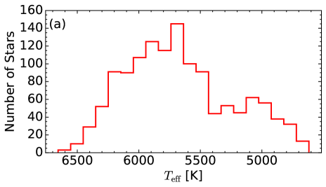
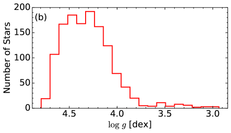
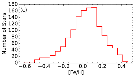
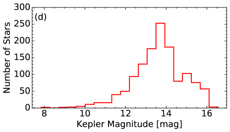
Figure 1: Stellar sample. $(a)$: Histogram showing $T_{\mathrm{eff}}$ for the 1305 CKS stars. $(b)$: Histogram of $\log g$ for the CKS sample. $(c)$: [Fe/H]. $(d)$: Distribution of Kepler magnitudes. The majority of the stars have KepMag $\lesssim$ 14.23 mag.

2 Stellar Sample

One key follow-up survey of $Kepler$-discovered exoplanets is the California Kepler Survey (CKS) (Petigura et al. 2017), which was proposed to measure precise stellar parameters ($T_{\mathrm{eff}}$, $\log g$, [Fe/H], $v\sin{i}$) by using local thermodynamic equilibrium (LTE) modeling of Keck-HIRES spectra of $\sim$1000 $Kepler$ FGK stars. Most of these stars are main sequence G and K dwarfs, but there are a few F stars. Figure 1 shows the distribution of our sample in $T_{\mathrm{eff}}$, $\log g$, and [Fe/H] histograms in plots (a), (b), and (c), respectively. The apparent magnitudes of the stars go down to 17th magnitude. Most spectra have signal-to-noise ratios ($S/N$) of $\sim$45 per pixel, or $\sim$90 per resolution element at 6700 Å, with a resolution $R$ = 55,000 and wavelength coverage from 3642–7990 Å. $S/N$ range from $\sim$5 to $\sim$200. We note that the primary CKS sample is magnitude-limited to a $Kepler$ magnitude (KepMag) $\lesssim$ 14.23 mag, with additional fainter stars from interesting groups, $i.e.$ habitable zone candidates and multi-planet systems. See Figure 1 plot (d) for the distribution of $Kepler$ magnitudes.

The spectra were reduced by removing cosmic rays, flat-fielding, bias subtraction, trimming, and column collapsing into a 1-D spectrum. We adopt the spectroscopic parameters ($T_{\mathrm{eff}}$, $\log g$, [Fe/H], $v\sin{i}$) from Petigura et al. (2017), computed from SpecMatch (Petigura 2015) and Spectroscopy Made Easy (Valenti & Piskunov 2012). The spectral format of HIRES was kept fixed with 1–2 pixel accuracy for all spectra.

3 Lithium Abundance Measurements

We begin with the reduced HIRES spectra from Petigura et al. (2017) as detailed in the previous paragraph. To efficiently determine Li abundances for all stars within the CKS sample, we created an automated Li pipeline, which we detail below. The pipeline’s spectrum analysis tasks include continuum normalization, Doppler correction, measurement of the Li equivalent width (EW), interpolation of a model atmosphere, determination of A(Li), and calculation of uncertainties ($\sigma_{\mathrm{A(Li)}}$).

3.1 Continuum Normalization and Doppler Correction

First, we utilized PyRAF’s $continuum$ routine to remove the blaze function present in every spectrum. We applied this technique with the following options: a 50-piece cubic spline fit, a low rejection criterion of 2.0$\sigma$, a high rejection criterion of 3.0$\sigma$, and 50 outlier rejection iterations. The output (normalized) spectrum is the input spectrum divided by the continuum-fit spline function. Outlier rejection allows $continuum$ to ignore any biasing effects from peaks (remaining cosmic rays) and troughs (absorption lines).

Next, we applied a Doppler correction to shift the spectrum into its rest frame. We determined the Doppler correction velocity by cross-correlating the rest-wavelength, National Solar Observatory (NSO) solar spectrum with the object spectrum. The NSO spectrum is an extremely high resolution and high $S/N$ solar spectrum collected with the Brault National Solar Observatory Fourier Transform Spectrometer (Wallace et al. 2011). Many of the same absorption lines appear in the solar and HIRES spectra due to the similar $T_{\mathrm{eff}}$ of the Sun and our sample’s stars. Therefore, we employed cross-correlation through PyRAF’s $xcsao$ routine. This routine succeeded for all stars in our sample. Figure 2 displays the final product of these two routines. The example spectrum exhibits a strong Li feature, unlike the solar spectrum, but both include significant Fe lines. The difference in depth of the Fe lines results from a combination of temperature, metallicity, rotational velocity, and spectral resolution effects. Cooler, higher metallicity stars such as the Sun display stronger Fe I lines when compared to hotter, lower metallicity stars such as KOI 274, even at similar $v\sin{i}$ and spectral resolution.

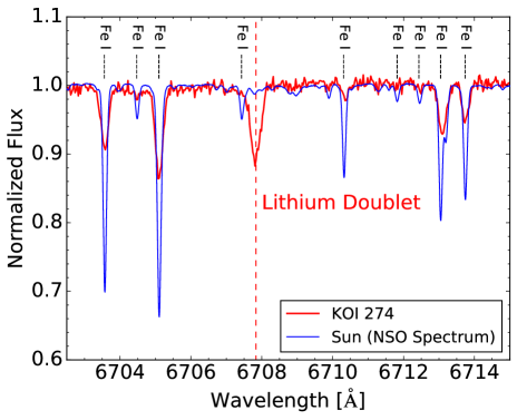
Figure 2: Post-continuum normalization and wavlength calibration spectrum. In red is a HIRES spectrum of KOI 274 ($T_{\mathrm{eff}}$ = 6081 K, $\log g$ = 4.09, and [Fe/H] = –0.03), which has been continuum-normalized and wavelength-calibrated. The blue spectrum is the rest-wavelength solar spectrum from the National Solar Observatory’s Solar Flux Atlas. Significant solar lines are labeled accordingly, including the Li doublet feature indicated by the red dashed vertical line.

In Figure 3, we illustrate the structure of spectra of multiple stars around the 6708 Å Li feature for stars with a range of $T_{\mathrm{eff}}$. These particular stars were chosen because of their similar A(Li), [Fe/H], and small $v\sin{i}$. As a function of $T_{\mathrm{eff}}$, stellar lithium features vary significantly in strength. Note how the Fe lines become slightly stronger as $T_{\mathrm{eff}}$ decreases from top to bottom, while the Li feature becomes much stronger as $T_{\mathrm{eff}}$ decreases. This illustrates the strong relationship between the Li EW and $T_{\mathrm{eff}}$. In the hotter stars, more Li is ionized, so the Li I feature weakens.

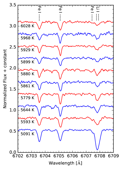
Figure 3: $T_{\mathrm{eff}}$ dependence of the Li doublet. Representative spectra at different $T_{\mathrm{eff}}$ values are plotted here alternating between red and blue lines, all of which have been continuum normalized, wavelength calibrated, and smoothed using a three-point boxcar. These particular spectra were chosen because they have the following ranges in parameter space: 2.12 $\leq$ A(Li) $\leq$ 2.28, -0.04 $\leq$ [Fe/H] $\leq$ 0.16, and $v\sin{i}$ $<$ 6 km/s. We chose these ranges to illustrate how the Fe I lines and Li doublet change with temperature for stars of similar $S/N$, [Fe/H], A(Li), and small $v\sin{i}$.

3.2 Determining the Li EW

Next, we measured the Li EW in the normalized and shifted spectra. The National Institute for Standards and Technology (NIST) has the Li I resonance doublet listed with one transition at 6707.76 and the other at 6707.91 Å. We also had to account for the Fe I line that occurs at 6707.44 Å. Because of the wide variety of spectra at different $T_{\mathrm{eff}}$, [Fe/H], and $v\sin{i}$, it was difficult to find an automated EW measurement routine that was effective for all spectra in our sample.

After testing multiple automated fitting routines/packages, we concluded that Levenberg-Marquardt FIT (LMFIT) (Newville et al. 2014) works well for our purposes; namely, LMFIT can simultaneously fit the Fe line and both Li lines while also providing bounds on each of the fit parameters, unlike other oversimplified methods such as numerical integration or singular Gaussian fits. LMFIT is a non-linear least-square minimization and curve fitting package for Python, which allows users to specify their own composite functions, bounds on parameters, and more. We used a four component composite model. This four component model consisted of a constant = 1 continuum level, one Gaussian for the Fe I line at 6707.44 Å, one Gaussian for the Li I line at 6707.76 Å, and one Gaussian for the Li I line at 6707.91 Å.

In our model, we did not allow the continuum level to vary; we operated under the assumption our continuum normalization requires no adjustment near the Li feature. This assumption is sufficient because the vast majority of CKS stars have $v\sin{i}$ $<$ 15 km/s, in addition to all having $T_{\mathrm{eff}}$ $>$ 4500 K. Therefore, we do not expect significant blending of lines due to the stars’ small $v\sin{i}$, nor significant spectral veiling from the molecular/metal absorption lines of M-dwarfs near the Li doublet. For each of the Gaussians, we implemented similar bounds on the three fitting parameters. We limited their amplitudes to [–1.0, 0.0] to prevent any positive noise fits. We limited the Gaussian widths ($\sigma$) to [0.05, 0.10] to prevent any unphysical, noise-dominated fits. Also, we bounded the set of Gaussian centers to the Fe I line center at 6707.44 Å with physically required separations of 0.32 and 0.47 Å for the Li I 6707.76 and 6707.91 Å lines, respectively, while allowing the group as a whole to shift $\pm$ 0.06 Å. This gives LMFIT the flexibility to shift to fit noisy line profiles but not by more than a resolution element ($\sim$0.12 Å). Unlike other routines, LMFIT sufficiently fits Li absorption features with varying peaks and widths due to the wide range of stellar properties ($T_{\mathrm{eff}}$, $\log g$, $v\sin{i}$, etc.) within the 1305 spectra.

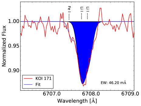
Figure 4: Equivalent width determination for KOI 171 with $S/N=42$. The red curve represents the HIRES spectrum which has been continuum normalized, Doppler-shifted, and smoothed by a three-point boxcar. The blue curve is the best fit from LMFIT’s least-squares minimization process with our composite model. The blue-filled area denotes the integrated EW of the Li I doublet; the calculated EW is shown. Additionally, we indicate the locations of the Li and Fe lines.

Next, we computed the Li EW. See Figure 4 for an illustration of this method. The trough of the Fe line is not centered with respect to the Fe label. This is because the fit was improved by shifting slightly to the right. We emphasize that the calculated EWs do not include contributions from the Fe I line, as illustrated by the blue-filled area in Figure 4. In weak to moderate Li features like those in Figure 4, the feature has a slight asymmetry, caused by a difference in intensity between the smaller wavelength (greater intensity) and larger wavelength (lesser intensity) lines. This can be seen easily with very high resolution and sufficiently high $S/N$ spectra as discussed in Reddy et al. (2002). In our fit, a slight asymmetry is present in the skewed Gaussian from the sum of the blended Li lines.

We defined the uncertainty in our EW measurement, $\sigma_{\mathrm{EW}}$, as the quadratic sum of the $S/N$-per-pixel-dependent Equation (7) ($\sigma_{\mathrm{UL}}$) in Cayrel (1988), and the average of the difference of measured EWs when modifying the continuum level $\pm$ $\frac{1}{S/N_{\mathrm{res}}}$ where $S/N_{\mathrm{res}}$ is the signal-to-noise per resolution element (Bertran de Lis et al. 2015). Due to the limitations of our abundance-determination software, we report and flag our EW measurements according to the following criteria (all reported uncertainties are $\sigma_{\mathrm{EW}}$): if the measured EW $>$ $\sigma_{\mathrm{UL}}+\sigma_{\mathrm{EW}}$, we flag the point as a Li detection and report the measured EW; if $\sigma_{\mathrm{UL}}$ $<$ EW $<$ $\sigma_{\mathrm{UL}}+\sigma_{\mathrm{EW}}$, we report the measured EW but flag the point as an upper limit; if the measured EW $<$ $\sigma_{\mathrm{UL}}$, we report EW = $\sigma_{\mathrm{UL}}$ and flag the point as an upper limit. See Table 1 for the entire sample’s reported EWs.

In Figure 5, we plot the measured EW of all CKS stars as a function of $T_{\mathrm{eff}}$. The upper limits (grey downward arrows) are stars with measured Li EW $<$ $\sigma_{\mathrm{UL}}+\sigma_{\mathrm{EW}}$. From this plot, we can identify young stars: those with large EWs at low $T_{\mathrm{eff}}$. Any $Kepler$ planet host stars with EWs located far above the “slipper” are particularly young. At higher $T_{\mathrm{eff}}$, the slipper is less well-defined largely because we do not have as many of these larger stars, and those that we do have are close to the Li “dip” observed in the Hyades as discussed in Boesgaard et al. (2016).

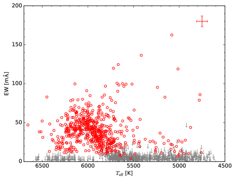
Figure 5: Li EW as a function of effective temperature for all CKS stars. The red points represent stars with Li detections, while the grey downward arrows are Li EW upper limits (EW $<$ $\sigma_{\mathrm{UL}}+\sigma_{\mathrm{EW}}$). Typical error bars are supplied in the upper right corner of the plot for reference.

3.3 Model Atmosphere Interpolation

We utilized Model Atmosphere in Radiative and Convective Scheme (MARCS) (Gustafsson et al. 2008) model atmospheres to convert EW to A(Li). Unlike Kurucz model grids, MARCS grids include the microturbulence parameter ($\xi$) in addition to $T_{\mathrm{eff}}$, $\log g$, and [Fe/H]. In particular, we chose MARCS plane-parallel grids because our sample is primarily composed of main sequence dwarfs. We adopted the microturbulent description of Equations (1) and (2) in Takeda et al. (2013). We then interpolated from the discrete MARCS grids to the model atmospheres representing the adopted CKS stellar parameters.

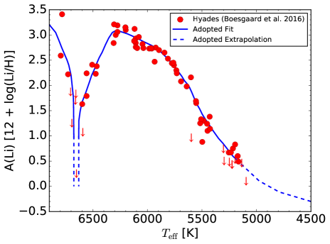
Figure 6: Empirical A(Li) versus $T_{\mathrm{eff}}$ curve for the Hyades. The red points are Hyades data from Boesgaard et al. (2016), where the downward arrows signify upper limits. The blue curve is the approximate fit to this data. The dashed portions of the curve represent regions either where we extrapolated ($T_{\mathrm{eff}}$ $<$ 5100 K) or where we have only upper limits ($T_{\mathrm{eff}}$ $\sim$6650 K).

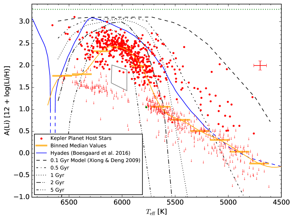
Figure 7: A(Li) as a function of $T_{\mathrm{eff}}$ for 1025 high $S/N$ ($>$ 30) $Kepler$ planet host stars (in red). Downward arrows represent upper limits, while circles are spectra with $EW_{\mathrm{Li}}$ $>$ $\sigma_{\mathrm{UL}}+\sigma_{\mathrm{EW}}$. The orange horizontal bars show the binned median abundances for each of the temperature bins that are 184 K wide and include the upper limits. The orange curve is a cubic spline interpolation between the binned median abundances. The blue curve represents an approximate fit of the Hyades from Boesgaard et al. (2016); the dashed blue line at $T_{\mathrm{eff}}$ $\approx$ 6600 K illustrates the Li “dip” where only upper limits have been measured, while the dashed blue line at $T_{\mathrm{eff}}$ $<$ 5100 K is our adopted extrapolation. The dashed/dotted black lines are from Xiong & Deng (2009) and represent theoretical model isochrones for Li depletion in MS stars. The solid grey polygon at $T_{\mathrm{eff}}$ $\approx$ 6000 K and A(Li) $\approx$ 1.8 is the Li desert illustrated in Ramírez et al. (2012). We plot the meteoric A(Li) = 3.28 $\pm$ 0.05 (Lodders et al. 2009) and photospheric A(Li) = 1.05 $\pm$ 0.10 (Asplund et al. 2009) as the green dotted line and circle, respectively. The red error bars show the sample’s median errors in A(Li) and $T_{\mathrm{eff}}$. Because A(Li) depends sensitively on $T_{\mathrm{eff}}$, we stress that the errors are correlated.

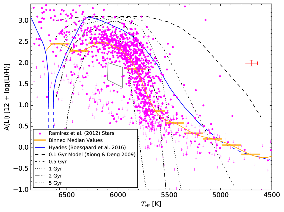
Figure 8: A(Li) as a function of $T_{\mathrm{eff}}$ for 1381 main sequence dwarfs and subgiant stars from Ramírez et al. (2012). We provide this plot as a comparison to the CKS sample. Additionally, we have condensed the natural axes in both $T_{\mathrm{eff}}$ and A(Li) to match Figure 7. As a result, there are $\sim$20 data points outside the range of the chosen axes. Downward arrows represent upper limits, while circles are spectra with measured Li EWs. The orange horizontal bars show the binned median abundances for each of the temperature bins that are 184 K wide as for our sample in Figure 7. The orange fit is a cubic spline interpolation between the binned median abundances. The blue curve represents an approximate fit of the Hyades from Boesgaard et al. (2016); the dashed blue line illustrates the Li “dip” at $T_{\mathrm{eff}}$ = 6600 K where only upper limits have been measured, while the dashed blue line at $T_{\mathrm{eff}}$ $<$ 5100 K is our adopted extrapolation. The dashed/dotted black lines are from Xiong & Deng (2009) and represent theoretical model isochrones for Li depletion in MS stars. The solid grey polygon at $T_{\mathrm{eff}}$ $\approx$ 6000 K and A(Li) $\approx$ 1.8 is the Li desert illustrated in Ramírez et al. (2012). The red error bars show the sample’s median errors in A(Li) and $T_{\mathrm{eff}}$.

3.4 Computing the Lithium Abundance

We determined A(Li) using MOOG (Sneden et al. 2012). This code performs a variety of LTE analysis and spectrum synthesis tasks. We used its $blends$ routine, which computes A(Li). $Blends$ fits abundances of species by using a given model atmosphere to match blended-line EWs. We utilized ${}^{7}\mathrm{Li}$ hyperfine splitting transition wavelengths (Sansonetti et al. 1995) and $gf$ values (Yan & Drake 1995) from Table (3), adapted from Andersen et al. (1984), in Smith et al. (1998) as our line list. We did not include the nearby Fe I line within our line list because we only computed the Li feature’s EW using LMFIT. We then applied $blends$ to determine A(Li) using this line list, in addition to the Li EW and interpolated model atmosphere from §3.2 and §3.3, respectively.

We calculated the uncertainty, $\sigma_{\mathrm{A(Li)}}$, using a similar method to Ramírez et al. (2012). First, we varied each of the MOOG input parameters individually ($T_{\mathrm{eff}}$, $\log g$, [Fe/H], and $EW_{\mathrm{Li}}$) according to their internal CKS 1$\sigma$ errors and then recalculated A(Li). This resulted in two Li abundances, one corresponding to the stellar model after a 1$\sigma$ increase in the varied stellar parameter, A(Li)₊, and the other corresponding to the stellar model after a 1$\sigma$ decrease in the varied stellar parameter, A(Li)_-. Next, we calculated the largest deviation of the upper and lower bound A(Li) values from the A(Li) corresponding to the adopted parameter. We repeated this process for the rest of the MOOG input parameters, and then added the largest deviations of each input parameter in quadrature to determine $\sigma_{\mathrm{A(Li)}}$.

As Bertran de Lis et al. (2015) discussed in their Appendix, adding separate errors in quadrature is insufficient because of the nonlinear transformation between stellar parameters/equivalent widths and abundances. Therefore, our reported A(Li) errors are quantitatively incorrect. However, because we use the largest deviations from A(Li) as our adopted individual uncertainties and then add them in quadrature, we posit that we overestimate the true abundance errors on one side due to the asymmetric distribution of abundances. To appropriately determine each $\sigma_{\mathrm{A(Li)}}$, we would need to perform a Markov Chain Monte Carlo (MCMC) error analysis, which would require an extreme amount of computing time (MOOG would need to be run $>$ 1000 times per star) for the 1305 stars in our sample. In reality, the errors in the individual A(Li) are not particularly important for the results of this paper. Consequently, we conservatively estimate $\sigma_{\mathrm{A(Li)}}$ in the symmetric manner described above.

To ensure the accuracy and precision of MOOG’s $blends$ routine, we compared our EW-A(Li) results to spectral synthesis A(Li) using the same stellar parameters and the Li-blend EW for a subset of 18 stars. We found the measurements to be consistent within 4$\%$.

4 Lithium Abundances

In Figure 6, we plot the empirical A(Li) versus $T_{\mathrm{eff}}$ curve for the Hyades based on data from Boesgaard et al. (2016). We ignored all upper limits while constructing this curve. To construct the Hyades curve, we performed manual linear interpolation of A(Li) as a function of $T_{\mathrm{eff}}$, dictated by the location of individual Hyades stars in this plot. The dashed portions of the curve indicate two separate extrapolations: a) at $T_{\mathrm{eff}}$ $<$ 5100 K, following the smooth curve of the interpolation at higher $T_{\mathrm{eff}}$ and flattening to the upper limits of the CKS sample towards $T_{\mathrm{eff}}$ = 4500 K, and b) at $T_{\mathrm{eff}}$ $\approx$ 6650 K, where only upper limits exist, hence the vertical dropoff. At $T_{\mathrm{eff}}$ $>$ 6800 K, the curve is influenced heavily by a few data points outside the range of this plot.

The blue Hyades curve is important when viewing Figure 7, as it provides an empirical relationship between A(Li), $T_{\mathrm{eff}}$, and age, much like the theoretical isochrones (black, dashed and dotted curves) from Xiong & Deng (2009) do. In Figure 7, the red circles and downward arrows represent detected and upper limit A(Li) values, respectively, for all 1025 CKS $Kepler$ planet host stars that have $S/N$ $>$ 30 spectra. We emphasize that the $T_{\mathrm{eff}}$ and A(Li) errors are correlated, so when we change $T_{\mathrm{eff}}$, A(Li) will be affected as well.

Table 1 contains our entire catalog of A(Li) measurements, including each observation code, KOI number, $S/N$, adopted $T_{\mathrm{eff}}$, adopted $\log g$, adopted [Fe/H], the calculated $\xi$, the measured EW and its uncertainty, and the computed $\sigma_{\mathrm{A(Li)}}$. The entire table, in machine-readable format, can be found in the online version of this journal.

4.1 Identification of Young Stars

Unfortunately, deriving precise ages from measurements of $EW_{\mathrm{Li}}$ and subsequent computation of A(Li) is quite difficult due to the inability of current models (Xiong & Deng 2009) to fit observed abundances. In Figure 7, the distribution of $Kepler$ planet host stars resembles that of the Hyades much better than these Li depletion model isochrones. The orange bars represent the binned median A(Li) for stars with $T_{\mathrm{eff}}$ spanning the width of the bar. The orange curve is a cubic spline interpolation of the orange median A(Li) bars and serves as a statistical representation of the median A(Li) stars at each effective temperature. These stars may represent an empirical isochrone, much like the Hyades do. This curve appears similar in shape to the Hyades curve, while it intersects multiple theoretical model isochrones from Xiong & Deng (2009). Because the theoretical models are unable to match both the Hyades and the distribution of $Kepler$ planet host stars, the ages indicated by each of the black curves prove unreliable. Although numerical ages are difficult to determine, we can use A(Li) versus $T_{\mathrm{eff}}$ plots to distinguish between young (i.e. $<$ 650 Myr) and old systems.

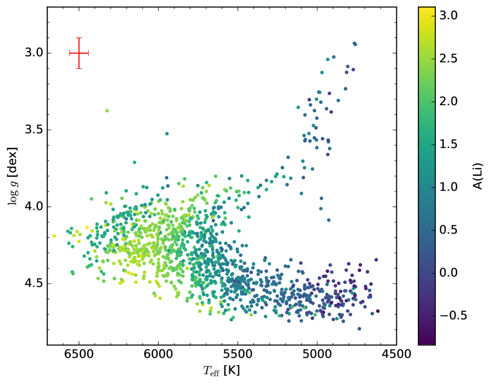
Figure 9: Hertzprung-Russell diagram of $\log g$ as a function of $T_{\mathrm{eff}}$ for all 1305 $Kepler$ planet host stars. The red error bars show the sample’s median errors in $\log g$ and $T_{\mathrm{eff}}$. The color of the points represents A(Li) on a linear scale as illustrated by the color bar on the right.

Stars deplete their surface Li over time. However, the rate of depletion varies with $T_{\mathrm{eff}}$. Cooler stars (K type and later) deplete their Li faster because their convective zone depths are larger than hotter (G-type and earlier) stars. Therefore, we expect to see more stars with high A(Li) at higher $T_{\mathrm{eff}}$, as demonstrated in Figure 7. Naturally, we see a higher proportion of upper limits at cool temperatures compared to hot temperatures. We expect younger stars to have higher A(Li) than other stars at their $T_{\mathrm{eff}}$. With this in mind, we can pick out the youngest stars as those most significantly above the blue Hyades curve and our orange empirical median curve.

Additionally, we can define a sample of stars that are younger than the Hyades by computing:

$$\Delta_{\mathrm{A(Li),Hyades}}=\mathrm{A(Li)}-\mathrm{A(Li)_{Hyades}}$$ (1)

for each star in the sample, where A(Li) is the computed value from the pipeline and A(Li)_Hyades is the interpolated value of the Hyades at the star’s $T_{\mathrm{eff}}$. Stars that are younger than the Hyades will have $\Delta_{\mathrm{A(Li),Hyades}}$ $>$ 0. Table 2 includes all young CKS stars with detected Li (no upper limits are included in the table). The subtraction of the empirical Hyades curve is useful because it removes the offset caused by the $T_{\mathrm{eff}}$ dependence of A(Li).

Figure 7 indicates that stars with A(Li) $>$ 1.0 and $T_{\mathrm{eff}}$ $<$ 5300 K are the youngest systems due to their unusually high A(Li). For comparison, the Hyades is 650 Myr according to estimates from Perryman et al. (1998) and Brandt & Huang (2015). Therefore, stars above the blue Hyades curve should be younger than 650 Myr. In essence, we can determine the relative ages of systems in Figure 7 by subtracting the blue Hyades curve from the $Kepler$ planet host star data points. These A(Li)-$T_{\mathrm{eff}}$ plots also allow the qualitative comparison of average system properties above and below the Hyades.

For a comparison to our CKS sample, we include Figure 8, which contains data from Ramírez et al. (2012). We plot the same structures as those in Figure 7. In Ramírez et al. (2012), the Li desert (outlined as a grey trapezoid in Figures 7 and 8) was emphasized as an area without stars. The authors argued that the Li desert is a physical phenomenon caused by short-lived processes on the stellar surface that deplete Li for 1.1–1.3 $M_{\odot}$ stars. These processes are not well understood, but the observational evidence is hard to ignore. However, our sample produces two stars within this desert. If the Li desert is indeed a physical gap, we conclude that errors in both A(Li) and $T_{\mathrm{eff}}$ can account for this discrepancy. Moreover, Figure 7 (our sample) has a large number of upper limits when compared to Figure 8 (Ramírez et al. 2012). This is due to our low median $S/N\approx 45$ compared to the median $S/N\gtrapprox 100$ from Ramírez et al. (2012). Figure 7 has more cool stars than Figure 8, while Figure 8 has more hot stars. This is an important distinction between the two samples. Faint stars in the CKS sample were chosen because of higher planet multiplicity and/or the presence of interesting planets. Because of this, we have a larger fraction of low $T_{\mathrm{eff}}$ stars compared to Ramírez et al. (2012). Curiously, only one star appears above the Hyades at $T_{\mathrm{eff}}$ $\approx$ 5900–6300 K in Figure 7, while Figure 8 has $\gtrsim$ 10 stars in the same area. Based on the simple assumption of a uniform distribution of stellar ages, Figure 7 should have a few stars above the Hyades at these $T_{\mathrm{eff}}$. This observation puzzles us.

We are also puzzled by the large number of stars within the Li dip in Figure 8. According to the Li depletion mechanisms discussed in Xiong & Deng (2009), the Li dip is a result of gravitational settling of Li into progressively hotter radiative zones in the stellar interior, where it is burned in ($p$,$\alpha$) reactions. Why so many stars from Ramírez et al. (2012) reside in the dip perplexes us. We do not see the same within the CKS sample, but we do not have many stars in that range of $T_{\mathrm{eff}}$.

Table 3 displays the full list of the CKS planets with significant Li detections that are younger than the Hyades. However, we do not incorporate stars with upper limits because their A(Li) are unreliable, nor do we include false positive planet detections in this table.

4.2 Stellar Properties and Age

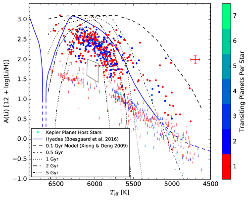
Figure 10: A(Li) as a function of $T_{\mathrm{eff}}$ for 918 $Kepler$ planet host stars. The data in this figure is similar to Figure 7, except all single star planet false positives have been removed. Downward arrows represent upper limits, while circles are stars with $EW_{\mathrm{Li}}$ $>$ $\sigma_{\mathrm{UL}}+\sigma_{\mathrm{EW}}$. The color of the points represents the number of discovered transiting planets in each $Kepler$ system as shown by the discrete color bar on the right.

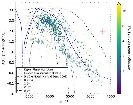
Figure 11: Same as Figure 10, except colors now represent the average planet radius for each system on a continuous, logarithmic scale as shown by the color bar.

We begin our age investigation by analyzing trends in stellar properties with A(Li). We again utilize the A(Li) versus $T_{\mathrm{eff}}$ plot much like Figures 7 and 8, but color the points according to the stellar property of interest. First, we investigate [Fe/H]. We find no significant trends in metallicity with age after comparing stars with A(Li) above and below the Hyades, although a clump of low metallicity points occurs both above and immediately to the right of the Li desert. We arrive at similar conclusions for $\log g$  although there do appear to be some “young” subgiants/giants around $T_{\mathrm{eff}}$ = 5000 K and A(Li) = 1.0. This will become important for clean sample selection later. In addition, the stars with the highest A(Li) at their respective $T_{\mathrm{eff}}$ have high $\log g$.

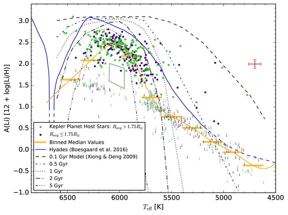
Figure 12: Same axes and labels as Figure 11. From the data in Figure 11, we removed all planets with high impact parameters, those orbiting subgiant and giant stars, and those with low transit signal-to-noise ratios ($S/N$ $<$ 10). Points are colored according to whether the average radius of the planets orbiting that host star is greater than (green) or less than (purple) 1.75$R_{\oplus}$. There are 363 green points and 371 purple points.

Figure 9 is a proxy for a Hertzprung-Russell (HR) Diagram with $\log g$ versus $T_{\mathrm{eff}}$ and points colored by their A(Li). The youngest systems are the brightest (green and yellow colored) points on the main sequence at their respective $T_{\mathrm{eff}}$ and $\log g$. Most stars in the sample are main sequence dwarfs, although the sample also includes the horizontal branch of subgiants and then giants at the top of the “tail” at the lowest $T_{\mathrm{eff}}$ and $\log g$. In addition, this plot reveals A(Li)’s temperature dependence, visible in the smooth transition of colors from hotter to cooler effective temperatures. We note that a few stars on the lower envelope of the main sequence in the figure (at the highest $\log g$) typically have larger A(Li) compared to stars at the same $T_{\mathrm{eff}}$ and slightly lower $\log g$. Current stellar evolution models predict that, as stars evolve during their main sequence lifetimes, they gradually increase in luminosity and inflate in size. Therefore, the stars with the highest $\log g$ values at their respective $T_{\mathrm{eff}}$ are likely some of the youngest stars in our sample.

4.3 Finding and Comparing Exoplanet Properties

Just as we investigated stellar parameters versus age in the previous section, we can apply the same analysis to exoplanet parameters. We use the catalog of exoplanet parameters provided by Johnson et al. (2017) and the NASA Exoplanet Archive to obtain exoplanet parameters for our systems. We note that many of the NASA Exoplanet Archive planet parameters derive from the detailed stellar analysis of Huber et al. (2014). First, we investigate whether planet multiplicity (number of planets discovered per star) varies with age. In Figure 10, single planet systems are colored red, while multi-planet systems range from blue (2 planets) through bright green (7 planets). We compare points above and below the Hyades, and we find no evidence for multiplicity’s dependence on age. Similarly, we investigated whether there are any trends in planet disposition, average planet period, and average planet insolation flux using more A(Li) versus $T_{\mathrm{eff}}$ plots, but no patterns were apparent. Therefore, we conclude that these exoplanetary properties show no dependence on age.

Finally, we consider the average planet radius in each system. A quick look at Figure 11 does not reveal any clear trends between planet radius and location above/below the Hyades. However, many of the identified young systems in §4.1 (those at $T_{\mathrm{eff}}$ $<$ 5500 K and above the Hyades curve) are green and yellow-colored. Therefore, they have large average planet radii. We find this evidence interesting, as planets are expected to deflate as they age and their star remains on the main sequence (Lopez et al. 2012). We continue with a more thorough investigation.

4.4 Planet Radius and Age

Before we proceed, we must consider sample biases and eliminate any systems which may introduce biases in age and planet size. Therefore, we utilize similar cuts to produce a clean sample as in Fulton et al. (2017). First, we eliminate all false positives identified in the CKS (Petigura et al. 2017) and stars with spectral $S/N$ $<$ 30. Next, we remove all planets with impact parameter, $b$, $>$ 0.7 and those orbiting subgiant and giant stars according to Equation (1) in Fulton et al. (2017). Additionally, we remove all planets with low transit signal-to-noise ratios ($S/N$ $<$ 10). These cuts ensure that the planetary radii are reliable and that the host stars are main sequence dwarfs (where A(Li) is a reliable indicator of age). We do not remove planets with long orbital periods and large KepMags because these cuts further reduce our sample’s size, while the likelihood of systematic biases in age and planetary radii of these systems is small.

To make any obscured trends more apparent in Figure 11, we split the sample into two parts: systems with $R_{\mathrm{avg}}>1.75R_{\oplus}$ and those with $R_{\mathrm{avg}}\leq 1.75R_{\oplus}$. We choose 1.75$R_{\oplus}$ as our separating radius because it corresponds to the trough of the empirical gap revealed in Fulton et al. (2017). Figure 12 displays our “clean” sample in another A(Li)–$T_{\mathrm{eff}}$ comparison plot with the points colored according to their average planet radius.

We observe from Figure 12 that the stars younger than the Hyades typically have planet companions on the large side of the planet radius gap discovered by Fulton et al. (2017). The prevalence of green points above the Hyades supports the conclusion that younger planets are larger than older planets. However, because this plot assigns an average planet radius to each star, we lose information about individual planetary radii. Therefore, we must perform additional statistical analysis to test our hypothesis that, on average, larger planets orbit younger stars.

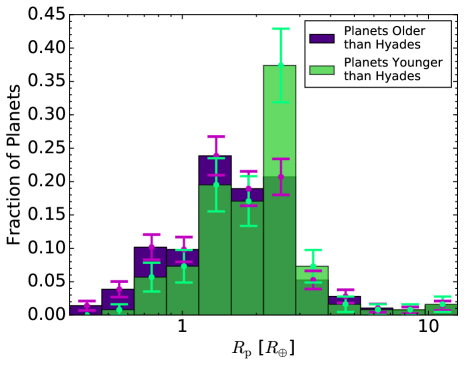
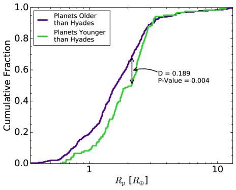
Figure 13: Planet radius distributions for planets older (purple) and younger (green) than the Hyades, while all planets meet the following criteria: host spectral $S/N$ $>$ 10, host $T_{\mathrm{eff}}$ $<$ 5500 K, host is on the main sequence, planet is not a false positive, planet impact parameter $b$ $<$ 0.7, and planet transit $S/N$ $>$ 10. $Top$: Normalized histograms for $R_{\mathrm{p}}$. We include Poisson error bars on each of the bins for reference. $Bottom$: Cumulative fraction of planets as a function of $R_{\mathrm{p}}$. We have labeled the K-S statistic, which represents the greatest distance between the two distributions, as D. The largest difference occurs at $R_{\mathrm{p}}\simeq 2.0R_{\oplus}$. The labeled p-value indicates that, at $\sim$3$\sigma$ significance, we can reject the null hypothesis that the two samples come from the same parent distribution.

4.5 A Statistical Comparison of Old and Young Systems

To differentiate between young and old systems, we use the Hyades as the dividing line. The Hyades is $\sim$650 Myr old (Perryman et al. 1998; Brandt & Huang 2015; Boesgaard et al. 2016); systems that fall above (below) it in A(Li) versus $T_{\mathrm{eff}}$ space (see Figure 12) are younger (older) than the Hyades. This statement holds true for the majority of systems, but those close to the Hyades curve are more likely to be on the wrong side of the Hyades curve. Errors in measurement and potential abundance effects ($i.e.$ differences in initial A(Li)) affect our young/old system designation in detail. We do not expect the measurement errors to systematically bias our results. In addition, while abundance effects may introduce a systematic bias ($i.e.$ Kepler stars have systematically higher initial A(Li) compared to the Hyades), ensembles of stars have been shown to give consistent initial A(Li) although the individual scatter may be large (Soderblom 2010). Much like the measurement errors are unlikely to introduce systematic bias, scatter in the initial A(Li) for our Kepler stars should not introduce systematic effects in our reported A(Li). We note that the Hyades’s curve does not extend far enough at low $T_{\mathrm{eff}}$ for us to compare systems with stellar $T_{\mathrm{eff}}$ $\lesssim 5100$ K. Therefore, we extrapolate the Hyades curve to low $T_{\mathrm{eff}}$ to solve this issue. We choose the observed median curve from the CKS sample as our adopted extrapolation (blue dashed line at low $T_{\mathrm{eff}}$ in A(Li)–$T_{\mathrm{eff}}$ plots) because it appears to follow the A(Li)-$T_{\mathrm{eff}}$ relationship of the Hyades at low $T_{\mathrm{eff}}$.

Before we begin any detailed statistical tests, we must again eliminate any systems which may introduce bias. We removed all planets/systems discussed at the beginning of §4.4, in addition to systems with $T_{\mathrm{eff}}$ $>$ 5500 K because our sample of young systems at higher $T_{\mathrm{eff}}$ is incomplete. However, we do re-include stars with spectral $S/N$ = 10–30 because some of these systems include significant Li detections. We also note that ignoring these stars significantly reduces the size of our available sample. After making these cuts, 257 systems that host 408 exoplanet candidates remained.

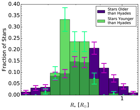
Figure 14: Stellar radius normalized histograms for stars older (purple) and younger (green) than the Hyades, while all stars meet the following criteria: spectral $S/N$ $>$ 10, $T_{\mathrm{eff}}$ $<$ 5500 K, star is on the main sequence, hosted planet is not a false positive, hosted planet impact parameter $b$ $<$ 0.7, and hosted planet transit $S/N$ $>$ 10. We include Poisson error bars on each of the bins for reference.

We separated the two groups into old ($\Delta_{\mathrm{A(Li),Hyades}}\leq 0$) and young ($\Delta_{\mathrm{A(Li),Hyades}}>0$) systems. We placed these points into $R_{\mathrm{p}}$ bins and plotted the resulting normalized histograms (see top plot of Figure 13). There are 285 old planets (purple histogram) and 123 young planets (green histogram). We also performed a two-sided/two-sample K-S test to determine if the two distributions are from different parent populations. We plot the cumulative fraction of planets in $R_{\mathrm{p}}$ and the K-S test result in the bottom panel of Figure 13. With a p-value of 0.004, we reject the hypothesis that the two samples were drawn from the same parent distribution at a statistical significance of $\sim$3$\sigma$. Therefore, we conclude that old and young systems represent distinct populations in $R_{\mathrm{p}}$ space. The median value for the young planets is $R_{\mathrm{p}}$ = 2.13 $\pm$ 0.01 $R_{\oplus}$, while the median value for the old planets is $R_{\mathrm{p}}$ = 1.61 $\pm$ 0.01 $R_{\oplus}$.

To ensure we are not being fooled by potential confounding factors (such as transit $S/N$ limitations of small planets around larger stars), we plot the stellar radius distributions (Petigura et al. 2017) of stars younger (green) and older (purple) than the Hyades in Figure 14 as we do planets in Figure 13. From Figure 14, we observe that the stars younger than the Hyades are systematically smaller than their older counterparts. This limits the possibilities for artificial inflation of younger planets. We note that the stars are primarily in the range of 0.6–1.0 $R_{\mathrm{\odot}}$. From transit $S/N$ considerations and these stellar radius distributions, it is likely that we can detect smaller planets around the younger stars if they were present. Ultimately, we conclude that our young stars are smaller and unlikely to explain the difference we see in the old and young planet radii distributions.

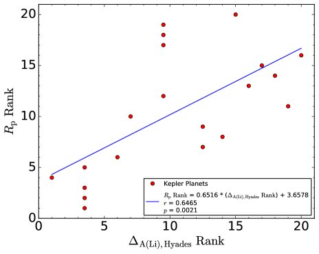
Figure 15: Spearman rank-order correlation coefficient test for $R_{\mathrm{p}}$ and $\Delta_{\mathrm{A(Li),Hyades}}$. We have removed all subgiant and giant stars, stars with $T_{\mathrm{eff}}$ $>$ 5500 K, stars with upper limit A(Li), stars with $\Delta_{\mathrm{A(Li),Hyades}}<0$ (old stars), false positive planets, planets with $b>0.7$, and planets with transit $S/N$ $<$ 10. The red points are the rank-orders of the remaining Kepler planets in $R_{\mathrm{p}}$ and $\Delta_{\mathrm{A(Li),Hyades}}$, while the blue line is the line of best fit. The legend includes the equation for the line of best fit, as well as $r$, the correlation coefficient, and $p$, the likelihood that our two parameters are uncorrelated.

As has been demonstrated by Babu & Feigelson (2006), the one sample K-S test and other empirical distribution functions can be unreliable when using them to determine the parameters of best-fit models. Fortunately, we are using a two sample K-S test to compare two populations within our data – not using it to determine parameters of those populations. Despite the utility of the two sample K-S statistic, according to Engmann & Cousineau (2011), this statistic is inferior to the two sample Anderson-Darling (A-D) statistic. The A-D test is more proficient in detecting differences in shift, scale, and symmetry between samples from two different distributions. Thus, we perform a two sample A-D test on the same sample used for the two sample K-S test. Our resulting normalized A-D statistic is 5.98, corresponding to a p-value of 0.002 ($>3\sigma$). Unsurprisingly, we report a more significant A-D p-value than K-S p-value.

However, these results are not robust: if we remove systems with $S/N$ $<$ 30 from our sample, our K-S p-value rises to 0.48 and our A-D p-value rises to 0.37, which both correspond to a statistical significance of $<$ 1$\sigma$. This is not sufficiently significant to definitively conclude that exoplanet radii decrease as exoplanets age. Removing these moderate-$S/N$ ($10<S/N<30$) systems reduces the number of old planets from 285 to 212 and the number of young planets from 123 to 43. We argue that including moderate-$S/N$ systems is important for the K-S and A-D tests because without them we are left with a very small sample of younger planets, insufficient for statistical distribution comparisons with the older planets.

We also perform additional statistical analyses, including Pearson and Spearman rank-order correlation coefficient tests of the relation between $R_{\mathrm{p}}$ and $\Delta_{\mathrm{A(Li),Hyades}}$. We use these tests to analyze 20 exoplanet candidates that remain after removing all of the following stars and planets: subgiants and giants, $T_{\mathrm{eff}}$ $>$ 5500 K, upper limit A(Li), stars with $\Delta_{\mathrm{A(Li),Hyades}}<0$ (old stars), stars with spectral $S/N$ $<$ 10, false positive planets, planets with $b>0.7$, and planets with transit $S/N$ $<$ 10. We remove all upper limits in A(Li) because ages of these systems are inherently uncertain. In addition, we eliminate old stars and planets because these systems/planets contaminate the theoretically predicted relationship between planet size and age in younger systems (Lopez et al. 2012). The Spearman rank-order test is more reliable than the Pearson test because it assumes nothing about the underlying relationship between planet radius and age, unlike the Pearson test which assumes a linear relationship.

We plot the results of the Spearman test in Figure 15, and we report that the Spearman test returns a positive correlation between planet radius and A(Li) relative to the Hyades. The figure has a strong, positive correlation coefficient ($r$ = 0.6465), and a small p-value ($p$ = 0.0021). We performed a similar analysis using the Pearson correlation coefficient test for comparison. Unsurprisingly, the Spearman correlation coefficient is stronger than the Pearson coefficient. Unlike the K-S and A-D test results, these correlation coefficients are robust and not sensitive to changes in parameter ranges. Although the p-value indicates a high significance of correlation between planet radius and the relative age of these systems, our small sample size makes it difficult to trust these p-values at their reported significance. Nevertheless, the combination of the low p-value and the strong, positive correlation coefficient between planet radius and age support the current models of young exoplanet evolution.

5 Discussion

Our findings are suggestive that larger planets are more likely to orbit younger stars. Lopez et al. (2012) discuss a few possible mechanisms, including cooling and atmosphere loss, that cause planets to contract over time. The authors choose typical timescales of 10 Myr and 100 Myr for cooling and contraction after formation. Notably, the youngest stars in our sample fall close to the 100 Myr isochrone from Xiong & Deng (2009), which may indicate that these planets are still inflated from a combination of residual heat from formation and extreme ultraviolet (XUV) flux received from their host star. Interestingly, the planet radius gap discussed in Fulton et al. (2017) separates the calculated median planet radius for older planets ($R_{\mathrm{p}}$ = 1.61 $R_{\oplus}$) from the calculated median planet radius for younger planets ($R_{\mathrm{p}}$ = 2.13 $R_{\oplus}$).

Additionally, Lopez et al. (2012) investigate the $Kepler$-11 system and the possible formation mechanisms for each of the planetary companions. Figure 2 in this paper provides an illustration of the degeneracy in producing the radius of $Kepler$-11b. Its current radius could be just as easily explained by a 0.3% H/He composition or an 11% H/He composition. The authors state that most of the mass (and radius) loss happens in the first Gyr. Our finding of larger planets orbiting younger stars agree with their models.

Heat from formation and XUV radiation are not the only parameters that impact mass (and radius) loss. Lopez & Fortney (2013), in looking at the $Kepler$-36 system, found that core mass plays a large role in the evolution of the radius of a planet. However, $Kepler$ data do not include the masses of most of the CKS planets, so it is difficult for us to conclude anything about their compositions and whether that has an effect on the observed distribution of young systems.

Moreover, Lopez et al. (2012) considered the hydrodynamic mass loss of close-in, low-mass, low-density (LMLD) planets from the XUV radiation released by their young MS stars. Mass loss rates are much larger when planets are young because of (1) planetary radii are considerably larger due to heat from formation and (2) a star’s $F_{\mathrm{XUV}}$ is $\sim$500 times higher at 100 Myr than the same star’s $F_{\mathrm{XUV}}$ at a few Gyrs (Lopez et al. 2012). Fortney et al. (2007) provides a plot of $R_{\mathrm{p}}$ versus age for a few masses ranging from 0.1–3.0 $M_{\mathrm{J}}$ at various orbital radii. Planets closer than 0.045 AU to a solar analog star are significantly affected by the XUV radiation, while those further away are minimally impacted. Therefore, we calculated the corresponding insolation flux at 0.045 AU ($\approx$500 $F_{\oplus}$), and used this criterion to limit our sample of young and old planets. All planets with $F_{\mathrm{p}}>500F_{\oplus}$ were excluded to determine if, statistically, we could separate residual heat from formation inflation from XUV heating inflation. However, we found the old and young planet $R_{\mathrm{p}}$ distributions were more similar than those with no exclusions based on $F_{\mathrm{p}}$.

Because we ignored evolved stars and the number of Jupiter-size planets included in the CKS is small, we were unable to test the planet reinflation theories detailed in Grunblatt et al. (2016). Nevertheless, our results do provide evidence for the shrinking of planets as they orbit their main sequence stars; interestingly, planet shrinkage during their host’s main sequence lifetime is an initial condition for post-main sequence planet reinflation.

We find no evidence for a correlation between between age and other planet parameters, such as $Kepler$ planet multiplicity, orbital period, and insolation flux. This is unsurprising on the large scales we consider in this paper. $Kepler$ planet multiplicity is inherently uncertain given that our planet detections for any star are, by no means, complete. We may expect to see less planets around the older stars due to dynamical interactions (and potential planet ejection) in those systems, but these interactions typically happen very early in the host’s lifetime. We expect the incompleteness of our planet sample to trump any age effects. Orbital periods are extremely precise compared to other planet property determinations, but it is unclear whether there exist any processes to systematically bias old planets’ orbital periods relative to young planets’ orbital periods. The variation in orbital period from system to system likely dominates over proposed processes such as planet migration that can lead to different old and young planet populations. In addition, insolation flux is mostly a function of stellar luminosity ($i.e.$ stellar mass/radius), which, as Figure 14 illustrates, introduces systematic bias between systems older and younger than the Hyades. Thus, any age effects on insolation flux are insignificant compared to the differences in initial conditions.

6 Summary and Conclusions

In this paper, we have detailed our automated Li pipeline from normalization of the spectra to the determination of A(Li). With these data, we produced a catalog of A(Li), which includes the relevant stellar properties and errors. We proceeded to compare stellar properties ($\log g$ and [Fe/H]) with A(Li) through A(Li)-$T_{\mathrm{eff}}$ plots, and found no trends with A(Li). Additionally, we compared exoplanet properties using the same A(Li)-$T_{\mathrm{eff}}$ plots. We found that most exoplanet properties ($Kepler$ planet disposition, multiplicity, orbital period, and insolation flux) do not trend with A(Li). Raw A(Li) values are not the best age differentiator, as A(Li) varies with $T_{\mathrm{eff}}$, so we use our interpolated empirical Hyades curve (Figure 6) derived from Boesgaard et al. (2016) to separate systems older and younger than 650 Myr. Because A(Li) relative to the Hyades is a proxy for the age of FGK main sequence dwarfs, we conclude that these exoplanet properties show no trends with relative age. However, we do find statistical evidence for the shrinking of exoplanet radii with age based on K-S, Pearson, and Spearman tests.

We conclude that the difference in the $R_{\mathrm{p}}$ distributions of young and old systems suggests exoplanet radii shrink as they age during their host’s main sequence lifetime, a phenomenon that may result from a combination of photoevaporation of the planets’ atmospheres and cooling (and contraction) from the planets’ residual heat from formation. We look forward to future surveys that link exoplanet properties and age. These studies may reveal paramount information about the mechanisms of exoplanet formation and evolution, as well as the processes behind our own Solar System’s origin.

Table 1: Pipeline Results for $Kepler$ Planet Host Stars

Obs Code	Obs Date	KOI	KepMag	$S/N$	$T_{\mathrm{eff}}$ [K]	$\log g$ [dex]	[Fe/H]	$\xi$ [km/s]	$EW_{\mathrm{Li}}$ [mÅ]	A(Li) [dex]
j122.742	2011-06-16	1	11.34	39	5819	4.40	0.01	1.04	85.5 $\pm$ 7.9	2.62 $\pm$ 0.08
j122.92	2011-06-13	2	10.46	39	6449	4.13	0.20	1.77	82.9 $\pm$ 7.3	3.11 $\pm$ 0.07
j122.81	2011-06-13	3	9.17	41	4864	4.50	0.33	0.54	4.2 $\pm$ 5.1	$<$ -0.40
j70.1247	2009-06-05	6	12.16	119	6348	4.36	0.04	1.58	15.4 $\pm$ 2.2	2.16 $\pm$ 0.08
j74.509	2009-07-31	7	12.21	126	5827	4.09	0.18	1.17	54.0 $\pm$ 2.1	2.36 $\pm$ 0.06
j70.1251	2009-06-05	8	12.45	89	5891	4.54	-0.07	1.05	54.5 $\pm$ 3.6	2.42 $\pm$ 0.06
j77.875	2009-10-05	10	13.56	74	6181	4.24	-0.08	1.46	19.7 $\pm$ 3.6	2.15 $\pm$ 0.10
j72.483	2009-07-03	17	13.30	77	5660	4.15	0.36	1.09	2.3 $\pm$ 2.3	$<$ 0.75
j72.487	2009-07-03	18	13.37	73	6332	4.12	0.02	1.66	52.3 $\pm$ 3.8	2.75 $\pm$ 0.06
j93.303	2010-06-26	20	13.44	103	5927	4.01	0.03	1.30	40.7 $\pm$ 2.6	2.31 $\pm$ 0.06
j76.1283	2009-09-05	22	13.44	79	5891	4.21	0.21	1.19	25.8 $\pm$ 3.7	2.04 $\pm$ 0.09
j126.89	2011-07-09	41	11.20	207	5854	4.07	0.10	1.21	34.3 $\pm$ 1.3	2.15 $\pm$ 0.06
j90.90	2010-05-01	42	9.36	212	6306	4.28	-0.01	1.57	15.7 $\pm$ 1.3	2.14 $\pm$ 0.06
j124.500	2011-06-23	46	13.77	50	5661	4.07	0.39	1.12	98.2 $\pm$ 5.5	2.57 $\pm$ 0.07
j120.1133	2011-05-26	49	13.70	46	5779	4.34	-0.06	1.10	3.8 $\pm$ 4.6	$<$ 1.07
j130.1072	2011-08-18	63	11.58	181	5673	4.68	0.25	0.94	90.3 $\pm$ 1.6	2.41 $\pm$ 0.06
j76.1081	2009-09-04	64	13.14	92	5357	3.86	0.09	1.01	3.3 $\pm$ 2.9	$<$ 0.62
j76.1276	2009-09-05	69	9.93	163	5594	4.41	-0.09	0.97	1.2 $\pm$ 1.6	$<$ 0.38
j97.1478	2010-08-24	70	12.50	133	5508	4.47	0.11	0.91	3.3 $\pm$ 2.1	$<$ 0.71
$\cdots$	$\cdots$	$\cdots$	$\cdots$	$\cdots$	$\cdots$	$\cdots$	$\cdots$	$\cdots$	$\cdots$	$\cdots$

Note. — Observational and stellar data for the CKS stars analyzed in this paper. The stellar parameters $T_{\mathrm{eff}}$, $\log g$, and [Fe/H] have uncertainties of 60 K, 0.10 dex, and 0.04 dex, respectively; these are the adopted values from Petigura et al. (2017). The KepMag column is from the NASA Exoplanet Archive. The other columns ($S/N$, $\xi$, $EW_{\mathrm{Li}}$, and A(Li)) and their uncertainties, where relevant, were computed by our pipeline. We employ Takeda et al. (2013)’s treatment of $\xi$. All items in the table with $<$ symbols in the final column indicate stars with $EW_{\mathrm{Li}}$ $<$ $\sigma_{\mathrm{UL}}+\sigma_{\mathrm{EW}}$, which we have flagged as upper limits in our analysis (and downward arrows in our plots). The full table, in machine-readable format, can be found online.

Table 2: Stars Younger than the Hyades

KOI	$S/N$	$T_{\mathrm{eff}}$ [K]	$\log g$ [dex]	[Fe/H]	$\xi$ [km/s]	$EW_{\mathrm{Li}}$ [mÅ]	A(Li) [dex]	$\Delta_{\mathrm{A(Li),Hyades}}$ [dex]
1	39	5819	4.40	0.01	1.04	85.5 $\pm$ 7.9	2.62 $\pm$ 0.08	0.08
2	39	6449	4.13	0.20	1.77	82.9 $\pm$ 7.3	3.11 $\pm$ 0.07	0.59
46	50	5661	4.07	0.39	1.12	98.2 $\pm$ 5.5	2.57 $\pm$ 0.07	0.47
63	181	5673	4.68	0.25	0.94	90.3 $\pm$ 1.6	2.41 $\pm$ 0.06	0.27
98	71	6500	4.22	0.05	1.78	52.1 $\pm$ 4.0	2.87 $\pm$ 0.06	0.62
119	47	5681	3.86	0.37	1.19	100.6 $\pm$ 6.4	2.60 $\pm$ 0.07	0.43
149	42	5708	3.95	0.03	1.18	55.3 $\pm$ 7.2	2.27 $\pm$ 0.09	0.02
323	53	5529	4.72	0.10	0.84	52.9 $\pm$ 5.4	1.98 $\pm$ 0.09	0.42
331	42	5506	3.90	0.11	1.08	40.2 $\pm$ 6.8	1.91 $\pm$ 0.11	0.44
660	53	5320	3.89	-0.07	0.98	25.6 $\pm$ 5.4	1.49 $\pm$ 0.13	0.61
684	59	5287	3.84	0.10	0.98	26.3 $\pm$ 5.0	1.47 $\pm$ 0.12	0.67
720	50	5260	4.68	0.04	0.71	14.5 $\pm$ 5.5	1.11 $\pm$ 0.23	0.39
853	28	4876	4.73	-0.02	0.47	43.8 $\pm$ 11.0	1.17 $\pm$ 0.20	1.18
1019	156	5018	3.55	0.17	0.92	7.1 $\pm$ 1.7	0.51 $\pm$ 0.14	0.32
1117	48	6513	4.16	-0.02	1.82	38.3 $\pm$ 6.4	2.72 $\pm$ 0.10	0.53
1175	43	5640	3.80	0.10	1.19	46.8 $\pm$ 7.1	2.12 $\pm$ 0.10	0.08
1199	39	4772	4.53	0.11	0.48	85.9 $\pm$ 8.7	1.28 $\pm$ 0.13	1.40
1208	46	6417	4.16	-0.07	1.73	48.3 $\pm$ 6.1	2.77 $\pm$ 0.08	0.12
1221	106	5002	3.62	0.33	0.89	9.0 $\pm$ 2.4	0.52 $\pm$ 0.16	0.36
1230	51	5119	3.35	0.01	1.04	26.8 $\pm$ 5.4	1.31 $\pm$ 0.13	0.92
1413	34	5253	3.79	-0.03	0.98	18.1 $\pm$ 8.3	1.26 $\pm$ 0.29	0.56
1438	33	5722	3.94	0.19	1.19	64.2 $\pm$ 9.5	2.36 $\pm$ 0.10	0.07
1463	136	6532	4.19	-0.04	1.83	38.2 $\pm$ 2.0	2.73 $\pm$ 0.05	0.66
1800	43	5621	4.69	0.07	0.90	100.1 $\pm$ 6.4	2.49 $\pm$ 0.08	0.51
1839	51	5517	4.67	0.17	0.85	99.4 $\pm$ 5.3	2.28 $\pm$ 0.08	0.77
1864	42	5620	3.93	0.12	1.14	52.1 $\pm$ 7.7	2.15 $\pm$ 0.10	0.18
1985	42	4950	4.64	0.01	0.54	10.3 $\pm$ 5.9	0.62 $\pm$ 0.40	0.55
2033	38	5051	4.53	-0.12	0.64	12.9 $\pm$ 7.5	0.61 $\pm$ 0.40	0.35
2035	48	5558	4.67	0.10	0.87	56.2 $\pm$ 5.5	2.06 $\pm$ 0.09	0.38
2046	45	5579	4.07	0.23	1.07	44.4 $\pm$ 6.4	2.04 $\pm$ 0.10	0.25
2115	13	5239	4.71	0.13	0.68	95.3 $\pm$ 23.1	1.90 $\pm$ 0.20	1.24
2175	42	5459	3.91	0.13	1.06	43.8 $\pm$ 7.1	1.91 $\pm$ 0.11	0.61
2228	41	6656	4.19	-0.10	1.95	47.0 $\pm$ 6.7	2.92 $\pm$ 0.09	4.38
2261	36	5176	4.70	0.06	0.65	31.4 $\pm$ 7.7	1.34 $\pm$ 0.17	0.83
2479	43	5372	3.88	0.08	1.02	28.7 $\pm$ 6.7	1.61 $\pm$ 0.14	0.59
2516	35	5431	3.91	0.30	1.04	19.1 $\pm$ 8.1	1.48 $\pm$ 0.26	0.27
2541	40	5090	3.70	0.15	0.91	15.9 $\pm$ 6.9	0.96 $\pm$ 0.27	0.62
2639	24	5583	3.89	-0.02	1.13	99.4 $\pm$ 13.2	2.50 $\pm$ 0.11	0.69
2640	48	4896	3.02	-0.13	1.01	10.6 $\pm$ 5.6	0.63 $\pm$ 0.34	0.61
2675	45	5756	4.63	0.13	1.00	82.1 $\pm$ 6.2	2.53 $\pm$ 0.07	0.13
2678	43	5416	4.70	0.12	0.78	136.4 $\pm$ 6.4	2.42 $\pm$ 0.09	1.26
2748	44	5499	4.00	-0.06	1.05	33.0 $\pm$ 6.2	1.81 $\pm$ 0.12	0.37
2769	54	5787	3.96	-0.02	1.22	69.4 $\pm$ 5.8	2.47 $\pm$ 0.07	0.00
2831	38	5752	3.92	-0.01	1.21	65.8 $\pm$ 7.1	2.40 $\pm$ 0.09	0.02
2859	46	5260	4.51	-0.07	0.76	12.4 $\pm$ 6.1	0.98 $\pm$ 0.32	0.26
2885	45	5492	3.93	-0.36	1.07	27.5 $\pm$ 6.1	1.70 $\pm$ 0.13	0.29
2891	47	6142	4.02	0.14	1.51	99.8 $\pm$ 5.8	2.99 $\pm$ 0.06	0.01
3012	39	5493	4.16	-0.50	1.00	24.0 $\pm$ 7.3	1.63 $\pm$ 0.18	0.22
3202	41	5262	3.80	0.03	0.98	23.9 $\pm$ 6.7	1.40 $\pm$ 0.17	0.68
3239	47	5668	4.66	0.09	0.94	124.5 $\pm$ 5.7	2.70 $\pm$ 0.07	0.58
3244	58	4970	3.13	-0.03	1.02	25.1 $\pm$ 4.8	1.11 $\pm$ 0.12	1.01
3371	45	5428	4.56	0.00	0.84	54.1 $\pm$ 7.2	1.98 $\pm$ 0.10	0.78
3473	37	5157	4.65	0.05	0.66	82.6 $\pm$ 7.4	1.85 $\pm$ 0.11	1.38
3835	45	5013	4.70	0.04	0.56	118.8 $\pm$ 6.1	1.92 $\pm$ 0.11	1.73
3871	49	5193	4.62	0.07	0.69	11.0 $\pm$ 5.6	0.87 $\pm$ 0.33	0.32
3876	40	5720	4.64	0.12	0.98	119.8 $\pm$ 6.7	2.73 $\pm$ 0.07	0.45
3886	47	4760	2.94	0.20	0.96	11.5 $\pm$ 6.3	0.45 $\pm$ 0.36	0.58
3891	52	5080	3.75	-0.10	0.89	21.6 $\pm$ 5.2	1.08 $\pm$ 0.15	0.76
3908	49	5721	3.88	0.03	1.21	58.1 $\pm$ 6.6	2.30 $\pm$ 0.09	0.02
3936	55	5081	4.66	0.17	0.61	162.5 $\pm$ 4.8	2.03 $\pm$ 0.12	1.71
3991	41	5606	4.62	-0.02	0.92	96.7 $\pm$ 6.6	2.48 $\pm$ 0.08	0.56
4004	52	5739	4.68	-0.05	0.97	78.6 $\pm$ 5.2	2.48 $\pm$ 0.07	0.13
4146	50	5092	4.64	0.24	0.62	22.4 $\pm$ 5.9	0.67 $\pm$ 0.19	0.32
4156	41	5807	4.05	0.24	1.17	96.8 $\pm$ 7.1	2.69 $\pm$ 0.07	0.18
4226	39	5844	3.87	0.35	1.28	82.6 $\pm$ 7.6	2.62 $\pm$ 0.08	0.03
4556	48	5437	3.83	-0.11	1.07	25.5 $\pm$ 6.0	1.61 $\pm$ 0.14	0.39
4613	46	5443	4.55	-0.13	0.85	23.6 $\pm$ 6.7	1.45 $\pm$ 0.17	0.20
4647	31	5166	3.81	0.23	0.92	23.2 $\pm$ 9.6	1.18 $\pm$ 0.25	0.69
4663	52	5545	3.88	0.30	1.11	55.1 $\pm$ 6.6	2.12 $\pm$ 0.09	0.49
4686	47	5698	3.90	0.33	1.19	75.6 $\pm$ 5.9	2.44 $\pm$ 0.07	0.22
4745	14	4781	4.56	0.02	0.47	78.8 $\pm$ 14.6	1.41 $\pm$ 0.16	1.53
4763	36	5695	3.98	0.17	1.17	52.4 $\pm$ 7.8	2.23 $\pm$ 0.10	0.02
4775	43	5210	3.80	0.47	0.95	36.6 $\pm$ 6.3	1.48 $\pm$ 0.11	0.90
4811	31	5572	3.90	0.05	1.12	39.9 $\pm$ 9.4	1.97 $\pm$ 0.15	0.22
4834	50	5030	3.75	0.40	0.86	19.5 $\pm$ 5.4	0.86 $\pm$ 0.16	0.64
5057	38	5004	3.30	0.00	0.99	26.5 $\pm$ 7.1	1.17 $\pm$ 0.16	1.01
5107	27	4933	3.04	-0.13	1.03	27.4 $\pm$ 10.4	1.11 $\pm$ 0.24	1.05
5119	35	4984	3.25	0.08	0.99	13.7 $\pm$ 7.3	0.84 $\pm$ 0.35	0.71
6676	34	6493	4.18	-0.19	1.79	31.1 $\pm$ 8.1	2.59 $\pm$ 0.15	0.31
6759	33	5494	3.90	0.36	1.08	66.2 $\pm$ 8.2	2.16 $\pm$ 0.09	0.75

Note. — CKS stars with Li detections younger than the Hyades. The stellar parameters $T_{\mathrm{eff}}$, $\log g$, and [Fe/H] have uncertainties of 60 K, 0.10 dex, and 0.04 dex, respectively; these are the adopted values from Petigura et al. (2017). The other columns ($S/N$, $\xi$, $EW_{\mathrm{Li}}$, A(Li), and $\Delta_{\mathrm{A(Li),Hyades}}$) and their uncertainties, where relevant, were computed by our pipeline. We employ Takeda et al. (2013)’s treatment of $\xi$. We do not include upper limits in this table.

Table 3: Planets Younger than the Hyades

KOI	$T_{\mathrm{eff}}$ [K]	$EW_{\mathrm{Li}}$ [mÅ]	A(Li) [dex]	$\Delta_{\mathrm{A(Li),Hyades}}$ [dex]	Planet Number	$R_{\mathrm{p}}$ [$R_{\oplus}$]	Period [days]	$F_{\mathrm{p}}$ [$F_{\oplus}$]
1	5819	85.5 $\pm$ 7.9	2.62 $\pm$ 0.08	0.08	1	$14.3^{+1.4}_{-1.4}$	$2.5^{+0.0}_{-0.0}$	$890.7^{+184.9}_{-184.9}$
2	6449	82.9 $\pm$ 7.3	3.11 $\pm$ 0.07	0.59	1	$13.4^{+2.0}_{-2.0}$	$2.2^{+0.0}_{-0.0}$	$3029.6^{+931.2}_{-931.2}$
46	5661	98.2 $\pm$ 5.5	2.57 $\pm$ 0.07	0.47	1	$5.7^{+0.7}_{-0.7}$	$3.5^{+0.0}_{-0.0}$	$1030.6^{+279.4}_{-279.4}$
$\cdots$	$\cdots$	$\cdots$	$\cdots$	$\cdots$	2	$1.2^{+0.2}_{-0.2}$	$6.0^{+0.0}_{-0.0}$	$497.1^{+132.2}_{-132.2}$
63	5673	90.3 $\pm$ 1.6	2.41 $\pm$ 0.06	0.27	1	$6.1^{+0.5}_{-0.5}$	$9.4^{+0.0}_{-0.0}$	$109.0^{+18.3}_{-18.3}$
98	6500	52.1 $\pm$ 4.0	2.87 $\pm$ 0.06	0.62	1	$8.5^{+1.0}_{-1.0}$	$6.8^{+0.0}_{-0.0}$	$572.2^{+142.3}_{-142.3}$
119	5681	100.6 $\pm$ 6.4	2.60 $\pm$ 0.07	0.43	2	$7.2^{+0.9}_{-0.9}$	$190.3^{+0.0}_{-0.0}$	$7.1^{+1.9}_{-1.9}$
$\cdots$	$\cdots$	$\cdots$	$\cdots$	$\cdots$	1	$7.9^{+1.0}_{-1.0}$	$49.2^{+0.0}_{-0.0}$	$42.5^{+11.5}_{-11.5}$
149	5708	55.3 $\pm$ 7.2	2.27 $\pm$ 0.09	0.02	1	$5.5^{+0.8}_{-0.8}$	$14.6^{+0.0}_{-0.0}$	$204.7^{+64.9}_{-64.9}$
323	5529	52.9 $\pm$ 5.4	1.98 $\pm$ 0.09	0.42	1	$2.0^{+0.2}_{-0.2}$	$5.8^{+0.0}_{-0.0}$	$167.5^{+28.2}_{-28.2}$
331	5506	40.2 $\pm$ 6.8	1.91 $\pm$ 0.11	0.44	1	$4.2^{+0.7}_{-0.7}$	$18.7^{+0.0}_{-0.0}$	$141.5^{+40.4}_{-40.4}$
660	5320	25.6 $\pm$ 5.4	1.49 $\pm$ 0.13	0.61	1	$3.9^{+0.7}_{-0.7}$	$6.1^{+0.0}_{-0.0}$	$664.0^{+228.0}_{-228.0}$
684	5287	26.3 $\pm$ 5.0	1.47 $\pm$ 0.12	0.67	1	$8.7^{+3.7}_{-3.7}$	$4.0^{+0.0}_{-0.0}$	$1201.6^{+389.0}_{-389.0}$
720	5260	14.5 $\pm$ 5.5	1.11 $\pm$ 0.23	0.39	1	$3.0^{+0.2}_{-0.2}$	$5.7^{+0.0}_{-0.0}$	$130.6^{+22.2}_{-22.2}$
$\cdots$	$\cdots$	$\cdots$	$\cdots$	$\cdots$	2	$2.8^{+0.2}_{-0.2}$	$10.0^{+0.0}_{-0.0}$	$61.2^{+10.5}_{-10.5}$
$\cdots$	$\cdots$	$\cdots$	$\cdots$	$\cdots$	4	$1.6^{+0.1}_{-0.1}$	$2.8^{+0.0}_{-0.0}$	$337.1^{+57.2}_{-57.2}$
$\cdots$	$\cdots$	$\cdots$	$\cdots$	$\cdots$	3	$2.7^{+0.2}_{-0.2}$	$18.4^{+0.0}_{-0.0}$	$27.3^{+4.6}_{-4.6}$
853	4876	43.8 $\pm$ 11.0	1.17 $\pm$ 0.20	1.18	1	$2.7^{+0.3}_{-0.3}$	$8.2^{+0.0}_{-0.0}$	$51.8^{+8.9}_{-8.9}$
$\cdots$	$\cdots$	$\cdots$	$\cdots$	$\cdots$	2	$2.5^{+0.4}_{-0.4}$	$14.5^{+0.0}_{-0.0}$	$24.2^{+4.1}_{-4.1}$
1117	6513	38.3 $\pm$ 6.4	2.72 $\pm$ 0.10	0.53	1	$1.9^{+0.3}_{-0.3}$	$11.1^{+0.0}_{-0.0}$	$328.7^{+88.0}_{-88.0}$
1175	5640	46.8 $\pm$ 7.1	2.12 $\pm$ 0.10	0.08	1	$2.6^{+0.4}_{-0.4}$	$31.6^{+0.0}_{-0.0}$	$89.8^{+25.7}_{-25.7}$
$\cdots$	$\cdots$	$\cdots$	$\cdots$	$\cdots$	2	$2.3^{+0.5}_{-0.5}$	$17.2^{+0.0}_{-0.0}$	$204.7^{+58.4}_{-58.4}$
1199	4772	85.9 $\pm$ 8.7	1.28 $\pm$ 0.13	1.40	1	$2.5^{+0.2}_{-0.2}$	$53.5^{+0.0}_{-0.0}$	$4.0^{+0.7}_{-0.7}$
1208	6417	48.3 $\pm$ 6.1	2.77 $\pm$ 0.08	0.12	1	$8.4^{+1.2}_{-1.2}$	$700.0^{+0.0}_{-0.0}$	$1.2^{+0.3}_{-0.3}$
1221	5002	9.0 $\pm$ 2.4	0.52 $\pm$ 0.16	0.36	1	$4.7^{+0.7}_{-0.7}$	$30.2^{+0.0}_{-0.0}$	$133.6^{+39.3}_{-39.3}$
$\cdots$	$\cdots$	$\cdots$	$\cdots$	$\cdots$	2	$3.8^{+0.6}_{-0.6}$	$51.1^{+0.0}_{-0.0}$	$66.2^{+19.4}_{-19.4}$
1230a	5119	26.8 $\pm$ 5.4	1.31 $\pm$ 0.13	0.92	1	$38.7^{+6.6}_{-6.6}$	$165.7^{+0.0}_{-0.0}$	$30.4^{+10.6}_{-10.6}$
1413	5253	18.1 $\pm$ 8.3	1.26 $\pm$ 0.29	0.56	1	$3.6^{+0.7}_{-0.7}$	$12.6^{+0.0}_{-0.0}$	$311.4^{+113.2}_{-113.2}$
$\cdots$	$\cdots$	$\cdots$	$\cdots$	$\cdots$	2	$3.0^{+0.5}_{-0.5}$	$21.5^{+0.0}_{-0.0}$	$153.6^{+55.8}_{-55.8}$
1438	5722	64.2 $\pm$ 9.5	2.36 $\pm$ 0.10	0.07	1	$2.5^{+0.4}_{-0.4}$	$6.9^{+0.0}_{-0.0}$	$532.5^{+137.9}_{-137.9}$
1463	6532	38.2 $\pm$ 2.0	2.73 $\pm$ 0.05	0.66	1	$23.0^{+2.8}_{-2.8}$	$1064.3^{+0.0}_{-0.0}$	$0.7^{+0.2}_{-0.2}$
1800	5621	100.1 $\pm$ 6.4	2.49 $\pm$ 0.08	0.51	1	$6.3^{+0.5}_{-0.5}$	$7.8^{+0.0}_{-0.0}$	$126.0^{+21.2}_{-21.2}$
1839	5517	99.4 $\pm$ 5.3	2.28 $\pm$ 0.08	0.77	1	$2.3^{+0.2}_{-0.2}$	$9.6^{+0.0}_{-0.0}$	$88.5^{+14.9}_{-14.9}$
$\cdots$	$\cdots$	$\cdots$	$\cdots$	$\cdots$	2	$2.3^{+0.2}_{-0.2}$	$80.4^{+0.0}_{-0.0}$	$5.2^{+0.9}_{-0.9}$
1864	5620	52.1 $\pm$ 7.7	2.15 $\pm$ 0.10	0.18	1	$2.3^{+0.3}_{-0.3}$	$3.2^{+0.0}_{-0.0}$	$1482.2^{+431.3}_{-431.3}$
1985	4950	10.3 $\pm$ 5.9	0.62 $\pm$ 0.40	0.55	1	$2.5^{+0.3}_{-0.3}$	$5.8^{+0.0}_{-0.0}$	$93.0^{+15.8}_{-15.8}$
2033	5051	12.9 $\pm$ 7.5	0.61 $\pm$ 0.40	0.35	1	$1.5^{+0.1}_{-0.1}$	$16.5^{+0.0}_{-0.0}$	$25.3^{+4.3}_{-4.3}$
2035	5558	56.2 $\pm$ 5.5	2.06 $\pm$ 0.09	0.38	1	$2.2^{+0.2}_{-0.2}$	$1.9^{+0.0}_{-0.0}$	$766.9^{+131.4}_{-131.4}$
2046	5579	44.4 $\pm$ 6.4	2.04 $\pm$ 0.10	0.25	1	$2.5^{+0.4}_{-0.4}$	$23.9^{+0.0}_{-0.0}$	$70.7^{+22.3}_{-22.3}$
2115	5239	95.3 $\pm$ 23.1	1.90 $\pm$ 0.20	1.24	1	$3.1^{+0.3}_{-0.3}$	$15.7^{+0.0}_{-0.0}$	$33.1^{+5.7}_{-5.7}$
2175	5459	43.8 $\pm$ 7.1	1.91 $\pm$ 0.11	0.61	1	$3.0^{+0.4}_{-0.4}$	$26.8^{+0.0}_{-0.0}$	$84.7^{+25.3}_{-25.3}$
$\cdots$	$\cdots$	$\cdots$	$\cdots$	$\cdots$	2	$3.5^{+0.5}_{-0.5}$	$72.4^{+0.0}_{-0.0}$	$22.7^{+6.7}_{-6.7}$
2261	5176	31.4 $\pm$ 7.7	1.34 $\pm$ 0.17	0.83	1	$1.2^{+0.1}_{-0.1}$	$4.0^{+0.0}_{-0.0}$	$193.2^{+33.0}_{-33.0}$
$\cdots$	$\cdots$	$\cdots$	$\cdots$	$\cdots$	2	$0.9^{+0.2}_{-0.2}$	$6.6^{+0.0}_{-0.0}$	$97.9^{+16.7}_{-16.7}$
2479	5372	28.7 $\pm$ 6.7	1.61 $\pm$ 0.14	0.59	1	$2.2^{+0.4}_{-0.4}$	$25.5^{+0.0}_{-0.0}$	$93.5^{+33.1}_{-33.1}$
2516	5431	19.1 $\pm$ 8.1	1.48 $\pm$ 0.26	0.27	1	$1.3^{+0.2}_{-0.2}$	$2.8^{+0.0}_{-0.0}$	$1611.6^{+440.9}_{-440.9}$
2541	5090	15.9 $\pm$ 6.9	0.96 $\pm$ 0.27	0.62	1	$2.4^{+0.5}_{-0.5}$	$7.4^{+0.0}_{-0.0}$	$748.1^{+245.6}_{-245.6}$
$\cdots$	$\cdots$	$\cdots$	$\cdots$	$\cdots$	2	$2.6^{+0.4}_{-0.4}$	$20.5^{+0.0}_{-0.0}$	$192.6^{+63.3}_{-63.3}$
2639	5583	99.4 $\pm$ 13.2	2.50 $\pm$ 0.11	0.69	1	$3.6^{+0.7}_{-0.7}$	$25.1^{+0.0}_{-0.0}$	$115.2^{+40.2}_{-40.2}$
$\cdots$	$\cdots$	$\cdots$	$\cdots$	$\cdots$	2	$9.7^{+61.1}_{-61.1}$	$2.1^{+0.0}_{-0.0}$	$3092.3^{+1075.3}_{-1075.3}$
2675	5756	82.1 $\pm$ 6.2	2.53 $\pm$ 0.07	0.13	1	$2.2^{+0.2}_{-0.2}$	$5.4^{+0.0}_{-0.0}$	$243.0^{+40.8}_{-40.8}$
$\cdots$	$\cdots$	$\cdots$	$\cdots$	$\cdots$	2	$1.0^{+0.1}_{-0.1}$	$1.1^{+0.0}_{-0.0}$	$2017.0^{+341.1}_{-341.1}$
2678	5416	136.4 $\pm$ 6.4	2.42 $\pm$ 0.09	1.26	1	$1.8^{+0.2}_{-0.2}$	$3.8^{+0.0}_{-0.0}$	$260.9^{+44.5}_{-44.5}$
2748	5499	33.0 $\pm$ 6.2	1.81 $\pm$ 0.12	0.37	1	$2.5^{+0.4}_{-0.4}$	$23.2^{+0.0}_{-0.0}$	$95.0^{+27.1}_{-27.1}$
$\cdots$	$\cdots$	$\cdots$	$\cdots$	$\cdots$	2	$2.0^{+0.3}_{-0.3}$	$5.8^{+0.0}_{-0.0}$	$604.6^{+175.2}_{-175.2}$
2859	5260	12.4 $\pm$ 6.1	0.98 $\pm$ 0.32	0.26	1	$0.7^{+0.1}_{-0.1}$	$3.4^{+0.0}_{-0.0}$	$272.5^{+46.3}_{-46.3}$
$\cdots$	$\cdots$	$\cdots$	$\cdots$	$\cdots$	3	$0.7^{+0.1}_{-0.1}$	$4.3^{+0.0}_{-0.0}$	$202.9^{+34.3}_{-34.3}$
$\cdots$	$\cdots$	$\cdots$	$\cdots$	$\cdots$	4	$0.7^{+0.1}_{-0.1}$	$2.9^{+0.0}_{-0.0}$	$342.1^{+58.6}_{-58.6}$
$\cdots$	$\cdots$	$\cdots$	$\cdots$	$\cdots$	2	$0.6^{+0.1}_{-0.1}$	$2.0^{+0.0}_{-0.0}$	$557.7^{+95.1}_{-95.1}$
3371	5428	54.1 $\pm$ 7.2	1.98 $\pm$ 0.10	0.78	1	$1.3^{+0.1}_{-0.1}$	$58.1^{+0.0}_{-0.0}$	$7.4^{+1.3}_{-1.3}$
$\cdots$	$\cdots$	$\cdots$	$\cdots$	$\cdots$	2	$1.1^{+0.1}_{-0.1}$	$12.3^{+0.0}_{-0.0}$	$59.2^{+10.1}_{-10.1}$
3473b	5157	82.6 $\pm$ 7.4	1.85 $\pm$ 0.11	1.38	1	$7.0^{+2.8}_{-2.8}$	$27.6^{+0.0}_{-0.0}$	$14.4^{+2.5}_{-2.5}$
3835	5013	118.8 $\pm$ 6.1	1.92 $\pm$ 0.11	1.73	1	$2.6^{+0.2}_{-0.2}$	$47.1^{+0.0}_{-0.0}$	$6.0^{+1.0}_{-1.0}$
3876	5720	119.8 $\pm$ 4.3	2.73 $\pm$ 0.06	0.45	1	$1.9^{+0.2}_{-0.2}$	$19.6^{+0.0}_{-0.0}$	$42.4^{+7.2}_{-7.2}$
3886a	4760	11.5 $\pm$ 6.3	0.45 $\pm$ 0.36	0.58	1	$28.6^{+8.5}_{-8.5}$	$5.6^{+0.0}_{-0.0}$	$7866.2^{+4770.1}_{-4770.1}$
3891b	5080	21.6 $\pm$ 5.2	1.08 $\pm$ 0.15	0.76	1	$7.1^{+2.2}_{-2.2}$	$47.1^{+0.0}_{-0.0}$	$58.2^{+20.0}_{-20.0}$
3908	5721	58.1 $\pm$ 6.6	2.30 $\pm$ 0.09	0.02	1	$2.9^{+0.4}_{-0.4}$	$59.4^{+0.0}_{-0.0}$	$37.4^{+10.8}_{-10.8}$
3936	5081	162.5 $\pm$ 4.8	2.03 $\pm$ 0.12	1.71	2	$1.6^{+0.2}_{-0.2}$	$13.0^{+0.0}_{-0.0}$	$36.8^{+6.2}_{-6.2}$
3991	5606	96.7 $\pm$ 6.6	2.48 $\pm$ 0.08	0.56	1	$1.4^{+0.2}_{-0.2}$	$1.6^{+0.0}_{-0.0}$	$1053.8^{+179.7}_{-179.7}$
4004	5739	78.6 $\pm$ 5.2	2.48 $\pm$ 0.07	0.13	1	$1.1^{+0.1}_{-0.1}$	$4.9^{+0.0}_{-0.0}$	$256.4^{+43.6}_{-43.6}$
4146	5092	22.4 $\pm$ 5.9	0.67 $\pm$ 0.19	0.32	1	$0.8^{+0.1}_{-0.1}$	$3.5^{+0.0}_{-0.0}$	$219.8^{+37.4}_{-37.4}$
4156	5807	96.8 $\pm$ 7.1	2.69 $\pm$ 0.07	0.18	1	$1.4^{+0.2}_{-0.2}$	$4.9^{+0.0}_{-0.0}$	$786.5^{+209.0}_{-209.0}$
4226	5844	82.6 $\pm$ 7.6	2.62 $\pm$ 0.08	0.03	1	$2.4^{+0.3}_{-0.3}$	$49.6^{+0.0}_{-0.0}$	$51.0^{+11.8}_{-11.8}$
4613	5443	23.6 $\pm$ 6.7	1.45 $\pm$ 0.17	0.20	1	$0.7^{+0.1}_{-0.1}$	$2.0^{+0.0}_{-0.0}$	$674.4^{+115.6}_{-115.6}$
4647	5166	23.2 $\pm$ 9.6	1.18 $\pm$ 0.25	0.69	2	$2.1^{+0.3}_{-0.3}$	$12.0^{+0.0}_{-0.0}$	$290.1^{+87.2}_{-87.2}$
$\cdots$	$\cdots$	$\cdots$	$\cdots$	$\cdots$	1	$2.5^{+0.4}_{-0.4}$	$37.9^{+0.0}_{-0.0}$	$62.1^{+18.7}_{-18.7}$
4663	5545	55.1 $\pm$ 6.6	2.12 $\pm$ 0.09	0.49	1	$1.0^{+0.1}_{-0.1}$	$5.7^{+0.0}_{-0.0}$	$679.8^{+166.5}_{-166.5}$
4686	5698	75.6 $\pm$ 5.9	2.44 $\pm$ 0.07	0.22	1	$1.2^{+0.2}_{-0.2}$	$11.8^{+0.0}_{-0.0}$	$262.5^{+60.0}_{-60.0}$
4745	4781	78.8 $\pm$ 14.6	1.41 $\pm$ 0.16	1.53	1	$2.2^{+0.2}_{-0.2}$	$177.7^{+0.0}_{-0.0}$	$0.8^{+0.1}_{-0.1}$
4763	5695	52.4 $\pm$ 7.8	2.23 $\pm$ 0.10	0.02	1	$2.0^{+0.3}_{-0.3}$	$56.4^{+0.0}_{-0.0}$	$30.2^{+8.7}_{-8.7}$
4775	5210	36.6 $\pm$ 6.3	1.48 $\pm$ 0.11	0.90	1	$1.9^{+0.3}_{-0.3}$	$16.4^{+0.0}_{-0.0}$	$177.1^{+56.9}_{-56.9}$
4811	5572	39.9 $\pm$ 9.4	1.97 $\pm$ 0.15	0.22	1	$2.5^{+0.4}_{-0.4}$	$21.7^{+0.0}_{-0.0}$	$121.5^{+37.9}_{-37.9}$
4834	5030	19.5 $\pm$ 5.4	0.86 $\pm$ 0.16	0.64	1	$1.4^{+0.2}_{-0.2}$	$3.7^{+0.0}_{-0.0}$	$1420.4^{+427.7}_{-427.7}$
5057	5004	26.5 $\pm$ 7.1	1.17 $\pm$ 0.16	1.01	1	$11.0^{+2.4}_{-2.4}$	$493.7^{+0.0}_{-0.0}$	$7.4^{+3.2}_{-3.2}$
5107	4933	27.4 $\pm$ 10.4	1.11 $\pm$ 0.24	1.05	1	$18.1^{+3.2}_{-3.2}$	$169.3^{+0.0}_{-0.0}$	$71.1^{+23.8}_{-23.8}$
5119	4984	13.7 $\pm$ 7.3	0.84 $\pm$ 0.35	0.71	1	$12.7^{+3.0}_{-3.0}$	$143.2^{+0.0}_{-0.0}$	$35.1^{+13.2}_{-13.2}$

Note. — Planets in systems with $\Delta_{\mathrm{A(Li),Hyades}}>0.0$, where $\Delta_{\mathrm{A(Li),Hyades}}$ is the A(Li) of each point subtracted by the Hyades curve at each $T_{\mathrm{eff}}$(systems younger than the Hyades). Upper limits in A(Li) are excluded. We list stellar data, produced from our pipeline, in the first five columns, while we list the individual planet information from the CKS in the last four columns. Errors in $T_{\mathrm{eff}}$ are 60 K. The last four columns, in order, include the KOI planet number (which is appended to the KOI number), planet radius in Earth radii, planet orbital period in days, and planet insolation flux in Earth flux. All planets in this table are either confirmed planets (P${}_{\mathrm{planet}}\gtrsim 0.99$) or planet candidates (P${}_{\mathrm{planet}}\gtrsim 0.90$) – no false positives are included. The errors in the planet orbital periods from the Archive are orders of magnitude smaller than the listed precision. Any  $\cdots$ marks indicate an additional planet which belongs to the system listed above.

References

- Andersen et al. (1984) Andersen, J., Gustafsson, B., & Lambert, D. L. 1984, A&A, 136, 65
- Asplund et al. (2009) Asplund, M., Grevesse, N., Sauval, A. J., & Scott, P. 2009, ARA&A, 47, 481
- Babu & Feigelson (2006) Babu, G. J., & Feigelson, E. D. 2006, in Astronomical Society of the Pacific Conference Series, Vol. 351, Astronomical Data Analysis Software and Systems XV, ed. C. Gabriel, C. Arviset, D. Ponz, & S. Enrique, 127
- Baumann et al. (2010) Baumann, P., Ramírez, I., Meléndez, J., Asplund, M., & Lind, K. 2010, A&A, 519, A87
- Bertran de Lis et al. (2015) Bertran de Lis, S., Delgado Mena, E., Adibekyan, V. Z., Santos, N. C., & Sousa, S. G. 2015, A&A, 576, A89
- Boesgaard et al. (2016) Boesgaard, A. M., Lum, M. G., Deliyannis, C. P., et al. 2016, ApJ, 830, 49
- Borucki et al. (2013) Borucki, W. J., Agol, E., Fressin, F., et al. 2013, Science, 340, 587
- Brandt & Huang (2015) Brandt, T. D., & Huang, C. X. 2015, ApJ, 807, 24
- Cayrel (1988) Cayrel, R. 1988, in IAU Symposium, Vol. 132, The Impact of Very High S/N Spectroscopy on Stellar Physics, ed. G. Cayrel de Strobel & M. Spite, 345
- Chaussidon (2007) Chaussidon, M. 2007, Formation of the Solar System: a Chronology Based on Meteorites, ed. M. Gargaud, H. Martin, & P. Claeys, 45
- Coughlin et al. (2016) Coughlin, J. L., Mullally, F., Thompson, S. E., et al. 2016, ApJS, 224, 12
- Cumming et al. (2008) Cumming, A., Butler, R. P., Marcy, G. W., et al. 2008, PASP, 120, 531
- Delgado Mena et al. (2014) Delgado Mena, E., Israelian, G., González Hernández, J. I., et al. 2014, A&A, 562, A92
- Delgado Mena et al. (2015) Delgado Mena, E., Bertrán de Lis, S., Adibekyan, V. Z., et al. 2015, A&A, 576, A69
- Engmann & Cousineau (2011) Engmann, S., & Cousineau, D. 2011, Journal of Applied Quantitative Methods, 6, 1
- Figueira et al. (2014) Figueira, P., Faria, J. P., Delgado-Mena, E., et al. 2014, A&A, 570, A21
- Fortney et al. (2007) Fortney, J. J., Marley, M. S., & Barnes, J. W. 2007, ApJ, 659, 1661
- Fressin et al. (2013) Fressin, F., Torres, G., Charbonneau, D., et al. 2013, ApJ, 766, 81
- Fulton et al. (2017) Fulton, B. J., Petigura, E. A., Howard, A. W., et al. 2017, ArXiv e-prints, arXiv:1703.10375
- Gonzalez (2014) Gonzalez, G. 2014, MNRAS, 441, 1201
- Gonzalez (2015) —. 2015, MNRAS, 446, 1020
- Grunblatt et al. (2016) Grunblatt, S. K., Huber, D., Gaidos, E. J., et al. 2016, AJ, 152, 185
- Gustafsson et al. (2008) Gustafsson, B., Edvardsson, B., Eriksson, K., et al. 2008, A&A, 486, 951
- Herbig (1965) Herbig, G. H. 1965, ApJ, 141, 588
- Howard et al. (2010) Howard, A. W., Marcy, G. W., Johnson, J. A., et al. 2010, Science, 330, 653
- Howard et al. (2012) Howard, A. W., Marcy, G. W., Bryson, S. T., et al. 2012, ApJS, 201, 15
- Huber et al. (2014) Huber, D., Silva Aguirre, V., Matthews, J. M., et al. 2014, ApJS, 211, 2
- Hunter (2007) Hunter, J. D. 2007, Computing In Science & Engineering, 9, 90
- Israelian et al. (2009) Israelian, G., Delgado Mena, E., Santos, N. C., et al. 2009, Nature, 462, 189
- Johnson et al. (2017) Johnson, J. A., Petigura, E. A., Fulton, B. J., et al. 2017, ArXiv e-prints, arXiv:1703.10402
- Jones et al. (2001–) Jones, E., Oliphant, T., Peterson, P., et al. 2001–, SciPy: Open source scientific tools for Python, , , [Online; accessed 2018-01-19]
- Lodders et al. (2009) Lodders, K., Palme, H., & Gail, H.-P. 2009, Landolt Börnstein, arXiv:0901.1149
- Lopez & Fortney (2013) Lopez, E. D., & Fortney, J. J. 2013, ApJ, 776, 2
- Lopez et al. (2012) Lopez, E. D., Fortney, J. J., & Miller, N. 2012, ApJ, 761, 59
- Mayor et al. (2011) Mayor, M., Marmier, M., Lovis, C., et al. 2011, ArXiv e-prints, arXiv:1109.2497
- McKinney (2010) McKinney, W. 2010, in Proceedings of the 9th Python in Science Conference, ed. S. van der Walt & J. Millman, 51 – 56
- Newville et al. (2014) Newville, M., Stensitzki, T., Allen, D. B., & Ingargiola, A. 2014, LMFIT: Non-Linear Least-Square Minimization and Curve-Fitting for Python , , , doi:10.5281/zenodo.11813
- Orosz et al. (2012) Orosz, J. A., Welsh, W. F., Carter, J. A., et al. 2012, Science, 337, 1511
- Perryman et al. (1998) Perryman, M. A. C., Brown, A. G. A., Lebreton, Y., et al. 1998, A&A, 331, 81
- Petigura (2015) Petigura, E. A. 2015, PhD thesis, University of California, Berkeley
- Petigura et al. (2017) Petigura, E. A., Howard, A. W., Marcy, G. W., et al. 2017, ArXiv e-prints, arXiv:1703.10400
- Ramírez et al. (2012) Ramírez, I., Fish, J. R., Lambert, D. L., & Allende Prieto, C. 2012, ApJ, 756, 46
- Reddy et al. (2002) Reddy, B. E., Lambert, D. L., Laws, C., Gonzalez, G., & Covey, K. 2002, MNRAS, 335, 1005
- Sanchis-Ojeda et al. (2013) Sanchis-Ojeda, R., Rappaport, S., Winn, J. N., et al. 2013, ApJ, 774, 54
- Sansonetti et al. (1995) Sansonetti, C. J., Richou, B., Engleman, Jr., R., & Radziemski, L. J. 1995, Phys. Rev. A, 52, 2682
- Science Software Branch at STScI (2012) Science Software Branch at STScI. 2012, PyRAF: Python alternative for IRAF, Astrophysics Source Code Library, , , ascl:1207.011
- Smith et al. (1998) Smith, V. V., Lambert, D. L., & Nissen, P. E. 1998, ApJ, 506, 405
- Sneden et al. (2012) Sneden, C., Bean, J., Ivans, I., Lucatello, S., & Sobeck, J. 2012, MOOG: LTE line analysis and spectrum synthesis, Astrophysics Source Code Library, , , ascl:1202.009
- Soderblom (2010) Soderblom, D. R. 2010, ARA&A, 48, 581
- Sousa et al. (2010) Sousa, S. G., Fernandes, J., Israelian, G., & Santos, N. C. 2010, A&A, 512, L5
- Takeda et al. (2013) Takeda, Y., Honda, S., Ohnishi, T., et al. 2013, PASJ, 65, arXiv:1212.6318
- Valenti & Piskunov (2012) Valenti, J. A., & Piskunov, N. 2012, SME: Spectroscopy Made Easy, Astrophysics Source Code Library, , , ascl:1202.013
- Wallace et al. (2011) Wallace, L., Hinkle, K. H., Livingston, W. C., & Davis, S. P. 2011, ApJS, 195, 6
- Xiong & Deng (2009) Xiong, D. R., & Deng, L. 2009, MNRAS, 395, 2013
- Yan & Drake (1995) Yan, Z.-C., & Drake, G. W. F. 1995, Phys. Rev. A, 52, R4316