The frequency of very young galaxies in the local Universe: I. A test for galaxy formation and cosmological models

Abstract

In the local Universe, the existence of very young galaxies (VYGs), having formed at least half their stellar mass in the last 1 Gyr, is debated. We predict the present-day fraction of VYGs among central galaxies as a function of galaxy stellar mass. For this, we apply to high mass resolution Monte-Carlo halo merger trees (MCHMTs) three (one) analytical models of galaxy formation, where the ratio of stellar to halo mass (mass growth rate) is a function of halo mass and redshift. Galaxy merging is delayed until orbital decay by dynamical friction. With starbursts associated with halo mergers, our models predict typically one percent of VYGs up to galaxy masses of $10^{10}\,{\rm M_{\odot}}$, falling rapidly at higher masses, and VYGs are usually associated with recent major mergers of their haloes. Without these starbursts, two of the models have VYG fractions reduced by 1 or 2 dex at low or intermediate stellar masses, and VYGs are rarely associated with major halo mergers. In comparison, the state-of-the-art semi-analytical model (SAM) of Henriques et al. produces only 0.01 per cent of VYGs at intermediate masses. Finally, the Menci et al. SAM run on MCMHTs with Warm Dark Matter cosmology generates 10 times more VYGs at masses below $10^{8}\,{\rm M_{\odot}}$ than when run with Cold Dark Matter. The wide range in these VYG fractions illustrates the usefulness of VYGs to constrain both galaxy formation and cosmological models.

1 Introduction

In the standard $\Lambda$ Cold Dark Matter ($\Lambda$CDM) paradigm, galaxies form by dissipative collapse inside dark matter haloes: the smaller haloes are the first to detach from the Hubble expansion and collapse. The larger most massive structures, clusters, groups and massive ellipticals, form later through mergers.

The mass function and growth of dark matter haloes is well understood thanks to the Press & Schechter (1974) theory and its extensions (Bond et al., 1991; Bower, 1991), confirmed by large-scale cosmological $N$-body simulations (Efstathiou et al., 1988; Carlberg & Couchman, 1989; Springel et al., 2005; Warren et al., 2006; Tinker et al., 2008). However, it has been a considerable challenge to understand how galaxies form stars within these haloes, because of the numerous physical processes involved. We know that stars are formed in cold Giant Molecular Clouds of gas. One first needs to allow the gas to enter the haloes, but this process becomes inefficient in haloes at the extremes of the mass function: 1) its entropy is too high to fall into very low-mass haloes (Rees, 1986), 2) its entropy is significantly raised when it is shock-heated near the virial radius around high-mass (Birnboim & Dekel, 2003). Moreover, in dense environments, the outer gas can be stripped before it can fall onto the disc and fuel the molecular clouds, from a) the tides from the group/cluster potential (Larson, Tinsley & Caldwell, 1980), and b) the ram pressure it feels from its motion relative to the hot intra-group/cluster gas (Gunn & Gott, 1972). One then needs to retain the gas in the disc, against the feedback from 1) supernovae (Dekel & Silk, 1986) and 2) active galactic nuclei (Silk & Rees, 1998).

The early realization that elliptical galaxies of increasing luminosity have redder colours (Sandage, 1972) is now understood as partly due to the fact that more massive ellipticals have older stellar populations (Thomas et al., 2005), even if the colours of more massive ellipticals are also redder because of their higher metallicity (Faber, 1973). This downsizing trend of older stellar populations for massive galaxies can be explained by a decrease in the efficiency of star formation above some halo mass (Cattaneo et al., 2006, 2008).

On the opposite end, the youngest galaxies should be those with the lowest metallicities, as the neutral gas from which present stars are formed has not been polluted by many previous generations of stars. Low-metallicity star-forming objects possess strong emission-line spectra, characteristic of HII regions and indicating the presence of an intense burst of star formation (e.g. Sargent & Searle, 1970). Emission-line galaxies tend to be of low stellar mass (Mamon, Parker & Proust, 2001, who used the near infrared $J$ band as a proxy for stellar mass). Similarly, the strong positive correlations of metallicity with both the luminosity of ellipticals (Faber, 1973) and the stellar mass of irregular and blue compact dwarfs (BCDs, Lequeux et al., 1979 and with galaxies in general, Tremonti et al., 2004) suggest that the youngest galaxies must be of low stellar mass.

In particular, a prime candidate for a galaxy with a very young stellar population is I Zw 18, which has a very low stellar mass around $10^{7}{\rm M_{\odot}}$ (Papaderos & Östlin, 2012; Izotov et al., 2018) and an extremely low metallicity (1/50th of solar). Its spectrum shows strong emission-lines, indicative of active star formation producing thousands of O stars emitting plenty of ionizing radiation. Using the Hubble Space Telescope (HST) to resolve its stellar content and construct its Hertzprung-Russell diagram, Izotov & Thuan (2004) found that the bulk of the stellar population of I Zw 18 is younger than 500 Myr. Later, Aloisi et al. (2007) and Contreras Ramos et al. (2011) used deeper HST imaging data of I Zw 18 and detected an older stellar population with age greater than 1 Gyr. However, the mass of the old stellar population is not known, as it depends on the unknown star formation history of the galaxy. It is thus not clear whether most of the stellar mass of I Zw 18 was formed within the last Gyr or earlier. Another very young galaxy candidate is J0811+4730, recently discovered by Izotov et al. (2018). These authors found it to be even more metal-poor than I Zw 18, and estimate that three-quarters of its stellar mass is younger than (only) 5 Myr.

Motivated by the lack of galaxies whose bulk of stellar mass was undoubtedly formed in the last Gyr, and by the debate on the epoch when I Zw 18 formed half of its stellar mass, we are led to the following questions. Can very young galaxies (hereafter VYGs) exist? If yes, how frequent are VYGs in the local Universe? In this article, we define VYGs as galaxies in which more than half of the stellar mass was formed in the last Gyr. This critical age of 1 Gyr is motivated by the debate on the age of I Zw 18, but is otherwise arbitrary, and we will also investigate how the frequency of VYGs depends on this choice of critical age. Since I Zw 18 (Lelli et al., 2014) and J0811+4730 (Izotov et al., 2018) are very isolated galaxies, and since the physics of satellite galaxies is more debated than that of centrals, we choose to focus on central galaxies, thus excluding satellite galaxies. However, it is not our aim, in this article, to model in detail the properties of candidate VYGs I Zw 18 and J0811+4730, but to generally explore the fractions of VYGs among central galaxies as a function of their $z$=0 stellar mass.

We estimate the fraction of VYGs in bins of present stellar mass by using current models of galaxy formation, both analytical and semi-analytical, and we also compare the predictions between a Warm Dark Matter cosmology and the standard $\Lambda$CDM. In a companion article (Trevisan et al., in prep., hereafter Paper II), we estimate the fractions of VYGs as a function of stellar mass in the local Universe, using the Sloan Digital Sky Survey (SDSS) spectral database, and compare them with the model predictions presented here.

The models that we constructed to predict the frequencies of VYGs are described in Sect. 2 and tested in Sect. 3. In Sect. 4, we compute the fractions of VYGs, for the different models. These results are discussed in Sect. 5 and summarized in Sect. 6.

2 Methods

2.1 Basic considerations

Our choice of methods is guided by our requirement of producing large samples of galaxies with sufficient mass resolution to form galaxies in a range of stellar masses extending down to include the best two cases for VYGs, I Zw 18 ($\log\,(m/{\rm M}_{\odot})=7.38$, Izotov et al., 2018) and J0811+4730 ($\log\,(m/{\rm M}_{\odot})=6.3$, Izotov et al., 2018). We must then resolve the much lower mass progenitors of such $z$=0 galaxies. One method is to use semi-analytical models of galaxy formation and evolution (hereafter, SAMs), run on the halo merger trees derived from the dark matter haloes extracted from high-resolution dissipationless cosmological $N$-body simulations. We analyse here the $z$=0 output of the recent state-of-the-art SAM of Henriques et al. (2015), run on two dissipationless cosmological $N$-body simulations: the Millennium Simulation (MS, Springel et al., 2005) and the Millennium-II Simulation (MS-II, Boylan-Kolchin et al., 2009). Both simulations are re-scaled in time and space to the Planck 2014 cosmology, with $(\Omega_{\rm m},\Omega_{\Lambda},h,\sigma_{8})=(0.315,0.685,0.673,0.829)$ using the technique of Angulo & White (2010), updated by Angulo & Hilbert (2015).

However, with a particle mass of $9.5\times 10^{6}\,{\rm M_{\odot}}$, the mass resolution of the MS-II is barely sufficient to resolve the haloes around our lower mass galaxies. For example, galaxy I Zw 18, whose halo log mass is $\log\,(m/{\rm M}_{\odot})=8.9$ (van Zee et al., 1998) or $\log\,(m/{\rm M}_{\odot})=8.5$ (Lelli et al., 2012), both based upon the distance of Aloisi et al., 2007), would only be resolved at $z=0$ with 90 particles (the MS simulation, whose resolution is 125 coarser, clearly misses these haloes). Perhaps the halo mass of I Zw 18 is underestimated as figure 3 of Read et al. (2017) suggests a minimum value of $10^{10}\,{\rm M_{\odot}}$. While no halo mass is available for galaxy J0811+4730, we infer from figure 3 of Read et al. that its halo mass may be as low as $\log\,(M/{\rm M}_{\odot})=9.2$, i.e. this galaxy’s halo would be resolved with 170 particles. However, the progenitors of I Zw 18 and J0811+4730 would be only marginally resolved in the MS-II. This led us to also consider Monte-Carlo halo merger trees rather than only rely on cosmological $N$-body simulations to achieve adequate mass resolution for the haloes. So, in addition to considering the SAM of Henriques et al., we also run simple, single-equation, galaxy formation models on high mass-resolution Monte-Carlo halo merger trees to derive the growth of the stellar masses of galaxies.

We discuss these Monte-Carlo halo merger trees in Sect. 2.2 and present the analytical modelling in Sect. 2.3 and the semi-analytical models in Sect. 2.4.

2.2 Halo merger trees

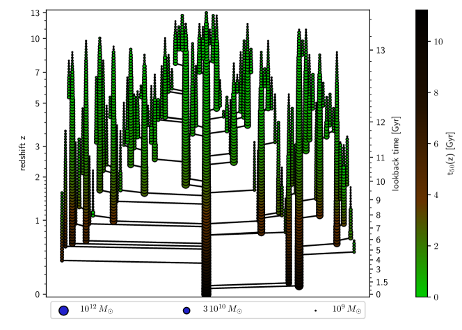
Figure 1: Example of a halo merger tree, obtained with the Monte-Carlo halo merger tree code of Parkinson et al. (2008), where the $z$=0 halo mass is $10^{12}\,{\rm M_{\odot}}$. Each circle represents a halo, where the size of the symbol scales linearly with halo log mass. The colour code, from green to red to brown, scales as $t_{50}=t_{f}-t$, where $t_{f}$ is the lookback time when the most massive progenitor of a halo has half its mass at lookback time $t$. Time flows from top to bottom. The central branch shows the growth of the most massive progenitor. For clarity, only branches above $2\times 10^{9}\,{\rm M_{\odot}}$ and within these, only haloes above $10^{9}\,{\rm M_{\odot}}$ are shown.

Monte-Carlo halo merger trees are designed to generate realistic merger histories of a given halo of mass $M$ at a redshift $z$ (usually 0). These merger trees are built by generating progenitor masses at a higher redshift, and iterating over those progenitors. For each halo of mass $M_{0}$ at redshift $z_{0}$, the mass $M_{1}$ of the main progenitor at redshift $z_{1}$ is drawn according to a probability distribution function that can be written as $P_{1}(M_{1}|M_{0},z_{0},z_{1})$. A secondary progenitor mass can then be drawn following a probability distribution $P_{2}(M_{2}|M_{1},M_{0},z_{0},z_{1})$. For some codes, multiple secondary progenitors can be drawn following $P_{2}(M_{i}|\sum_{j=1}^{i-1}M_{j},M_{0},z_{0},z_{1})$. Monte-Carlo halo merger tree codes handle mass conservation in different ways, either neglecting smooth accretion by imposing $\sum_{j}M_{j}=M_{0}$, or incorporating diffuse mass growth, i.e. $\sum_{j}M_{j}\leq M_{0}$. The difference $\Delta M=M_{0}-\sum_{j}M_{j}$ can be interpreted as smooth accretion or unresolved mergers. This process is iterated to increasingly higher redshifts, thus building the branches of the halo merger tree down to a predefined mass resolution or up to a maximal redshift. Since those probability distributions do not depend on the previous (lower redshift) outcome, the entire process is Markovian.

The first implementations of Monte-Carlo halo merger trees (Lacey & Cole, 1993; Kauffmann & White, 1993) used the extension of the Press & Schechter (1974) model for the cosmic halo mass function, while modern implementations use more accurate probability distribution functions. Jiang & van den Bosch (2014) have recently compared 6 implementations of 4 halo merger tree codes, for $z$=0 halo masses $M_{0}$ ranging from $10^{11}$ to $10^{15}\,h^{-1}\,\rm M_{\odot}$, with branches of mass $>10^{-4}\,M_{0}$. They concluded that the code of Parkinson, Cole & Helly (2008), which is based on extended Press Schechter theory (Bond et al., 1991; Bower, 1991; Lacey & Cole, 1993), with an additional term that is designed to achieve better mass conservation, reproduced best the mass assembly histories, merger rates and unevolved subhalo mass functions measured in cosmological $N$-body simulations with the same cosmological parameters as previously used in the Millennium simulations: $(\Omega_{m},\Omega_{\Lambda},h,\sigma_{8})=(0.25,0.75,0.73,0.9)$, which is close to the WMAP $1^{\rm st}$ year cosmology (Spergel et al., 2003). Parkinson et al. calibrated the two free parameters of their algorithm to match the conditional mass functions, as well as the distribution of the epochs of most recent major mergers, both measured in the Millennium simulation. We therefore adopted the code of Parkinson et al. (2008).

The Parkinson et al. code creates a binary tree with very fine time resolution, so that only the main and one secondary halo are drawn for a given halo mass. This code enables the user to adopt a custom, coarser, output time resolution of the merger tree. Thus, our tree outputs may contain non-binary mergers, but these are built from binary mergers at the fine internal resolution of the code. We chose 101 output timesteps in equal increments of $\log(1\!+\!z)$ from redshift $z=0$ to redshift $z=13$. Our first non-zero redshift is $z=0.0267$, corresponding to a lookback time of 350 Myr.

Figure 1 illustrates the Monte-Carlo halo merger tree obtained with the Parkinson et al. halo merger tree code. While mergers of branches are clearly seen along the main branch, they also occur within the secondary branches. The figure shows the diversity of halo formation times (summed over the progenitors): before being merged into more massive haloes, massive haloes always form early (brown) while low-mass haloes form early (brown) or late (green). A halo can have only one descendant per timestep (halo fragmentation is not allowed). However, the number of progenitors a given halo can have is zero (a newborn halo), one (a quiescent halo), or several (mergers occurring between time outputs).

We ran the Parkinson et al. halo merger tree code with the cosmological parameters of the Millennium simulations, i.e., $(\Omega_{m},\Omega_{\Lambda},h,\sigma_{8})=(0.25,0.75,0.73,0.9)$. We adopted final halo log masses of $\log(M_{0}/{\rm M}_{\odot})=7$ to 14 in steps of 0.025 dex, and a mass resolution $M_{\rm min}=10^{-4}M_{0}$. The minimum halo mass of $10^{7}\,{\rm M_{\odot}}$ is chosen to ensure that we include the halo mass of I Zw 18 (possibly as low as $10^{8.5}\,{\rm M_{\odot}}$ Lelli et al., 2012). By going to such low halo masses, we are assuming that the Parkinson et al. tree code remains valid 4 dex below where it was tested. For each value of $\log M_{0}$, we have run the halo merger tree code 1000 times with different random seeds. In total, we have generated $1000\times[(14-7)/0.025+1]=281$ $000$ halo merger trees.

These merger trees are qualitatively very similar to analogous merger trees extracted from (cosmological) $N$-body simulations. Our Monte-Carlo trees have superior mass resolution in comparison with the halo trees extracted from the MS or even from the MS-II: the final halo masses extend 2 dex lower than the haloes resolved by MS-II with 100 particles, and the progenitors of our haloes have 4 extra dex of resolution, so that our Monte Carlo halo merger trees reach a progenitor mass resolution that is 6 orders of magnitude better than that of the MS-II haloes.

Note that, while the haloes in $N$-body simulations can decrease in mass from one step to the next (because of tidal forces during close interactions), our haloes cannot lose mass, by construction.

2.3 Analytical galaxy formation models

2.3.1 Basic formalism

We first consider very simple galaxy formation models where stellar masses $m_{\rm stars}$ are assigned to haloes with a star formation efficiency (SFE) that depends on halo mass $M$ and redshift $z$, according to

$$m_{\rm stars}\equiv\widetilde{m}(M,z)=f_{\rm b}\,M\,F_{\rm SFE}(M,z)\ ,$$ (1)

where the tilde sign is to denote that this is a model. In equation (1), $f_{\rm b}=\Omega_{\rm b}/\Omega_{\rm m}$ is the universal baryonic fraction ($f_{\rm b}=0.18$ for our adopted $\Omega_{\rm b}=0.045$ as in the Millennium simulations), while $F_{\rm SFE}$ represents the ratio between the stellar mass of a halo and the total mass in baryons expected within the halo. Our analytical models are entirely based on our choice for $F_{\rm SFE}(M,z)$. They predict the stellar mass, but not the gas mass.

We consider a physically-motivated model, as well as two empirical ones based on abundance matching (see Sect. 2.3.3). We also use another empirical model, based on an equation similar to equation (1), but where masses are replaced by mass variations. This use of several different galaxy formation models allows us to gauge the dependence of our results on the uncertainties of galaxy formation.

If one specifies a form for $F_{\rm SFE}(M,z)$, one can derive the stellar mass history of every halo. Following Cattaneo et al. (2011), who pioneered the use of equation (1), and Habouzit et al. (2014), we forbid stellar masses to decrease, i.e. the stellar mass of the (central) galaxy has to be greater or equal to the sum of its galaxy progenitors.

2.3.2 Physical analytical model: Cattaneo et al. (2011) with Gnedin (2000) at the low-mass end

Cattaneo et al. (2011) (hereafter C11) have presented a quasi-physical model for $m(M,z)$ that combines 1) supernova feedback, 2) a gentle cutoff at the high-mass end caused by the virial shock around high-mass haloes (Birnboim & Dekel, 2003; Dekel & Birnboim, 2006), and 3) a sharp cutoff at the low-mass end (motivated by early hydrodynamical simulations of Thoul & Weinberg, 1996) due to the entropy barrier that prevents high entropy gas from collapsing onto its halo (given that its entropy cannot decrease). This is written as $F_{\rm SFE}\propto 1-v_{\rm reion}^{2}/v_{\rm c}^{2}$, where $v_{\rm reion}$ is a constant, while $v_{\rm c}^{2}$ is the squared circular velocity of the halo

$$v_{\rm c}^{2}=\left[{\Delta(z)\over 2}\right]^{1/3}\,\left[H(z)\,G\,M\right]^{2/3}\ ,$$ (2)

where $\Delta(z)$ is the ratio of the mean density within the virial radius to the critical density of the Universe, while $H(z)$ is the Hubble constant.

The supernova feedback prescription of Cattaneo et al. is physically motivated: it is based on the idea that a fraction of the accreted gas that is processed into stars is rapidly ejected as supernova winds, whose velocity matches the virial velocity of the halo and whose energy is assumed to be entirely mechanical and proportional to the remaining stellar mass. This yields $F_{\rm SFE}\propto 1/(1+v_{\rm SN}^{2}/v_{\rm c}^{2})$, where $v_{\rm SN}$ is another constant. At large halo masses, the virial shock quenches the infall of cold gas filaments by heating them up near the virial radius. Star formation in the disc is then limited by the much longer cooling time of the shock-heated gas. This is assumed to yield $F_{\rm SFE}\propto 1/(1+M/M_{\rm shock})$, where $M_{\rm shock}$ is a third constant.

This leads to equation (8) of Cattaneo et al. (2011):

$$F_{\rm SFE}^{\rm C11}(M,z)={1-v_{\rm reion}^{2}/v_{\rm c}^{2}\over 1+M/M_{\rm shock}}\,\left(1+v_{\rm SN}^{2}/v_{\rm c}^{2}\right)^{-1}\ ,$$ (3)

where the constants $v_{\rm reion}$, $v_{\rm SN}$, and $M_{\rm shock}$ respectively represent the minimum circular velocity for gas to overcome the entropy barrier and collapse with the dark matter and subsequently form stars, the impact of supernova feedback, and the characteristic minimum mass for the occurrence of virial shocks. The first term of equation (3) describes the ability to accrete gas, while the second term describes the ability to retain this accreted gas. At high halo masses, galaxy mergers produce galaxies with higher masses than predicted with $F_{\rm SFE}(M,z)$ (see Cattaneo et al., 2011), but the present work focuses on intermediate- and low-mass galaxies.

Given the expected sensitivity of the fraction of VYGs to the form of the threshold of star formation efficiency, $F_{\rm SFE}$, we improve on the model of Cattaneo et al. (2011) by introducing, at the low-mass end, a smoother cutoff, derived from hydrodynamical simulations (Gnedin, 2000; Okamoto, Gao & Theuns, 2008). The accreted mass (disregarding for now the virial shock affecting higher masses) is no longer $m_{\rm accr}=f_{\rm b}M(1-v_{\rm reion}^{2}/v_{\rm c}^{2})$ but instead

$$m_{\rm accr}=\left[1+\left(2^{2/3}-1\right)\left(\frac{v_{\rm reion}}{v_{\rm c}}\right)^{6}\right]^{-3/2}f_{\rm b}\,M\ .$$ (4)

Thus, $v_{\rm reion}$ is no longer the halo circular velocity below which no star formation can occur, but instead the halo circular velocity where the accreted mass is reduced by a factor 2 by the entropy barrier. There is no longer a sharp cutoff of star formation at $v_{\rm c}=v_{\rm reion}$ as in (eq. [3]), but instead the stellar mass increases as $v_{\rm c}^{9}$ (much steeper than the Tully-Fisher relation).

Using equation (4), equation (3) becomes

$$F_{\rm SFE}^{\rm C+G}(M,z)={\left[1+\left(2^{2/3}\!-\!1\right)\,\left(v_{\rm reion}/v_{\rm c}\right)^{6}\right]^{-3/2}\over\left(1+M/M_{\rm shock}\right)\,\left(1+v_{\rm SN}^{2}/v_{\rm c}^{2}\right)}\ .$$ (5)

While the terms for the effects of supernovae and the entropy barrier are respectively motivated by physical principles and hydrodynamical simulations, the term involving the virial shocks is, admittedly, empirical (which is why we dub this model ‘quasi-physical’, but later call it ‘physical’ to distinguish it from the fully empirical models that we will discuss below).

In this ‘Cattaneo+Gnedin’ model (hereafter, C+G), we refer to the values of $v_{\rm reion}$ before and after reionization as $v_{\rm pre-reion}$ and $v_{\rm post-reion}$, respectively. We adopt the following parameters, which produce a good fit to the present-day mass function of galaxies (see Figure 6 below): $v_{\rm SN}=300\,\rm km\,s^{-1}$, $v_{\rm pre-reion}=18\,\rm km\,s^{-1}$, $v_{\rm post-reion}=50\,\rm km\,s^{-1}$, $M_{\rm shock}=10^{12}{\rm M_{\odot}}$. According to equation (4), gas accretion is suppressed by a factor 10 if $v_{\rm c}=0.74\,v_{\rm reion}$. Since $v_{\rm c}=\sigma_{v}/0.7$ for NFW halos (derived from eqs. [22] and [24] of Łokas & Mamon, 2001), $v_{\rm pre-reion}=18\,\rm km\,s^{-1}$ corresponds to a halo temperature of $10\,500\,\rm K$, i.e. the temperature of atomic Hydrogen cooling. Similarly, $v_{\rm post-reion}=50\,\rm km\,s^{-1}$ corresponds to $T=82\,000\,\rm K$. Our adopted value of $M_{\rm shock}$ is double that of Dekel & Birnboim (2006) and 10 per cent lower than the value employed by Cattaneo et al. (2011). Finally, our adopted value of $v_{\rm SN}$ is chosen to roughly fit the $z$=0 stellar mass function.

The effects of these parameters on the stellar mass function is shown in preliminary versions of this work (Mamon et al., 2011, 2012). The baryonic Tully-Fisher relation is well reproduced by the C+G model (Silk & Mamon, 2012).

We could have assumed that the Universe has reionized instantaneously at a fixed redshift $z_{\rm reion}$, somewhere between 6 and 12. Although reionization fronts are thought to have spread fast throughout the Universe (Gnedin & Ostriker, 1997), there is observational evidence that reionization took a time comparable to the age of the Universe at that epoch. This is suggested by the redshift difference between the epoch $z\approx 9$ where the optical depth to neutral Hydrogen was unity (Planck Collaboration et al., 2016) and the latest epoch, $z\approx 6$, when evidence of a substantially neutral intergalactic medium is seen (Becker et al., 2001). For this reason, we have assumed instead that the Universe reionizes stochastically. Thus, for each halo merger tree, we have drawn $\log(1\!+\!z_{\rm reion})$ from a Gaussian of mean corresponding to a median reionization redshift of $\langle z_{\rm reion}\rangle=7.5$ and a standard deviation $\sigma[\log(1\!+\!z_{\rm reion})]=0.05$. This stochastic reionization redshift is applied to all progenitors within a merger tree. We suppose that merging haloes lie in the same region of the Universe and thus are reionized at the same redshift. The mean SFE (only used for illustrative figures, see Fig. 4 below) is then

$$\left\langle F_{\rm SFE}^{\rm C+G}(M,z)\right\rangle = F_{\rm reion}(z)\,F_{\rm SFE-pre}^{\rm C+G}(M,z)$$ (6)

$$+\left[1-F_{\rm reion}(z)\right]\,F_{\rm SFE-post}^{\rm C+G}(M,z)\ ,$$

where $F_{\rm SFE-pre}^{\rm C+G}$ and $F_{\rm SFE-post}^{\rm C+G}$ are the SFEs for $v_{\rm reion}=v_{\rm pre-reion}$ and $v_{\rm reion}=v_{\rm post-reion}$, respectively, while

$$F_{\rm reion}(z)={1\over 2}\,\left\{1+{\rm erf}\left[{\log(1\!+\!z)-\log(1\!+\!\left\langle z_{\rm reion}\right\rangle)\over\sqrt{2}\,\sigma\left[\log\left(1\!+\!z_{\rm reion}\right)\right]}\right]\right\}$$ (7)

is the probability that reionization occurs before redshift $z$. Equation (7) implies that 90 per cent of the reionization occurs between $z=9.3$ and 6.0.

2.3.3 Empirical model: Moster et al. (2013)

The relation between stellar and halo mass can also be determined empirically, by comparing the cumulative distribution function (CDF) of the observed stellar mass function with the CDF of the halo mass function predicted from cosmological $N$-body simulations, a method known as abundance matching (Marinoni & Hudson, 2002).

Moster, Naab & White (2013, hereafter MNW) have proposed the following form for the star formation efficiency:

$$F_{\rm SFE}^{\rm MNW}(M,z)=2\,{N\over f_{\rm b}}\,\left[\left({M\over M_{1}}\right)^{-\beta}+\left({M\over M_{1}}\right)^{\gamma}\right]^{-1}\ ,$$ (8)

where $F_{0}$, $M_{1}$, $\beta$ and $\gamma$ are positive constants. Moster et al. computed the halo and subhalo mass functions in the MS and MS-II rescaled to WMAP-7 cosmological parameters ($\Omega_{\rm m}=0.272$, $h=0.704$, $\sigma_{8}=0.81$). Since subhaloes are tidally stripped, Moster et al. computed the subhalo masses at the time they entered their halo, and accounted for orphan subhaloes that were no longer resolved in the simulations but should have survived given their long expected orbital decay time from dynamical friction. Performing abundance matching at several redshifts from 0 to 4, Moster et al. determined

$$N = 0.0351-0.0247\,z/(1\!+\!z)\ ,$$

$$M_{1} = {\rm dex}\left[11.59+1.195\,z/(1\!+\!z)\right]\ ,$$

$$\beta = 1.376-0.826\,z/(1\!+\!z)\ ,$$

$$\gamma = 0.608+0.329\,z/(1\!+\!z)\ .$$ (9)

2.3.4 Empirical model: Behroozi et al. (2013)

Behroozi, Wechsler & Conroy (2013, hereafter BWC) have also (independently) performed abundance matching, with however several differences as compared to Moster et al. (2013). First, their halo mass functions are derived from a different dissipationless cosmological $N$-body simulation, Bolshoi (Klypin, Trujillo-Gomez & Primack, 2011), with cosmological parameters ($\Omega_{\rm m}=0.27$, $h=0.70$, $\sigma_{8}=0.82$) consistent with WMAP5 (Komatsu et al., 2009). The second difference is the more complex form for $F_{\rm SFE}(M,z)$:

$$F_{\rm SFE}^{\rm BWC}(M,z)=\left({\epsilon M_{1}\over f_{\rm b}M}\right)\,{\rm dex}\left\{f\left[\log\left({M\over M_{1}}\right)\right]\!-\!f(0)\right\},$$ (10)

where

$$f(x)=-\log\left(1+10^{\alpha x}\right)+\delta\,{\left\{\log\left[1+{\rm e}^{x}\right]\right\}^{\gamma}\over 1+\exp\left(10^{-x}\right)}\ .$$ (11)

Behroozi et al. argue that their more refined shape for $F_{\rm SFE}(M,z)$ improves its accuracy by a factor 4.

The third difference with MNW  is that Behroozi et al. fitted their model and the halo+subhalo mass function to, not only the stellar mass function at different redshifts, but also to the dependence with mass of the specific star formation rate at different redshifts, as well as to the evolution of the cosmic star formation rate with redshift. The fourth difference is that the Behroozi et al. model is fit to observational data at sufficiently high redshifts to start probing the epoch of reionization: from 0 to 8 (while MNW  stops at $z=4$). Behroozi et al. derive the halo+subhalo mass function by assuming a model for the dependence with halo/subhalo mass of the fraction of haloes or subhaloes that are subhaloes (which they calibrate at high masses to measurements from simulations).

Their analysis yields the best-fit set of parameters:

$$\epsilon = {\rm dex}\left[-1.777-0.006\,(a\!-\!1)\,\nu-0.119\,(a\!-\!1)\right]\ ,$$

$$M_{1} = {\rm dex}\left\{11.514-\left[1.793\,(a\!-\!1)+0.251\,z\right]\,\nu\right\}\ ,$$

$$\alpha = -1.412+\left[0.731\,(a\!-\!1)\right]\,\nu\ ,$$

$$\delta = 3.508+\left[2.608\,(a\!-\!1)-0.043\,z\right]\,\nu\ ,$$

$$\gamma = 0.316+\left[1.319\,(a\!-\!1)+0.279\,z\right]\,\nu\ ,$$ (12)

where

$$a = {1\over 1\!+\!z}\ ,$$

$$\nu = \exp\left[-{4\over(1\!+\!z)^{2}}\right]\ .$$ (13)

2.3.5 Empirical model: Mutch et al. (2013)

The model of Mutch, Croton & Poole (2013, hereafter MCP) replaces the stellar and halo masses of equation (1) by their time derivatives (see also Moster, Naab & White, 2017):

$${{\rm d}m\over{\rm d}t}=f_{b}{{\rm d}M\over{\rm d}t}\,F_{\rm SFE}^{\rm MCP}(M,z)\ .$$ (14)

Mutch et al. assume lognormal functions for $F_{\rm SFE}(M)$ at given $z$, and we adopt their evolving, “$M_{\rm vir}$”-based model, which in our notation is

$$F_{\rm SFE}^{\rm MCP}(M,z)={\cal E}(z)\exp\left[-\left({\log M\!-\!\log M_{\rm peak}(z)\over\sigma(z)}\right)^{2}\right],$$ (15)

where

$${\cal E}(z) = 0.90\,(1\!+\!z)^{-0.74}\ ,$$

$$\log M_{\rm peak}(z) = 11.6\,(1\!+\!z)^{0.03}\ ,$$

$$\sigma(z) = 0.56\,(1\!+\!z)^{0.25}\ .$$ (16)

The parameters of the MCP  model were fit to constrain both the $z$=0 SMHM and the stellar mass functions at redshifts up to $z=3$, split between red and blue galaxies. Mutch et al. obtained these parameters by running their model on halo merger trees from the MS, with the same cosmological parameters (but they express their halo masses using $h=0.7$ instead of $h=0.73$, a 4 per cent relative difference that we, hereafter, neglect).

The MCP model of equation (14) has the advantage of producing, through stellar mass growth, a natural scatter in the SMHM from the stochasticity of the halo mass growth. Moreover, by construction, stellar mass cannot decrease in the MCP model. Since the MCP model is based on time derivatives, it does not predict a minimal stellar mass, but a minimal mass growth. Therefore, higher stellar mass growth can only be caused by mergers. We decreased their normalization ${\cal E}$ by 30 per cent (as they suggest) to account for the loss of stellar mass by supernova explosions.

2.3.6 Comparison of the analytical galaxy formation models

Table 1: Galaxy formation models

Abbreviation	Reference	Nature	Relation	Calibration	Power	Cosmology				$z$=0 haloes			Halo merger trees
				max $z$	spectrum	$\Omega_{\rm m}$	$h$	$\sigma_{8}$		$\log M_{0}^{\rm min}$	number		method	resolution
(1)	(2)	(3)	(4)	(5)	(6)	(7)	(8)	(9)		(10)	(11)		(12)	(13)
C+G	Cattaneo+11	physical	$m=f(M,z)$	0.1	CDM	0.28	0.70	0.82		7	281 000		Monte-Carlo	$10^{-4}$
MNW	Moster+13	empirical	$m=f(M,z)$	4	CDM	0.27	0.70	0.81		7	281 000		Monte-Carlo	$10^{-4}$
BWC	Behroozi+13	empirical	$m=f(M,z)$	8	CDM	0.27	0.70	0.82		7	281 000		Monte-Carlo	$10^{-4}$
MCP	Mutch+13	empirical	$\dot{m}=f(\dot{M},z)$	3	CDM	0.25	0.70	0.90		7	281 000		Monte-Carlo	$10^{-4}$
Henriques	Henriques+15	SAM	complex	3	CDM	0.31	0.67	0.83		7.8	1 169 786		MS-II	$10^{9}\,\rm M_{\odot}$
Henriques	Henriques+15	SAM	complex	3	CDM	0.31	0.67	0.83		9.9	1 514 920		MS	$10^{11.1}\,\rm M_{\odot}$
Menci	Menci+08,14	SAM	complex	none	CDM	0.30	0.70	0.90		9.5	2 100		Monte-Carlo	$10^{7.7}\,\rm M_{\odot}$
Menci	Menci+08,14	SAM	complex	none	WDM	0.30	0.70	0.90		9.5	2 100		Monte-Carlo	$10^{7.7}\,\rm M_{\odot}$

Notes: the columns are as follows. (1): model abbreviation used in text; (2): reference; (3): nature (quasi-physical analytical, empirical analytical, or semi-analytical [SAM]); (4): relation between stellar and halo mass; (5) maximum redshift for calibration to observational data; (6): primordial power spectrum; (7): cosmological density parameter; (8): dimensionless Hubble constant; (9): standard deviation of primordial density fluctuations at scales of $8\,h^{-1}\,\rm Mpc$ (both linearly extrapolated to $z=0$); (10): minimum final halo log mass (solar units); (11): number of Monte Carlo merger trees or of $z$=0 haloes more massive than $10^{9}M_{\odot}$ (for the Henriques SAMs); (12): tree method; (13): minimal halo mass in tree (the first four rows are relative to the $z$=0 mass; the values for the Henriques SAMs are for haloes resolved with 100 particles). The first five models are the major ones of this study, while the latter three are for specific analyses.

Table 1 summarizes the analytical models used here, as well as the semi-analytical models presented in Sect. 2.4. The cosmological parameters are those of the simulations that were used to calibrate to the observations.

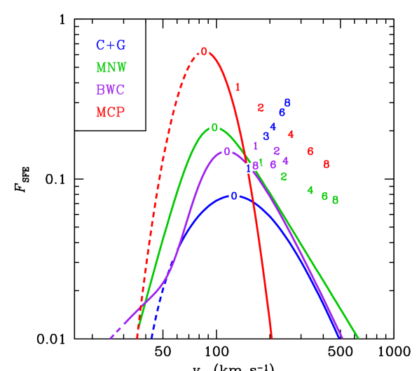
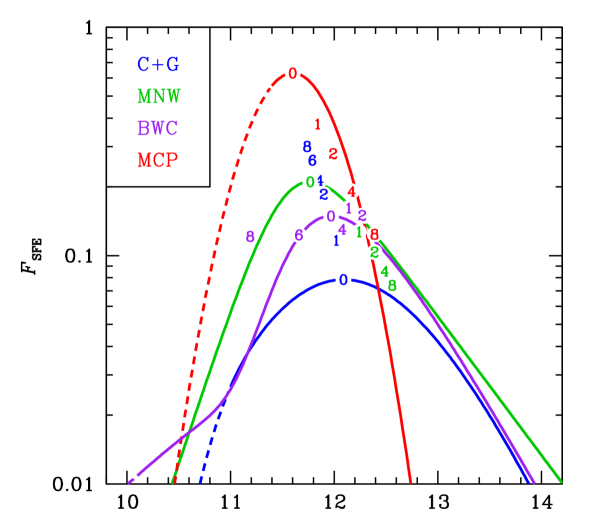
Figure 2: Star formation efficiency, $F_{\rm SFE}$, of our analytical galaxy formation models versus halo circular velocity (top) and mass (bottom) at $z=0$. The blue, green and purple curves respectively show $F_{\rm SFE}=m/(f_{\rm b}M)$ for models C+G (Cattaneo et al., 2011 with Gnedin, 2000, eqs. [5], [6] and [7]), MNW (Moster et al., 2013, eqs. [8] and [9]), and BWC (Behroozi et al., 2013, eqs. [10], [11], [12], and [13]). For model MCP (Mutch et al., 2013, eqs. [15] and [16], red curve), $F_{\rm SFE}=0.7\,\dot{m}/(f_{\rm b}\dot{M})$. The dashed portions of the curves indicate where the models are extrapolations. The numbers indicate the position of the peak star formation efficiency at the corresponding redshift.

Figure 2 shows the comparison of the 4 models at redshifts $z=0$ and the peak SFE at redshifts 1, 2, 4, 6, and 8. Note that only the BWC model was fit by the authors up to $z=8$. The four models agree to first order, although there are some notable differences. While the MCP model, by construction, has a symmetric $F_{\rm SFE}$ in $\log v_{\rm circ}$ and in $\log M$, all other models are asymmetric, with a relatively faster decrease of SFE at low circular velocity or halo masses, except for the shallow low-end tail in the BWC model at low redshift. But recall that the $F_{\rm SFE}$ of the MCP model is defined in a different fashion (eq. [14] vs. eq. [1]).

The peak SFE decreases with time in the C+G  model, increases with time in the MNW  and MCP models, and is roughly independent of redshift in the BWC  model. The circular velocity (respectively, halo mass) where this peak SFE is reached decreases (increases) slightly with time in the C+G  model, increases sharply with time in the MNW and MCP models, and increases moderately with time in the BWC model up to $z=4$ ($z=2$) then reverses and decreases with time increasingly faster.

At the high-mass end, the decrease of $F_{\rm SFE}$ with halo circular velocity at $z=0$ follows a similar slope (–2.5) in the physical C+G and empirical BWC models, while the MNW model shows a somewhat shallower decrease (slope –2). In contrast, the MCP model shows an increasingly rapid decrease, with a much steeper slope, close to $-9$ at 1 percent of peak SFE.

At the low-mass end, the rise of $F_{\rm SFE}$ with halo circular velocity is fastest for the C+G  model ($F_{\rm SFE}$ rises as $v_{\rm c}^{9}$ according to eq. [5]) and the MCP model, for which the slope is even steeper than 9 at levels where SFE is at 1 percent of its peak value. At $z=0$, the MNW  model gives a low-end slope of 4.1 for $F_{\rm SFE}$ vs. $v_{\rm c}$, the BWC  model has a much shallower slope of 1.2, while that of the MCP model slowly tends to infinity (because of the lognormal SFE vs. halo mass), and at 1 per cent of the peak SFE, the slope is 3.3 at $z=0$ and 2.1 at $z=5$. At higher redshifts, while the C+G  model retains the same steep slopes at the low-end of $F_{\rm SFE}$ vs. $v_{\rm c}$, the MNW  model becomes shallower with increasing redshift, while the BWC  model becomes steeper with redshift. Thus, at $z=5$, the BWC’s $F_{\rm SFE}$ vs. $v_{\rm c}$ relation is steeper (slope 2.9) than that of MNW (slope 2.1).

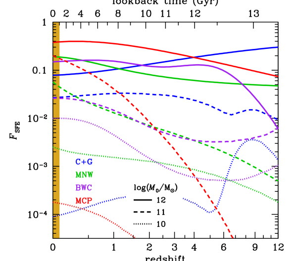
Figure 3: Evolution of the star formation efficiency, at fixed halo mass, for the four analytical models (see Fig. 2), for final log halo masses of 10, 11 and 12 (solar units). The shaded gold region highlights the final Gyr.

Figure 3 compares directly the evolution of $F_{\rm SFE}$ between the 4 analytical models. In particular, the C+G model has decreasing SFE in the last 8 or more Gyr (depending on final halo mass), whereas the BWC model shows a flat SFE in the last Gyr, while the MNW and MCP models appear to have increasing SFE at all times. In models with $F_{\rm SFE}$ that decrease with time such as C+G and BWC at late times, a galaxy whose halo mass remains constant in time (from an unlucky lack of mergers that would otherwise make it grow) will see a decreasing $F_{\rm SFE}$ at constant $M$, hence a decrease in stellar mass. In these cases, our forcing the stellar mass not to decrease comes into effect. In contrast, the MCP model, based on time derivatives, is the only one where stellar mass is guaranteed to never decrease in time.

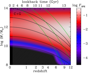
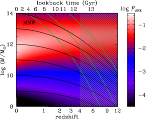
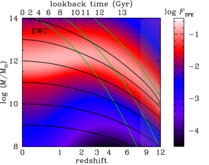
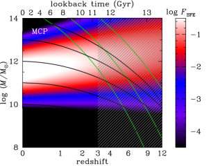
Figure 4: Variation of the star formation efficiency with halo mass and epoch for the four analytical models (see Fig. 2). The slowly decreasing black curves indicate the median mass assembly of the main progenitors of the haloes. The 3 rapidly decreasing green curves indicate 2, 3 and 5$\,\sigma$ fluctuations (going upwards), so that the upper right portions of each panel are irrelevant, since such massive haloes are extremely rare at high redshift. The grey hatched regions indicate the redshifts where the models are extrapolated. The colour scales of the 4 panels are identical. Given the different definition of $F_{\rm SFE}$ of the MCP model, it is not directly comparable to the other three models. Note the different cosmologies used for each model to link lookback time and redshift.

Figure 4 illustrates how $F_{\rm SFE}$ varies with both halo mass and redshift for each of the 4 analytical models. Naturally, the essential features of Figures 2 and 3 are recovered: The higher peak $F_{\rm SFE}$ at low redshift for the MCP model shows as a whiter colour in Figure 4. The sharp drops of $F_{\rm SFE}$ at low halo mass of the MCP model at $z=0$ seen in Figure 2 are visible here as rapid transitions to black colour at all redshifts (again, recall that $F_{\rm SFE}$ is defined in a different fashion for the MCP model). This is also the case for the C+G model. However, at high mass, the drop of $F_{\rm SFE}$ with mass at $z=0$ is only pronounced for the MCP model (again seen at all redshifts).

Given that the intergalactic medium should be fairly cold before reionization and then is gradually heated by photoionization from galaxies and quasars, one expects that star formation at low circular velocities (masses) should only occur at higher redshifts. The C+G model has this low-mass effect built-in, with $v_{\rm post-reion}>v_{\rm pre-reion}$. But, a striking feature of Figure 4 is that the BWC model is the only one for which the halo mass at peak $F_{\rm SFE}$ has a clear maximum at $z=3$ (see also Fig. 2). In other words, the BWC empirical model suggests that the effects of photoionization apply to all masses, as the entire $F_{\rm SFE}(M)$ is shifted to lower masses at higher redshifts. This “reionization of the Universe” feature strongly seen in BWC and also visible at the low end of the C+G model, is not seen in the MNW or MCP models, because they were tuned to observations that did not extend far enough in redshift, so the extrapolation to higher redshifts (grey shaded regions of Fig. 4) is incorrect.

Figure 4 also expands on Figure 3 by showing that not only do models C+G and BWC show halo masses with decreasing $F_{\rm SFE}$, but models MNW and MCP also show decreasing $F_{\rm SFE}$ for high halo masses ($\log\,(M/{\rm M}_{\odot})\mathrel{\hbox{\hbox to0.0pt{\hbox{\lower 4.0pt\hbox{$\sim$}}\hss}\hbox{$>$}}}12$).

Moreover, Figure 4 shows that the BWC model is the only one that displays a decrease at late times of the lower envelope of the halo masses with efficient star formation. By definition, VYGs require a very late jump in stellar mass, which should usually come together with a sudden jump in halo mass (we will discuss this in more detail in Sect. 5.2.2). One would therefore expect that, contrary to the other 3 analytical models, the BWC model will lead to fewer VYGs, because, at relatively late times, the SFE will increase as the halo mass rises, causing star formation in the last few Gyr before $z=0.08$, which should make it difficult to have a very young stellar population at $z=0$.

2.3.7 Galaxy merging in analytical models

The galaxies in our analytical models can grow in a quiescent mode, via equation (1) (or (eq. [14] for the MCP model), or by galaxy mergers. The new stellar mass of the galaxy in halo $i$ of mass $M_{i}$ is the maximum value of the masses given by the quiescent growth and by the growth by galaxy mergers:

$$m(i,s) \equiv {\rm Max}\left[\widetilde{m}(M_{i},s),\sum_{\rm prog}m_{\rm old}\right]$$ (17)

$$= {\rm Max}\left[\widetilde{m}(M_{i},s),\sum_{j}m(j,s\!-\!1)\right]\ ,$$

where the $j$s are the indices of the progenitors of halo $i$ from the previous timestep, while $\widetilde{m}(M,s)$ is the model stellar mass at timestep $s$ for a galaxy in a halo of mass $M$ (eq. [1]). For the MCP model, the model mass in equation (17) is understood to be $\widetilde{m}=m_{\rm old}+f_{\rm b}\,F_{\rm SFE}(M,z)\,\Delta M$.

While our different analytical galaxy formation models generally predict different stellar masses associated to both progenitors, they are run on the same halo merger trees, hence galaxy mergers occur at the same time in each model (but involve different stellar masses).

Our analytical models cannot directly handle possible starbursts in merging gas-rich galaxies. Instead, we have implemented 2 different schemes to handle halo mergers that roughly reproduce the situations of gas-rich and gas-poor mergers.

In our bursty galaxy merging scheme, we delay subhalo (galaxy) merging by a suitable dynamical friction time, $t_{\rm df}$ (see eq. [19] below), measured from the last time when the two haloes were distinct in the halo merger tree. We do not model the subhalo mass evolution (its decrease by tidal stripping), and thus the satellite galaxy that originated from this branch has a constant stellar mass until it merges with the central galaxy. We do not consider satellite galaxies that merge later than $z=0$ because of disk storage issues and because our main focus is on central galaxies.

With bursty galaxy merging, the central galaxy sees a boost in stellar mass at the time of the halo merger, when the first term within the brackets of equation (17) dominates the second one. It recovers the masses of the satellites only after the dynamical friction time has elapsed. This scheme thus creates a burst of star formation at the first pericentre. Note that hydrodynamical simulations of merging galaxies indicate that while a starburst occurs at first pericentre, there is usually another stronger one at the second pericentre, when the 2 galaxies complete their merger (e.g. Cox et al., 2008; Di Matteo et al., 2008), but this cannot be modelled in our code.

In our quiet galaxy merging scheme, we not only delay the galaxy merger by the dynamical friction time, but we also modify the stellar mass at the time of the halo merger (eq. [17]). For this, we subtract from the new halo mass the total mass $\sum M_{k}$ of all the branches that 1) merge at the current timestep or before, and 2) contain galaxies turning into satellites that do not have time to merge into the central galaxy (after dynamical friction) by the current timestep. The new central galaxy mass is then

$$m(i,s)={\rm Max}\left[\widetilde{m}\left(M_{i}\!-\!\sum M_{k},s\right),\sum_{j}m(j,s\!-\!1)\right]\ ,$$ (18)

where the $j$s are again (as in the bursty merger scheme) the indices of the progenitors of halo $i$ from the previous timestep. With equation (18), there is no boost of stellar mass at the time of the halo merger, hence our quiet scheme represents well the situation of dry galaxy mergers.

Following Jiang et al. (2008), we adopt a dynamical friction time of

$$t_{\rm df}(M_{1},M_{2},z)=A\,\frac{M_{1}/M_{2}}{\ln(1+M_{1}/M_{2})}\,{r_{\rm v}\over v_{\rm v}}\ ,$$ (19)

where $r_{\rm v}/v_{\rm v}=\sqrt{2/\Delta(z)}/H(z)$ is the orbital circular time divided by $2{\rm\pi}$ at radius $r_{\rm v}$, with $\Delta(z)$ being the overdensity relative to critical for collapse, for which we adopt the approximation of Bryan & Norman (1998). In equation (19), $A$ is a dimensionless constant that depends on orbit eccentricity. There is some debate on the value of $A$. Jiang et al. (2008) calibrated $A=1.43$ using hydrodynamical cosmological simulations, while other values of $A$ range from 0.58 (Springel et al., 2001) to 2.34 (De Lucia & Blaizot, 2007; Guo et al., 2011; Henriques et al., 2015), with the latter value adjusted to better fit the observed galaxy optical luminosity functions with SAMs. We adopted $A=2.34$ to be consistent with the Henriques SAM and the MNW model.

The dynamical friction time of equation (19) is always longer than a few Gyr. It is shortest for equal mass mergers, for which it is $A/(\ln 2)\,\sqrt{2/\Delta}/H>0.36/H$ at all times, and is $>0.47/H$ and $>6.2\,\rm Gyr$ for lookback times less than 1 Gyr (where we assumed the Millennium cosmology). Therefore, galaxies merge several Gyr (hence many timesteps) after their halos merge.

Since our focus is on VYGs, which should be gas-rich, we adopt the bursty merging as our primary galaxy merging scheme, but will later compare to the quiet scheme.

2.3.8 Practical issues for the analytical models run on the Monte-Carlo merger trees

We first run the halo merger tree code, which writes the trees to files. The analytical galaxy formation models are applied using a second code that is run on each halo within each tree. This code starts at the highest redshift of $z=13$ and works forward in time, producing the stellar mass assembly history within the halo mass assembly history. We assign initial stellar masses to each halo according to the model mass of equation (1) for the first three models, and to zero for the MCP model.

We analyse the stellar mass history summed up over all progenitors of a particular halo at redshift zero. Had we only considered the growth of stellar mass of the main progenitor, we would have measured the stellar mass assembly instead of the star formation history. We discard all $z$=0 stellar masses below $10^{3}\,{\rm M_{\odot}}$.

Ideally, since the analytical models have been calibrated on halo mass functions from different cosmologies, it would have been best for us to run the halo merger tree code separately for each of our analytical models, adapting the cosmological parameters on which each model was built. This proved difficult to do in practice because of the large disc space required, hence we ran the halo merger tree code only once, i.e. with the same cosmological parameters (see end of Sect. 2.2) for all 4 analytical models.

The different models employ slightly different definitions of halo mass. Our Monte-Carlo halo merger tree is built with the Parkinson et al. (2008) algorithm, which is based on masses of the Friends of Friends halo membership in the cosmological simulation (S. Cole, private communication). However, in the halo to stellar mass relations obtained from the empirical abundance matching technique, the halo mass is defined at the spherical overdensity of 200 times critical (MNW) or at Bryan & Norman’s (1998) virial value (BWC, MCP). The mass used with the C+G model is simply that of the Monte-Carlo halo merger tree, on which the model parameters were roughly calibrated, with no pre-calibration on halo mass functions. These inconsistencies in the mass definition should have no significant effect on the resulting analysis (e.g., $\log(M_{\rm vir}/M_{200})$ is only 0.1).

2.4 Semi-analytical galaxy formation models

We also considered two semi-analytical models (SAMs) of galaxy formation. In SAMs, galaxies are modelled as discs plus bulges, each with their characteristic sizes. These codes include complex physical recipes to incorporate gas cooling, star formation, stellar evolution, feedback from supernovae and active galactic nuclei (AGN). These models should be more realistic than the physical analytical models, in particular because they usually model the galaxy positions from those of the subhaloes in the Millennium simulations. However, nearly all SAMs fail to reproduce many of the relations observed for galaxies, while the empirical analytical models are calibrated to these observations.

2.4.1 Henriques et al. (2015)

We first analysed the recent, state-of-the-art SAM of Henriques et al. (2015) that they ran on the halo merger trees of the MS-II, rescaled to the Planck cosmology. The Henriques SAM continues the series of SAMs developed by the Munich team (Croton et al., 2006; De Lucia & Blaizot, 2007; Guo et al., 2011). It also includes ram pressure stripping of satellites in cluster-mass haloes and the formulation of Gnedin (2000) (eq. [4]) to prevent gas accretion on low-mass haloes.

Henriques et al. tuned the free parameters of their model to match as best as possible the $z=0$ to 3 observations of the stellar mass functions and the fractions of passive galaxies. Such a tuning solves several problems in previous implementations of the Munich model. In particular, low-mass galaxies no longer form too early (in contrast with Guo et al.), thanks to longer timescales for the galactic winds to fall back into the discs they originated from.

We extracted from the Henriques2015a table of the Virgo – Millennium database of the German Astrophysical Virtual Observatory (GAVO) the following parameters: the halo mass (corresponding to $M_{200}$) centralMvir, stellar mass stellarMass, and the mean (mass-weighted) age massweightedAge, all at $z=0$ with $m>10^{6}\,{\rm M_{\odot}}$. This extraction yielded $1\,175\,987$ galaxies. We, hereafter, refer to this virtual catalogue and the corresponding SAM model as Henriques. Since the analytical models described above fail to consider satellite galaxies, we limit the Henriques catalogue to the central galaxies.

2.4.2 Menci et al. (2008)

Finally, we considered a second SAM, by Menci et al. (2008), where the baryonic physics is built on top of Monte-Carlo halo merger trees. We chose this SAM, because it has been run on two sets of merger trees: one (Menci et al., 2008) for the $\Lambda$CDM cosmology (with $\Omega_{\rm m}=0.3$, $h=0.7$, $\Omega_{\rm b}=0.04$, and $\sigma_{8}=0.9$) and another (Menci, Fiore & Lamastra, 2012; Calura, Menci & Gallazzi, 2014; Menci et al., 2014) for a $\Lambda$ Warm Dark Matter ($\Lambda$WDM or simply WDM) cosmology. We will only discuss this SAM in the context of estimating the effects of WDM on the fraction of VYGs.

WDM is analogous to $\Lambda$CDM, but with the power spectrum truncated at high wavenumbers, corresponding to scales below $\sim$ 1 Mpc, as expected for a $m_{\chi}\sim 0.75$ keV thermal relic particle. Note that this choice for $m_{\chi}$ is fairly extreme, as the observed abundance of dwarf galaxies around the Milky Way leads to $m_{\chi}>2.3\,\rm keV$ (Polisensky & Ricotti, 2011; Menci et al., 2016). This low value of $m_{\chi}$ sets an upper limit to the effects of the suppression of primordial density fluctuations at high wavenumber.

For both $\Lambda$CDM and $\Lambda$WDM cosmologies, the merger trees were run using 21 final, equal-spaced halo log masses ($9.5<\log(M_{0}/{\rm M}_{\odot})\leq 14.5$), with a mass resolution of $5\times 10^{7}\,{\rm M_{\odot}}$ for all final halo masses $M_{0}$. Each $z$=0 halo mass was run 100 times, leading to a total of 2100 trees (see Table 1).

In this SAM, gas is converted into stars through two main channels: a quiescent accretion mode, occurring on long timescales ($\sim$ 1 Gyr), and an interaction-driven mode, where gas – destabilized during major and minor mergers and fly-by events – turns into stars on shorter timescales (typically $\sim 10^{7}$ yr). AGN activity triggered by galaxy interactions and the related feedback processes are also included.

The Menci et al. SAM was run on the CDM and WDM trees with the exact same recipes and parameters for the baryonic physics. We do not include it in our standard analyses and figures, so as not to overcrowd our figures, given that it uses 100 times fewer trees than our standard ones and the lower mass ones are poorly resolved, and is a much less used SAM than that of Henriques et al. (2015), whose output is publicly available, and which has the additional advantage of being calibrated to the stellar mass functions at redshifts up to 3.

3 Tests of the models

3.1 Stellar versus halo mass

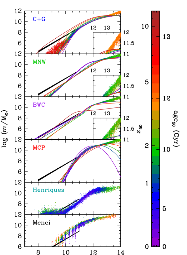
Figure 5: Stellar mass versus halo mass at $z=0$ for the four analytical models (with bursty galaxy merging, top panels, see Fig. 2) and for the SAMs of Henriques and Menci (bottom 2 panels), restricted to centrals with galaxy stellar masses $m>10^{6}\,{\rm M_{\odot}}$ for lack of mass resolution). Each point corresponds to a galaxy extracted from the analytical or semi-analytical models run on the halo merger trees. The points are colour-coded by the median (analytical models) or mean (Henriques SAM) redshift, $z_{50}$, and are plotted in order of decreasing age, with violet colours for the galaxies younger than 1.3 Gyr. For clarity, only 500 galaxies are shown per 0.25 dex halo mass interval. The curves show the stellar mass – halo mass relations directly predicted by the analytical models, with equation (1) for the C+G, MNW, and BWC models and equation (14) for the MCP model, using the star formation efficiencies illustrated in Fig. 2. These curves are given at redshifts 0, 1, 2, 5, and 10, following the same colour code as for $z_{50}$. The insets show 4$\times$ vertical zooms of the high-mass end. The black lines show the observations of isolated dwarf irregular galaxies compiled by Read et al. (2017), with uncertainties illustrated by the line thickness.

In this section, we test our analytical models, by analysing the $z$=0 stellar masses ($m$), halo masses ($M$), and the redshift $z_{50}$ (the corresponding stellar age or lookback time, is called $\rm age_{50}$) when half the mass in stars is formed. For the Henriques SAM, which does not easily provide the epochs when half the stellar mass is formed, we consider instead the mass-weighted mean age of the stellar population, which we also denote as $z_{50}$.

The stellar mass – halo mass (SMHM) relation is a fundamental test of galaxy formation models. Figure 5 illustrates the SMHM, according to the 4 analytical models as well as the Henriques and Menci SAMs, and how galaxy ages depend on their location in the SMHM relation. Note that the Menci SAM uses 0.25 dex steps of $\log\,(M/{\rm M}_{\odot})$, but their output is shown at $z=0.12$ instead of $z=0$, which leads to somewhat less discretization.

The first aspect to note is that only the BWC model leads to an SMHM that matches well the observations of 11 nearby, highly-inclined, isolated dwarf irregulars (black line in Fig. 5) as compiled by Read et al. (2017). The C+G, MNW, and especially MCP models predict lower stellar masses at given halo mass than observed by Read et al., as also does the Henriques SAM. On the other hand, the Menci SAM predicts higher stellar masses at given halo masses than found by Read et al..

The better match to observations with the BWC model appears to be a consequence of its inclusion of a change in slope of the SMHM at the low end, which was not incorporated in the other analytical models. Interestingly, Read et al. (2017) noticed that the SMHM they obtained for their sample of 11 dwarf galaxies follows the SMHM related predicted from the extrapolation to low masses of the abundance matching of the SDSS stellar mass function (SMF) of Baldry et al. (2008) with the cosmic halo mass function. This explains the agreement between their SMHM and that found for BWC, who had also used the SMF of Baldry et al. (2008). In comparison, MNW adopted the same SMF, but adopted a too restrictive single-slope low-end SMHM parameterization. Finally, MCP adopted a different set of SMFs.

The second interesting feature is that the most massive galaxies have formed their stars earlier than the other galaxies (except for the very low-mass galaxies in the C+G model), i.e. one is witnessing downsizing. In contrast the MNW, Menci, and especially the C+G model also predict that the smallest galaxies are old, i.e. upsizing. We will analyse in more detail in Sect. 3.3 how the typical stellar ages of galaxies vary with their $z$=0 stellar mass.

The third interesting aspect of Fig. 5 is that, at intermediate masses, the galaxy stellar masses derived by running the analytical models on the Monte-Carlo halo merger trees (points) are often close to those directly obtained from the models for the redshift corresponding to $z_{50}$ (curves of similar colour). However, at the high-mass end, the stellar masses predicted from running the models on our halo merger trees are greater than those predicted by these two models at $z=z_{50}$ (or at any $z$). For the C+G, MNW, and BWC models, this extra stellar mass at high halo mass, which is clearly seen in the 3 corresponding insets of Fig. 5, suggests that we are in a regime where the analytical stellar mass decreases in time, which our implementation forbids (see end of Sect. 2.3.6). In Figure 4, the ridge of highest SFE occurs at decreasing halo mass at later times before $z=0$, except in the C+G model (where it is roughly constant). However, in this physical C+G model, galaxy mergers can boost the stellar mass beyond the analytical prediction (Cattaneo et al., 2011). Thus, the C+G model highlights the role of mergers at high masses, while showing negligible effects of mergers at lower masses, where the analytical prediction matches well the outcome of the model run on the halo merger trees. The importance of mergers at high masses was previously noted by Guo & White (2008) and Hopkins et al. (2010), who studied the merger rates of galaxies, by Cattaneo et al. (2011) who studied (at better mass resolution) the fraction of stellar mass acquired by mergers, as well as by Bernardi et al. (2011) who analyzed the observations of galaxy properties.

The fourth interesting feature of Figure 5 is that the scatter in the SMHM relation strongly depends on the model. The BWC  and MNW models produce virtually no scatter for halo mass below $10^{12}\,{\rm M_{\odot}}$. In contrast, the C+G model and Menci SAM produce a large scatter in the SMHM relation at low mass. The Henriques SAM produces scatter at both low mass (where mass resolution effects become significant) and high mass (perhaps from the stochasticity of galaxy mergers). While the scatter of the stellar mass of central galaxies in the Henriques, and Menci SAMs are low at intermediate halo masses, it is even lower in the EAGLE hydrodynamical simulations (Guo et al., 2016). The large scatter in the C+G SMHM is clearly due to its higher SFE of low-mass haloes before reionization (see Fig. 4) combined with the stochasticity in recombination epochs in the C+G model. The MCP  model produces some scatter at all masses, as expected from its use of mass evolution rates instead of masses themselves.

3.2 Stellar mass function

In theory, the SMF, ${\rm d}n/{\rm d}m$, can be estimated by integrating over the cosmic $z$=0 halo mass function (known from cosmological simulations), ${\rm d}n/{\rm d}M$:

$${{\rm d}n\over{\rm d}\log m} = \int{\rm d}\log M\,{{\rm d}^{2}n\over{\rm d}\log M\,{\rm d}\log m}$$ (20)

$$= \int{\rm d}\log M\,\left({{\rm d}n\over{\rm d}\log M}\right)\,\left({{\rm d}n\over{\rm d}\log m}\right)_{M}\ .$$

Our choice of equal numbers of haloes (trees) in logarithmic bins of mass produces an unrealistic halo mass function and would thus lead to an unrealistic galaxy SMF. We can nevertheless compute the SMF (in bins $j$ of log stellar mass) as a sum over bins ($k$) of halo mass, by normalizing our flat halo log mass function by the cosmic halo mass function. We thus weight the galaxies $i$ as the ratio of the $z$=0 cosmic halo mass function to the available $z$=0 halo mass function returned from the Monte-Carlo trees, i.e.

$$w_{i}(M_{k})={\left({\rm d}n/{\rm d}\log M\right)_{M=M_{k}}\over\Delta n/\Delta\log M_{k}}\ .$$ (21)

We can then write the measured SMF in bins of constant $\Delta\log m_{j}$ as

$$g(\log m_{j}) \!\!\!\!\equiv\!\!\!\! \left({{\rm d}n\over{\rm d}\log m}\right)_{m=m_{j}}$$ (22)

$$\!\!\!\!=\!\!\!\! \Delta\log M_{k}\sum_{k}\left({\Delta n\over\Delta\log M_{k}}\right)w_{i}(M_{k})\left({\Delta n\over\Delta\log m_{j}}\right)_{k}$$

$$\!\!\!\!=\!\!\!\! {1\over\Delta\log m_{j}}\,\sum_{i\in j}w_{i}(M_{k})\ .$$

The second equality of equation (22) makes use of equations (20) and (21) and of the constant value of $\Delta\log M_{k}$.

We adopted the $z$=0 cosmic halo mass function of Warren et al. (2006), computed using HMFCalc (Murray, Power & Robotham, 2013) with the cosmological parameters used in the Millennium Simulations, and for an overdensity of 200 relative to critical.

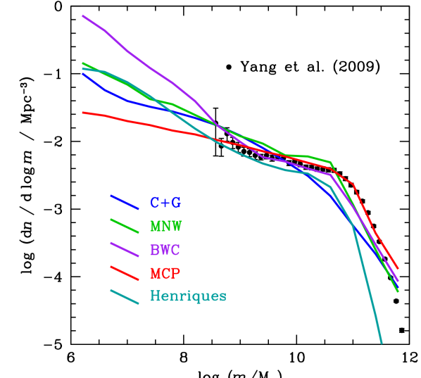
Figure 6: Galaxy stellar mass functions at $z=0$ for the different galaxy formation models: the 4 analytical models (with bursty galaxy merging, see Fig. 2), as well as for the semi-analytical model of Henriques et al. (2015, cyan), for centrals only. The symbols represent the observed central galaxy stellar mass function of Yang et al. (2009), converted to $h=0.7$ and to the Chabrier (2003) initial mass function.

The resultant $z$=0 galaxy SMFs produced by our Monte-Carlo runs for the analytical models are shown in Figure 6, as well as that of the Henriques SAM (restricted to central galaxies) and the observed central galaxy stellar mass function of Yang, Mo & van den Bosch (2009). The figure indicates that the C+G model fails to reproduce the knee of the SMF at $\log(m/{\rm M_{\odot}})\simeq 10.8$. In the range $7\leq\log\,(m/{\rm M}_{\odot})\leq 8$, the logarithmic slopes of the model SMFs are $\approx-1.28$, –1.36, –1.66, $-1.18$, and $-1.51$ for the C+G, MNW, BWC, MCP, and Henriques models, respectively. In comparison, the slope of the observed SMF of Yang et al. is $\approx-1.65$ at $8.7\leq\log(m/{\rm M_{\odot}})\leq 9.3$. Hence, the observed low-end slope is best (worst) matched by the BWC (MCP) model. With the quiet galaxy merging scheme, the SMFs from the analytical models are similar, but shifted down by 0.4 dex, thus matching less well the observed one.

3.3 Age versus mass

We now study how the epoch, $z_{50}$, when half the $z$=0 stellar mass is formed in galaxies varies with the $z$=0 stellar mass. This is illustrated in Figure 7 for the four analytical models of $F_{\rm SFE}(M,z)$, as well as for the Henriques SAM (for which the redshift corresponds to the arithmetic mean age of the stellar population of the galaxy).

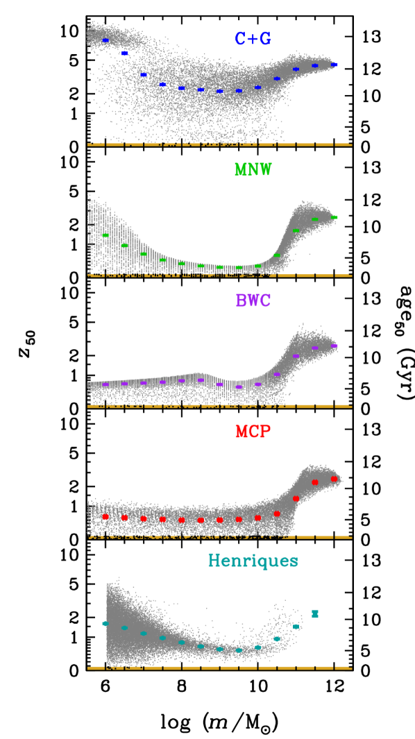
Figure 7: Typical redshift of star formation versus galaxy stellar mass for the analytical models with bursty galaxy merging (median redshifts) and for the central galaxies in the Henriques semi-analytical model (arithmetic mean redshifts). The corresponding ages are shown on the right axis. The grey points show a random subset of 20 000 galaxies. The large coloured symbols show the means (Henriques) or weighted means (other models, eq. [21]) of $\log(1\!+\!z_{50})$, while the error bars display the uncertainties ($\sigma/\sqrt{N}$ for Henriques, and using 1000 bootstraps for the other models). The gold shaded regions indicate ages less than 1 Gyr, and the very young galaxies (from the same random subset) are highlighted as darker and thicker points.

All models show downsizing at the high-mass end, where $z_{50}$ increases with stellar mass. This is due to the negative slope of the SFE - halo mass relations at high halo masses (Fig. 2): the galaxies with the highest stellar masses today live in high mass haloes that grow faster than low-mass ones (van den Bosch, 2002 and black curves of Fig. 4) and also faster than the mass of the peak SFE (whiter ridges in Fig. 4), leading to early quenching of star formation (see Cattaneo et al., 2006, 2008).

At low galaxy stellar mass, the behaviour of $z_{50}$ versus mass relation differs between models. While the BWC  and MCP  models show a fairly flat typical median age versus mass for $\log(m/{\rm M_{\odot}})<9.5$, the C+G and MNW  models lead to typically earlier star formation at increasingly lower galaxy masses, i.e. upsizing, for $\log(m/{\rm M_{\odot}})<9$. Finally, the Henriques SAM leads to an intermediate behaviour with weak upsizing for $\log(m/{\rm M_{\odot}})<10$.

In particular, the C+G model leads to very old low-mass ($m<10^{7}\,{\rm M_{\odot}}$) galaxies, most of which are formed by $z=8$ (see upper left panel of Fig. 7). Since these low-mass galaxies have final halo masses $\log(M/{\rm M_{\odot}})<10.2$ (upper panel of Fig. 5), one can see that these old galaxies were quenched by the rising halo mass linked to the rising entropy and temperature of the intergalactic medium during the epoch of reionization (see upper left panel of Fig. 4). This is qualitatively consistent with the star formation histories of low-mass (ultra-faint) Local Group dwarf spheroidals (Weisz et al., 2014). However, such low-mass galaxies with very old stellar populations are currently difficult to observe beyond the Local Group, and may be limited to satellites that are ram pressure-stripped by the fairly hot gas of their more massive centrals.

In the same mass range, Figure 7 also displays a younger galaxy population for the C+G model, pretty similar in age to intermediate mass galaxies. These galaxies were formed after the epoch of reionization. These two (very old and younger) galaxy populations for the C+G model are related to our two $v_{\rm reion}$ values. Their overlap in mass is caused by our adopted stochasticity of $z_{\rm reion}$. This model is thus particularly well-suited in exploring the epoch and duration of reionization through the age distribution of dwarf galaxies.

The other source of discrepancy between the models is the median redshift of star formation of galaxies at intermediate stellar masses ($8\leq\log(m/{\rm M}_{\odot})\leq 10$): roughly 2.5, 1, 0.7, 0.6, and 0.2 (the corresponding lookback times being roughly 11, 7.5, 6.5, 5.5, and 2.5 Gyr) for the C+G, Henriques, BWC, MCP, and MNW models, respectively.

Finally, the scatter in $z_{50}$ is high in the C+G model (except at low mass) and in the Henriques model (at low mass), intermediate in the BWC and MCP models, and small in the MNW model.

4 Fraction of very young galaxies

4.1 Estimation of (weighted) fractions of very young galaxies and their uncertainties

Given the data of Figure 7, we can derive the fraction of VYGs (i.e., $z_{50}<0.08$, corresponding to median stellar ages of less than 1 Gyr). We first need to normalize the raw fractions of VYGs by correcting our flat halo mass function (in terms of $\log M$) to the cosmic halo mass function, as described in Sect. 3.2. The fraction of VYGs in the $j$th bin of log stellar mass can easily be obtained from equation (22) to yield (dropping all the log terms for clarity)

$$f_{\rm VYG}(m_{j})={\displaystyle\sum_{i\in j,\rm VYG}w_{i}(M_{k})\over\displaystyle\sum_{i\in j}w_{i}(M_{k})}$$ (23)

where $w_{i}(M_{k})$ is, again, the weight for the galaxy $i$ in the $k$th bin among the $N_{k}$ halo log mass bins, required to normalize the measured SMF (eq. [21]).

The uncertainties on $f_{\rm VYG}$ cannot be derived with the usual binomial formula

$$\sigma^{2}[f_{\rm VYG}(m_{j})]=\sqrt{f_{\rm VYG}(m_{j})\,[1-f_{\rm VYG}(m_{j})]\over N_{\rm eff}}\ ,$$ (24)

because it is not clear what value to adopt for $N_{\rm eff}$, the effective (given the weights) number of galaxies in bin $j$ of stellar mass. Instead, we rely on bootstraps: for each bin, $j$, of stellar mass, we bootstrap the sample to obtain $B$ values for $f_{\rm VYG}$ using equation (23), and then determine the uncertainty from the standard deviation of these $B$ values of $f_{\rm VYG}$. Unfortunately, the bootstrap method cannot provide errors when there are no VYGs. In that case, we replace the numerator of $f_{\rm VYG}$ in equation (23) by $w_{K}/2$, where $K$ is the bin of weight (or halo mass) that contains the youngest of all galaxies in the stellar mass bin (by construction, the youngest galaxy will have a median age greater than 1 Gyr).

This weighting scheme is evidently not used for the Henriques  model, since it is applied to the Millennium simulations, which have realistic halo mass functions. In this case, we adopt the standard binomial errors (eq. [24], replacing $N_{\rm eff}$ by the number $N$ of galaxies in the bin $j$ of stellar mass). When there are no VYGs in the bin $j$ of stellar mass (i.e., $f_{\rm VYG}=0$), we adopt the Wilson (1927) upper limit:

$$f_{\rm VYG}^{\rm upper}={z^{2}/N_{\rm eff}\over 1+z^{2}/N_{\rm eff}}$$ (25)

for $z=1.65$ standard deviations, corresponding to a 95 percent confidence level for this upper limit.

4.2 Fractions of very young galaxies for the different models

Figure 8 shows our predicted fractions of VYGs as a function of galaxy stellar mass, for the analytical galaxy formation models with bursty galaxy merging and for the Henriques SAM. The MNW, BWC  and MCP models predict a fraction of VYGs in the range of 0.3 to 4 per cent for a stellar mass range of $10^{6}$ to $10^{10.5}\,{\rm M_{\odot}}$, with maxima of 2 to 4 per cent at $\log(m/{\rm M_{\odot}})\approx 9.5$. The physically motivated C+G model predicts the lowest fraction of VYGs, with a peak at 0.7 per cent at $\log\,(m/{\rm M}_{\odot})=9.0$, and no plateau at lower masses.

Interestingly, for virtually all masses, the four models are ordered in the same way, with increasingly higher fractions of VYGs at given stellar mass for the C+G, BWC, MNW, and MCP models. We will present a simple model in Sect. 5.2 to explain our results for the first three models.

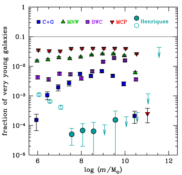
Figure 8: Fraction of very young galaxies (most of the stellar mass formed within the last Gyr) at $z=0$ as a function of galaxy stellar mass for for the analytical galaxy formation models (see Fig. 2) with the bursty galaxy merging scheme. Also shown are the fractions of central galaxies with mean stellar age less than 1 Gyr in the Henriques et al. (2015) semi-analytical model (blue-green circles, filled or empty depending on whether the mass resolution is adequate or not). For the analytical models, which need to be weighted by the halo mass function, the fractions of very young galaxies are taken from equation (23), and the error bars show the uncertainties estimated through 1000 bootstraps (see end of Sect. 4.1). The abscissae are slightly shifted for clarity. The uncertainties for the Henriques semi-analytical model are from binomial statistics, with upper limits indicating 95 percent confidence using Wilson (1927) statistics, see eq. [25]).

In contrast, the Henriques SAM leads to very low fractions (less than 0.03 per cent) of VYGs (defined here as mean mass-weighted age below 1 Gyr) at all masses where it is well resolved ($\log\,(m/{\rm M}_{\odot})\geq 7.5$). The Henriques model thus appears to be discrepant with the 4 analytical models, with 30 to 800 times fewer VYGs predicted by the Henriques SAM at intermediate stellar masses (e.g. $\log m=10^{9}\,{\rm M_{\odot}}$). While these predictions are for the central galaxies in the Henriques SAM, we will see in Sect. 5.1 below that satellites and centrals have similar fractions of VYGs, at these intermediate masses. At masses below $10^{7.5}\,{\rm M_{\odot}}$, the Henriques satellites are typically 5 times less likely to be VYGs than are centrals. However, we do not trust the Henriques results below $10^{7}\,{\rm M_{\odot}}$, because the Henriques SMHM relation, displayed in Fig. 5, shows a suspicious flattening at $\log(m/{\rm M}_{\odot})\approx 6-7$, which appears to be caused by the limited mass resolution of the $N$ body simulation on which the Henriques SAM was run.

4.3 Dependence on critical age

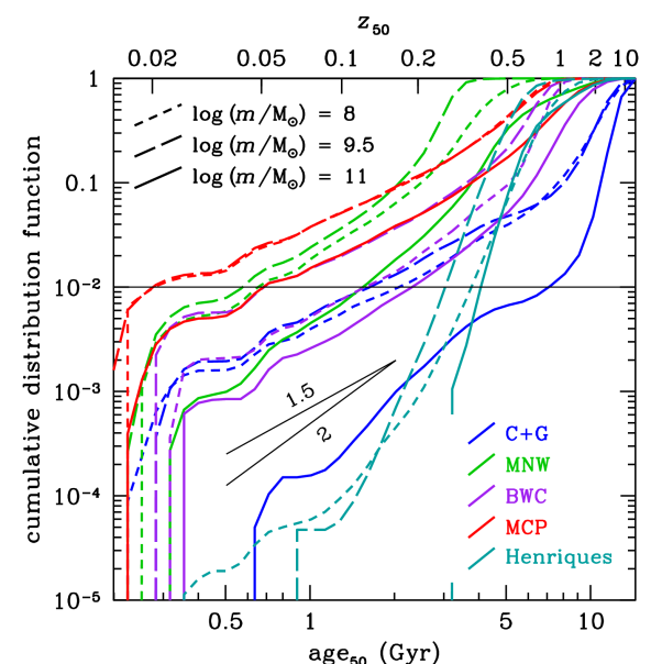
Figure 9: Cumulative distribution functions of galaxy ages for the different models (same colours as in Fig. 6) and for three different bins of stellar mass: $\log(m/{\rm M}_{\odot})=7.25-8.75$ (short dashed), 8.75–10.25 (long-dashed), 10.25-11.75 (solid). The ages are medians (half the mass formed) for the analytical models (with the bursty galaxy merging scheme) and arithmetic means for the Henriques semi-analytical model. The short segments indicate slopes of 1.5 and 2, while the horizontal line indicates the youngest 1 per cent of galaxies.

One may ask how the fraction of VYGs depends on our choice of 1 Gyr for the greatest allowed age for very young galaxies. Figure 9 shows the cumulative distribution function (CDF) of galaxy ages for the different models (using bursty galaxy merging for the analytical ones) in three bins of stellar mass. This allows us to measure how the VYG fraction scales with critical ages not necessarily equal to 1 Gyr. The slopes of the curves near 1 Gyr indicate that the fraction of VYGs roughly scales as $\rm age_{50}^{3/2}$ for most models, but is even more sensitive to the critical age (slope of roughly 2) for models C+G and Henriques at high stellar mass.

Figure 9 also indicates wide variations between the models for the ages of the youngest, say, 1 per cent of galaxies (horizontal line). For the intermediate bin of stellar mass ($\log(m/{\rm M}_{\odot})=9.5\pm 0.75$, long dashed lines), the ages of the 1 per cent youngest galaxies are 0.25, 0.55, 0.65, 1.5, and 3 Gyr for the MCP, MNW, BWC, C+G, and Henriques models, respectively. The discrepancy is as pronounced for the high-mass galaxies ($\log(m/{\rm M}_{\odot})=11.0\pm 0.75$, solid lines): 0.65, 1.5, 2.2, 4, and 7 Gyr, in the same order of models, except that C+G switches with Henriques for the highest age.

4.4 Dependence on the galaxy merging scheme

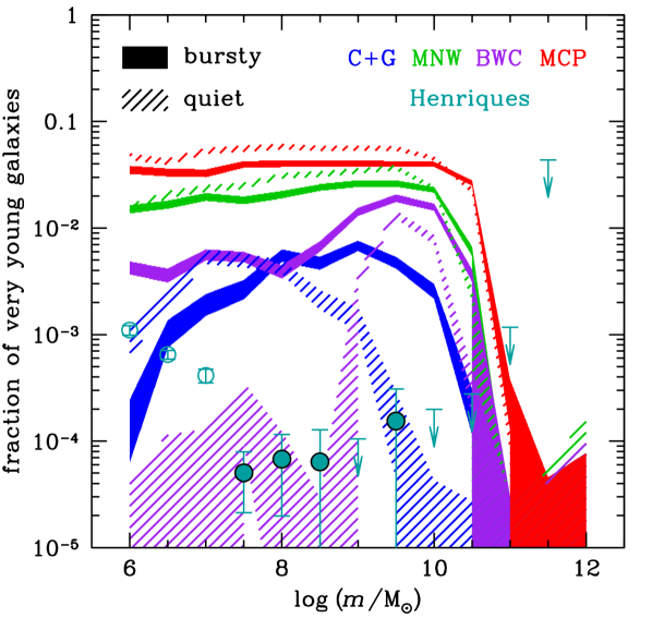
Figure 10: Effect of the galaxy merging scheme used in the analytical models on the fraction of very young galaxies vs. stellar mass. The solid and hatched shaded regions denote the bursty and quiet merging schemes, respectively, where the weights are taken into account according to equation (23), and the errors are based upon 1000 bootstraps. The blue-green points indicate the semi-analytical model Henriques for reference (open circles when the mass resolution is not adequate.

Figure 10 compares the VYG fractions versus mass for the two galaxy merging schemes. It clearly shows the lack of sensitivity of the VYG fractions predicted by the MNW and MCP models to the presence of a burst of star formation associated with the halo merger. However, the merging scheme has an important effect on the C+G and BWC models. For the BWC model, the fraction of VYGs is above 0.1 per cent only in a narrow range of stellar masses around $\log\,(m/{\rm M}_{\odot})=9.5$ for the quiet galaxy merging scheme, with negligible fractions at masses lower than $\log\,(m/{\rm M}_{\odot})=8.5$. For the C+G model, the fraction of VYGs is mostly reduced at intermediate and high stellar masses for the quiet merging scheme. With the quiet merging scheme, only the BWC and C+G analytical models reproduce the very low VYG fractions obtained with the Henriques SAM for stellar masses $7.5\leq\log\,(m/{\rm M}_{\odot})\leq 9$ and $9.5\leq\log\,(m/{\rm M}_{\odot})\leq 10$, respectively, while the other analytical models predict higher VYG fractions in these mass ranges. We will discuss the reasons for these behaviours in Sect. 5.2.

5 Discussion

5.1 Limitations of the galaxy formation models

The galaxy formation models that we considered to assess the frequency of VYGs have several limitations.

The analytical and Henriques SAM were calibrated to observational data in a limited range of redshifts and masses (highlighted in Figures 2 and 4, respectively, for the analytical models). The fractions of VYGs at stellar log masses (in solar units) lower than 8.8 (C+G), 7.4 (MNW and BWC), 10.0 (MCP) are obtained by extrapolating the models. Similarly, the Henriques SAM is calibrated at $z=0$ to $\log\,(m/{\rm M}_{\odot})>7.2$, and at lower stellar mass there is a suspicious flattening of the SMHM in Figure 5, which may be due to insufficient mass resolution.

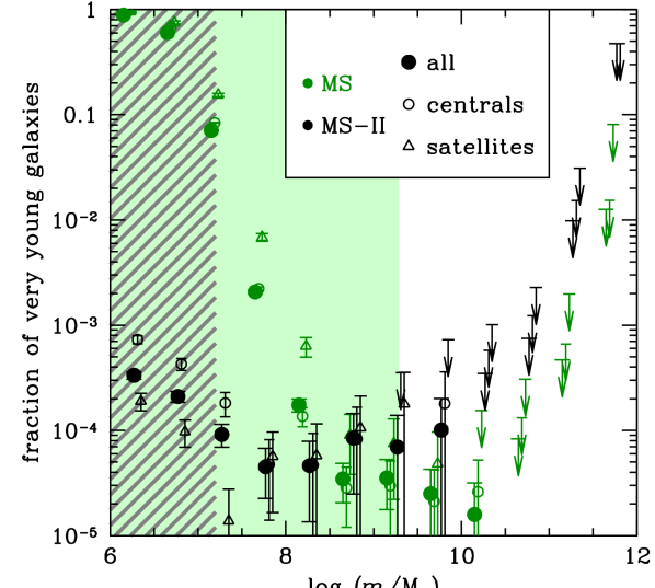
Figure 11: Effect of the mass resolution of the parent dark matter simulation on the fractions of very young galaxies (mean stellar age less than 1 Gyr) obtained with the Henriques et al. (2015) semi-analytical model. The green and black symbols respectively show the results for the Millennium simulation and for the Millennium-II simulation (black), which has 125 times better mass resolution. The light green and hatched grey shaded regions indicate the ranges of stellar masses where the Millennium and Millennium-II simulations are not correctly resolved. The Figure highlights the differences between centrals (open circles), satellites (triangles) and all galaxies (large filled circles). The abscissae are slightly shifted for clarity. The error bars are the uncertainties from binomial statistics (with 95 per cent Wilson upper limits — eq. [25]).

In fact, the mass and spatial resolution of the cosmological simulation on which the Henriques SAM is run has a strong effect on the fraction of VYGs at low galaxy masses. Figure 11 compares the fractions of VYGs versus stellar mass found by the Henriques SAM, when run on the high resolution MS-II simulation and on the 125 times lower mass resolution MS simulation. While the fractions of VYGs are similar at intermediate mass, the MS produces increasingly higher VYG fractions at increasingly lower masses, where it is poorly resolved, than does the MS-II. At $m=10^{7.25}\,{\rm M_{\odot}}$, at the limit where the MS-II is still properly resolved, the Henriques SAM run on the MS leads to VYG fractions up to 3 orders of magnitude higher than found when it is run on the MS-II. The Henriques SAM run on the poor mass resolution MS forms galaxies at later times, which are thus more likely to become VYGs.

The Henriques SAM was run on dark matter simulations that were rescaled in space and time to reproduce the large-scale statistics for a more realistic cosmology (Planck vs. 1st-year WMAP). Tests by Angulo & White (2010) suggest that the small-scale quantities such as halo masses, bulk velocities, and the luminosities of their brightest galaxies are changed by only 10, 5 and 25 per cent, respectively. However, this rescaling may not reproduce the astrophysical processes at small scales, i.e. in the nonlinear regime, in particular the galaxy orbits including dynamical friction, as well as tidal stripping of galaxies by their host groups.

Compared to the Henriques SAM, our 4 analytical models have the advantage of a much superior halo mass resolution: our Monte-Carlo halo merger trees are built for $z$=0 halo masses down to $10^{7}\,{\rm M_{\odot}}$, corresponding to the mass of a single particle in the MS-II simulation on which the Henriques SAM was run. Furthermore, the trees resolve branches down to $10^{3}{\rm M_{\odot}}$. Note that our halo merger trees were only tested by Jiang & van den Bosch (2014) down to $\log(h\,M_{0}/{\rm M_{\odot}})=11$.

On the other hand, our analytical models have also their own drawbacks. The careful reader will have noted that some of the empirical models we use have been calibrated assuming slightly different sets of cosmological parameters (see Table 1). While models MNW and BWC have values of $\Omega_{\rm m}$, $h$ and $\sigma_{8}$ that are within 1 per cent of one another, model MCP has values of $\Omega_{\rm m}$, $h$, and $\sigma_{8}$ that are respectively 8 per cent below, 4 per cent above, and 10 per cent above those from the other two models. Since the VYG fractions of the MNW model are in much better agreement with those of the MCP model than with those of the BWC model (Fig. 8), it appears that the VYG fractions are more sensitive to the baryonic physics than to the details of the cosmological parameters.

Our analytical models do not follow the satellite galaxies that survive by $z=0$ against merging into the central galaxy of their halo. However, Fig. 11 shows that there are no large differences in the VYG fractions of centrals (open circles) versus satellites (triangles) in the Henriques SAM, especially for the SAM run on the higher resolution MS-II, except for $\log(m/{\rm M_{\odot}})\leq 7.5$, where the satellites are typically 5 times less likely to be VYGs.

Moreover, with the bursty galaxy merging scheme applied to our first three analytical models, the stellar mass of the central galaxy is boosted at the time of the halo merger instead of when the satellite mergers into the central, which is at least a third of a current Hubble time Gyr later (see Sect 2.3.7). This boost is the consequence of the larger halo mass of the central galaxy after the halo merger together with the increasing stellar mass of the analytical models with halo mass (given the shallower than –1 slopes in $F_{\rm SFE}$ versus $M$ in the bottom panel of Fig. 2). This will be discussed in detail in Sect 5.2. In the fourth model (MCP), the stellar mass growth is directly linked to the halo mass growth. So, all four models naturally have star formation associated with halo mergers. This should be realistic for haloes that are rich in cold gas and that merge in nearly head-on orbits. If the mergers are off-center, one ought to delay the starburst by the dynamical friction time, and if the mergers are gas-poor, there should be no burst from the halo merger. Since our focus is on low and intermediate mass galaxies, which tend to be gas rich (fig. 11 of Baldry et al., 2008 and references therein), and whose progenitors must have been even more gas-rich, our galaxy merging scheme appears to be sufficiently realistic.

A final worry of the analytical models is that they may not properly consider halo mass accretion histories (MAHs). Indeed, galaxy properties appear to be not only be related to halo mass, but also to halo MAH. In cosmological simulations, the halo MAH influences the clustering of haloes (Gao, Springel & White, 2005) and their concentration (Wechsler et al., 2006), a process known as assembly bias. Such galaxy assembly bias is observed from mass modelling of low redshift galaxies traced by their satellites, which leads to red galaxies (i.e., with older stellar populations) having higher concentration haloes than blue (young stars) galaxies of the same stellar (or halo) mass (Wojtak & Mamon, 2013). Galaxy assembly bias can be detected in the outputs of SAMs (Wang et al., 2013). Our Monte-Carlo halo merger trees incorporate assembly bias to a large extent, since different haloes have different MAHs. But it is not clear that the strong dependence of halo assembly bias with the large scale environment (as predicted by Yang et al., 2017) is implicitly incorporated in our halo merger trees.

5.2 Simple modelling of the fraction of very young galaxies in the analytical models

The relative importance of VYGs in the analytical models can be assessed from first principles. According to our definition, VYGs are produced when the stellar mass, summed over all progenitors, increases by more than a factor of 2 in the last Gyr. This growth in stellar mass occurs in two manners: 1) the quiescent growth from the models in the absence of halo mergers (i.e., at fixed halo mass); 2) the growth by halo mergers and corresponding galaxy mergers. Below, we build a toy model of the stellar mass growth of galaxies that is based on the simplifying assumption that this growth is independent of the past history (in other words our simple model is Markovian).

5.2.1 Model of quiescent growth during last Gyr

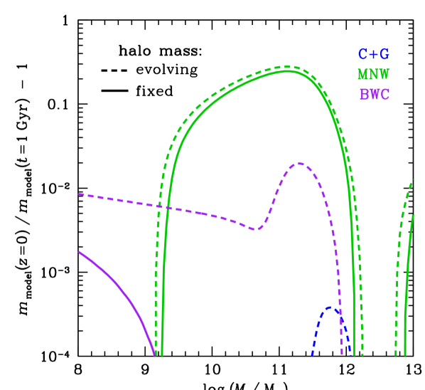
Figure 12: Quiescent growth of stellar mass for the first three analytical models (Cattaneo et al. (2011) with Gnedin (2000) [C+G] (blue), Moster et al. (2013) [MNW] (green), and Behroozi et al. (2013) [BWC] (purple, see Fig. 2) with the bursty galaxy merging scheme. The growth is computed as the time integral of the maximum of the time derivative of the stellar mass and zero (eq. [26]). The solid curves show the quiescent growth with fixed halo mass, while the dashed curves show a hybrid growth, combining the growth of the SFE on top of the median evolution of halo mass. The C+G model shows zero quiescent growth. The time derivatives of the Mutch et al. (2013, MCP, not shown) analytical model are zero at fixed halo mass, hence the model leads to zero quiescent mass growth.

In the absence of mergers, VYGs are produced if the quiescent growth in stellar mass from the analytical model is a factor of 2 since 1 Gyr. The stellar mass will vary during the last Gyr as

$$\Delta m_{\rm quiescent} = m(t_{\rm lookback}=1\,{\rm Gyr})-m(t_{\rm lookback}=0)$$ (26)

$$= \int_{t_{0}-1}^{t_{0}}{\rm Max}\left(0,{{\rm d}m_{\rm model}\over{\rm d}t}\right)\,{\rm d}t\ ,$$

where $t_{0}$ is the age of the Universe expressed in Gyr, $m_{\rm model}(M_{0},z)$ is given in equation (1), and the halo mass is fixed to the $z$=0 value. If the quiescent growth is over 50 per cent, then all galaxies should be VYGs!

The gold band in Figure 3 highlights the quiescent growth of the analytical models during the last Gyr. While model MNW has quiescent growth in the last few Gyr, models C+G and BWC lead to negative growth in the last Gyr. Solving the integral in equation (26), we display in Figure 12 (solid lines) the relative jump in stellar mass during the last Gyr in the absence of halo mergers. Only the MNW model shows significant quiescent growth at some halo masses, with a peak growth of 25 per cent for $\log\,(M/{\rm M}_{\odot})=11.2$ (thick green curves in Figure 12). In comparison, the C+G has no quiescent growth, while that of the BWC model is small for $\log\,(M/{\rm M}_{\odot})<9.4$ and zero at higher halo mass. The MCP model leads to zero stellar mass growth when the halo masses are fixed.

We can also consider the hybrid evolution of stellar mass combining the analytical model $\widetilde{m}(M,z)$ using the median evolution of halo mass instead of fixing the halo mass to its $z$=0 value. Although the median growth of halo mass is small (typically 0.005 dex, increasing with final halo mass), this halo evolution can make a difference in the stellar mass growth. Re-computing the integral of equation (26) assuming the median evolution of halo mass (black curves in Fig. 4, instead of fixed halo mass), we find (dashed curves in Fig. 12) that the relative growth of stellar mass is boosted slightly (to 28 per cent for MNW at $\log\,(M/{\rm M}_{\odot})=11.2$) or strongly (for the C+G and BWC models).

The extremely low quiescent growth of stellar mass in the analytical models implies that mergers are necessary to produce VYGs in these 4 models. But the MNW model at $\log\,(M/{\rm M}_{\odot})=11$ requires less of a boost from mergers than it does at other final halo masses, as well as compared to the other models.

5.2.2 Model of final Gyr stellar mass growth for bursty merging

We next consider the growth of stellar mass, summed over the progenitors, during a halo merger in the case of bursty merging. To keep things simple, we consider (only) two haloes of masses $M_{1}$ and $M_{2}$, with respective stellar masses $m_{1}$ and $m_{2}$, merging at timestep $s$ to reach a new mass of $M=M_{1}+M_{2}$. This simple model does not account for multiple halo mergers in a given timestep.

Considering that the stellar mass of the satellites are frozen, the stellar mass of the pair can be written

$$\Delta m_{\rm pair} \!\!\!\!=\!\!\!\! {\rm Max}\left[\widetilde{m}(M_{1}\!+\!M_{2},s),\widetilde{m}(M_{1},s\!-\!1)\right]-\widetilde{m}\left(M_{1},s\!-\!1\right)$$ (27)

$$\!\!\!\!=\!\!\!\! {\rm Max}\left[\widetilde{m}(M_{1}\!+\!M_{2},s)\!-\!\widetilde{m}(M_{1},s\!-\!1),0\right]\,.$$

Since the dynamical friction time (eq. [19]) is always greater than 6.7 Gyr for lookback times less than 1 Gyr (Sect. 2.3.7), the satellites that were involved in halo mergers in the last Gyr do not have time to merge with the main galaxy.

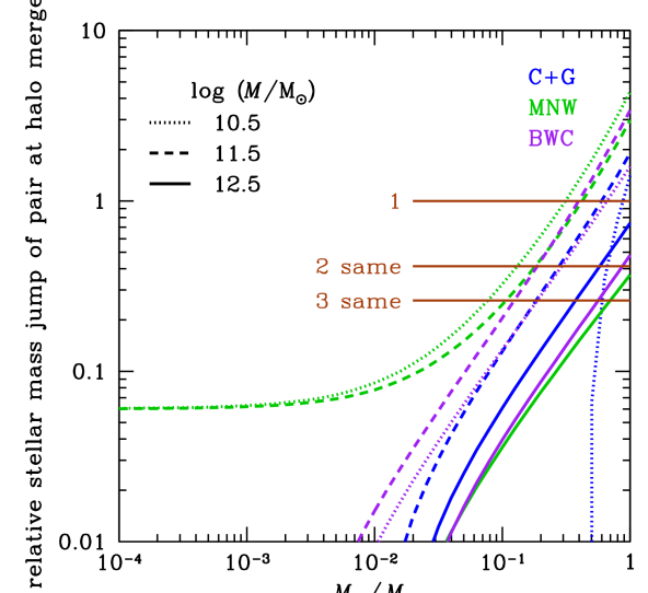
Figure 13: Relative growth of stellar mass of merging pair (mass ratio minus unity) at the time of the halo merger predicted from our simple model (eq. [27]) versus the halo mass ratio (above $10^{-4}$ in our Monte Carlo simulations), for the three analytical models shown in Figure 12, with the bursty galaxy merging scheme, for three masses of the merged halo. The halo merger is assumed to occur at $z=0.04$ (lookback time of 520 Myr). For the C+G model, we used equation (28) to correct the model stellar mass at $\log\,(M/{\rm M}_{\odot})\leq 11.2$ in equation (27) to conform with the mass found in Fig. 5. The brown horizontal lines indicate jumps in stellar mass that would double it in a single merger, or in 2 or 3 mergers of same halo mass ratios.

Figure 13 shows how the stellar mass of the merging pair evolves from the previous timestep to the halo merger one using equation (27), for the C+G, MNW, and BWC models. Since we do not follow satellites, we thus normalize the jump in stellar mass by the stellar mass $m_{1}$ of the first galaxy. While the $z$=0 SMHM matches quasi-perfectly the model prediction for the MNW and BWC models, it predicts less stellar mass for the C+G model at $\log\,(M/{\rm M}_{\odot})\leq 11.2$ (Fig. 5), because the stellar mass is frozen when $F_{\rm SFE}$ reaches its maximum over 8 Gyr ago (Fig. 3). The excess log stellar mass in the C+G model is well fit (to 0.06 dex rms accuracy) by

$$\Delta\log\left({m\over{\rm M_{\odot}}}\right) \!\!\!\!=\!\!\!\! 1.100-1.678\,\log\left({M\over 10^{10}\,{\rm M_{\odot}}}\right)$$ (28)

$$\qquad\quad+0.633\,\log\left({M\over 10^{10}\,{\rm M_{\odot}}}\right)^{2}\ .$$

We thus correct our C+G model stellar mass using equation (28).

Given that 1 Gyr corresponds to 3 timesteps, the galaxy has three chances to boost its stellar mass by a factor 2 by mergers. The brown horizontal lines in Figure 13 indicate relative stellar mass jumps amounting to a doubling of stellar mass in a single halo merger or in 2 or 3 mergers of equal halo mass ratio. The intersection of the curves with these lines provides the minimum halo mass ratio of a single merger, or 2 or 3 halo mergers of the same mass ratio, to allow this doubling of stellar mass. Three halo masses are shown that, through the SMHM relation of Fig. 5 correspond to stellar masses in the rough range $7.5\mathrel{\hbox{\hbox to0.0pt{\hbox{\lower 4.0pt\hbox{$\sim$}}\hss}\hbox{$<$}}}\log\,(m/{\rm M}_{\odot})\mathrel{\hbox{\hbox to0.0pt{\hbox{\lower 4.0pt\hbox{$\sim$}}\hss}\hbox{$<$}}}10.6$ (depending on the model).

For the C+G and BWC models, the jumps in halo mass for $\log\,(M/{\rm M}_{\odot})=10.5$ (dotted curves in Fig. 13) are too small to reach the minimum necessary boost from 2 identical mergers, even for 1:1 mass ratios. This means that it is virtually impossible to double the stellar mass in the last Gyr for these halo masses. For the MNW model, the plateau of the relative stellar mass jump at low halo mass ratio, for low and intermediate halo masses, suggests that this model may be able to produce low and intermediate stellar mass VYGs through minor halo mergers.

The expected numbers of halo mergers per 350 Myr timestep can be obtained from theoretical analyses (Neistein & Dekel, 2008) or from the analysis of cosmological simulations (Fakhouri, Ma & Boylan-Kolchin, 2010), both of which are very similar. We adopt the differential halo merger rate per unit redshift of Fakhouri et al.

$${\cal R}(M,\mu,z) \!\!\!\!\equiv\!\!\!\! {{\rm d}^{2}N_{\rm merge}\over{\rm d}\mu\,{\rm d}z}$$ (29)

$$\!\!\!\!=\!\!\!\! A\left({M\over M_{\rm ref}}\right)^{b}\mu^{c}\,\exp\left[\left({\mu\over\mu_{\rm ref}}\right)^{d}\right]\,(1\!+\!z)^{e}\ ,$$

where $\mu=M_{2}/M_{1}$ is the halo mass ratio (with $M_{1}+M_{2}=M$) and where $A=0.010$, $M_{\rm ref}=10^{12}\,{\rm M_{\odot}}$, $b=0.133$, $c=-1.995$, $\mu_{\rm ref}=0.00972$, $d=0.263$, and $e=0.010$. Integrating over halo mass ratios, we first infer that in the 350 Myr timestep, a halo of mass $M=10^{10}$, $10^{11}$, or $10^{12}\,{\rm M_{\odot}}$ is expected to be involved in respectively $\langle N_{\rm m}\rangle=2$, 3, or 4 mergers with halos of mass ranging from $10^{-4}\,M$ (the extreme mass ratio allowed in our Monte-Carlo halo merger tree, see Table 1) to $M$. Hence, halo mergers are ubiquitous in our halo merger tree, although there are non-negligible probabilities ($100\,\exp(\langle-N_{\rm m}\rangle)=14$, 5, and 2 per cent respectively for $\log\,(M/{\rm M}_{\odot})=10$, 11, and 12) that a halo suffers no merger in a given timestep. We note here that according to the tests of Jiang & van den Bosch (2014), the Parkinson et al. (2008) code reproduces the halo merger rates of Fakhouri et al. to better than 20 per cent for all mass ratios for low- and intermediate-mass haloes ($M=10^{11}\,h^{-1}\,{\rm M_{\odot}}$ and $10^{13}\,h^{-1},{\rm M_{\odot}}$ at $z=0$).

We can go one step further and integrate the halo merger rate. Let $g_{\rm q}(M)$ and $g_{\rm m}(M,\mu)$ respectively be the quiescent relative growth over 1 Gyr and the relative growth through a halo merger. The predicted fractions of VYGs obtained in two mergers can then be written (dropping the dependence of halo mass and redshift in the expression for the halo merger rate ${\cal R}$ for clarity)

$$f_{\rm VYG}=\left({0.08\over 3}\right)^{2}\,\int_{0.0001}^{1}{\cal R}(\mu_{1})\,{\rm d}\mu_{1}\,\int_{\mu_{2}^{\rm min}}^{1}{\cal R}(\mu_{2})\,{\rm d}\mu_{2}\ ,$$ (30)

where the factor in front of the integral in equation (30) is for the conversion from $\Delta z=1$ to one-third of a Gyr, while the lower limit of the first integral is the resolution of the Monte-Carlo halo merger tree that we have used (Table 1). In equation (30), $\mu_{2}^{\rm min}$ is the solution of the equation

$$(1+\eta\,g_{\rm q})\,\left\{1+g_{\rm m}\left[\left({M\over 1+\mu_{2}}\right),\mu_{1}\right]\right\}\,\left[1+g_{\rm m}(M,\mu_{2})\right]=2\ ,$$ (31)

for $\mu_{2}$, with $\eta=1/3$ to account for the fact that only one-third of the Gyr interval is available for quiescent growth (since we do not bother to perform the triple integral required for the three timesteps).

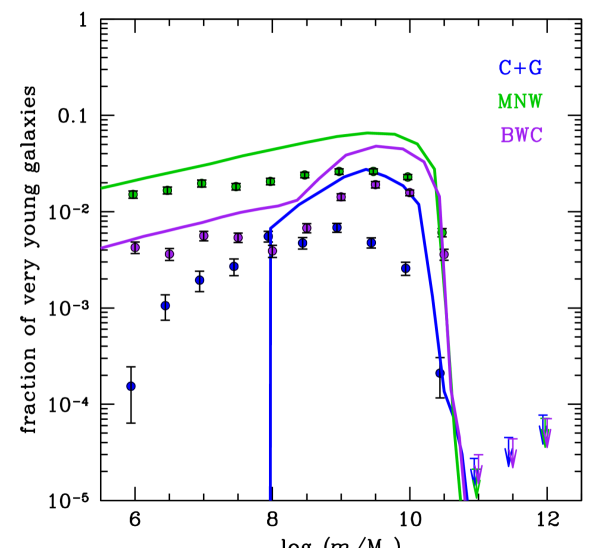
Figure 14: Predicted fractions of very young galaxies for the first three analytical models (with the bursty galaxy merging scheme) as a function of $z$=0 stellar mass, from our simple Markovian model (curves) combining quiescent growth and growth during halo mergers (eqs. [26–30]), compared to those from the Monte Carlo halo merger trees (symbols as in Fig. 8), where the abscissae are slightly shifted for clarity.

The curves in Figure 14 show the fractions of VYGs predicted by our simple model (which involves no Monte-Carlo halo merger trees), as given by equation (30). The figure captures the basic features of VYG fractions we found with the analytical models applied to the Monte-Carlo halo merger trees (Fig. 8 and shown as symbols in Fig. 14). In particular, the MNW and BWC models are both remarkably well reproduced: the MNW model shows a few per cent VYGs at low and intermediate stellar masses and a sharp drop at higher masses (with the simple model overpredicting the Monte Carlo halo merger tree calculations by a factor of 2). Similarly, our simple model catches the details of the BWC model. However, our model is less successful in predicting the VYG fractions with the C+G model, as it misses the 0.001 fraction of VYGs at $\log\,(m/{\rm M}_{\odot})<8$. (Had we not corrected for the excess stellar mass of the C+G model galaxies compared to their model predictions, eq. [28], the predicted C+G VYG fraction would be a factor 3 above that of the MNW model at low mass.) These discrepancies may be attributable to the simplicity of our model and to the large scatter in the SMHM of the C+G model at low mass. Nevertheless, the agreement for the MNW and BWC models of our simple VYG model with the VYG fraction measured by the full model on the Monte-Carlo halo merger trees suggests that the galaxy histories before 1 Gyr matter little in predicting the MNW and BWC VYG fractions, while the C+G VYG fractions, on the contrary, appear to depend on past history.

5.2.3 Model of final Gyr stellar mass growth for quiet merging

For the quiet merging scheme, we can better understand the jump in stellar mass with a toy model based on equation (18).

Consider a halo of mass $M_{0}$ at lookback time $t=t_{0}$ (corresponding to $z=0$) and assume that its stellar mass $m_{0}$ is given by its model stellar mass $\widetilde{m}_{0}=\widetilde{m}(M,0)$. This corresponds to the first term within the brackets of equation (18) dominating the second one. Let ${\cal F}_{i}(M)$ be the fraction of halo mass $M$ at lookback time $t_{i}$ (corresponding to redshift $z_{i}$) that came from branches that merged at lookback time $\geq t_{i}$ and whose host satellites are not expected to merge (after dynamical friction) before lookback time $t$. In other words, ${\cal F}$ measures the fraction of halo mass coming from branches with surviving satellites. The stellar mass at $z=0$ can then be written

$$m_{0}\equiv\widetilde{m}_{0}=\widetilde{m}\left(\left[1\!-\!{\cal F}_{0}(M_{0})\right]M_{0},0\right)\ .$$ (32)

At lookback time $t_{1}=1\,\rm Gyr$, corresponding to redshift $z_{1}$, we write the stellar mass summed over the progenitors of the $z=0$ galaxy as

$$m_{1}=\widetilde{m}\left(\left[1\!-\!{\cal F}_{1}(M_{1})\right]M_{1},z_{1}\right)+\sum m_{\rm sats}\ ,$$ (33)

where $M_{1}$ is the mass of its main progenitor at lookback time $t_{1}$. The last term in equation (33) is the total stellar mass in satellites that merge with the central between lookback times $t_{1}$ and 0 (recall that the stellar masses of satellites are frozen).

Let $\overline{\cal F}_{i}(M)$ be the median value expected for the values of ${\cal F}_{i}(M)$ and $\eta_{i}(M)={\cal F}_{i}(M)/\overline{\cal F}_{i}(M)$, for $i=1$ and 0. Thus, $\eta_{i}(M)$ represents the excess, relative to the median, of the mass fraction of halo of mass $M$ at lookback time $t_{i}$ that originates from branches whose galaxies would survive as satellites until a lookback time $t<t_{i}$. A halo with $\eta>1$ is one that could be considered fortunate to have a higher fraction of its mass than usual from branches with surviving satellites.

The condition for obtaining a VYG is $m_{0}>2\,m_{1}$ using equations (32) and (33). Solving this inequality is difficult, because of the range of redshifts when haloes merged with the main progenitor of the current halo, yet their satellites survived. So, for simplicity, we assume that the satellite term in equation (33) contributes to a fraction $f_{\rm sats}$ of the mass $m_{1}$. Moreover, we adopt for $M_{1}$ the median mass $\overline{M}_{1}$ expected for the $z$=0 halo mass $M_{0}$. The black curves of Figure 4 indicate a very slow typical growth of the main halo progenitor in the last Gyr, of order of 0.005 dex (Sect. 5.2.1). We shall see (Sect. 5.4 below) that contrary to the case of bursty galaxy merging, VYGs are not related to rapid jumps in halo mass with the quiet merging scheme. With these assumptions and equations (32) and (33), the condition for a VYG is

$$\left.\begin{aligned} &\widetilde{m}\left(\left[1-\eta_{0}(M_{0})\,\overline{\cal F}_{0}\left(M_{0}\right)\right]M_{0},0\right)\\ &\quad>{2\over 1-f_{\rm sats}}\,\widetilde{m}\left(\left[1-\eta_{1}(\overline{M}_{1})\,\overline{\cal F}_{1}\left(\overline{M}_{1}\right)\right]\overline{M}_{1},z_{1}\right)\ .\end{aligned}\right.$$ (34)

Of course, since VYGs are predicted to be rare at all masses, typical values of ${\cal F}(M)$ (i.e. $\eta_{0}=\eta_{1}=1$) will not lead to VYGs according to equation (34). Instead, the requirement for obtaining a VYG is to have $\eta_{0}<1$ and/or $\eta_{1}>1$, i.e. a final halo with a low mass fraction from branches with surviving satellites and/or progenitors at 1 Gyr lookback time with high mass fraction from branches with surviving satellites (to 1 Gyr lookback time). Here, we assume $\eta_{1}=1$ and determine the maximum value $\eta_{0}^{\rm VYG}$ of $\eta_{0}$ for obtaining a VYG. If $\eta_{0}^{\rm VYG}$ is only slightly below unity, VYGs will be easier to form than if it is much lower than unity.

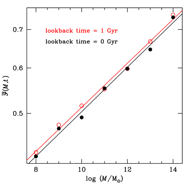
Figure 15: Median fraction of halo mass from branches hosting surviving satellites (from eq. [35]), as function of halo mass for two lookback times. The lines are linear fits of $\log\overline{\cal F}$ vs log halo mass.

The median value $\overline{\cal F}(M)$ is not straightforward to extract, e.g. from extended Press Schechter theory (e.g., Neistein & Dekel, 2008; Parkinson et al., 2008).

Instead, we estimate $\overline{\cal F}(M)$ by considering the median halo growth:

$${\cal F}_{i}(M)={1\over M}\,\sum_{\begin{subarray}{c}t^{\prime}>t_{i}\\ \tau_{\rm df}>t^{\prime}-t_{i}\end{subarray}}\left[\overline{M}(t^{\prime}\!-\!\Delta t_{i})-\overline{M}(t^{\prime})\right]\ ,$$ (35)

where $\overline{M}(t^{\prime})$ is the median mass expected for a halo at lookback time $t^{\prime}$, whose mass at lookback time $t_{i}$ is $M$, $\Delta t$ is the previous timestep, and where the dynamical friction time is $\tau_{\rm df}\equiv\tau_{\rm df}\left[\overline{M}(t^{\prime}),\overline{M}(t^{\prime}-\Delta t)-\overline{M}(t^{\prime}),t^{\prime}\right]$. The expression for ${\cal F}$ given in equation (35) corresponds to summing up all the masses of secondary progenitors merging with the primary ones. It is an underestimate, because it assumes that halo merging is binary. If, instead, many branches merge at once, each branch will correspond to a lower mass progenitor and its dynamical friction time would be longer. We thus assume that the lower mass branches bring negligible mass to the final halo.

Figure 15 shows that $\overline{\cal F}(M)$ is of order one-half, weakly increasing with halo mass, and with very little dependence on the final considered lookback time. The linear fit in log-log space yields

$$\log\overline{\cal F}(M)\simeq a+b\,\log\left({M\over{\rm M_{\odot}}}\right)\ ,$$

with $a=-0.686$ and $b=0.0389$ for $z=0$, and $a=-0.674$ and $b=0.0383$ for lookback time of 1 Gyr. This median surviving fraction $\overline{\cal F}(M)$ increases with halo mass, because large halo masses grow faster, hence the values of $M_{2}$ are relatively more important (this offsets the shorter dynamical friction times, since they are always greater than one-third of the current Hubble time).

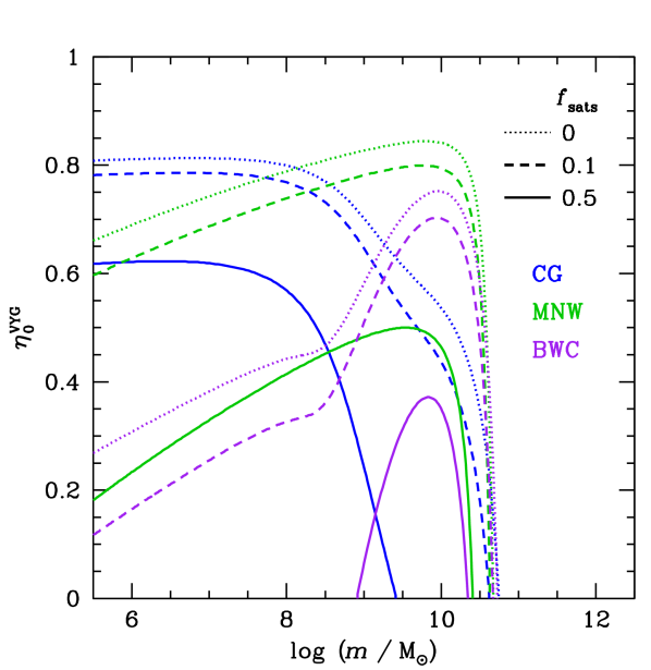
Figure 16: Maximum excess fraction $\eta_{0}^{\rm VYG}$ of final halo mass coming from branches that merged recently enough that the galaxies survive as satellites at $z=0$ to yield very young galaxies versus final stellar mass. The parameter $\eta_{0}^{\rm VYG}$ is derived by solving equation (34), using Fig. 15 for $\overline{\cal F}(M)$, assuming $\eta_{1}=1$ and the $z$=0 stellar - halo mass relation predicted by the model. The dotted, dashed, and solid curves display the results when assuming that $f_{\rm sats}=0$, 0.1, and 0.5, respectively.

We can combine equations (34) and (35) to estimate the maximum value of $\eta_{0}^{\rm VYG}$ to obtain VYGs. Figure 16 shows the maximum values of $\eta_{0}$ to obtain a VYG, for the C+G, MNW, and BWC models. We assumed $\eta_{1}=1$ and converted the final halo masses to stellar masses using the SMHM predicted by the model. Figure 16 can be compared to the hatched shaded regions of Figure 10, corresponding to the VYG fractions obtained with the quiet merging scheme applied to the Monte Carlo halo merger tree. For all choices of $f_{\rm sats}$, we recover the sharp drop of VYG fractions at $\log\,(m/{\rm M}_{\odot})\simeq 10.7$ for all 3 models. We also recover most of the hierarchy between the 3 galaxy formation models: C+G should produce a much higher fraction of VYGs than BWC at low mass, BWC should overtake C+G at intermediate mass, and the MNW model should dominate the others at intermediate masses. The only weakness of our simple model is that it fails to recover the higher fraction of VYGs expected with the MNW model at low masses in comparison to the C+G model. This might be explained by a higher value of $f_{\rm sats}$ for the C+G model, whose quiescent evolution is frozen earlier than the other models by our prevention of decreasing stellar masses, as seen in Figure 3.

5.3 Evolutionary histories

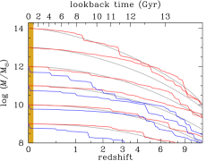
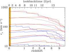
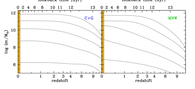
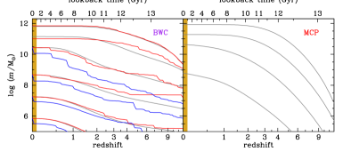
Figure 17: Evolutionary histories of haloes and galaxies for haloes with final log masses from 9 to 14 in steps of 1 (going upwards). Top: Evolution of the main progenitor of the $z$=0 haloes in mass (top left) and circular velocity (top right). Middle & bottom: Evolution of the total stellar mass (summed over all progenitors) of galaxies for the four models with bursty galaxy merging, with the same $z$=0 halo log masses. The smooth grey curves represent the median evolutionary histories. For the BWC model, the broken curves represent particular histories of galaxies, which at $z=0$ are very young (blue) or normal (red). The evolution of the corresponding haloes are displayed in the same colours (top panels). Note the different cosmologies used for each model to link lookback time and redshift.

Figure 17 shows (grey curves) the median evolution of the main halo progenitor in mass and circular velocity (top panels) and the median evolution of the stellar mass, summed over all progenitors, for the 4 analytical models. One notices that for intermediate halo masses ($\log\,(M/{\rm M}_{\odot})=13$), the median evolution of haloes since $z=1$ is at constant circular velocity (see Mamon et al., 2012), while at low masses halo mass growth is so weak that halo mass is nearly constant.

As seen in the lower 4 panels of Fig. 17, the median stellar mass evolution (whose time derivative corresponds to the star formation rate) can be growing or nearly frozen depending on the analytical model and the final halo mass.

The bottom left panel of Figure 17 displays the evolution of stellar mass for representative very young (blue) and old (red) galaxies for the BWC model with delayed galaxy merging (which produces no VYGs for massive haloes, $\log\,(M/{\rm M}_{\odot})\geq 13$). The VYGs can be easily spotted by a sharp growth in the stellar mass at low redshift, and are caused by the rapid halo mass growth (top left panel). The bottom left panel of Figure 17 shows examples of VYGs produced with unusual long-term histories (the example ending at $\log\,(m/{\rm M}_{\odot})=10.5$) and others with very typical histories (the examples ending at $\log\,(m/{\rm M}_{\odot})=8.7$, 7.3, and 5.9). This illustrates the Markovian nature of the BWC model (Sect. 5.2): the production of VYGs is not determined by the long-term histories of the galaxies.

5.4 Statistics of halo growth in last Gyr

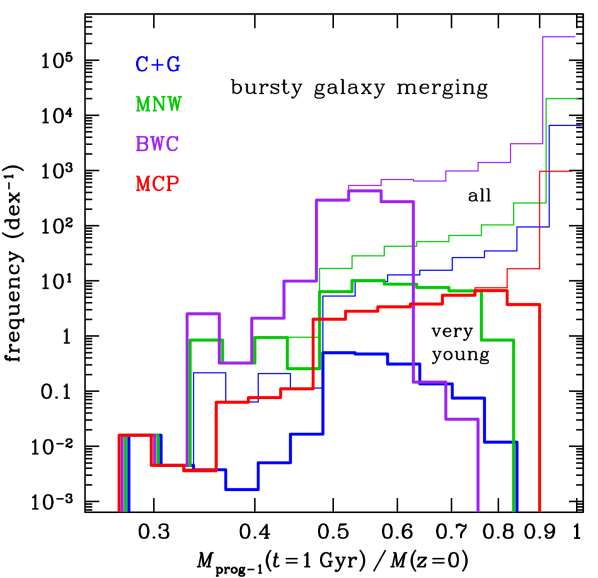
Figure 18: Frequencies of the inverse growth of the most massive halo progenitor in the last Gyr, for all (thin) and very young (thick histograms) galaxies, for the 4 analytical models (see Fig. 2) for bursty galaxy merging. The abscissae above 3/4 indicate no mergers with mass ratios between 1:1 and 3:1, while those below 1/2 indicate more halo growth than a single 1:1 major merger. The frequencies of halo mass ratios are weighted according to equation (21).

One may ask whether, in the analytical models, the final rapid growth of stellar mass (summed over all progenitors) is indeed linked with a corresponding rapid growth in the most massive progenitor of a galaxy’s halo. Figure 18 shows the statistics of halo mass growth in the last Gyr. The abscissae (slightly shifted for clarity) above 3/4 indicate no mergers with mass ratios between 1:1 and 3:1, while those below 1/2 indicate more halo growth than a single 1:1 major merger. In the C+G and BWC models, the rapid recent growth in total stellar mass for the VYGs indeed comes hand-in-hand with rapid mass growth of the most massive progenitor of the halo. In contrast, the MNW and, especially, MCP models show fairly frequent cases of rapid final growth in stellar mass that occurs with slow halo mass growth. To summarize, the median halo relative mass growth from 1 Gyr to the present is of order 0.015 for all galaxies, but for VYGs it is as high as 0.4 (MCP), 0.6 (MNW), 0.8 (BWC), and 0.9 (C+G). This suggests the important role of major halo mergers. However, in nearly one-quarter of the VYGs in the MCP model, the haloes grow by less than 25 per cent, indicating that more minor halo mergers suffice.

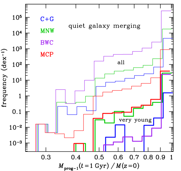
Figure 19: Same as Fig. 18, but for the quiet galaxy merging scheme.

Figure 19 shows a very different halo merging history for the VYGs obtained with quiet galaxy merging: most of the VYGs are associated with haloes that only slowly increase their mass in the last Gyr. The distribution of the values of halo mass growth in the last Gyr are indistinguishable between the VYGs and all galaxies. This is the consequence of the stellar mass no longer being a function of the current halo mass, but instead of the current halo mass minus the mass in the subhaloes that host surviving satellites (eq. [18]).

5.5 The effect of the galaxy environment

Our analytical models completely miss the effects of a galaxy’s environment. Analyses of large observational samples of galaxies by Weinmann et al. (2006) and von der Linden et al. (2010) indicate that the fraction of star forming galaxies is reduced in both massive global environments (high-mass clusters) and in the inner local environments (the inner regions of groups and clusters). Since most galaxies belong to groups or clusters (e.g., Yang et al., 2007), one may expect that the lack of environmental effects in our analytical models may cause substantial modifications to the fraction of VYGs.

The abundance matching analytical models mix the different environments to yield a global SMHM relation. However, moving from high to low-mass groups, their central galaxies become increasingly likely to be of spiral morphology (Weinmann et al., 2006) and with efficient star formation (Woo et al., 2013). One needs to go beyond standard abundance matching and also incorporate the link between stellar ages and halo formation times (as indirectly observed by Wojtak & Mamon, 2013, see Sect. 5.1, above), as this allows reproducing correctly several environmental trends (Hearin & Watson, 2013), in particular the fraction of star forming central galaxies as a function of their luminosity (which is known to correlate strongly with stellar and group mass).

Therefore, the quenching of star formation by the environment may explain why the Henriques SAM leads to typically 100 times lower fractions of VYGs at intermediate mass ($8\leq\log\,(m/{\rm M}_{\odot})\leq 10$) in comparison with the analytical models with bursty galaxy merging. However, one cannot unreservedly believe the results of the Henriques SAM, because of its limited mass resolution and also because the treatment of the physics of quenching in SAMs is still very approximate. Moreover, Figure 7 indicates that the typical ages of galaxies in the Henriques SAM are of the same order as those found by MNW, BWC, and MCP models, but their spread is very narrow at intermediate stellar mass, leading to much lower VYG fractions in this mass range.

5.6 Effects of the primordial density fluctuation spectrum

Recently, there has been much interest in allowing for a warmer primordial density fluctuation spectrum than allows the $\Lambda$CDM model. Moving from $\Lambda$CDM to $\Lambda$WDM means that high wavenumber primordial density fluctuations are suppressed. This decreases (but does not suppress) the variance of low-mass fluctuations, making them rarer at given epochs. This in turn means that haloes of given $z$=0 mass collapse later. This effectively reduces the numbers of low-mass haloes at all epochs, potentially solving (Bode, Ostriker & Turok, 2001; Avila-Reese et al., 2001) the problem of the overabundance of such low mass haloes in cosmological $N$-body simulations (Moore et al., 1999). Since present-day stellar mass varies monotonically with halo mass, one concludes that low-mass galaxy formation is delayed in the $\Lambda$WDM model. Therefore, the fraction of VYGs should be enhanced in the $\Lambda$WDM cosmology.

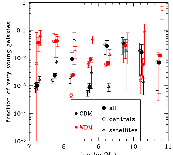
Figure 20: Effect of the primordial density fluctuation spectrum on the fractions of very young galaxies (half the stellar mass formed in the last 1 Gyr), for the Menci et al. (2014) semi-analytical model, run on Monte-Carlo halo merger trees based on two cosmologies: Cold Dark Matter (black) and Warm Dark Matter (with particle mass $m_{\chi}=0.75\,\rm keV$, red). The figure highlights the differences between centrals (open circles), satellites (triangles) and all galaxies (large filled circles). The abscissae are slightly shifted for clarity. The error bars are the uncertainties estimated from 1000 bootstraps.

We have extracted the fractions of VYGs from the Menci et al. (2014) SAM (first presented in Menci et al., 2008, see Sect. 2.4.2), run on two forests of Monte-Carlo halo merger trees, one for $\Lambda$CDM, the other for $\Lambda$WDM. The Menci et al. SAM was run with the exact same parameters on both forests. Figure 20 shows that, for the CDM model, the fraction of VYGs among intermediate mass galaxies is typically 50 times greater than predicted by the Henriques SAM run on the high-resolution MS-II simulation. The VYG fraction among low-mass satellites is significantly greater in the Menci et al. SAM (run on both CDM and WDM halo merger trees) than among centrals in the same mass range, which is opposite to the trend found in the Henriques SAM (Fig. 11).

Figure 20 also illustrates the effects of the primordial density fluctuation spectrum on the fractions of VYGs. We see that the power spectrum has little effect on the fraction of VYGs at intermediate masses, while the passage from CDM to WDM boosts the fraction of VYGs among high-mass satellites. On the other hand, moving from CDM to WDM leads to 10 to 30 times more VYGs at low masses ($m<10^{9}\,{\rm M_{\odot}}$, except for one of the four mass bins – at $\log\,(m/{\rm M}_{\odot})=8.25$), both for centrals and satellites, although this increase is not statistically significant for the centrals (except in the bin at $\log\,(m/{\rm M}_{\odot})=8.75$). This basically confirms the basic trend for younger galaxies with $\Lambda$WDM found by Calura et al. (2014) for this SAM. The boost in the fraction of VYGs among low-mass galaxies but not higher mass ones is an illustration of the WDM power spectrum that suppresses high wavenumbers. Star formation in low-mass galaxies is thus delayed, making a higher fraction of low-mass galaxies appear very young at $z=0$. With the WDM particle mass of 0.75 keV, the boost in the VYG fraction occurs at masses $m<10^{8}\,{\rm M_{\odot}}$. Had we considered a higher WDM particle mass, the boost in the VYG fraction would have occurred at even lower galaxy mass.

These conclusions must be somewhat tempered by the fact that the Menci Monte Carlo halo merger trees are not well resolved at low masses. At stellar masses $\log\,(m/{\rm M}_{\odot})=7\pm 0.25$ and $8\pm 0.25$, the corresponding halo masses have a median of $\log\,(M/{\rm M}_{\odot})=9.5$ and 10, respectively (see also the bottom panel of Fig. 5), so given the minimum branch mass of $\log\,(M/{\rm M}_{\odot})=7.7$ (Table 1), the mass resolution of the trees is only respectively 60 and 200, compared to $10^{4}$ for our four analytical models.

Note also that the Menci et al. (2014) SAM, based upon Monte-Carlo halo merger trees, includes a rough treatment of the environmental effects on galaxies. It leads to intermediate fractions of VYGs at intermediate mass (i.e. for their CDM run) in comparison with the high VYG fractions of the analytical models and the low VYG fractions of the Henriques SAM (compare Figs. 8 and 20).

6 Conclusions

6.1 Method and models

In this work, we modelled the frequency of VYGs (defined to be those with over half the stellar mass having formed within the last 1 Gyr, corresponding to $z=0.08$), among central galaxies, as a function of present-day stellar mass. For this, we first produced over a quarter million Monte-Carlo halo merger trees derived from the code of Parkinson et al. (2008). We then ran four simple models of galaxy formation on these halo merger trees. The first three models give the galaxy stellar mass as a function of halo mass and redshift. These are the physically-motivated model (Cattaneo et al., 2011 with the refined reionization feedback of Gnedin, 2000), and the empirical models of Moster et al. (2013) and Behroozi et al. (2013) obtained by abundance matching of the halo mass function with the observed SMF (with, for the latter, additional constraints on the cosmic star formation rate and the specific star formation rate as a function of mass). We also considered a fourth analytical model by Mutch et al. (2013), where the stellar mass growth rate is proportional to halo mass growth rate and a simple function of halo mass and redshift.

These analytical models present differences in the star formation efficiency as a function of halo mass and redshift (Figs. 2 and 4), because i) one (C+G) is physically motivated while the other 3 are empirical; ii) only one (BWC) is calibrated to data extending to the epoch of reionization; iii) only one (MCP) is based on mass growth rates instead of masses. We also considered two SAMs, which incorporate much more complex physics: one (Henriques) with the advantage of being based on realistic galaxy positions (based on subhaloes from a dark matter cosmological simulation), the other (Menci) that was run on both CDM and WDM cosmologies. Our analytical models run on Monte-Carlo halo merger trees have the advantage of having more statistics at the high halo mass end and higher mass resolution.

We updated the stellar masses of our analytical models using two galaxy merging schemes, one involving a starburst at the time of the halo merger, and one without it. These two schemes should bracket the evolution of stellar masses.

The galaxy formation models applied to the halo merger trees produce somewhat different halo to stellar mass relations (Fig. 5). Yet, they generally match well (especially the MNW and BWC models) the analytical stellar to halo mass relations that they predict at the redshift where half the mass in stars is formed. These models predict stellar mass functions that generally agree with the observations, but with noticeable differences in the low-end slopes.

The dependence on stellar mass of the epoch when half the final stellar mass is formed (measuring the stellar mass evolution by considering all the progenitors, not just the main one) shows differences between the galaxy formation models ran with the bursty merging scheme. All four analytical models and the SAM show downsizing at the high mass end: the median stellar ages decrease with decreasing stellar masses, reaching a minimum around $\log(m/{\rm M_{\odot}})\simeq 9.5$ (see Fig. 7). The C+G model shows strong upsizing (stellar age increasing with decreasing stellar mass) at the low end, while the MNW, BWC, and Henriques models show weak upsizing. The typical median ages at $m=10^{8-10}\,{\rm M_{\odot}}$ range from 2.5 to 11 Gyr (Fig. 7), according to the model. These differences between models can be explained by differences in their star formation efficiencies as a function of halo mass and redshift (Fig. 4) combined with our preventing stellar masses to decrease in time.

6.2 Frequency of very young galaxies

At $z=0$, the fractions of galaxies that are very young depend on the galaxy stellar mass, as well as on the model and the scheme for galaxy mergers. For bursty galaxy merging, the predicted fraction of VYGs is roughly flat up to $10^{10}\,{\rm M_{\odot}}$ for the analytical models, with peaks at typically a few percent at stellar mass near $10^{9}\,{\rm M_{\odot}}$ (Fig. 8). For quiet galaxy merging, the VYG fractions are similar to those with bursty merging for two models (MNW and MCP), but suppressed for two others, at respectively intermediate (C+G) and low (BWC) stellar masses.

With bursty galaxy merging, VYGs are always (C+G and BWC) or often (MNW and MCP) associated with rapid late halo growth (Fig. 18), indicating that most VYGs are associated with recent major halo mergers. However, the MNW, and especially MCP models also allow for stellar mass buildup with halo mergers of intermediate mass ratios (Fig. 18). With quiet galaxy merging, we found, instead, no relation between halo mass growth and galaxy stellar mass growth (Fig. 19).

The VYG fractions with bursty galaxy merging are very well reproduced for the MNW and BWC galaxy formation models (Fig. 14) by a simple, quasi-analytical, Markovian model (Sect. 5.2.2) computing the growth of stellar mass in the last Gyr by combining the growth during halo mergers with the quiescent growth. This simple model reproduces less well the VYG fractions for the C+G model, for which the past history appears to play a role in the stellar mass buildup in the last Gyr, hence the VYG fraction. The trends of VYG fractions with stellar mass for the case of quiet galaxy merging are qualitatively reproduced with another simple model (Sect. 5.2.3), which involves a lower fraction of $z$=0 halo mass in subhaloes hosting surviving satellites than haloes 1 Gyr ago (Fig. 16). The lower fractions of VYGs with the C+G and BWC models, regardless of the merging scheme, thus appear to be linked to the slow recent growth of their star formation efficiency (Fig. 3).

The semi-analytical model of galaxy formation run by Henriques et al. (2015) on the MS-II produces 30 to 800 times lower fractions of VYGs in comparison to the analytical models run on Monte-Carlo halo merger trees with bursty galaxy merging, predicting less than 0.03 percent of VYGs for $10^{8}\,{\rm M_{\odot}}\leq m\leq 10^{10}\,{\rm M_{\odot}}$ (lacking mass resolution at the low end and statistics at the high end). These very low VYG fractions are consistent with one (BWC) or another (C+G) analytical model with quiet galaxy merging, but not both at once (Fig. 10). These discrepancies may highlight the importance of more accurate modeling such as in the SAM. Conversely, they may indicate that the Henriques SAM underestimates the effects of starbursts during galaxy mergers or quenches too much galaxies within groups.

Finally, only at low masses ($m<10^{8}\,{\rm M_{\odot}}$) is the fraction of VYGs significantly boosted with Warm Dark Matter compared to Cold Dark Matter, but the mass resolution of the tree code used for the SAM of Menci et al. (2014) comparing CDM and WDM may not be sufficient for accurate results.

6.3 Final remarks

The semi-analytical models used here may not have the necessary mass resolution to probe the growth of stellar mass to form dwarf galaxies such as I Zw 18, while the physical analytical model is probably too simple and missing some important astrophysical processes that may be present in the semi-analytical model. The empirical analytical models should be more accurate, but the 3 such models tested here differ in their predictions, because of subtle differences in their stellar to halo mass relations, as confirmed with the simple models we introduced in Sects. 5.2.2 and 5.2.3.

We conclude that modelling the fraction of VYGs is a promising sensitive test of galaxy formation models, given the wide range of predictions among the analytical models and with the state-of-the-art SAM. In Paper II, we confront these models with observations, measuring the fractions of VYGs in the local Universe as a function of stellar mass, using the spectral database of the SDSS.

References

- Aloisi et al. (2007) Aloisi A., et al., 2007, ApJ, 667, L151
- Angulo & Hilbert (2015) Angulo R. E., Hilbert S., 2015, MNRAS, 448, 364
- Angulo & White (2010) Angulo R. E., White S. D. M., 2010, MNRAS, 405, 143
- Avila-Reese et al. (2001) Avila-Reese V., Colín P., Valenzuela O., D’Onghia E., Firmani C., 2001, ApJ, 559, 516
- Baldry et al. (2008) Baldry I. K., Glazebrook K., Driver S. P., 2008, MNRAS, 388, 945
- Becker et al. (2001) Becker R. H., et al., 2001, AJ, 122, 2850
- Behroozi et al. (2013) Behroozi P. S., Wechsler R. H., Conroy C., 2013, ApJ, 770, 57
- Benson (2017) Benson A. J., 2017, MNRAS, 467, 3454
- Bernardi et al. (2011) Bernardi M., Roche N., Shankar F., Sheth R. K., 2011, MNRAS, 412, 684
- Birnboim & Dekel (2003) Birnboim Y., Dekel A., 2003, MNRAS, 345, 349
- Bode et al. (2001) Bode P., Ostriker J. P., Turok N., 2001, ApJ, 556, 93
- Bond et al. (1991) Bond J. R., Cole S., Efstathiou G., Kaiser N., 1991, ApJ, 379, 440
- Bower (1991) Bower R. G., 1991, MNRAS, 248, 332
- Boylan-Kolchin et al. (2009) Boylan-Kolchin M., Springel V., White S. D. M., Jenkins A., Lemson G., 2009, MNRAS, 398, 1150
- Bryan & Norman (1998) Bryan G. L., Norman M. L., 1998, ApJ, 495, 80
- Calura et al. (2014) Calura F., Menci N., Gallazzi A., 2014, MNRAS, 440, 2066
- Carlberg & Couchman (1989) Carlberg R. G., Couchman H. M. P., 1989, ApJ, 340, 47
- Cattaneo et al. (2006) Cattaneo A., Dekel A., Devriendt J., Guiderdoni B., Blaizot J., 2006, MNRAS, 370, 1651
- Cattaneo et al. (2008) Cattaneo A., Dekel A., Faber S. M., Guiderdoni B., 2008, MNRAS, 389, 567
- Cattaneo et al. (2011) Cattaneo A., Mamon G. A., Warnick K., Knebe A., 2011, A&A, 533, A5
- Chabrier (2003) Chabrier G., 2003, PASP, 115, 763
- Contreras Ramos et al. (2011) Contreras Ramos R., et al., 2011, ApJ, 739, 74
- Cox et al. (2008) Cox T. J., Jonsson P., Somerville R. S., Primack J. R., Dekel A., 2008, MNRAS, 384, 386
- Croton et al. (2006) Croton D. J., et al., 2006, MNRAS, 365, 11
- De Lucia & Blaizot (2007) De Lucia G., Blaizot J., 2007, MNRAS, 375, 2
- Dekel & Birnboim (2006) Dekel A., Birnboim Y., 2006, MNRAS, 368, 2
- Dekel & Silk (1986) Dekel A., Silk J., 1986, ApJ, 303, 39
- Di Matteo et al. (2008) Di Matteo P., Bournaud F., Martig M., Combes F., Melchior A.-L., Semelin B., 2008, A&A, 492, 31
- Efstathiou et al. (1988) Efstathiou G., Frenk C. S., White S. D. M., Davis M., 1988, MNRAS, 235, 715
- Faber (1973) Faber S. M., 1973, ApJ, 179, 731
- Fakhouri et al. (2010) Fakhouri O., Ma C.-P., Boylan-Kolchin M., 2010, MNRAS, 406, 2267
- Gao et al. (2005) Gao L., Springel V., White S. D. M., 2005, MNRAS, 363, L66
- Gnedin (2000) Gnedin N. Y., 2000, ApJ, 542, 535
- Gnedin & Ostriker (1997) Gnedin N. Y., Ostriker J. P., 1997, ApJ, 486, 581
- Gunn & Gott (1972) Gunn J. E., Gott III J. R., 1972, ApJ, 176, 1
- Guo & White (2008) Guo Q., White S. D. M., 2008, MNRAS, 384, 2
- Guo et al. (2011) Guo Q., et al., 2011, MNRAS, 413, 101
- Guo et al. (2016) Guo Q., et al., 2016, MNRAS, 461, 3457
- Habouzit et al. (2014) Habouzit M., Nishimichi T., Peirani S., Mamon G. A., Silk J., Chevallard J., 2014, MNRAS, 445, L129
- Hearin & Watson (2013) Hearin A. P., Watson D. F., 2013, MNRAS, 435, 1313
- Henriques et al. (2015) Henriques B. M. B., White S. D. M., Thomas P. A., Angulo R., Guo Q., Lemson G., Springel V., Overzier R., 2015, MNRAS, 451, 2663
- Hopkins et al. (2010) Hopkins P. F., et al., 2010, ApJ, 715, 202
- Izotov & Thuan (2004) Izotov Y. I., Thuan T. X., 2004, ApJ, 616, 768
- Izotov et al. (2018) Izotov Y. I., Thuan T. X., Guseva N. G., Liss S. E., 2018, MNRAS, 473, 1956
- Jiang & van den Bosch (2014) Jiang F., van den Bosch F. C., 2014, MNRAS, 440, 193
- Jiang et al. (2008) Jiang C. Y., Jing Y. P., Faltenbacher A., Lin W. P., Li C., 2008, ApJ, 675, 1095
- Kauffmann & White (1993) Kauffmann G., White S. D. M., 1993, MNRAS, 261, 921
- Klypin et al. (2011) Klypin A. A., Trujillo-Gomez S., Primack J., 2011, ApJ, 740, 102
- Komatsu et al. (2009) Komatsu E., et al., 2009, ApJS, 180, 330
- Lacey & Cole (1993) Lacey C., Cole S., 1993, MNRAS, 262, 627
- Larson et al. (1980) Larson R. B., Tinsley B. M., Caldwell C. N., 1980, ApJ, 237, 692
- Lelli et al. (2012) Lelli F., Verheijen M., Fraternali F., Sancisi R., 2012, A&A, 537, A72
- Lelli et al. (2014) Lelli F., Verheijen M., Fraternali F., 2014, MNRAS, 445, 1694
- Lequeux et al. (1979) Lequeux J., Peimbert M., Rayo J. F., Serrano A., Torres-Peimbert S., 1979, A&A, 80, 155
- Łokas & Mamon (2001) Łokas E. L., Mamon G. A., 2001, MNRAS, 321, 155
- Mamon et al. (2001) Mamon G. A., Parker Q. A., Proust D., 2001, PASA, 18, 232
- Mamon et al. (2011) Mamon G. A., Tweed D., Cattaneo A., Thuan T. X., 2011, in Koleva M., Prugniel P., Vauglin I., eds, EAS Publications Series Vol. 48, A Universe of Dwarf Galaxies. p. 435 (arXiv:1010.1474), doi:10.1051/eas/1148095
- Mamon et al. (2012) Mamon G. A., Tweed D., Thuan T. X., Cattaneo A., 2012, in Polychronis P., Recchi S., Hensler G., eds, Astrophysics and Space Science Proceedings Vol. 28, Dwarf Galaxies: Keys to Galaxy Formation and Evolution. p. 39 (arXiv:1103.5349), doi:10.1007/978-3-642-22018-0_3
- Marinoni & Hudson (2002) Marinoni C., Hudson M. J., 2002, ApJ, 569, 101
- Menci et al. (2008) Menci N., Fiore F., Puccetti S., Cavaliere A., 2008, ApJ, 686, 219
- Menci et al. (2012) Menci N., Fiore F., Lamastra A., 2012, MNRAS, 421, 2384
- Menci et al. (2014) Menci N., Gatti M., Fiore F., Lamastra A., 2014, A&A, 569, A37
- Menci et al. (2016) Menci N., Grazian A., Castellano M., Sanchez N. G., 2016, ApJ, 825, L1
- Moore et al. (1999) Moore B., Ghigna S., Governato F., Lake G., Quinn T., Stadel J., Tozzi P., 1999, ApJ, 524, L19
- Moster et al. (2013) Moster B. P., Naab T., White S. D. M., 2013, MNRAS, 428, 3121
- Moster et al. (2017) Moster B. P., Naab T., White S. D. M., 2017, MNRAS,
- Murray et al. (2013) Murray S. G., Power C., Robotham A. S. G., 2013, Astronomy and Computing, 3, 23
- Mutch et al. (2013) Mutch S. J., Croton D. J., Poole G. B., 2013, MNRAS, 435, 2445
- Neistein & Dekel (2008) Neistein E., Dekel A., 2008, MNRAS, 388, 1792
- Okamoto et al. (2008) Okamoto T., Gao L., Theuns T., 2008, MNRAS, 390, 920
- Papaderos & Östlin (2012) Papaderos P., Östlin G., 2012, A&A, 537, A126
- Parkinson et al. (2008) Parkinson H., Cole S., Helly J., 2008, MNRAS, 383, 557
- Planck Collaboration et al. (2016) Planck Collaboration et al., 2016, A&A, 594, A13
- Polisensky & Ricotti (2011) Polisensky E., Ricotti M., 2011, Phys. Rev. D, 83, 043506
- Press & Schechter (1974) Press W. H., Schechter P., 1974, ApJ, 187, 425
- Read et al. (2017) Read J. I., Iorio G., Agertz O., Fraternali F., 2017, MNRAS, 467, 2019
- Rees (1986) Rees M. J., 1986, MNRAS, 218, 25P
- Sandage (1972) Sandage A., 1972, ApJ, 176, 21
- Sargent & Searle (1970) Sargent W. L. W., Searle L., 1970, ApJ, 162, L155
- Silk & Mamon (2012) Silk J., Mamon G. A., 2012, Research in Astronomy and Astrophysics, 12, 917
- Silk & Rees (1998) Silk J., Rees M. J., 1998, A&A, 331, L1
- Spergel et al. (2003) Spergel D. N., et al., 2003, ApJS, 148, 175
- Springel et al. (2001) Springel V., White S. D. M., Tormen G., Kauffmann G., 2001, MNRAS, 328, 726
- Springel et al. (2005) Springel V., et al., 2005, Nature, 435, 629
- Thomas et al. (2005) Thomas D., Maraston C., Bender R., Mendes de Oliveira C., 2005, ApJ, 621, 673
- Thoul & Weinberg (1996) Thoul A. A., Weinberg D. H., 1996, ApJ, 465, 608
- Tinker et al. (2008) Tinker J., Kravtsov A. V., Klypin A., Abazajian K., Warren M., Yepes G., Gottlöber S., Holz D. E., 2008, ApJ, 688, 709
- Tremonti et al. (2004) Tremonti C. A., et al., 2004, ApJ, 613, 898
- Wang et al. (2013) Wang L., Weinmann S. M., De Lucia G., Yang X., 2013, MNRAS, 433, 515
- Warren et al. (2006) Warren M. S., Abazajian K., Holz D. E., Teodoro L., 2006, ApJ, 646, 881
- Wechsler et al. (2006) Wechsler R. H., Zentner A. R., Bullock J. S., Kravtsov A. V., Allgood B., 2006, ApJ, 652, 71
- Weinmann et al. (2006) Weinmann S. M., van den Bosch F. C., Yang X., Mo H. J., 2006, MNRAS, 366, 2
- Weisz et al. (2014) Weisz D. R., Dolphin A. E., Skillman E. D., Holtzman J., Gilbert K. M., Dalcanton J. J., Williams B. F., 2014, ApJ, 789, 147
- Wilson (1927) Wilson E. B., 1927, J. Am. Statl. Assoc., 22, 209
- Wojtak & Mamon (2013) Wojtak R., Mamon G. A., 2013, MNRAS, 428, 2407
- Woo et al. (2013) Woo J., et al., 2013, MNRAS, 428, 3306
- Yang et al. (2007) Yang X., Mo H. J., van den Bosch F. C., Pasquali A., Li C., Barden M., 2007, ApJ, 671, 153
- Yang et al. (2009) Yang X., Mo H. J., van den Bosch F. C., 2009, ApJ, 695, 900
- Yang et al. (2017) Yang X., et al., 2017, ApJ, 848, 60
- van Zee et al. (1998) van Zee L., Westpfahl D., Haynes M. P., Salzer J. J., 1998, AJ, 115, 1000
- van den Bosch (2002) van den Bosch F. C., 2002, MNRAS, 331, 98
- von der Linden et al. (2010) von der Linden A., Wild V., Kauffmann G., White S. D. M., Weinmann S., 2010, MNRAS, 404, 1231