The Monte Carlo photoionization and moving-mesh radiation hydrodynamics code CMacIonize

Abstract

We present the public Monte Carlo photoionization and moving-mesh radiation hydrodynamics code CMacIonize, which can be used to simulate the self-consistent evolution of HII regions surrounding young O and B stars, or other sources of ionizing radiation. The code combines a Monte Carlo photoionization algorithm that uses a complex mix of hydrogen, helium and several coolants in order to self-consistently solve for the ionization and temperature balance at any given type, with a standard first order hydrodynamics scheme. The code can be run as a post-processing tool to get the line emission from an existing simulation snapshot, but can also be used to run full radiation hydrodynamical simulations. Both the radiation transfer and the hydrodynamics are implemented in a general way that is independent of the grid structure that is used to discretize the system, allowing it to be run both as a standard fixed grid code, but also as a moving-mesh code.

1 Introduction

Photoionization of hydrogen and helium in the interstellar medium (ISM) by luminous UV sources has an important effect on the evolution and properties of the ISM. Absorption of ionizing radiation through ionization is an important source of energy that feeds the expansion of bubbles surrounding young O and B stars, and hence shapes the structure of the ISM on small scales (Harries et al., 2017). In cases where the dynamical effect of ionizing radiation is less pronounced, the presence of ionizing radiation will still alter the overall ionization balance, not only of hydrogen and helium, but also of other elements. This, together with an increase in temperature in ionized regions, will have a visible impact on their emission spectrum, making them stand out as HII regions. Detailed observations of HII emission spectra contain a wealth of information about the local ISM and the incident radiation field, and modeling them is important in understanding observational signatures of star formation (Klassen et al., 2012; Mackey et al., 2016), and diffuse emission from galactic discs (Barnes et al., 2014; Vandenbroucke et al., 2018).

On larger scales, photoionization also has important dynamical effects. The combined UV emission of quasars and young stars in the early Universe generates a UV background radiation field that is responsible for the reionization of the Universe by redshift 6 (Becker et al., 2001; Alvarez et al., 2009). This UV background field affects the formation of galaxies by altering the abundances of ISM coolants (De Rijcke et al., 2013), and is responsible for suppressing galaxy formation in low mass haloes (Benítez-Llambay et al., 2015; Vandenbroucke et al., 2016). Futhermore, radiative feedback might be an important mechanism to regulate star formation in galactic discs (Peters et al., 2017).

Modeling photoionization and in particular HII regions requires solving a very complex system of ionization balance equations for the various elements present in these regions, which is only possible if strong assumptions are made. The widely used code Cloudy ascl:9910.001 (Ferland et al., 2017) for example assumes a simple 1D geometry, but keeps track of a large number of elements and ionization stages. When a real 3D geometry is necessary, it is no longer feasible to keep track of so many elements, and a selection has to be made, depending on the problem at hand.

When the effect of ionizing radiation on the dynamics of the ISM is studied, further assumptions need to be made about how to deal with the coupling between radiation transfer and hydrodynamics, to get a radiation hydrodynamics (RHD) scheme. Some methods treat the radiation field as a fluid governed by diffusion equations (Kolb et al., 2013; Rosdahl et al., 2013). These methods have the advantage that they do not require extensive algorithmic changes and are relatively efficient. However, they have undesired side effects, like e.g. the absence of shadows in optically thin regions, and the fact that extra assumptions need to be made about the propagation speed of the radiation field to prevent the integration time step from getting very small. Alternative methods use an approximate ray tracing scheme (Pawlik and Schaye, 2008; Bisbas et al., 2009; Baczynski et al., 2015) which is more complex to implement and preserves some directional information. However, these schemes require careful fine tuning to make sure the radiation field accurately covers the density structure, especially if the density structure is asymmetric or clumpy.

A more accurate, albeit less efficient way to treat the radiation field is provided by using Monte Carlo based RHD codes like torus ascl:1404.006 (Harries, 2000) and mocassin ascl:1110.010 (Ercolano et al., 2005). These codes have the advantage that they are also much more flexible and easier to extend with extra physics, e.g. extra chemistry (Bisbas et al., 2015a). Furthermore, Monte Carlo techniques are also widely used to model dust scattering and absorption (Steinacker et al., 2013), making it straightforward to include dust scattering in Monte Carlo based RHD modeling.

In this work, we present our own Monte Carlo RHD code called CMacIonize, that couples a basic finite volume hydrodynamics scheme with a Monte Carlo photoionization code. Our code can use a variety of different grid types to discretize the ISM, and can run with both a fixed grid and a fully adaptive moving mesh. Apart from running as a RHD code, CMacIonize can also be run as a pure Monte Carlo photoionization code, and can be used to post-process density fields from other simulations.

Our code is written in modular C++ and is meant to be both user-friendly and efficient by combining a well-structured and documented design with an implementation that makes use of new features of modern C++11. The code has a limited number of dependencies and can be run in parallel using a hybrid OpenMP and MPI parallelization strategy. Some parts of the code are wrapped into a Python library using Boost Python. The photoionization part of the code can also be used as an external C or Fortran library, facilitating coupling our code to other simulation codes.

This paper is structured as follows: in section 2 we discuss the physics that has been implemented in CMacIonize, and give a short overview of the Monte Carlo photoionization technique and the finite volume hydrodynamics scheme. In section 3 we describe the design considerations that were used during the development of the code, and detail their implementation. We conclude in section 4 with the results of a number of benchmark tests that are part of the public code repository and that show its accuracy and performance.

2 Physics

The emission line spectrum of a star forming nebula is determined by its thermal equilibrium, which is a steady-state equilibrium between heating through photoionization by UV sources, and cooling by various atomic processes in the nebula. Osterbrock and Ferland (2006) identify four important sources of cooling:

1. Energy loss by recombination of hydrogen and helium, i.e. the reverse of the photoionization process,

2. energy loss by bremsstrahlung emitted by free electrons,

3. energy loss by collisionally excited line radiation from some abundant metals, and

4. energy loss by collisionally excited line radiation from hydrogen.

In order to compute photoionization and recombination rates, we need to know the ionization structure of the gas in the nebula, and the temperature of the nebula. Since the temperature itself is the solution of the thermal equilibrium, this can only be solved for iteratively.

The thermal and ionization equilibrium is also important for the dynamics of the nebula: ionized regions have more free particles and hence a higher specific energy than neutral regions, so that photoionization effectively acts as a heating term in the hydrodynamics of the gas. In order to properly model this effect, combined radiation hydrodynamics (RHD) simulations are necessary.

CMacIonize can be run in two different modes: either as a pure Monte-Carlo photoionization code that ray traces the radiation of an ionizing UV radiation field through a density field and self-consistently solves for the ionization and temperature structure, or as a radiation hydrodynamics code that uses the output of the photoionization code as a heating source in a hydrodynamical simulation. The former is essentially a completely rewritten version of the photoionization code of Wood et al. (2004), while the latter combines this code with a standard finite volume method which is a simplified version of the algorithm implemented in Shadowfax ascl:1605.003 (Vandenbroucke and De Rijcke, 2016). We will summarize the most important physical ingredients of both methods below.

Note that in the current version of the code, we do not include a treatment of non-ionizing radiation, nor do we take into account dust scattering and the dynamical effect of radiation pressure on dust. The treatment of these processes uses algorithms that are very similar to the ones used for photoionisation, and it is straightforward to extend the code with these processes in the future.

2.1 Photoionization

As our initial research focusses on diffuse ionized gas in star forming nebulae, we only model photoionization of hydrogen and helium self-consistently, for UV radiation in the energy range $[13.6,54.4]$ eV, corresponding to the ionization threshold for hydrogen and the second ionization threshold for helium. As in Wood et al. (2004), we do not trace double ionized helium, and we only care about photons that are energetic enough to ionize hydrogen.

To model the various cooling mechanisms correctly, we also need to know the ionization structure of a number of coolants, i.e. C⁺, C⁺⁺, N⁰, N⁺, N⁺⁺, O⁰, O⁺, O⁺⁺, Ne⁺, Ne⁺⁺, S⁺, S⁺⁺, and S⁺⁺⁺ (see 2.3). These are treated approximately, where we make the assumption that the number of free electrons released by photoionization of these elements is neglible compared to the total number of free electrons, which allows us to use a simplified ionization balance equation.

This approximation only holds in regions that are sufficiently ionized, as the total number of free electrons is mainly determined by the ionization of hydrogen and helium for realistic elemental abundances.

Note that Wood et al. (2004) did not include cooling due to S⁺⁺⁺, and does not mention the use of carbon cooling rates (although they were used). However, we found that not including these coolants leads to excessively high temperatures in the Lexington benchmark tests (see 4.2).

2.1.1 Monte Carlo technique

The local photoionization rate depends on various factors, the most important of which are the position, direction and energy of the incoming ionizing radiation, and the local ionization state. Due to the strong non-linearity of the photoionization process, it is impossible to exactly solve for the ionization balance except for a very limited number of cases, so that approximate techniques are required.

As a first step, we discretize the density field of interest on a geometrical grid structure consisting of a (large) number of small cells. Each cell contains a compact subset of the total physical region of interest and is bounded by a discrete number of planar faces, which separate it from neighbouring cells. Our grid can be a regular Cartesian grid consisting of cubical cells, but can also be a hierarchical adaptive mesh refinement (AMR) grid (Saftly et al., 2014), or an unstructured grid (Camps et al., 2013).

The radiation field is also split up into a (very large) number of photon packets with a certain weight, which are sampled using a Monte Carlo technique. Each packet represents a fraction of the total radiation field, and is emitted by randomly sampling its properties (origin, travel direction and energy/wavelength) from underlying distribution functions. The photon packet is then ray-traced through the density grid by computing geometric path lengths until a randomly sampled optical depth is reached, or the photon packet leaves the simulation box. For each discrete cell that lies in the path of the photon packet, we keep track of the total path length covered by the photon packet within that cell, to get an approximation to the photoionization integral $I_{i,X^{0}\rightarrow{}X^{+}}$ for photoionization from ion $X^{0}$ to level $X^{+}$ in that cell (Wood et al., 2004; Osterbrock and Ferland, 2006):

$$I_{i,X^{0}\rightarrow{}X^{+}} = \int_{\nu{}_{X^{0}\rightarrow{}X^{+}}}^{\infty}{}\frac{4\pi{}J_{i}(\nu{}^{\prime})}{h\nu{}^{\prime}}\sigma{}_{X^{0}\rightarrow{}X^{+}}(\nu{}^{\prime})\text{d}\nu{}^{\prime}$$ (1)

$$\approx{} \frac{Q}{W_{t}V_{i}}\sum_{j}w_{j}l_{i,j}\sigma{}_{X^{0}\rightarrow{}X^{+}}(\nu{}_{j}),$$ (2)

where $J_{i}(\nu{})$ is the mean intensity of radiation in the cell as a function of frequency, $\nu{}_{X^{0}\rightarrow{}X^{+}}$ is the threshold ionization frequency for ionization of ion $X^{0}$, $\sigma{}_{X^{0}\rightarrow{}X^{+}}(\nu{})$ is the ionization cross section as a function of photon frequency, $Q$ is the total luminosity of all UV sources, $V_{i}$ the volume of the cell, $w_{j}$ is the weight of the individual photon packets $j$ that pass through the cell (with $W_{t}=\sum_{j}w_{j}$ the total weight of all packets), each of which covers a path length $l_{i,j}$ through the cell, and $h=6.626\times{}10^{-34}\leavevmode\nobreak\ \text{J}\leavevmode\nobreak\ \text{s}$ is Planck’s constant.

Note that the original code of Wood et al. (2004) assumed equal weights for all photon packets. We generalized this to improve the sampling of low luminosity external radiation fields.

To account for the diffuse radiation field caused by recombination of ionized hydrogen and helium, we perform an extra sampling step when a photon packet has reached the desired optical depth and is still within the simulation box. We first randomly decide if the photon is absorbed by hydrogen or helium, with the probability for absorption by hydrogen given by (Wood et al., 2004)

$$P_{i,j}(\text{H}^{0})=\frac{n_{i,\text{H}^{0}}\sigma{}_{\text{H}^{0}\rightarrow{}\text{H}^{+}}(\nu{}_{j})}{n_{i,\text{H}^{0}}\sigma{}_{\text{H}^{0}\rightarrow{}\text{H}^{+}}(\nu{}_{j})+n_{i,\text{He}^{0}}\sigma{}_{\text{He}^{0}\rightarrow{}\text{He}^{+}}(\nu{}_{j})},$$ (3)

where $n_{i,\text{H}^{0}}$ and $n_{i,\text{He}^{0}}$ are the number densities of neutral hydrogen and neutral helium in the cell respectively.

Depending on the element that absorbed the photon, there are various reemission channels, some of which give rise to ionizing UV radiation:

• hydrogen Lyman continuum radiation,

• helium Lyman continuum radiation,

• 19.8 eV radiation from the resonant $2^{3}S\rightarrow{}1^{1}S$ transition in neutral helium,

• ionizing radiation for one of the two photons in the helium two photon continuum,

• helium Lyman $\alpha{}$ radiation.

Each reemission channel has a specific probability associated with it, which will depend on the local temperature in the grid cell (Wood et al., 2004). We use these probabilities to randomly pick a channel. For each channel there is an associated probability of actually producing an ionizing photon, and an associated spectrum for the resulting reemitted radiation. We randomly decide if the photon is reemitted in the ionizing part of the spectrum. If it is, we sample a new random direction and optical depth for the photon and repeat the ray-tracing step. If it is not, the photon is assumed to be reemitted as non-ionizing line continuum which escapes from the system, and it is terminated.

As in Wood et al. (2004), we assume a medium that is optically thick to Lyman alpha radiation, so that we do not explicitly ray-trace helium Lyman $\alpha{}$ photons, but assume that they are absorbed on the spot. We need to explicitly take this into account as an extra term when solving the ionization balance within the cell:

$$n_{i,\text{H}^{0}}I_{i,\text{H}^{0}\rightarrow{}\text{H}^{+}}+P_{i}(\text{H}_{\text{OTS}})n_{i,e}n_{i,\text{He}^{+}}\alpha{}_{\text{He}^{0},2^{1}P}\\ =n_{i,e}n_{i,\text{H}^{+}}\alpha{}_{\text{H}^{+}\rightarrow{}\text{H}^{0}}(T_{i}),$$ (4)

where $\alpha{}_{\text{He}^{0},2^{1}P}$ is the recombination rate of the $2^{1}P$ level of neutral helium, $\alpha{}_{\text{H}^{+}\rightarrow{}\text{H}^{0}}(T)$ is the recombination rate from ionized to neutral hydrogen as a function of temperature, and $T_{i}$ is the temperature in the cell.

$n_{i,e}$ is the electron density in the cell, which is approximately given by

$$n_{i,e}=n_{i,\text{H}^{+}}+n_{i,\text{He}^{+}}$$ (5)

if we neglect the free electrons released by ionized metals.

$P_{i}(\text{H}_{\text{OTS}})$ is the probability of on the spot absorption of helium Lyman $\alpha{}$ radiation, which is approximately given by (Wood et al., 2004)

$$P_{i}(\text{H}_{\text{OTS}})=\left(1+\frac{0.77}{\sqrt{\frac{T_{i}}{10^{4}\leavevmode\nobreak\ \text{K}}}}\frac{f_{i,\text{He}^{0}}}{f_{i,\text{H}^{0}}}\right)^{-1},$$ (6)

with $f_{i,\text{H}^{0}}$ and $f_{i,\text{He}^{0}}$ the neutral fractions of hydrogen and helium in the cell, defined as

$$f_{i,X^{0}}=\frac{n_{i,X^{0}}}{n_{i,X^{0}}+n_{i,X^{+}}}.$$ (7)

For helium the ionization balance is simply given by

$$n_{i,\text{He}^{0}}I_{i,\text{He}^{0}\rightarrow{}\text{He}^{+}}=n_{i,e}n_{i,\text{He}^{+}}\alpha{}_{\text{He}^{+}\rightarrow{}\text{He}^{0}}(T_{i}).$$ (8)

Equations (4) and (8) are solved simultaneously for a given input temperature $T_{i}$. Once the ionization state of hydrogen and helium is known, we can compute the density of free electrons using equation (5). With these densities, we can solve for the ionization state of the metals, for which the ionization balance is generally given by

$$n_{i,X^{0}}I_{\text{tot},i,X^{0}\rightarrow{}X^{+}}(T_{i})=n_{i,X^{+}}\alpha{}_{\text{tot},i,X^{+}\rightarrow{}X^{0}}(T_{i}),$$ (9)

with $I_{\text{tot},i,X^{0}\rightarrow{}X^{+}}(T_{i})$ and $\alpha{}_{\text{tot},i,X^{+}\rightarrow{}X^{0}}(T_{i})$ the total ionization and recombination rate in the cell.

The ionization rate is generally given by

$$I_{\text{tot},i,X^{0}\rightarrow{}X^{+}}(T_{i}) =I_{i,X^{0}\rightarrow{}X^{+}}$$ (10)

$$+n_{i,\text{H}^{+}}I_{C,\text{H},X^{0}\rightarrow{}X^{+}}(T_{i})$$ (11)

$$+n_{i,\text{He}^{+}}I_{C,\text{He},X^{0}\rightarrow{}X^{+}}(T_{i}),$$ (12)

where $I_{C,\text{H},X^{0}\rightarrow{}X^{+}}(T)$ and $I_{C,\text{He},X^{0}\rightarrow{}X^{+}}(T)$ are the ionization rates for ion $X^{0}$ through a charge transfer reaction with ionized hydrogen or helium respectively, as a function of temperature.

Likewise, the total recombination rate is given by

$$\alpha{}_{\text{tot},i,X^{+}\rightarrow{}X^{0}}(T_{i}) =n_{i,e}\alpha{}_{X^{+}\rightarrow{}X}(T_{)}$$ (13)

$$+n_{i,\text{H}^{0}}\alpha{}_{C,\text{H},X^{+}\rightarrow{}X}(T_{i})$$ (14)

$$+n_{i,\text{H}^{0}}\alpha{}_{C,\text{He},X^{+}\rightarrow{}X}(T_{i}),$$ (15)

with $\alpha{}_{C,\text{H},X^{+}\rightarrow{}X}(T)$ and $\alpha{}_{C,\text{He},X^{+}\rightarrow{}X}(T)$ charge transfer recombination rates.

We will generally not include charge transfer ionization rates for reactions involving ionized helium, and only include charge transfer ionization rates for hydrogen and charge transfer recombination rates for some of the metals.

2.1.2 Data

Spectra

We support a number of input spectra for the ionizing radiation, ranging from single frequency spectra that are used for benchmark tests, over black body spectra, to realistic stellar atmosphere spectra from the models of Hoffmann et al. (2003). For complex spectra, we precompute the cumulative number distribution function of ionizing photons for a discrete number of frequencies, and then use linear interpolation on this table to sample random frequencies at runtime.

We also support external radiation fields, like a redshift-dependent cosmic UV background field which can be used to model the ISM of high redshift galaxies. For this, we use the spectra of Faucher-Giguère et al. (2009), as downloaded from their website.

Ionization cross sections

We use fits to the photoionization cross sections of hydrogen, helium, and the various coolants from Verner et al. (1996). These fits smooth out over resonances, but have the advantage that they are relatively cheap to compute at runtime.

Recombination rates

We use radiative recombination rate fits of Verner and Ferland (1996). For the coolants, these are supplemented with dielectronic recombination rate fits of Nussbaumer and Storey (1983), Nussbaumer and Storey (1987), Mazzotta et al. (1998), and Abdel-Naby et al. (2012).

Charge transfer rates

We use the charge transfer ionization and recombination rates for hydrogen from Kingdon and Ferland (1996), and the helium charge transfer recombination rates of Arnaud and Rothenflug (1985).

Alternative data

For some of the benchmark tests described in section 4 we need simplified values for the photoionization cross sections and radiative recombination rates. To this end, we made sure that the rates can be easily changed in our implementation, as part of the modular design of our code (see 3.2.3).

2.2 Heating and cooling

When a photon packet is absorbed by hydrogen or helium, an amount of energy equal to the excess w.r.t. the ionization energy of that element is converted into heating of the local gas. The total integrated heating $H_{i,X^{0}\rightarrow{}X^{+}}$ for a grid cell is given by (Wood et al., 2004)

$$H_{i,X^{0}\rightarrow{}X^{+}}=\int_{\nu{}_{X^{0}\rightarrow{}X^{+}}}^{\infty}{}\frac{4\pi{}J_{i}(\nu^{\prime})}{h\nu^{\prime}}\sigma{}_{X^{0}\rightarrow{}X^{+}}(\nu{}^{\prime})\\ h\left(\nu{}^{\prime}-\nu{}_{X^{0}\rightarrow{}X^{+}}\right)\text{d}\nu{}^{\prime}.$$ (16)

and is hence very similar to the ionization rate estimator, and can be treated in the same way during our Monte Carlo photon propagation scheme. As for the ionizing luminosity, the optical depth for a cell depends on the temperature and ionization state of the gas in that cell, so that a self-consistent solution can only be obtained with an iterative scheme.

For cooling by recombination of hydrogen and helium, we use the recombination cooling rates of Black (1981). The cooling rate due to bremsstrahlung from free electrons is given by Osterbrock and Ferland (2006), where we use the fits to the mean Gaunt factor given by Katz et al. (1996).

2.3 Line cooling

Despite the low abundances of metals such as C, N, O, Ne, and S in star forming nebulae, line emission from these elements contributes signicantly to the radiative cooling, as their low-lying energy levels can be easily excited through collisions with free electrons (Osterbrock and Ferland, 2006). To model this process, we need to keep track of the ionization state of these coolants, and model their line emission. The details of this treatment are explained below.

2.3.1 Mechanism and data

In general, the level population $x_{X,i}=\frac{n_{X,i}}{n_{X}}$ of the $i$th energy level of an ion $X$ with density $n_{X}$ is the solution of (Osterbrock and Ferland, 2006)

$$\sum_{j>i}x_{X,j}n_{e}q_{X,ji}+\sum_{j>i}x_{X,j}A_{X,ji}\\ =\sum_{j<i}x_{X,i}n_{e}q_{X,ij}+\sum_{j<i}x_{X,i}A_{X,ij},$$ (17)

where $q_{X,ij}$ is the collisional excitation or deexcitation rate from level $j$ to level $i$, $A_{X,ij}$ is the radiative deexcitation rate from level $i$ to level $j$, and $n_{e}$ is the electron density.

The collisional deexcitation rate $q_{X,ji}$ is given by

$$q_{X,ji}=\frac{h^{2}}{\sqrt{k}\left(2\pi{}m_{e}\right)^{\frac{3}{2}}}\frac{\Upsilon{}_{X}(i,j)}{\omega{}_{X,j}},$$ (18)

with $k=1.38\times{}10^{-23}\leavevmode\nobreak\ \text{J}\leavevmode\nobreak\ \text{K}^{-1}$ Boltzmann’s constant, $m_{e}=9.109\times{}10^{-31}\leavevmode\nobreak\ \text{kg}$ the mass of an electron, $\Upsilon{}_{X}(i,j)$ the velocity-averaged collision strength, and $\omega{}_{X,j}$ the statistical weight of the $j$th level of ion $X$. It is linked to the collisional excitation rate $q_{X,ij}$ through the relation

$$q_{X,ij}=\frac{\omega{}_{X,j}}{\omega{}_{X,i}}q_{X,ji}\exp\left(\frac{-\chi{}_{X,ij}}{kT}\right),$$ (19)

with $\chi{}_{X,ij}$ the energy difference between level $i$ and level $j$.

Velocity-averaged collision strengths, radiative recombination rates, energy differences, and statistical weights can be measured experimentally or modelled quantum mechanically. We use data from a large number of sources, as detailed in Table 1.

Table 1: Data values used for the line cooling computations of the various coolants. The symbols in the table are explained below the table.

ion	A, B	C	D
C+	FF04	FF04	T08
C++	FF04	FF04	B85
N	FF04	FF04	T00
N+	G97	G97	L94
N++	B92	G98	B92
O	G97	G97	B88, Z03
O+	FF04	FF04	K09
O++	G97	G97	L94
Ne+	S94	K86	G01
Ne++	G97	G97	B94
S+	T10	T10	T10
S++	M82	M82	H12
S+++	M90	P95	S99

A	energy levels
B	statistical weights
C	radiative recombination rates
D	velocity-averaged collision strengths

B85	Berrington et al. (1985)
B88	Berrington (1988)
B92	Blum and Pradhan (1992)
B94	Butler and Zeippen (1994)
FF04	Froese Fischer and Tachiev (2004)
G97	Galavis et al. (1997)
G98	Galavis et al. (1998)
G01	Griffin et al. (2001)
H12	Hudson et al. (2012)
K86	Kaufman and Sugar (1986)
K09	Kisielius et al. (2009)
L94	Lennon and Burke (1994)
M82	Mendoza and Zeippen (1982)
M90	Martin et al. (1990)
P95	Pradhan (1995)
S94	Saraph and Tully (1994)
S99	Saraph and Storey (1999)
T00	Tayal (2000)
T08	Tayal (2008)
T10	Tayal and Zatsarinny (2010)
Z03	Zatsarinny and Tayal (2003)

The specific ions we use can be classified into two categories: ions with two low lying energy levels (N⁺⁺ and Ne⁺), and ions with five low lying levels (C⁺, C⁺⁺, N, N⁺, O, O⁺, O⁺⁺, Ne⁺⁺, S⁺ and S⁺⁺). For the former, we solve the system of two equations ((17) for $i=2$, and $x_{X,1}+x_{X,2}=1$) analytically, while for the latter we need to solve the full set of five coupled linear equations.

2.3.2 New data fits

The velocity-averaged collision strengths used above vary with temperature. To account for this fact, we fitted a general curve of the form

$$\Upsilon{}_{X}(i,j,T)=T^{a_{ij}+1}\left(b_{ij}+\frac{c_{ij}}{T}+d_{ij}\log(T)+\right.\\ \left.e_{ij}T\left(1+(f_{ij}-1)T^{g_{ij}}\right)\right)$$ (20)

to all data, where $T$ is the temperature (in K) and $a_{ij}$, $b_{ij}$, $c_{ij}$, $d_{ij}$, $e_{ij}$, $f_{ij}$ and $g_{ij}$ are fitting parameters. The general form of this curve was inspired by (Burgess and Tully, 1992). It is worth noticing that there are no reliable data for some of the fine structure levels of O⁺ above 10,000 K, so that we needed to extrapolate the low temperature data. The same is true for N⁺⁺ above 40,000 K. For C⁺⁺ and Ne⁺ the data points are sparse, so the fits are less reliable. For S⁺ and S⁺⁺ the values of $e$, $f$ and $g$ were kept zero, as this provided a better fit than when they were allowed to vary.

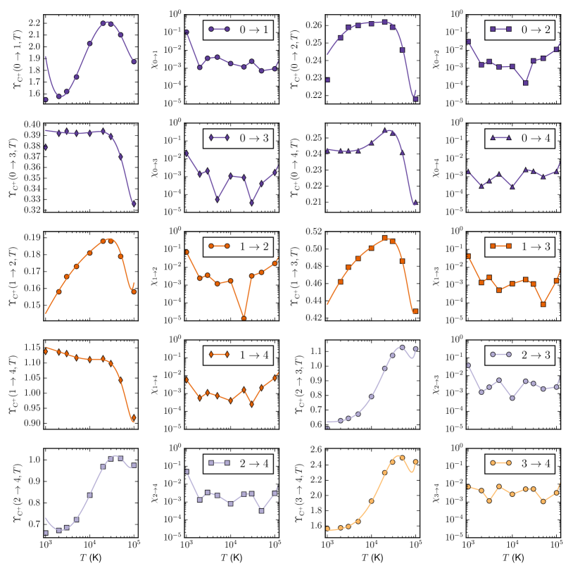
Figure 15: Fits for C⁺.

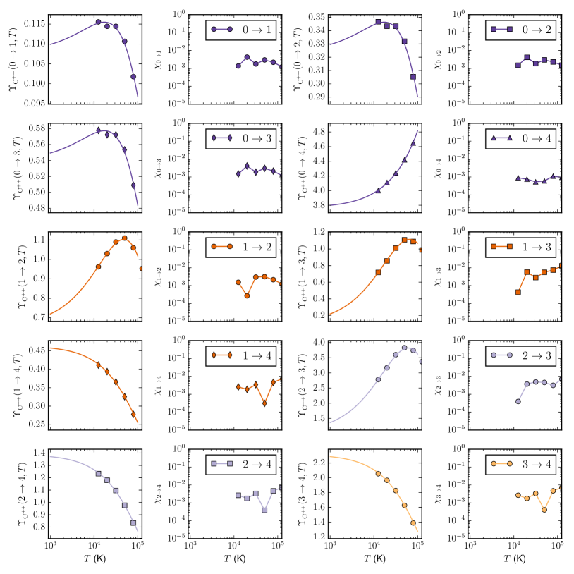
Figure 16: Fits for C⁺⁺.

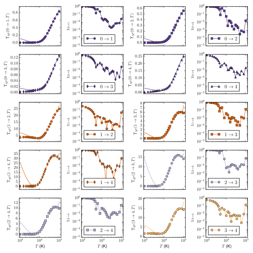
Figure 17: Fits for N⁰.

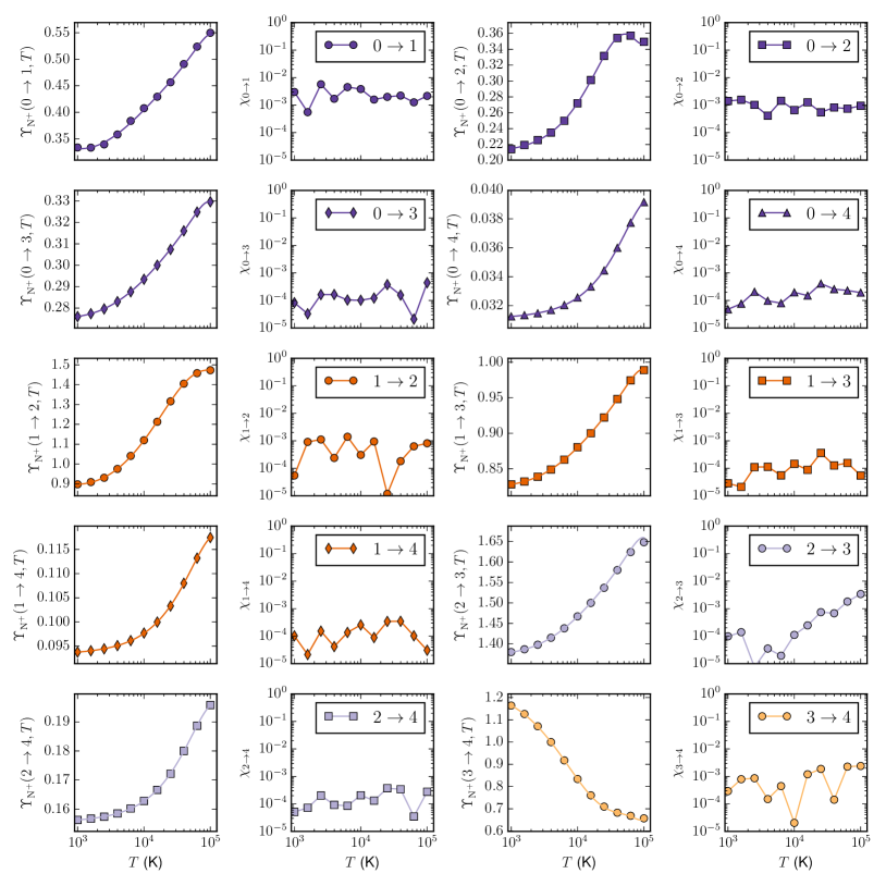
Figure 18: Fits for N⁺.

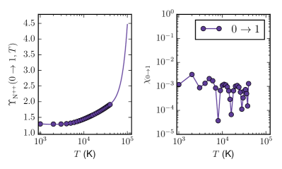
Figure 19: Fits for N⁺⁺.

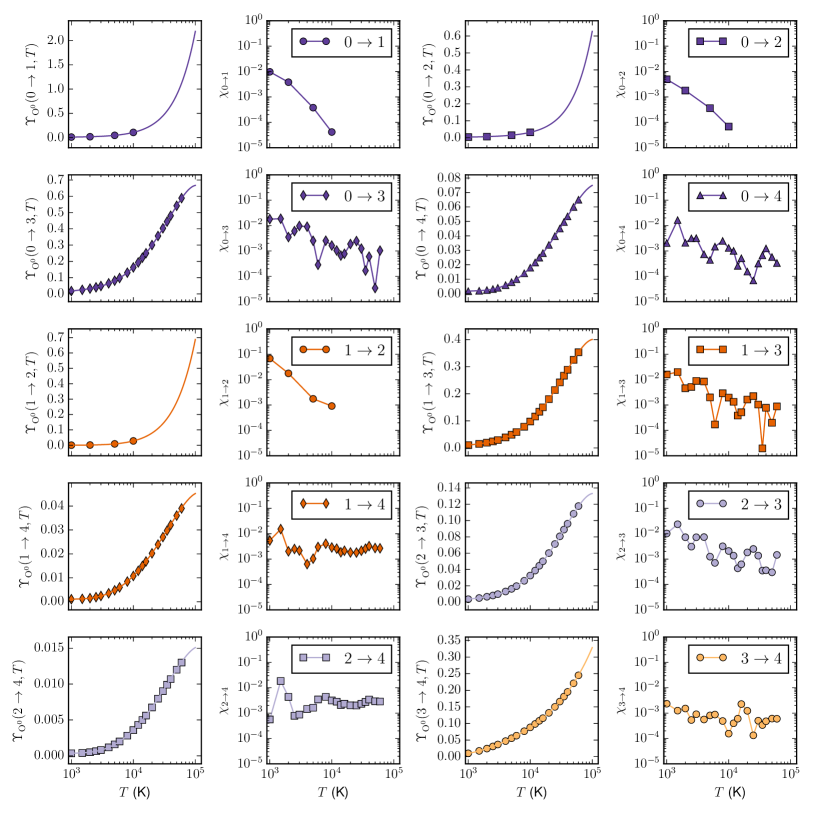
Figure 20: Fits for O⁰.

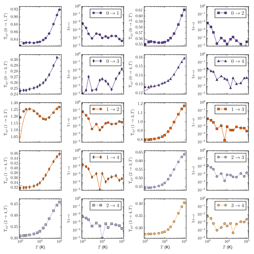
Figure 21: Fits for O⁺.

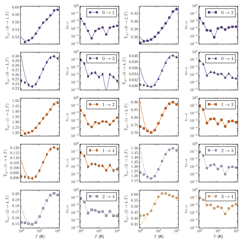
Figure 22: Fits for O⁺⁺.

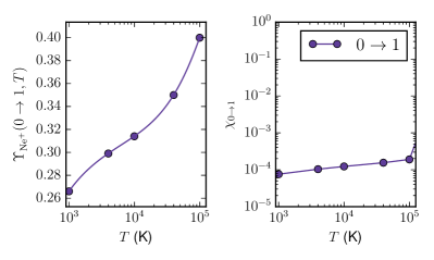
Figure 23: Fits for Ne⁺.

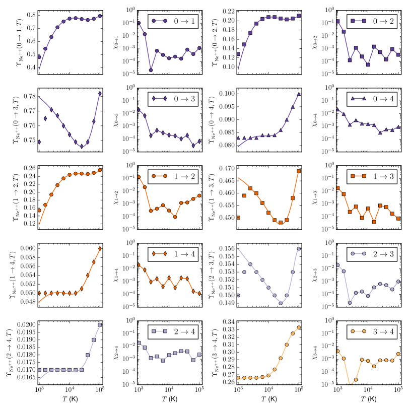
Figure 24: Fits for Ne⁺⁺.

The values of the fitting parameters are listed in Tables 9 - 13, the corresponding fits and relative differences between fit and data are shown in Figures 15 - 27.

2.4 Hydrodynamics

Hydrodynamical integration is performed using a finite volume method (Toro, 2009) on a generally unstructured, (co-)moving mesh (Springel, 2010). The Euler equations of hydrodynamics in conservative form

$$\frac{\partial{}U}{\partial{}t}+\vec{\nabla{}}.\vec{F}\left(U\right)=0,$$ (21)

with

$$U=\begin{pmatrix}\rho{}\\ \vec{v}\\ P\end{pmatrix},$$ (22)

$$\vec{F}(U)=\begin{pmatrix}\rho{}\vec{v}\\ \rho{}\vec{v}\vec{v}+P\vec{\vec{1}}\\ \rho{}\left(u+\frac{1}{2}\left|\vec{v}\right|^{2}\right)+P\vec{v}\end{pmatrix},$$ (23)

and an adiabatic equation of state $P=\left(\gamma{}-1\right)\rho{}u$, where $\rho{}$ is the mass density, $\vec{v}$ the flow velocity, $P$ the pressure, and $u$ the thermal energy per unit mass, are discretized on an unstructured Voronoi mesh. Integration of the primitive variables over the volume $V_{i}$ of each cell leads to a set of conserved variables (mass $m_{i}$, momentum $\vec{p}_{i}$, and total energy $E_{i}$) for each cell. Integrating the conservation law (21) over the volume of the cell allows us to reduce the time integration of these conserved quantities as a flux exchange between the cell and its neighbouring cells:

$$\frac{\text{d}Q_{i}}{\text{d}t}=-\sum_{j}\vec{F}_{ij}.\vec{A}_{ij},$$ (24)

where $\vec{A}_{ij}$ represents the oriented surface area of the geometrical face between cell $i$ and cell $j$, $\vec{F}_{ij}$ is an appropriate estimate of the fluxes (23) at a representative location on the face, and $Q_{i}$ is the vector of conserved variables for that cell.

To obtain appropriate fluxes, we use the values on both sides of the face as input for an exact Riemann solver, which gives the exact physical solution for the two state problem defined by the variables at both sides up to a desired precision. By sampling this analytic solution we obtain new values for the primitive variables that can be used to compute fluxes to be used in (24).

Note that our current implementation is only first order in space and time. It is however very straightforward to extend this to higher order by the introduction of appropriate spatial gradients, see e.g. Vandenbroucke and De Rijcke (2016); this will be implemented in future versions of the code. Our current implementation also does not yet include external forces or self-gravity.

2.4.1 Moving mesh scheme

For the specific case of an unstructured Voronoi grid, we can make the method Lagrangian by allowing the generators of the Voronoi grid to move in between time steps of the integration scheme. To account for this movement, we add correction terms to the flux expressions (23), as detailed in (Springel, 2010; Hopkins, 2015; Vandenbroucke and De Rijcke, 2016). Note that the hydrodynamical integration is completely independent of the movement of the generators. If the generators do not move, the method is Eulerian. If on the other hand the generator movement is set to the local fluid velocity in the corresponding cell, the method is fully Lagrangian. In the latter case, we can solve the Riemann problem across the cell faces in the rest frame of the faces, which leads to better accuracy in the presence of large bulk velocities, and allows us to use a larger integration time step than would be used in an equivalent Eulerian scheme, as the time step only depends on the relative velocity of the fluid w.r.t. the grid.

2.4.2 Radiation hydrodynamics

To couple the radiation to the hydrodynamics, an operator splitting method is used, whereby the photoionization heating term is added after each step of the hydrodynamics scheme, assuming photoionization equilibrium. The current values of the density in each cell are converted into number densities that are then used as input for the photoionization code. The photoionization code computes a self-consistent ionization structure for each cell, which is then used to decide what the temperature of the cell should be. The number of iterations and number of photon packets used in this step is a simulation parameter. The resulting temperature is compared with the actual hydrodynamical temperature of the cell, and the energy difference is added to the cell as an energy source term.

In our current implementation, we do not subtract energy for cells that were ionized and become neutral again, since this involves a careful treatment of the time step to prevent negative energies. We use an almost isothermal equation of state with an adiabatic index $\gamma{}=1.0001$, and assume a two-temperature medium, whereby the temperature in the neutral phase is assumed to be $T_{n}=100\leavevmode\nobreak\ {\rm{}K}$, while the temperature in the ionized medium is assumed to be $T_{i}=10,000\leavevmode\nobreak\ {\rm{}K}$. For a cell with hydrogen neutral fraction $x_{\rm{}H}$, the assumed average temperature is then

$$T=x_{\rm{}H}T_{n}+\left(1-x_{\rm{}H}\right)T_{i}.$$ (25)

This approach is sufficient to reproduce a basic benchmark expansion test (see 4.3). We could of course also get the photoionization heating directly from the photoionization step; this more general approach will be subject of future work.

Note that it is possible to couple CMacIonize as an external library to other hydrodynamics codes using a very similar approach, see 3.3.

3 Code

The most important difference between CMacIonize and the original photoionization code of Wood et al. (2004) is a complete redesign of the structure of the code (accompanied by a migration from Fortran to C++11), including a full in-line documentation of the code using Doxygen (the documentation for the latest stable version of the code can be found on a dedicated webpage). Below we outline the main design considerations and detail how they are implemented in the code.

3.1 Design considerations

3.1.1 User friendliness

The photoionization part of CMacIonize is primarily focused on post-processing output from other simulation codes as part of a simulation analysis work flow. This means that the code will be used by researchers that are not necessarily very familiar with the details of the code, but that still want to produce reproducible science products. To accommodate this, we aim to minimize the learning curve for using CMacIonize. In cases where writing additional code is inevitable (like for example when reading a new type of input file), we want to limit the effort necessary to accomplish this: the new code should be limited to a single function or C++ class, and the user should be able to write this code without worrying about the details of the photoionization algorithm.

3.1.2 Reproducibility

A properly designed computer algorithm should be deterministic, so that running the same simulation twice with the same input and the same version of a code should produce exactly the same result, independent of the hardware architecture. Parallelization and system specific optimizations might cause tiny changes in round off that could cause minuscule changes in result between different runs (especially in Monte Carlo algorithms), but even then a simulation code should be very close to a unique mapping from input data to an output solution. Reproducibility is hence an inherent feature of computer simulations.

However, keeping track of input parameters and code versions can be tedious, especially when simulations are combined with the design of improved algorithms and code changes are made. For this reason, we aim to provide a robust system to log parameters and code versions, so that all published CMacIonize results should be perfectly reproducible.

3.1.3 Modularity

Complex algorithms combine a large number of components that each have their specific complexities. However, most of these components are predominantly independent of each other, and only interact with the other components through narrowly defined interfaces. Isolating complex components into separate entities or modules increases the readability of a code, and makes the code more robust if combined with an appropriate unit testing strategy. We will therefore aim to produce a modular code, whereby separate components are identified and isolated into separate code entities.

3.1.4 Scalability

Modern computing architecture is highly parallel, with the computing power of a typical high performance computer spread out over a large number of separate computing units or nodes that are interconnected through a high speed network, and with each of these nodes in turn consisting of up to 128 separate CPU cores that share a single memory space. In order to efficiently use these machines, it is crucial that an algorithm is designed with a parallel mindset. We cannot think of the algorithm as a serial list of instructions that are executed one by one, but instead need to think of the tasks that need to be performed by the algorithm, the data that is needed to perform these tasks (and that might be shared with other tasks), and the dependencies that govern which tasks can be executed in parallel and which tasks are mutually exclusive due to conflicts.

In the current version of CMacIonize, we aim to provide a reasonable scaling by distributing computations across multiple cores on a single node, and across multiple nodes. Our current parallelization strategy does not address the need to distribute data across multiple nodes in order to efficiently use the available memory. This will be addressed in future versions of the code.

3.2 Design implementation

3.2.1 User interface

For standard users that do not plan to add additional code, the interaction with CMacIonize is limited to

• calling the command line program CMacIonize, and

• writing a parameter file that contains the parameters for the simulation.

The command line program has a very limited set of options that control the number of shared memory parallel threads used to run, and the mode in which to run (photoionization only or RHD). The only other parameter to the program is the name of the parameter file. An example command line call to CMacIonize could like this:

./CMacIonize --params parameterfile.param \
             --threads 8

This will run CMacIonize in the standard photoionization mode using 8 shared memory parallel threads, and using the parameters provided in the file parameterfile.param.

The parameter file contains all information needed to set up and run the simulation, and maps to the underlying modular structure of the code (all parameters are linked to a specific C++ class). It is a simple text file in YAML format, and a very basic example could look like this:

SimulationBox:
  anchor: [-5. pc, -5. pc, -5. pc]
  sides: [10. pc, 10. pc, 10. pc]
  periodicity: [false, false, false]

DensityGrid:
  type: Cartesian
  number of cells: [64, 64, 64]

DensityFunction:
  type: Homogeneous
  density: 100. cm^-3
  temperature: 8000. K

PhotonSourceDistribution:
  type: SingleStar
  position: [0. pc, 0. pc, 0. pc]
  luminosity: 4.26e49 s^-1

PhotonSourceSpectrum:
  type: Monochromatic
  frequency: 13.6 eV

IonizationSimulation:
  number of photons: 1e6
  number of iterations: 20

This parameter file sets up a Strömgren test in a box of $10\leavevmode\nobreak\ {\rm{}pc}\times{}10\leavevmode\nobreak\ {\rm{}pc}\times{}10\leavevmode\nobreak\ {\rm{}pc}$ containing gas with a density of $100\leavevmode\nobreak\ {\rm{}cm}^{-3}$ at a temperature of 8,000 K, with a star at the centre with a total luminosity of $4.26\times{}10^{49}\leavevmode\nobreak\ {\rm{}s}^{-1}$ and a monochromatic spectrum with a frequency equivalent to a photon of $13.6\leavevmode\nobreak\ {\rm{}eV}$. The simulation uses a Cartesian grid of $64\times{}64\times{}64$ cells, and uses 20 iterations with $10^{6}$ photon packets for each iteration (see 4.1 for details of this test).

The example above illustrates how easy it is to read and understand a parameter file. It also illustrates another key feature of the code: the use of units. Internally, we consistently use SI units throughout the code to avoid any confusion about units. However, we also require the user to specify units for all physical quantities that are used as an input, so that the user does not need to worry about unit conversions at all. We support a variety of different units, including complex unit conversions (e.g. photon energy in eV to photon frequency in Hz), and adding new units is very straightforward.

Apart from supporting units, the parameter file also supports various number formats and 3D vectors.

When the program is started, the parameter file is parsed and translated into a corresponding simulation structure. Before the actual simulation starts, the actually used parameters are written to a reference file. Most parameters have default values and need not be specified in the parameter file; when written to the reference file, the default values will be displayed, and the file will clearly state that the default value was used. If a parameter is not used, the reference file will mention this as well. For parameters that have units, the reference file will contain the value in SI units, as well as the original value.

If no parameter file is given, default values will be used for all parameters (that correspond to a low resolution version of the Strömgren benchmark test, see 4.1). In this case it is possible to use the reference file as a first guess for sensible parameter values, and iterate on it to construct an actual useful parameter file. All available parameters are also extensively documented in the Doxygen documentation of the corresponding classes.

3.2.2 Reproducibility

In order to guarantee reproducibility, we use a strategy that consists of three pillars:

1. version control as a way to uniquely identify a specific code version,

2. parameter logging in output files as a way to keep track of used parameters, and

3. unit testing to guarantee the same results across code versions.

Version control

The code is stored in a public online Git repository to make it easier to keep track of the code history, and to facilitate collaboration on the code. Git keeps track of the changes that are made to the code in between so called commits, i.e. logged checkpoints of the code status. Each commit has an associated key that uniquely identifies it, and it is always possible to return to a specific version of the code using the appropriate commit key.

Moreover, Git also provides a command line tool called git describe that can be used to check the current version of the local copy of the repository that a user is using, and that checks if the repository is dirty, i.e. contains uncommitted code changes.

We have incorporated git describe into our code configuration chain, so that the compiled code knows (a) what the unique commit key of the current version is, and (b) if the current code version is exactly equal to that code version, or contains uncommitted changes. If the code contains uncommitted changes, it will refuse to run any simulation, so that the user is forced to commit changes and make sure the code is identifiable before running scientific simulations.

Logging

The output of any simulation consists of snapshots, i.e. dumps of specific quantities at some time during the simulation. CMacIonize supports various types of snapshot files, the default being the same HDF5 format that is also used by Gadget2 ascl:0003.001, SWIFT, and Shadowfax.

In order to exactly reproduce a snapshot file, we need to know

• what version of the code was used to generate it, and

• which parameters were used to run the code.

The former can be easily realised by storing the unique commit key for the current code version in the snapshot files. To guarantee the latter, we also store all parameters in the snapshot files, as they were used. This corresponds to the values that are part of the reference parameter file (see 3.2.1). By also storing the parameters for which default values were used, we guarantee reproducibility across different code versions, if at some point the default value for a parameter were to change. The public version of the code contains a Python script that can extract the parameter file that was used from a snapshot file in the default HDF5 format.

For simulations that use input from external files, as e.g. simulations that post-process the density field from another simulation, we also need these external files in order to reproduce the results. Since these files can be quite large, storing them as part of the snapshot files is not an option. In this case, we rely on the user using a convenient method of keeping track of those files to guarantee reproducibility.

Apart from the code version and the parameter values we also log configuration flags and system specific information. This is not strictly necessary in order to reproduce simulation results, but might nonetheless be helpful e.g. during debugging.

Unit testing

One of the key issues when developing a simulation code is making sure that the results are scientifically accurate, and that they stay accurate throughout the further development of the code. Unit testing is a very powerful tool to achieve this, especially when combined with a good modular design (see 3.2.3).

A unit test is a small independent program that calls a small part of the code with known input values and checks its output against a known solution. If the output matches the expected result, the test passes and we know that part of the code behaves as expected.

When properly designed, a unit test covers all possible paths through the code that is being tested, e.g. if the code contains conditions that check for strange input values, the test will call the code with strange input values and check that these are handled correctly.

Unit tests were an integral part of the early development process of CMacIonize, as all new code was tested against reference values of the old code of Wood et al. (2004). During the addition of new features that were not part of the old code, we still tried to start from the unit test as much as possible, which meant first thinking about what the expected behaviour of a code component (function or class) should be, before actually implementing it. The overhead this implies is quickly recovered by the ease with which we can locate bugs in new code.

The current version of the code contains almost 70 separate unit tests, which are managed as part of our code configuration and run using CTest, the CMake unit testing framework. Depending on the hardware and system configuration, the tests take less than a minute to a few minutes to complete, and can be run as part of the standard compilation process.

When new code is added to the stable version on the Git repository, the new code is automatically compiled with a number of different compilers on different systems using the continuous integration environment Travis CI, and the unit tests are run. Code is only allowed to be merged into the stable repository if it passes all the tests. This way we ensure that new code never breaks or alters old functionality, unless this is done on purpose (in which case the corresponding unit test needs to be modified).

3.2.3 Object oriented design

To implement modularity in our code design, we use C++ objects as the building blocks of the code. An object has a limited number of responsibilities, and is as unaware as possible of the rest of the code (unless the interaction of various objects is the responsibility of the class). Most objects are covered by a corresponding unit test (see 3.2.2), although the unit tests for some classes are grouped together if this makes more sense.

We use a number of different design patterns (Gamma et al., 1995). Basic simulation components like the density grid and the source distribution use inheritance combined with a factory class to provide different interchangeable implementations (e.g. the density grid can be a regular Cartesian grid, an AMR mesh, or an unstructured Voronoi grid). The density grid itself makes extensive use of iterators to provide grid type unaware access to cells, while most grid computations are performed using visitors that perform a single task for each cell of the grid.

The object oriented design is tightly interwoven with the parameter file used as the user interface (see 3.2.1), with objects mapping to specific blocks in the parameter file (and the type keyword always referring to a factory class that provides multiple implementations of a general interface). Most objects have a so-called parameter file constructor, which can create an object instance based on the parameter values given in the parameter file, with parameters mapping directly to object properties.

3.2.4 Task based design

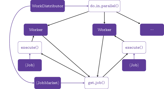
Figure 1: Schematic representation of a typical shared memory parallel run. A WorkDistributor spawns a number of parallel Worker objects that get tasks from a template JobMarket object that acts as a taskpool. The different threads keep drawing tasks from the pool until all tasks have been executed.

To provide inherent parallelism in our code, we think of the actions that need to be performed by the algorithm in terms of small tasks, that perform a limited set of actions on a small part of the computational domain. By limiting the amount of work done by a single task, we can improve the load balancing between different parallel threads significantly, while limiting the fraction of the computational domain that is affected minimizes conflicts.

The photon traversal algorithm e.g. can be done independently for small batches of photons. Each part of the path of a photon is only a single cell, so that we only need to worry about two threads accessing the same cell at the same time to prevent conflicts. Similarly, the ionization balance computation for different cells can be done completely independently, and so can the temperature balance computation or even the cell initialization.

In practice, our task based design is implemented using a number of interacting classes called Worker, Job, and JobMarket. Job and JobMarket make use of compile time polymorphism and are template interfaces, meaning that these classes do not actually exist, but are abstract interfaces that define common functionality for classes that can be used as C++ template arguments for other classes. This offers the same flexibility as run time polymorphism, but without the computational overhead. A Worker is our abstract representation of a thread, while a Job is the abstract representation of a task that needs to be performed. The JobMarket is responsible for spawning Job instances. The Worker instances in turn are spawned by a WorkDistributor, which is the only class that needs to know about the underlying parallel environment that is used. Our current implementation only supports OpenMP, but it would be straightforward to replace this by e.g. a POSIX threads or Intel Threading Building Blocks implementation.

The general workflow for a shared memory parallel run is illustrated in Figure 1. When a parallel part of the execution is started, a corresponding JobMarket implementation is created and passed on as a template argument to the WorkDistributor. The WorkDistributor then generates a number of Worker instances that are run in parallel, and that call the get_job() function of the JobMarket instance to get actual Job instances that need to be executed. The worker then calls the execute() method of the Job instance to perform the task at hand. When the task is finished, the Worker goes back to the JobMarket to get the next Job, until no more tasks are available.

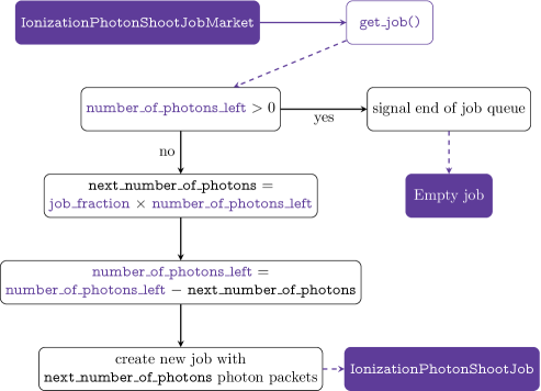
Figure 2: JobMarket implementation that controls the load balancing of a parallel photoionization run. We create a new Job instance that will propagate a fraction of the total number of photons left to propagate. This ensures that tasks gradually get smaller, which in turn guarantees a minimal load imbalance, as the maximal load imbalance is the time it takes to execute a single task. Note that this function is not thread safe and hence requires a locking mechanism to ensure safe access.

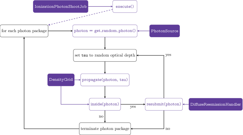
Figure 3: Job implementation that propagates a number of photons through the grid. Note that the call to DensityGrid::propagate requires a locking mechanism for thread safe cell access (the rest of the function is thread safe).

This paradigm nicely divides the responsibilities of the parallelization process: the Job provides the actual task at hand, the JobMarket regulates how tasks are divided and hence controls the load balancing, while the WorkDistributor is responsible for handling the underlying parallel environment. Figure 2 and Figure 3 show how this works for a photoionization simulation.

We need a locking mechanism to protect common variables in the shared memory domain, like e.g. cells in the photon traversal algorithm or counter values within the JobMarket. To this end, we provide our own Lock class that is unaware of the underlying parallel environment. We also experimented with using atomic data operations, but found this to be slower than a locking mechanism in most cases, predominantly because of the lack of hardware support for floating point atomic operations, and because the large number of variables updated per cell access in the photon traversal algorithm reduces the impact of using an expensive locking mechanism.

3.3 Library exposure

To improve the usability of CMacIonize, we also provide a library interface to the code, which can be used in both C, C++ and Fortran2003. This library interface is in all ways equivalent to the standard CMacIonize program (the same IonizationSimulation class is used to run an actual photoionization simulation), but uses special input and output classes to directly obtain the density field from another code and return the resulting ionization structure to that code without the need to output anything to disk.

Our current library implementation has already successfully been used to couple the code to the SPH code PHANTOM ascl:1709.002.

The library needs to be initialized using a parameter file that is identical to the one used for the actual CMacIonize program, and provides a single function that takes an array of positions, smoothing lengths and masses as an input, and outputs an array of neutral hydrogen fractions. Under the hood, it converts the positions, smoothing lengths and masses into a density field that is mapped onto a density grid, and then uses sources from the parameter file to illuminate this density field and compute self-consistent neutral fractions. These neutral fractions are then mapped back to the original SPH positions using the provided smoothing lengths.

It should be fairly straightforward to use the same approach to couple the code to other types of hydrodynamical codes, like AMR codes.

Some parts of the code are also wrapped into a Python library. This library is not meant to run full photoionization simulations like the C/C++/Fortran counterpart, but instead can be used to facilitate the analysis of simulation snapshots, by e.g. providing access to the line cooling data used by the code.

3.4 Unstructured grid generation

An important feature of CMacIonize is the option to use an unstructured Voronoi grid as the main grid structure for both the radiation transfer and the hydrodynamics. Due to the poor scaling properties of the incremental construction algorithm used in Vandenbroucke and De Rijcke (2016), we decided to implement two new algorithms. The first algorithm (which for historical reasons is called the “old” Voronoi algorithm) is our own rewritten version of the no longer actively supported voro++ library. This algorithm works in most cases. However, we found that in some very specific degenerate cases, the voro++ algorithm can produce the wrong Voronoi grid without crashing (as can be confirmed graphically, or by computing the total volume of all cells). This is due to the way the algorithm handles degeneracies.

Since these degenerate cases do in fact happen when starting a moving-mesh hydrodynamical simulation from a regular initial grid, we also implemented a new, more scalable version of the incremental construction algorithm used in Shadowfax (called the “new” algorithm). The current version of this grid construction algorithm is about a factor 3 slower than the voro++ algorithm, but is completely robust to any degeneracies due to the usage of arbitrary precision arithmetics. We plan to release this algorithm as a standalone library that can be used as a replacement for voro++ (Vandenbroucke et al., in prep.).

In this work, we will use the old Voronoi algorithm whenever an unstructured grid is used. This does not affect the results we show in any way, as the Voronoi grid for a set of points is a unique geometrical structure, and is independent of the way it is computed.

4 Benchmarks

In order to verify that our code produces physically accurate results in an efficient way, we run a number of benchmark tests. Tests are grouped together into four categories:

1. tests that verify the ionization algorithm,

2. tests that verify the combined ionization and temperature computation algorithm,

3. tests that verify the radiation hydrodynamics algorithms, and

4. tests that check the parallel efficiency of the code.

For the fourth category, we just reuse tests from the three other categories. The initial conditions and analysis scripts for all benchmark tests are part of the public version of the code.

4.1 Strömgren sphere

To test the ionization algorithm, we run a simple test, inspired by the work of Strömgren (1939), in which a single ionizing source is at the centre of a box containing a homogeneous density field consisting of only hydrogen. If we assume that the source completely ionizes all hydrogen within a radius $R_{s}$ (the Strömgren radius), while the hydrogen outside this region stays neutral, then the ionization balance equation for the ionized region is (Osterbrock and Ferland, 2006):

$$Q=\frac{4\pi{}}{3}R_{s}^{3}n_{\text{H}}^{2}\alpha{}_{\text{H}^{+}\rightarrow{}\text{H}^{0}}(T),$$ (26)

where we made the assumption that $n_{\text{H}}=n_{\text{H}^{+}}$ within the ionized region. If we also assume a fixed temperature $T_{0}$, then we get an analytic expression for the constant Strömgren radius:

$$R_{s}=\left(\frac{3Q}{4\pi{}n_{\text{H}}^{2}\alpha{}_{\text{H}^{+}\rightarrow{}\text{H}^{0}}(T_{0})}\right)^{\frac{1}{3}}.$$ (27)

If the ionized region itself emits ionizing radiation (through the diffuse field), the ionization balance equation changes to

$$Q\left(1+P_{r,\text{H}}(T)+P_{r,\text{H}}(T)^{2}+...\right)\\ =\frac{4\pi{}}{3}R_{s}^{3}n_{\text{H}}^{2}\alpha{}_{\text{H}^{+}\rightarrow{}\text{H}^{0}}(T),$$ (28)

where $P_{r,\text{H}}(T)$ is the reemission probability for ionizing radiation.

Using $1+x+x^{2}+...=\frac{1}{1-x}$, (27) now becomes:

$$R_{s}^{\prime}=\left(\left(\frac{Q}{1-P_{r,\text{H}}(T_{0})}\right)\frac{3}{4\pi{}n_{\text{H}}^{2}\alpha{}_{\text{H}^{+}\rightarrow{}\text{H}^{0}}(T_{0})}\right)^{\frac{1}{3}}.$$ (29)

We will hence run two different versions of the test, that test different parts of the algorithm:

1. a version that does not include the diffuse reemission field and should reproduce (27), and

2. a version that includes diffuse radiation and should produce a larger ionization region, as given by (29).

For both tests, we will use a cubic box of $10\times{}10\times{}10$ pc containing gas with a hydrogen number density of $n_{\text{H}}=100\leavevmode\nobreak\ \text{cm}^{-3}$. At the centre of the box, we put a single source with a luminosity of $Q=4.26\times{}10^{49}\leavevmode\nobreak\ \text{s}^{-1}$ with a monochromatic spectrum that emits photons at the ionization threshold energy for hydrogen, $\nu{}=13.6\leavevmode\nobreak\ \text{eV}$. We assume a constant photoionization cross section for neutral hydrogen of $\sigma{}_{\text{H}^{0}\rightarrow{}\text{H}^{+}}=6.3\times{}10^{-18}\leavevmode\nobreak\ \text{cm}^{-2}$, and a constant radiative recombination rate $\alpha{}_{\text{H}^{+}\rightarrow{}\text{H}^{0}}(T_{0})=4\times{}10^{-13}\leavevmode\nobreak\ \text{cm}^{3}\leavevmode\nobreak\ \text{s}^{-1}$. The abundances, photoionization cross sections and recombination rates for all other elements and ions are set to zero.

We use a Cartesian density grid of $64\times{}64\times{}64$ cells, and use $10^{6}$ photon packets for 20 iterations to get a converged result.

4.1.1 No diffuse field

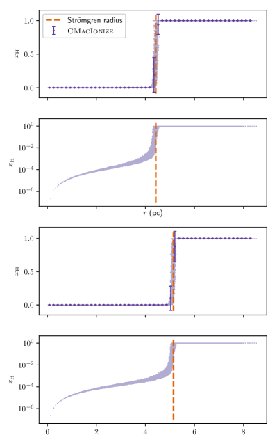
Figure 4: Hydrogen neutral fraction as a function of radius for the two versions of the Strömgren benchmark test. Top panels: version without diffuse radiation, bottom panels: version with diffuse radiation. The light purple dots show the simulation results for the individual cells; the dark purple error bars show the same results in 50 radial bins, with the size of the error bars showing the scatter within the bin. The orange dashed line is the corresponding analytic Strömgren radius. For clarity, the results are shown on both a linear and a logarithmic scale.

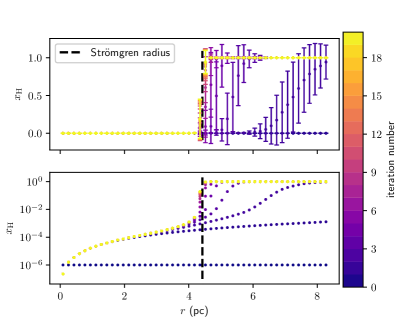
Figure 5: Hydrogen neutral fraction as a function of radius for the benchmark test without diffuse field, for different iteration numbers. For clarity, we only show the binned results, with the size of the error bar representing the scatter within the bin. The black dashed line is the analytic Strömgren radius. On the bottom panel we show the same results on a logarithmic scale without the error bars.

This test corresponds to the benchmark test stromgren, and the setup is as described above. The resulting hydrogen neutral fraction as a function of radius is shown in the top panel of Figure 4. The code accurately reproduces the expected Strömgren radius given by (27).

Figure 5 shows the evolution of the hydrogen neutral fraction profile with the number of iterations used. Initially, the neutral fraction is set to a very low value everywhere in the box, so that the ionizing radiation can illuminate a large region efficiently. After the first iterations of the ionization state computation, the neutral fraction in the outer regions quickly goes up until a converged result is reached. The result is already well converged after 6 iterations.

4.1.2 Diffuse field

This test corresponds to the benchmark test stromgren_diffuse, and includes diffuse reemission with a reemission probability $P_{r,\text{H}}(T_{0})=0.364$ (corresponding to $T_{0}=8000\leavevmode\nobreak\ \text{K}$). The resulting hydrogen neutral fraction profile is shown in the bottom panel of Figure 4. As expected, the ionized region is larger in this case. Our code still accurately reproduces the expected Strömgren radius given by (29).

4.2 Lexington benchmarks

To test the combined temperature and ionization calculation for the full system including metals, we run two of the benchmark tests that were the result of a 1995 workshop in Lexington and that are known as the Lexington benchmarks (Ferland, 1995). The initial conditions for these tests can be found in Péquignot et al. (2001), and correspond to the HII40 and HII20 model in that work.

The tests consist of a uniform density box with a hydrogen number density $n_{\text{H}}=100\leavevmode\nobreak\ \text{cm}^{-3}$, in which a central spherical region with radius $R_{\text{in}}=3\times{}10^{16}\leavevmode\nobreak\ \text{m}$ is evacuated. In the centre of the evacuated region we place a single stellar source with a luminosity $Q=10^{49}\leavevmode\nobreak\ \text{s}^{-1}$ for the low temperature benchmark, and $Q=4.26\times{}10^{49}\leavevmode\nobreak\ \text{s}^{-1}$ for the high temperature benchmark, with a black body spectrum. The temperature $T_{\text{BB}}$ of the black body spectrum is also different for the two tests, with $T_{\text{BB}}=20,000\leavevmode\nobreak\ \text{K}$ for the low temperature benchmark, and $T_{\text{BB}}=40,000\leavevmode\nobreak\ \text{K}$ for the high temperature version. The abundances (relative to hydrogen) of helium and the various coolants are set to the values listed in Table 2.

Table 2: Abundances for helium and the different coolants in the Lexington benchmark tests.

element	abundance
He/H	$0.1$
C/H	$2.2\times{}10^{-4}$
N/H	$4\times{}10^{-5}$
O/H	$3.3\times{}10^{-4}$
Ne/H	$5\times{}10^{-5}$
S/H	$9\times{}10^{-6}$

To compare the test results, a number of quantities are computed:

• The total H$\beta{}$ luminosity, which is computed from a power law fit to the data of Storey and Hummer (1995), using the electron density and temperature derived from the photoionization simulation.

• The height of the Balmer Jump $\Delta{}(BC\leavevmode\nobreak\ 3645)$, defined as the jump in the Balmer continuum flux in a synthetic spectrum between the flux at $3643\leavevmode\nobreak\ \text{\AA}$ and $3681\leavevmode\nobreak\ \text{\AA}$. To obtain synthetic spectra, we use the continuum emission coefficients for hydrogen and helium from Brown and Mathews (1970). Note that Péquignot et al. (2001) and other authors wrongly quote this value in units of Å, while the actual value is in $\text{\AA}^{-1}$.

• The inner temperature $T_{\text{inner}}$ at the boundary of the evacuated region.

• The average density weighted temperature (Ferland, 1995)

  $$\langle{}T[n_{e}n_{\text{H}^{+}}]\rangle{}=\frac{\int n_{e}n_{\text{H}^{+}}T\text{d}V}{\int n_{e}n_{\text{H}^{+}}\text{d}V}.$$ (30)

• The outer radius of the ionization region, defined as the average radius of cells with hydrogen neutral fractions in the range $f_{\text{H}^{0}}\in{}[0.1,0.2]$.

• The ratio of the density weighted ionized fractions of hydrogen and helium, defined as

  $$\frac{\langle{}f_{\text{He}^{+}}\rangle{}}{\langle{}f_{\text{H}^{+}}\rangle{}}=\frac{\int n_{e}f_{\text{He}^{+}}\text{d}V}{\int n_{e}n_{\text{H}^{+}}\text{d}V}.$$ (31)

Apart from those, we also compute the line strengths of a number of emission lines, relative to the total H$\beta{}$ luminosity. These lines are a subset of the emission lines that are used for the metal line cooling (see 2.3), and their strength is computed in the same way (summed over all cells).

For both tests, we set up a box of size $6\times{}6\times{}6\leavevmode\nobreak\ \text{pc}$, using a Cartesian density grid of $64\times{}64\times{}64$ cells. We use $10^{8}$ photons and 20 iterations to get a converged result for all coolants.

To set up the initial condition with a vacuum region in the centre, we use a special implementation of the DensityFunction used to set up the density field, called BlockSyntaxDensityFunction. This implementation uses a very simple geometrical block description of the initial condition, which is the same as used by the initial condition generator of Shadowfax (Vandenbroucke and De Rijcke, 2016).

4.2.1 Low temperature benchmark

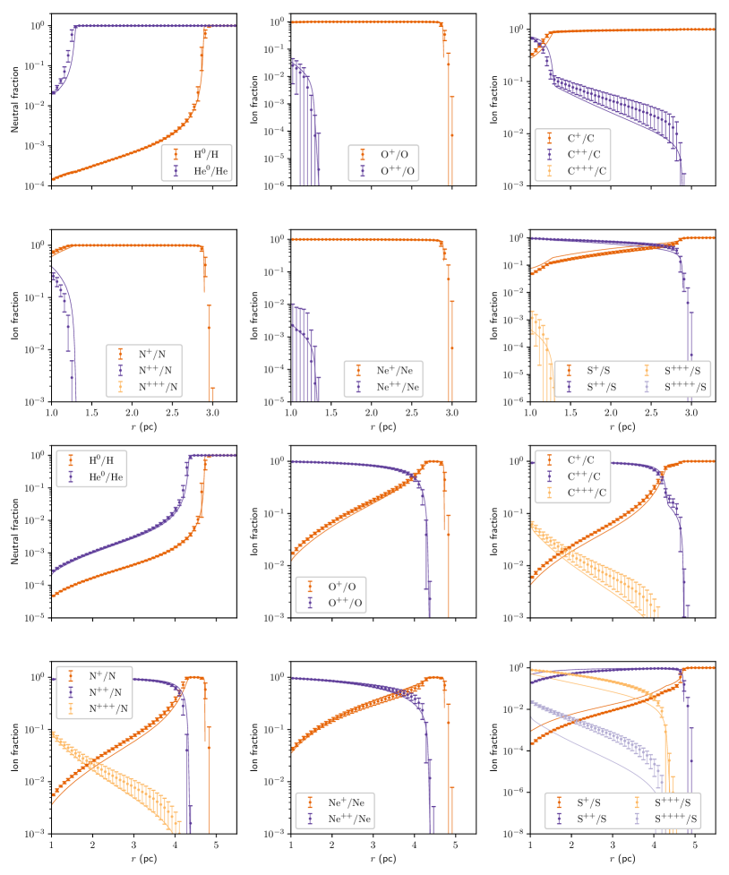
Figure 6: Ionic fraction of hydrogen, helium, and various coolants as a function of radius, as indicated on the figures. Top rows: low temperature benchmark, bottom rows: high temperature benchmark. The error bars show the simulation results, while the full lines are the equivalent Cloudy results.

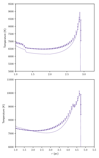
Figure 7: Temperature as a function of radius for the Lexington benchmarks. Top rows: low temperature benchmark, bottom rows: high temperature benchmark. The error bars show the simulation results, while the full line represents the equivalent Cloudy result.

This corresponds to the lexingtonHII20 benchmark test, and uses a black body spectrum with $T_{\text{BB}}=20,000\leavevmode\nobreak\ \text{K}$. The resulting ionic fraction profiles for hydrogen, helium and several coolants are shown in the top panel of Figure 6, together with reference values from the 1D code Cloudy. They follow the same trends as observed in e.g. Wood et al. (2004), and overall agreement is pretty good. The resulting temperature profile is shown in the top panel of Figure 7. Our result follows the same overall trend as the reference curve, but we systematically overestimate the temperature in the ionized region. We do reproduce the correct peak temperature at the ionization radius. This difference can be attributed to the different cooling rates we use compared to Cloudy.

Table 3 lists the line strengths and comparison quantities used by Péquignot et al. (2001), and compares them with the median values given in that paper. All values have the expected order of magnitude, although some values deviate significantly. This can be attributed to a combination of our overall higher temperature, and different line emission rates.

Table 3: Line strengths and comparison quantities for the low temperature Lexington benchmark test. P2001 denotes the median value as given in Péquignot et al. (2001).

Quantity	CMacIonize value	P2001 value
H$\beta{}$ luminosity	$4.81\times{}10^{36}\leavevmode\nobreak\ \text{erg}\leavevmode\nobreak\ \text{s}^{-1}$	$4.89\times{}10^{36}\leavevmode\nobreak\ \text{erg}\leavevmode\nobreak\ \text{s}^{-1}$
$\Delta{}(\text{BC}\leavevmode\nobreak\ 3645)$	$5.44\times{}10^{-3}\leavevmode\nobreak\ \text{\AA}^{-1}$	$5.56\times{}10^{-3}\leavevmode\nobreak\ \text{\AA}^{-1}$
$T_{\text{inner}}$	$7052\leavevmode\nobreak\ \text{K}$	$6789\leavevmode\nobreak\ \text{K}$
$\langle{}T[n_{e}n_{\text{H}^{+}}]\rangle{}$	$6843\leavevmode\nobreak\ \text{K}$	$6663\leavevmode\nobreak\ \text{K}$
$R_{\text{out}}$	$8.83\times{}10^{16}\leavevmode\nobreak\ \text{m}$	$8.89\times{}10^{16}\leavevmode\nobreak\ \text{m}$
$\langle{}f_{\text{He}^{+}}\rangle{}/\langle{}f_{\text{H}^{+}}\rangle{}$	0.047	0.049
Line	CMacIonize line strength	P2001 line strength
$[\text{C\leavevmode\nobreak\ II}]$ $2325\leavevmode\nobreak\ \text{\AA}$ multiplet	0.066	0.047
$[\text{N\leavevmode\nobreak\ II}]$ $122\leavevmode\nobreak\ \mu{}\text{m}$	0.068	0.071
$[\text{N\leavevmode\nobreak\ II}]$ $6584\leavevmode\nobreak\ \text{\AA}$ and $6548\leavevmode\nobreak\ \text{\AA}$	0.845	0.803
$[\text{N\leavevmode\nobreak\ II}]$ $5755\leavevmode\nobreak\ \text{\AA}$	0.0029	0.0029
$[\text{N\leavevmode\nobreak\ III}]$ $57.3\leavevmode\nobreak\ \mu{}\text{m}$	0.0030	0.0031
$[\text{O\leavevmode\nobreak\ I}]$ $6300\leavevmode\nobreak\ \text{\AA}$ and $6363\leavevmode\nobreak\ \text{\AA}$	0.0052	0.0060
$[\text{O\leavevmode\nobreak\ II}]$ $7320\leavevmode\nobreak\ \text{\AA}$ and $7330\leavevmode\nobreak\ \text{\AA}$	0.0103	0.0087
$[\text{O\leavevmode\nobreak\ II}]$ $3726\leavevmode\nobreak\ \text{\AA}$ and $3729\leavevmode\nobreak\ \text{\AA}$	1.33	1.10
$[\text{O\leavevmode\nobreak\ III}]$ $51.8\leavevmode\nobreak\ \mu{}\text{m}$	0.0013	0.0012
$[\text{O\leavevmode\nobreak\ III}]$ $88.3\leavevmode\nobreak\ \mu{}\text{m}$	0.0016	0.0014
$[\text{O\leavevmode\nobreak\ III}]$ $5007\leavevmode\nobreak\ \text{\AA}$ and $4959\leavevmode\nobreak\ \text{\AA}$	0.0018	0.0015
$[\text{Ne\leavevmode\nobreak\ II}]$ $12.8\leavevmode\nobreak\ \mu{}\text{m}$	0.297	0.271
$[\text{S\leavevmode\nobreak\ II}]$ $6716\leavevmode\nobreak\ \text{\AA}$ and $6731\leavevmode\nobreak\ \text{\AA}$	0.459	0.492
$[\text{S\leavevmode\nobreak\ II}]$ $4068\leavevmode\nobreak\ \text{\AA}$ and $4076\leavevmode\nobreak\ \text{\AA}$	0.014	0.017
$[\text{S\leavevmode\nobreak\ III}]$ $18.7\leavevmode\nobreak\ \mu{}\text{m}$	0.333	0.420
$[\text{S\leavevmode\nobreak\ III}]$ $33.6\leavevmode\nobreak\ \mu{}\text{m}$	0.558	0.750
$[\text{S\leavevmode\nobreak\ III}]$ $9532\leavevmode\nobreak\ \text{\AA}$ and $9069\leavevmode\nobreak\ \text{\AA}$	0.479	0.525

4.2.2 High temperature benchmark

This corresponds to the lexingtonHII40 benchmark test, and uses a black body spectrum with $T_{\text{BB}}=40,000\leavevmode\nobreak\ \text{K}$. The resulting ionic fraction profiles for hydrogen, helium and several coolants are shown in the bottom panel of Figure 6, and they again follow the same trends as observed in Wood et al. (2004). The resulting temperature profile is shown in the bottom panel of Figure 7. We again notice an overall higher temperature in most of the ionized region (although we actually underestimate the central temperature), which again is due to the different data values used by our code.

Table 4 lists the line strengths and comparison quantities. Note that we cannot compute the $[\text{C\leavevmode\nobreak\ II}]$ $1335\leavevmode\nobreak\ \text{\AA}$ line strength given in Péquignot et al. (2001), as this corresponds to a transition outside the five lowest lying levels of C⁺. Neither can we compute the $[\text{O\leavevmode\nobreak\ IV}]$ $25.9\leavevmode\nobreak\ \mu{}\text{m}$ line strength, since O⁺⁺ has an ionization potential that is (just) higher than the $54.4\leavevmode\nobreak\ \text{eV}$ upper limit of our energy interval, and we hence cannot track O⁺⁺⁺. The values generally agree with the Péquignot et al. (2001) values, although there are again significant differences, especially for the sulphur lines.

Table 4: Line strengths and comparison quantities for the high temperature Lexington benchmark test. P2001 denotes the median value as given in Péquignot et al. (2001).

Quantity	CMacIonize value	P2001 value
H$\beta{}$ luminosity	$2.01\times{}10^{37}\leavevmode\nobreak\ \text{erg}\leavevmode\nobreak\ \text{s}^{-1}$	$2.05\times{}10^{37}\leavevmode\nobreak\ \text{erg}\leavevmode\nobreak\ \text{s}^{-1}$
$\Delta{}(\text{BC}\leavevmode\nobreak\ 3645)$	$4.99\times{}10^{-3}\leavevmode\nobreak\ \text{\AA}^{-1}$	$4.97\times{}10^{-3}\leavevmode\nobreak\ \text{\AA}^{-1}$
$T_{\text{inner}}$	$7410\leavevmode\nobreak\ \text{K}$	$7663\leavevmode\nobreak\ \text{K}$
$\langle{}T[n_{e}n_{\text{H}^{+}}]\rangle{}$	$8127\leavevmode\nobreak\ \text{K}$	$8030\leavevmode\nobreak\ \text{K}$
$R_{\text{out}}$	$1.44\times{}10^{17}\leavevmode\nobreak\ \text{m}$	$1.46\times{}10^{17}\leavevmode\nobreak\ \text{m}$
$\langle{}f_{\text{He}^{+}}\rangle{}/\langle{}f_{\text{H}^{+}}\rangle{}$	0.784	0.770
Line	CMacIonize line strength	P2001 line strength
$[\text{He\leavevmode\nobreak\ I}]$ $5876\leavevmode\nobreak\ \text{\AA}$	0.116	0.116
$[\text{C\leavevmode\nobreak\ II}]$ $2325\leavevmode\nobreak\ \text{\AA}$ multiplet	0.184	0.140
$[\text{C\leavevmode\nobreak\ III}]$ $1907\leavevmode\nobreak\ \text{\AA}$ and $1909\leavevmode\nobreak\ \text{\AA}$	0.073	0.071
$[\text{N\leavevmode\nobreak\ II}]$ $122\leavevmode\nobreak\ \mu{}\text{m}$	0.029	0.033
$[\text{N\leavevmode\nobreak\ II}]$ $6584\leavevmode\nobreak\ \text{\AA}$ and $6548\leavevmode\nobreak\ \text{\AA}$	0.712	0.725
$[\text{N\leavevmode\nobreak\ II}]$ $5755\leavevmode\nobreak\ \text{\AA}$	0.0056	0.0052
$[\text{N\leavevmode\nobreak\ III}]$ $57.3\leavevmode\nobreak\ \mu{}\text{m}$	0.304	0.297
$[\text{O\leavevmode\nobreak\ I}]$ $6300\leavevmode\nobreak\ \text{\AA}$ and $6363\leavevmode\nobreak\ \text{\AA}$	0.0091	0.0087
$[\text{O\leavevmode\nobreak\ II}]$ $7320\leavevmode\nobreak\ \text{\AA}$ and $7330\leavevmode\nobreak\ \text{\AA}$	0.031	0.030
$[\text{O\leavevmode\nobreak\ II}]$ $3726\leavevmode\nobreak\ \text{\AA}$ and $3729\leavevmode\nobreak\ \text{\AA}$	2.19	2.12
$[\text{O\leavevmode\nobreak\ III}]$ $51.8\leavevmode\nobreak\ \mu{}\text{m}$	1.21	1.06
$[\text{O\leavevmode\nobreak\ III}]$ $88.3\leavevmode\nobreak\ \mu{}\text{m}$	1.43	1.23
$[\text{O\leavevmode\nobreak\ III}]$ $5007\leavevmode\nobreak\ \text{\AA}$ and $4959\leavevmode\nobreak\ \text{\AA}$	2.46	2.20
$[\text{O\leavevmode\nobreak\ III}]$ $4363\leavevmode\nobreak\ \text{\AA}$	0.0043	0.0040
$[\text{Ne\leavevmode\nobreak\ II}]$ $12.8\leavevmode\nobreak\ \mu{}\text{m}$	0.180	0.194
$[\text{Ne\leavevmode\nobreak\ III}]$ $15.5\leavevmode\nobreak\ \mu{}\text{m}$	0.326	0.350
$[\text{Ne\leavevmode\nobreak\ III}]$ $3869\leavevmode\nobreak\ \text{\AA}$ and $3968\leavevmode\nobreak\ \text{\AA}$	0.088	0.086
$[\text{S\leavevmode\nobreak\ II}]$ $6716\leavevmode\nobreak\ \text{\AA}$ and $6731\leavevmode\nobreak\ \text{\AA}$	0.129	0.153
$[\text{S\leavevmode\nobreak\ II}]$ $4068\leavevmode\nobreak\ \text{\AA}$ and $4076\leavevmode\nobreak\ \text{\AA}$	0.0060	0.0090
$[\text{S\leavevmode\nobreak\ III}]$ $18.7\leavevmode\nobreak\ \mu{}\text{m}$	0.480	0.580
$[\text{S\leavevmode\nobreak\ III}]$ $33.6\leavevmode\nobreak\ \mu{}\text{m}$	0.772	0.936
$[\text{S\leavevmode\nobreak\ III}]$ $9532\leavevmode\nobreak\ \text{\AA}$ and $9069\leavevmode\nobreak\ \text{\AA}$	0.989	1.23
$[\text{S\leavevmode\nobreak\ IV}]$ $10.5\leavevmode\nobreak\ \mu{}\text{m}$	0.589	0.330

4.3 STARBENCH benchmark

To test the coupling between the radiation transfer algorithm and our hydrodynamical integration scheme, we use the benchmark D-type expansion of an HII region which is part of the STARBENCH project (Bisbas et al., 2015b). The setup is similar to the Strömgren test introduced above, but instead of assuming a static solution, we allow the gas to react to the increased pressure due to the higher temperature of the ionised region, and study the expansion of the resulting ionized region over time.

We put a central source with a luminosity of $10^{49}\leavevmode\nobreak\ \text{s}^{-1}$ and a monochromatic spectrum that emits at $13.6\leavevmode\nobreak\ \text{eV}$ in a box of $2.512\times{}2.512\times{}2.512\leavevmode\nobreak\ \text{pc}$ containing only hydrogen with a density of $3113\leavevmode\nobreak\ \text{cm}^{-3}$. The hydrogen photoionization cross section is set to $6.3\times{}10^{-18}\leavevmode\nobreak\ \text{cm}^{2}$, while the hydrogen recombination rate is set to $2.7\times{}10^{-13}\leavevmode\nobreak\ \text{cm}^{3}\leavevmode\nobreak\ \text{s}^{-1}$. We assume there is no diffuse radiation field.

We assume a very simple isothermal equation of state (in practice this is realized by setting the adiabatic index to $\gamma{}=1.0001$), and assume that the ionized region has a constant temperature $T_{i}=10,000\leavevmode\nobreak\ \text{K}$, while the neutral region has a constant temperature $T_{n}=100\leavevmode\nobreak\ \text{K}$.

The system is evolved in time until $t=0.141\leavevmode\nobreak\ \text{Myr}$, and we keep track of the evolution of the ionization front.

There is no strict analytic solution for this problem, but there are two reference solutions for the evolution of the ionization front as a function of time. The first is the so called Spitzer solution (Spitzer, 1978)

$$R_{\text{Sp}}(t)=R_{s}\left(1+\frac{7}{4}\frac{c_{s,i}t}{R_{s}}\right)^{\frac{4}{7}},$$ (32)

where $c_{s,i}$ is the (constant) sound speed in the ionized region, and $R_{s}$ is the Strömgren radius, as defined in (27).

The second solution is due to Hosokawa and Inutsuka (2006):

$$R_{\text{HI}}(t)=R_{s}\left(1+\frac{7}{4}\sqrt{\frac{4}{3}}\frac{c_{s,i}t}{R_{s}}\right)^{\frac{4}{7}},$$ (33)

and evolves at a somewhat faster rate. It is worth pointing out that we do not require our simulation to reproduce any one of these solutions, but we do require it to be close to them.

As a measure of the ionization front radius, we will use the average radius of cells with neutral fractions in the range $[0.8,0.9]$. Due to the sharp transition from ionized to neutral (as can be seen from Figure 9), using different boundaries for this interval does not change the ionization radius much, as long as we make sure we exclude noisy cells with $x_{\text{H}}<0.1$ or $x_{\text{H}}>0.9$.

We will run two versions of this test: a version that uses a static Cartesian grid of $64\times{}64\times{}64$ cells (the Eulerian solution), and a version that uses a co-moving Voronoi mesh with 10,000 grid generator positions sampled from a uniform distribution and regularized using Lloyd’s algorithm for 10 iterations (the Lagrangian solution). For both, we apply the photoionisation algorithm after every hydrodynamics step, using 10 iterations. The Eulerian version uses $10^{6}$ photon packets, while the Lagrangian version (with a lower effective grid resolution) uses $10^{5}$. These values were found to give a good trade-off between accuracy and computational efficiency.

4.3.1 Eulerian solution

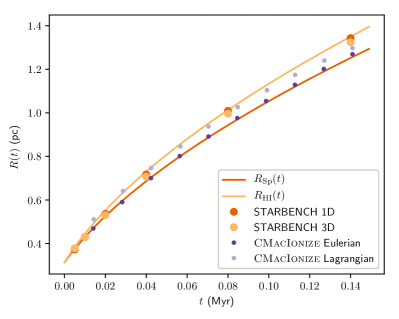
Figure 8: Position of the ionization front as a function of time for the STARBENCH benchmark. The full orange lines show the reference evolution curves, the purple dots are the simulation results. The orange circles show the average 1D and 3D results from Bisbas et al. (2015b).

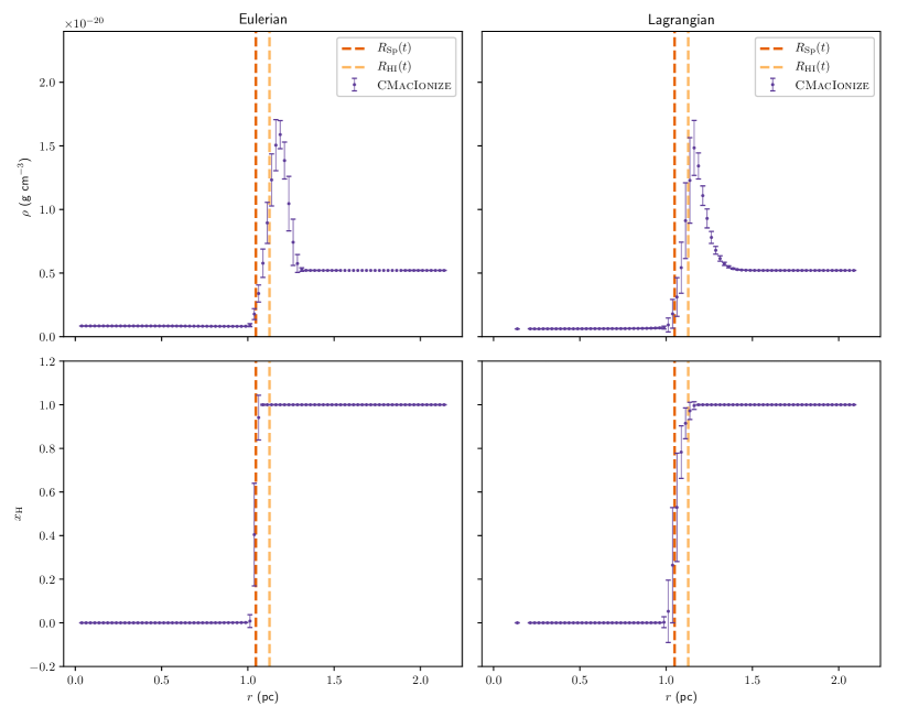
Figure 9: Density (top) and neutral fraction (bottom) as a function of radius for the STARBENCH benchmark test at $t=0.0987\leavevmode\nobreak\ \text{Myr}$. Left: Eulerian result, right: Lagrangian result. The orange dashed lines are the reference radii, the purple error bars are the simulation results.

This version corresponds to benchmark test starbench. It evolves the system forward in time using 2,048 fixed size time steps. The evolution of the ionization front is shown in Figure 8, and very closely follows the Spitzer solution (32). The left panels in Figure 9 show the density and neutral fraction as a function of radius for $t=0.0987\leavevmode\nobreak\ \text{Myr}$.

4.3.2 Lagrangian solution

This version corresponds to benchmark test starbench_voronoi. It evolves the system forward in time using only 256 fixed size time steps (since the average cell size is larger in this case). The evolution of the ionization front is again shown in Figure 8. This time, the ionization front first follows the Hosokawa-Inutsuka solution (33), and then slows down to the Spitzer solution (32). The density and neutral fraction profiles are shown in the right panels of Figure 9.

4.4 Parallel efficiency

As mentioned in 3.2.4, we have made most of our algorithm inherently parallel by designing it in terms of small tasks. In this subsection, we will illustrate how this affects the parallel scaling of the code. Since different modes of the code use different parts of the algorithm, we will rerun all of the benchmarks tests introduced above with different numbers of shared memory threads and distributed memory processes.

For all runs, we use a single node of our local high performance computing cluster Kennedy. This node has a 2.10 GHz Intel Xeon E5-2683 v4 processor with 16 physical cores, hyper-threaded to run 32 threads in parallel. Note that because of the hyper-threading, we do not expect perfect scaling if more than 16 cores are used, since then different threads will be competing for resources.

We will quantify the scaling through the speed up $S(n)$ of the algorithm as a function of the number of computing units $n$. It is given by

$$S(n)=\frac{t(1)}{t(n)},$$ (34)

where $t(n)$ is the total runtime of the algorithm when using $n$ computing units. For a hypothetical code that scales perfectly, the speed up is simply given by $S_{p}(n)=n$.

In practice, there are a number of important factors that can affect the parallel scaling, and cause $S(n)$ to lie below $S_{p}(n)$:

• The existence of serial parts of the code that are only executed by one computing unit while the other computing units are idle, or that are executed by all computing units (and hence duplicate work). These are located in parts of the algorithm that are not parallel. If $t_{s}(n)$ and $t_{p}(n)$ are respectively the runtime of the serial and the parallel part of the code when using $n$ computing units, then the theoretical maximum speed up is always lower than $S_{p}(n)$ (assuming $t_{p}(n)=\frac{t_{p}(1)}{n}$):

  $$S_{p,s}(n)=\left(\frac{t_{s}(1)+t_{p}(1)}{nt_{s}(1)+t_{p}(1)}\right)n.$$ (35)

• The overhead caused by running the algorithm in parallel. This overhead can be caused by extra code that needs to be executed as part of the parallelization strategy, or by delays caused by different computing units fighting over hardware access. Overhead will cause $t_{p,o}(n)>\frac{t_{p}(1)}{n}$, i.e. $t_{p,o}(n)=\frac{t_{p}(1)}{n}+t_{o}(n)$ (with $t_{o}(1)=0$). If the overhead is parallel, it is shared among the various computing units ($t_{o}(n)=\frac{t_{o,c}}{n}$). We can determine the constant from the 2 computing units measurement, and the speed up including overhead is

  $$S_{p,s+op}(n)=\left(\frac{t_{s}(1)+t_{p}(1)}{nt_{s}(1)+2t_{p,o}(2)}\right)n.$$ (36)

  If on the other hand the overhead is serial, it is constant per computing unit ($t_{o}(n)=t_{o,u}$), and the speed up is given by

  $$S_{p,s+os}(n)=\\ \left(\frac{t_{s}(1)+t_{p}(1)}{nt_{s}(1)+nt_{p,o}(2)+\left(1-\frac{n}{2}\right)t_{p}(1)}\right)n.$$ (37)

• The occurrence of load imbalances between different computing units that cause some computing units to sit idle while they are waiting for other computing units to finish a task. While load imbalances affect the scaling in the same way as serial parts of the code, we cannot directly measure them, and treat them in the same way as the overhead.

For this version of CMacIonize, we made the decision to only parallelize those parts of the algorithm that would lead to the most significant speed up, i.e. the photon traversal algorithm and the cell based computations. This means that there is still a significant fraction of serial code left in the algorithm, which we will address in future versions of the code. This will limit the expected scaling behaviour of the code, especially in simulations with small grid sizes and small photon packet numbers.

Since the serial version of the code uses the same task based strategy as the shared memory parallel version, the latter has no code based overhead (unless the code is configured without OpenMP, in which case the OpenMP calls will be absent). The only overhead will be caused by hardware concurrency issues: since different threads might attempt to write to the same grid cell during the photon traversal step, we need to lock each cell upon access. If another thread already obtained access to the cell, the thread trying to acquire the lock will sit idle until that cell becomes available, causing a small overhead.

The distributed memory parallel version of the code has a much larger code based overhead, as it requires communication between the different parallel processes which is completely absent from the serial version. The overhead is particularly large in our code, as we made the decision to store variables per cell rather than per variable type, which means we need to repack variables into separate communication buffers before we can send them to another process. We plan to address this issue as part of a future distributed memory parallel version that includes a domain decomposition to distribute the grid across multiple processes. We hence do not expect very good distributed memory scaling for our current version.

The task based shared memory parallelization strategy we use automatically takes care of the load balancing on a single node, as different threads get tasks from a shared task pool. The time a single thread will need to wait cannot be longer than the longest time it takes to finish a single task, so we can control the former by adapting the size of the latter. When a JobMarket (see 3.2.4) starts spawning tasks of a specific type, it usually starts with reasonably large task sizes, and then gradually makes the tasks smaller, until some lower limit is reached. This is illustrated in Figure 12. Using large initial task sizes limits the overhead caused by calls to the JobMarket, while the lower size limit sets the maximum load imbalance between different threads.

We do not perform any specific load balancing between distributed memory parallel processes, and simply try to assign equal photon numbers and cell numbers to each process when executing a step in parallel. A better load balancing scheme will be part of the future domain decomposed distributed memory algorithm.

Below, we will give the scaling results for the various benchmark tests. We will focus on shared memory parallelization for all tests, and only show distributed memory parallelization scaling for the Strömgren benchmark, as we still plan to change our distributed memory parallelization strategy in future versions of the code.

4.4.1 Photoionization only

Shared memory scaling

Table 5: Timing information for the shared memory scaling run of the Strömgren benchmark test (without diffuse field) on a system with 32 available cores.

$n$	$t(n)$ (s)	$t_{s}(n)$ (s)	$t_{o}(n)$ (s)
1	158.457	1.764	0.000
2	107.071	1.674	26.961
3	70.670	1.577	16.675
4	56.178	1.644	15.241
5	44.539	1.726	11.437
6	37.249	1.683	9.370
7	33.128	1.623	8.980
8	29.450	2.032	8.100
9	26.531	1.628	7.357
10	25.540	1.743	8.107
11	22.625	1.817	6.616
12	20.642	1.676	5.821
13	19.453	1.679	5.636
14	18.350	1.732	5.394
15	17.511	1.718	5.301
16	16.526	1.674	4.969
17	15.924	1.768	4.943
18	15.074	1.740	4.605
19	14.758	1.783	4.747
20	14.081	1.758	4.483
21	13.663	1.696	4.438
22	13.197	1.606	4.311
23	12.743	1.555	4.167
24	12.644	1.684	4.351
25	12.328	1.639	4.297
26	12.274	1.662	4.484
27	12.241	1.691	4.674
28	12.066	1.701	4.706
29	12.042	1.702	4.875
30	12.336	1.814	5.349
31	12.319	1.697	5.501
32	12.592	2.006	5.932

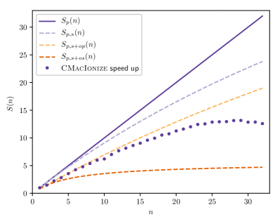
Figure 10: Speed up as a function of number of shared memory parallel threads for the Strömgren benchmark test (without diffuse field). The full purple line shows the theoretical perfect speed up, the dashed purple line is the perfect speed up taking into account the serial part of the code, as measured from the 1 thread run. The purple dots are the actual code results. In orange we show the speed up curves for parallel and serial overhead as estimated from the 2 thread run.

Table 5 and Figure 10 show the shared memory scaling measurements for the default version of the Strömgren benchmark test (without diffuse field). It is immediately obvious that there is a large overhead in the parallel runs. Comparing the speed up with the two speed up curves including overhead, we conclude that this overhead is parallel, and hence shared among the threads.

The most likely cause of the constant overhead is the locking mechanism, since the number of times a lock is used depends on the number of visited cells and is hence constant for a given simulation. In the serial run, no locks need to be set, and there is almost no overhead when locking and unlocking a cell. As soon as more than 1 thread is used, locking is necessary and the constant overhead will be added to the simulation time.

If we compare the scaling to $S_{p,s+op}(n)$, the parallel overhead scaling curve, we see good scaling up to 20 threads. After that, scaling decreases significantly. This is expected, as the 32 threads have to compete for the 16 available physical cores.

Distributed memory scaling

Table 6: Timing information for the distributed memory scaling run of the Strömgren benchmark test (without diffuse field) on a system with 32 available cores.

$n$	$t(n)$ (s)	$t_{s}(n)$ (s)	$t_{o}(n)$ (s)
1	160.613	1.708	0.000
2	108.900	2.192	27.740
3	86.124	1.744	31.448
4	73.623	1.657	32.189
5	66.784	1.732	33.295
6	62.263	1.841	34.071
7	60.972	2.580	36.563
8	56.100	2.048	34.529
9	55.613	2.133	36.249
10	54.367	2.665	36.769
11	56.128	2.949	39.974
12	52.518	3.297	37.568
13	54.639	1.970	40.708
14	53.979	4.033	40.921
15	51.954	3.197	39.653
16	50.357	2.745	38.718
17	50.973	2.532	39.918
18	49.690	2.353	39.154
19	49.313	2.177	39.242
20	49.338	2.310	39.685
21	48.730	3.318	39.455
22	48.250	3.046	39.319
23	46.816	2.259	38.199
24	47.624	2.747	39.295
25	47.438	2.419	39.374
26	47.331	3.552	39.511
27	46.753	2.846	39.160
28	45.965	2.721	38.582
29	45.232	2.563	38.045
30	46.483	2.605	39.478
31	44.717	2.662	37.883
32	44.706	3.822	38.032

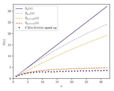
Figure 11: Speed up as a function of number of distributed memory parallel processes for the Strömgren benchmark test (without diffuse field). The full purple line shows the theoretical perfect speed up, the dashed purple line is the perfect speed up taking into account the serial part of the code, as measured from the 1 process run. The purple dots are the actual code results. In orange we show the speed up curves for parallel and serial overhead as estimated from the 2 processes run.

Table 6 and Figure 11 show the distributed memory scaling measurements for the default version of the Strömgren benchmark test (without diffuse field). Again there is a large overhead, but this time it is a serial overhead that is almost constant per process. This overhead is due to the repacking and communication, and due to load imbalances. Although there is a speed up and hence some gain from using multiple processes, the parallel scaling is poor.

Time line

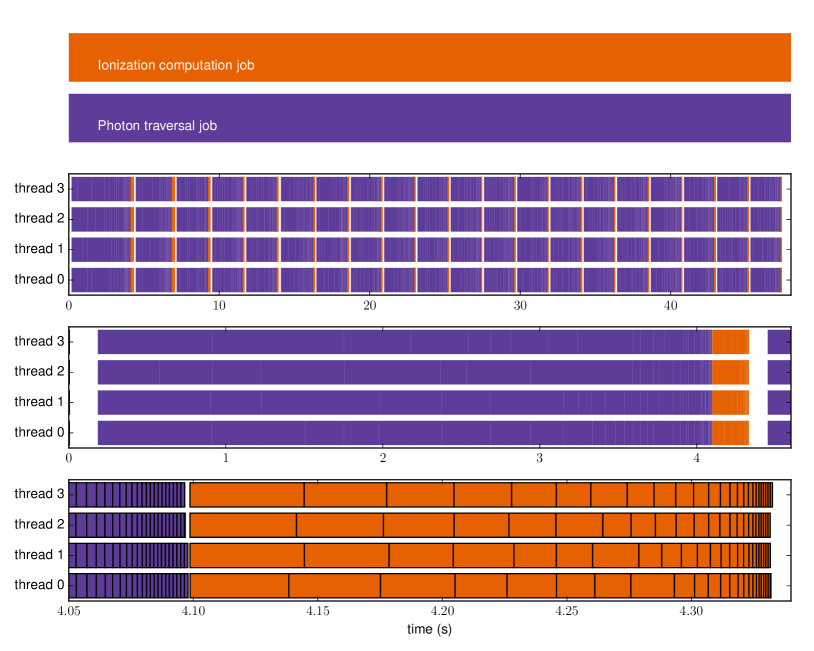
Figure 12: Time line of a shared memory parallel run, showing the various tasks being executed by different threads. Top: total time line, middle: zoom on the first photoionization iteration, showing the large serial part at the start of the simulation and in between subsequent iterations, bottom: zoom on the end of the first iteration, showing the small load imbalance between the various threads at the end of the different task categories.

Figure 12 shows a time line of the Strömgren benchmark test, run on 4 shared memory threads on the same node. The different coloured bars represent different tasks being executed, while the whitespace represents serial parts of the code, or parts where the threads are effectively waiting until all threads finished a specific type of jobs. Overall, the task based parallelism works well to reduce load imbalances between different threads. However, there are still some serial parts of the code that limit the scalability. This graph also does not show the time threads spend waiting to acquire locked resources, which can affect the summed total runtime of the photon traversal task.

4.4.2 Cooling and heating

Table 7: Timing information for the shared memory scaling run of the high temperature Lextington benchmark test on a system with 32 available cores.

$n$	$t(n)$ (s)	$t_{s}(n)$ (s)	$t_{o}(n)$ (s)
1	383.991	2.050	0.000
2	206.586	1.694	13.566
3	137.661	1.552	8.297
4	105.118	1.635	7.583
5	83.918	1.710	5.480
6	70.396	1.666	4.689
7	60.710	1.674	4.097
8	53.373	1.716	3.580
9	47.803	1.756	3.315
10	43.367	1.830	3.123
11	39.631	1.819	2.859
12	36.558	1.775	2.680
13	33.864	1.753	2.434
14	31.836	1.678	2.505
15	29.818	1.722	2.305
16	28.278	1.772	2.357
17	26.602	1.813	2.085
18	25.422	1.976	2.153
19	24.243	1.863	2.091
20	23.183	1.900	2.036
21	22.158	1.745	1.920
22	21.354	1.766	1.943
23	20.804	1.693	2.148
24	20.312	1.645	2.348
25	19.954	1.737	2.626
26	19.630	1.726	2.890
27	19.125	1.598	2.929
28	18.883	1.711	3.192
29	18.620	1.752	3.400
30	18.380	1.778	3.599
31	18.363	2.031	3.992
32	18.503	1.792	4.517

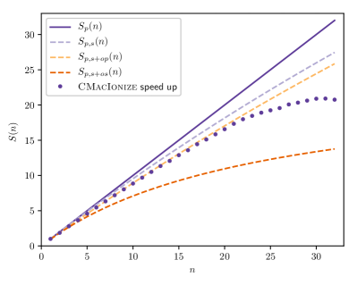
Figure 13: Speed up as a function of number of shared memory parallel threads for the high temperature Lexington benchmark. The full purple line shows the theoretical perfect speed up, the dashed purple line is the perfect speed up taking into account the serial part of the code, as measured from the 1 thread run. The purple dots are the actual code results. In orange we show the speed up curves for parallel and serial overhead as estimated from the 2 thread run.

Table 7 and Figure 13 show the shared memory scaling measurements for the default high temperature Lexington benchmark test. As in the Strömgren run, there is a considerable overhead due to the locking mechanism, but since we do a lot more work, this overhead is less noticeable. Overall, the code scales well up to 20 threads.

4.4.3 Radiation hydrodynamics

Table 8: Timing information for the shared memory scaling run of the STARBENCH benchmark test on a system with 32 available cores.

$n$	$t(n)$ (s)	$t_{s}(n)$ (s)	$t_{o}(n)$ (s)
1	266.779	7.688	0.000
2	180.832	6.798	43.598
3	127.426	7.062	33.374
4	103.211	6.752	30.750
5	86.684	6.761	27.178
6	77.835	6.742	26.965
7	70.042	7.042	25.341
8	63.489	6.756	23.415
9	61.477	7.031	25.001
10	61.021	6.711	27.424
11	59.448	6.948	28.206
12	58.676	6.677	29.397
13	58.356	7.043	30.738
14	58.028	6.808	31.833
15	58.679	6.795	33.719
16	57.233	6.716	33.352
17	57.437	6.774	34.508
18	57.136	7.279	35.054
19	59.106	6.672	37.782
20	57.044	6.697	36.402
21	56.868	6.768	36.843
22	57.060	6.920	37.595
23	58.660	7.086	39.707
24	59.691	6.924	41.207
25	56.175	6.936	38.124
26	58.387	6.700	40.734
27	57.452	6.989	40.168
28	58.521	6.748	41.580
29	59.500	6.834	42.878
30	59.405	7.067	43.080
31	58.506	7.201	42.460
32	59.636	7.227	43.851

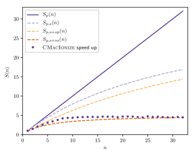
Figure 14: Speed up as a function of number of shared memory parallel threads for the STARBENCH benchmark. The full purple line shows the theoretical perfect speed up, the dashed purple line is the perfect speed up taking into account the serial part of the code, as measured from the 1 thread run. The purple dots are the actual code results. In orange we show the speed up curves for parallel and serial overhead as estimated from the 2 thread run.

Table 8 and Figure 14 show the shared memory scaling measurements for a short (10 time step) version of the default STARBENCH benchmark test. In this case, there is a significant serial fraction, and a considerable amount of overhead as well. The overhead is parallel at first, but switches to serial for high thread number. This is likely due to hardware issues, as the hydrodynamical integration scheme is more computation bound, and hence does not benefit from core hyper threading. Overall, there is still a lot of room for improvement of the scalability.

5 Conclusion

We presented the public Monte Carlo photoionization and moving-mesh RHD code CMacIonize, highlighted the implemented physics, and the most important design considerations during code development. We illustrated the usage and performance of the code with a number of relevant benchmark tests, and showed that it produces accurate and reproducable scientific results.

This work accompanies the first official release of the code (CMacIonize 1.0), and describes the code as it is for this version. A number of important improvements to the code are already on the way:

• implementation of a second order hydrodynamics solver,

• implementation of a distributed memory domain decomposition, using a scheme similar to Harries (2015), which would enable us to overcome current memory limitations that make it impossible to run large grids,

• optimization and full implementation of an alternative Voronoi grid construction algorithm (Vandenbroucke et al., in prep.), and

• implementation of more extensive atomic data using the Stout database (Lykins et al., 2015).

These will be part of future code releases.

References

Appendix A Fitting parameters for metal line cooling velocity-averaged collision strengths

Below we list the fit parameters to the collision strength data for all elements with low lying excited levels that are used in the code, grouped together per element and per ion of that element. The figures show the data points that were used in the fit, the actual fitting curve (with the same parameter precision as displayed in the tables), and the relative difference between the data values and the fitting curve, given by

$$\xi{}_{i\rightarrow{}j}(T)=\frac{\left|d(i\rightarrow{}j,T)-f(i\rightarrow{}j,T)\right|}{d(i\rightarrow{}j,T)+f(i\rightarrow{}j,T)},$$ (38)

where $d(i\rightarrow{}j,T)$ and $f(i\rightarrow{}j,T)$ are the data value and fit at temperature $T$ for the transition from level $i$ to level $j$ respectively.

Table 9: Fit parameters for the velocity-averaged collision strength data for carbon used in the code.

ion		$0\rightarrow{}1$	$0\rightarrow{}2$	$0\rightarrow{}3$	$0\rightarrow{}4$	$1\rightarrow{}2$
		$1\rightarrow{}3$	$1\rightarrow{}4$	$2\rightarrow{}3$	$2\rightarrow{}4$	$3\rightarrow{}4$
C+	$\begin{matrix}a\\ b\\ c\\ d\\ e\\ f\\ g\\ \end{matrix}$	-9.519e-01 -5.097e+00 1.436e+03 7.424e-01 -5.391e+01 3.673e-06 2.806e-07	1.247e-01 -2.710e-05 1.110e-01 2.784e-06 1.410e-02 -3.198e-08 -2.437e-09	3.496e-07 -2.076e-05 3.990e-01 2.426e-06 -2.832e+00 2.765e-10 2.159e-11	-2.814e-06 -2.407e-05 2.474e-01 2.906e-06 1.393e+00 -6.962e-10 -5.438e-11	1.949e-01 -9.811e-06 4.074e-02 1.003e-06 7.165e-03 -2.276e-08 -1.738e-09
	$\begin{matrix}a\\ b\\ c\\ d\\ e\\ f\\ g\\ \end{matrix}$	1.449e-01 -3.673e-05 1.713e-01 3.763e-06 -9.812e-03 6.304e-08 4.812e-09	-2.743e-06 -1.291e-04 1.183e+00 1.437e-05 1.598e+00 -2.263e-09 -1.753e-10	-1.195e-03 -2.027e-04 6.479e-01 2.660e-05 -7.636e-01 1.257e-08 9.795e-10	-4.787e-01 -1.490e-03 1.501e+01 9.750e-04 3.103e+00 -2.437e-07 -1.908e-08	-2.430e-03 -3.839e-04 1.605e+00 5.173e-05 -2.446e-01 8.372e-08 6.553e-09
C++	$\begin{matrix}a\\ b\\ c\\ d\\ e\\ f\\ g\\ \end{matrix}$	1.265e-07 5.762e-06 1.080e-01 -5.626e-07 1.412e+00 1.950e-11 1.323e-12	3.793e-07 1.727e-05 3.239e-01 -1.686e-06 1.095e+00 7.533e-11 5.111e-12	3.942e-07 2.877e-05 5.399e-01 -2.809e-06 6.095e-01 2.255e-10 1.530e-11	8.424e-06 7.004e-05 3.767e+00 -5.480e-06 -4.018e-01 -4.228e-10 -2.906e-11	5.033e-06 1.611e-04 6.600e-01 -1.477e-05 3.546e+00 1.577e-10 1.063e-11
	$\begin{matrix}a\\ b\\ c\\ d\\ e\\ f\\ g\\ \end{matrix}$	-6.251e-05 3.034e-04 1.039e-01 -2.744e-05 2.856e-01 3.444e-09 2.317e-10	1.741e-06 -1.148e-05 4.633e-01 7.853e-07 -4.244e+00 -5.205e-12 -3.781e-13	1.932e-05 8.772e-04 1.032e+00 -7.960e-05 3.735e+00 7.737e-10 5.206e-11	3.777e-04 -3.470e-05 1.386e+00 2.382e-06 4.838e-02 1.336e-09 9.718e-11	7.721e-06 -5.752e-05 2.317e+00 3.938e-06 5.449e-01 2.013e-10 1.463e-11

Table 10: Fit parameters for the velocity-averaged collision strength data for nitrogen used in the code.

ion		$0\rightarrow{}1$	$0\rightarrow{}2$	$0\rightarrow{}3$	$0\rightarrow{}4$	$1\rightarrow{}2$
		$1\rightarrow{}3$	$1\rightarrow{}4$	$2\rightarrow{}3$	$2\rightarrow{}4$	$3\rightarrow{}4$
N0	$\begin{matrix}a\\ b\\ c\\ d\\ e\\ f\\ g\\ \end{matrix}$	4.350e-04 -4.500e-04 2.206e-01 4.958e-05 7.786e-02 -1.099e-07 -8.271e-09	2.751e-06 -3.007e-04 1.474e-01 3.312e-05 3.882e-01 -1.470e-08 -1.106e-09	2.254e-07 -3.336e-05 2.277e-02 3.636e-06 8.211e-02 -5.171e-09 -3.695e-10	6.567e-06 -6.814e-05 4.632e-02 7.429e-06 5.470e-02 -1.612e-08 -1.155e-09	7.907e-02 -8.603e-03 6.355e+00 9.366e-04 1.259e-01 -1.315e-06 -9.950e-08
	$\begin{matrix}a\\ b\\ c\\ d\\ e\\ f\\ g\\ \end{matrix}$	-1.420e-02 -8.743e-03 3.581e+00 9.893e-04 8.734e-01 -2.580e-07 -1.983e-08	-3.258e-01 -1.290e+00 5.455e+02 1.451e-01 -1.122e+01 2.792e-06 2.138e-07	-3.592e-01 -9.058e-01 3.817e+02 1.019e-01 -1.055e+01 2.096e-06 1.606e-07	-1.910e-01 -9.570e-02 4.070e+01 1.077e-02 -5.010e+00 4.665e-07 3.574e-08	-2.313e-03 -2.099e-02 1.122e+01 2.337e-03 2.240e+00 -2.197e-07 -1.682e-08
N+	$\begin{matrix}a\\ b\\ c\\ d\\ e\\ f\\ g\\ \end{matrix}$	-3.483e-01 4.384e-03 2.059e+00 -4.032e-04 -3.391e-05 -1.192e-03 -8.966e-05	-2.779e-03 -2.640e-06 2.127e-01 1.368e-06 -7.504e-04 1.570e-06 1.229e-07	-1.472e-02 2.665e-05 2.965e-01 -2.560e-06 1.796e-07 1.600e-03 1.209e-04	2.426e-03 -1.170e-07 3.066e-02 2.803e-08 2.259e-09 -2.924e-03 -2.031e-04	-1.015e-01 6.264e-04 1.559e+00 -5.445e-05 1.428e-06 5.929e-04 3.183e-05
	$\begin{matrix}a\\ b\\ c\\ d\\ e\\ f\\ g\\ \end{matrix}$	-1.472e-02 7.995e-05 8.894e-01 -7.680e-06 5.191e-07 1.661e-03 1.255e-04	2.426e-03 -3.510e-07 9.197e-02 8.408e-08 7.197e-09 -2.753e-03 -1.912e-04	-1.473e-02 1.333e-04 1.482e+00 -1.280e-05 -1.036e-06 -1.390e-03 -1.048e-04	2.425e-03 -5.846e-07 1.533e-01 1.401e-07 -1.952e-07 1.690e-04 1.175e-05	2.226e-02 -3.918e-04 1.121e+00 3.934e-05 6.245e-06 -7.473e-04 -5.553e-05
N++	$\begin{matrix}a\\ b\\ c\\ d\\ e\\ f\\ g\\ \end{matrix}$	-3.257e-02 -3.573e-04 1.653e+00 4.822e-05 -7.529e-06 3.018e-03 2.453e-04

Table 11: Fit parameters for the velocity-averaged collision strength data for oxygen used in the code.

ion		$0\rightarrow{}1$	$0\rightarrow{}2$	$0\rightarrow{}3$	$0\rightarrow{}4$	$1\rightarrow{}2$
		$1\rightarrow{}3$	$1\rightarrow{}4$	$2\rightarrow{}3$	$2\rightarrow{}4$	$3\rightarrow{}4$
O0	$\begin{matrix}a\\ b\\ c\\ d\\ e\\ f\\ g\\ \end{matrix}$	-8.839e-01 -6.783e-03 7.448e-02 1.578e-03 3.239e-01 -2.549e-05 -3.727e-06	-7.697e-01 -9.788e-04 1.200e-02 2.477e-04 9.490e-01 -4.462e-07 -7.755e-08	-1.093e+00 1.413e+00 -1.373e+02 -1.998e-01 9.365e+00 3.197e-05 2.514e-06	-1.219e+00 6.529e-01 -5.311e+01 -9.393e-02 4.506e+00 2.706e-05 2.088e-06	-1.016e+00 -6.509e-03 6.884e-02 1.457e-03 1.015e+00 -1.947e-05 -2.390e-06
	$\begin{matrix}a\\ b\\ c\\ d\\ e\\ f\\ g\\ \end{matrix}$	-1.093e+00 8.480e-01 -8.239e+01 -1.199e-01 3.496e+00 5.140e-05 4.042e-06	-1.219e+00 3.917e-01 -3.187e+01 -5.636e-02 3.302e+00 2.216e-05 1.709e-06	-1.093e+00 2.827e-01 -2.746e+01 -3.996e-02 2.681e+00 2.234e-05 1.757e-06	-1.219e+00 1.306e-01 -1.062e+01 -1.879e-02 1.964e+00 1.242e-05 9.578e-07	-1.056e+00 -3.587e-01 3.534e+01 4.778e-02 1.295e+00 1.089e-05 6.545e-07
O+	$\begin{matrix}a\\ b\\ c\\ d\\ e\\ f\\ g\\ \end{matrix}$	-2.523e-03 -6.241e-06 8.502e-01 7.233e-07 1.444e-03 9.709e-09 1.522e-09	-1.125e-02 -8.446e-07 6.036e-01 2.181e-07 -1.635e-04 4.311e-08 -2.238e-10	1.161e-02 -4.213e-06 2.279e-01 4.878e-07 -1.033e-11 1.000e+00 2.265e+00	7.789e-02 -1.026e-05 7.464e-02 1.046e-06 1.431e-07 -8.913e-04 -6.598e-05	-8.588e-01 -4.648e+00 -3.736e+02 -1.190e+00 -1.466e-06 -5.766e+06 -9.308e-01
	$\begin{matrix}a\\ b\\ c\\ d\\ e\\ f\\ g\\ \end{matrix}$	-1.028e-02 -7.342e-05 8.844e-01 9.292e-06 -3.079e-04 7.387e-06 5.594e-07	-5.239e-02 -6.736e-06 4.666e-01 1.976e-06 -8.040e-04 1.289e-06 9.867e-08	-3.494e-02 -2.313e-05 5.770e-01 3.760e-06 -1.210e-03 1.098e-06 8.364e-08	1.038e-02 -3.425e-05 2.996e-01 4.003e-06 -2.143e-04 3.819e-06 2.881e-07	6.465e-02 -3.643e-05 1.838e-01 3.856e-06 -1.932e-07 2.875e-03 2.147e-04
O++	$\begin{matrix}a\\ b\\ c\\ d\\ e\\ f\\ g\\ \end{matrix}$	-2.517e-01 2.326e-03 2.174e+00 -2.246e-04 -4.349e-03 -5.803e-06 -4.351e-07	-2.886e-01 1.462e-03 1.373e+00 -1.364e-04 6.062e-03 2.338e-06 1.764e-07	-7.878e-01 -3.075e-02 5.015e+01 7.448e-03 -3.189e-03 6.917e-04 5.198e-05	-5.259e-01 1.618e-04 1.045e+00 2.345e-05 -7.038e-04 3.326e-05 2.552e-06	-2.714e-01 6.306e-03 5.834e+00 -5.990e-04 -5.646e-03 -1.140e-05 -8.562e-07
	$\begin{matrix}a\\ b\\ c\\ d\\ e\\ f\\ g\\ \end{matrix}$	-7.879e-01 -9.239e-02 1.505e+02 2.237e-02 1.919e-02 -3.453e-04 -2.593e-05	-5.259e-01 4.853e-04 3.136e+00 7.039e-05 -1.210e-03 5.806e-05 4.455e-06	-7.879e-01 -1.541e-01 2.510e+02 3.730e-02 6.860e-02 -1.610e-04 -1.209e-05	-5.260e-01 8.087e-04 5.229e+00 1.175e-04 -1.729e-03 6.777e-05 5.200e-06	6.242e-02 1.702e-04 1.766e-01 -1.776e-05 -2.314e-03 -1.121e-06 -8.415e-08

Table 12: Fit parameters for the velocity-averaged collision strength data for neon used in the code.

ion		$0\rightarrow{}1$	$0\rightarrow{}2$	$0\rightarrow{}3$	$0\rightarrow{}4$	$1\rightarrow{}2$
		$1\rightarrow{}3$	$1\rightarrow{}4$	$2\rightarrow{}3$	$2\rightarrow{}4$	$3\rightarrow{}4$
Ne+	$\begin{matrix}a\\ b\\ c\\ d\\ e\\ f\\ g\\ \end{matrix}$	-8.548e-01 1.938e-01 -1.038e+01 -1.254e-02 2.715e-02 5.755e-05 4.171e-06
Ne++	$\begin{matrix}a\\ b\\ c\\ d\\ e\\ f\\ g\\ \end{matrix}$	-6.515e-01 1.958e-01 -3.645e+01 -1.812e-02 -1.815e-03 -1.043e-03 -7.735e-05	-7.577e-01 1.184e-01 -2.862e+01 -1.047e-02 -9.100e-04 -1.094e-03 -8.029e-05	-5.448e-03 -9.752e-06 8.134e-01 7.937e-07 4.823e-06 3.627e-05 3.005e-06	1.019e-01 -8.068e-06 4.190e-02 8.074e-07 1.758e-08 -5.000e-03 -3.672e-04	-6.173e-01 4.546e-02 -8.088e+00 -4.215e-03 -2.781e-04 -1.537e-03 -1.139e-04
	$\begin{matrix}a\\ b\\ c\\ d\\ e\\ f\\ g\\ \end{matrix}$	-1.932e-03 -8.154e-06 4.758e-01 7.006e-07 -9.413e-05 -8.679e-07 -7.422e-08	1.161e-01 -5.770e-06 2.333e-02 5.826e-07 -6.898e-04 1.004e-07 7.445e-09	-2.118e-02 7.071e-06 1.788e-01 -7.768e-07 1.263e-07 1.534e-03 1.191e-04	9.843e-02 -1.648e-06 8.827e-03 1.628e-07 1.792e-08 -8.454e-04 -6.126e-05	5.812e-02 -4.021e-05 1.876e-01 4.268e-06 3.941e-03 -1.725e-07 -1.298e-08

Table 13: Fit parameters for the velocity-averaged collision strength data for sulphur used in the code.

ion		$0\rightarrow{}1$	$0\rightarrow{}2$	$0\rightarrow{}3$	$0\rightarrow{}4$	$1\rightarrow{}2$
		$1\rightarrow{}3$	$1\rightarrow{}4$	$2\rightarrow{}3$	$2\rightarrow{}4$	$3\rightarrow{}4$
S+	$\begin{matrix}a\\ b\\ c\\ d\\ e\\ f\\ g\\ \end{matrix}$	-2.378e-02 -3.780e-05 3.350e+00 2.326e-06 0.000e+00 0.000e+00 0.000e+00	-2.591e-02 -5.072e-05 5.088e+00 3.003e-06 0.000e+00 0.000e+00 0.000e+00	-4.744e-01 1.594e-02 1.361e+01 -1.274e-03 0.000e+00 0.000e+00 0.000e+00	-4.730e-01 3.177e-02 2.699e+01 -2.544e-03 0.000e+00 0.000e+00 0.000e+00	-8.272e-02 3.140e-05 1.492e+01 -5.602e-06 0.000e+00 0.000e+00 0.000e+00
	$\begin{matrix}a\\ b\\ c\\ d\\ e\\ f\\ g\\ \end{matrix}$	-5.368e-02 8.155e-05 2.216e+00 -6.673e-06 0.000e+00 0.000e+00 0.000e+00	-2.183e-02 5.571e-05 2.822e+00 -4.915e-06 0.000e+00 0.000e+00 0.000e+00	-1.569e-02 2.911e-05 2.012e+00 -2.687e-06 0.000e+00 0.000e+00 0.000e+00	-3.268e-02 1.339e-04 5.190e+00 -1.130e-05 0.000e+00 0.000e+00 0.000e+00	-5.249e-01 6.595e-02 4.606e+01 -5.206e-03 0.000e+00 0.000e+00 0.000e+00
S++	$\begin{matrix}a\\ b\\ c\\ d\\ e\\ f\\ g\\ \end{matrix}$	8.018e-02 -4.930e-05 1.206e+00 3.800e-06 0.000e+00 0.000e+00 0.000e+00	-2.250e-01 1.746e-03 3.814e+00 -1.408e-04 0.000e+00 0.000e+00 0.000e+00	-3.470e-02 6.561e-05 8.851e-01 -5.617e-06 0.000e+00 0.000e+00 0.000e+00	1.134e-01 3.383e-06 3.649e-02 -2.851e-07 0.000e+00 0.000e+00 0.000e+00	-4.587e-03 2.257e-04 4.846e+00 -1.949e-05 0.000e+00 0.000e+00 0.000e+00
	$\begin{matrix}a\\ b\\ c\\ d\\ e\\ f\\ g\\ \end{matrix}$	-4.454e-02 2.365e-04 2.823e+00 -2.014e-05 0.000e+00 0.000e+00 0.000e+00	1.665e-01 2.041e-06 6.825e-02 -1.900e-07 0.000e+00 0.000e+00 0.000e+00	-3.303e-02 3.185e-04 4.890e+00 -2.742e-05 0.000e+00 0.000e+00 0.000e+00	1.765e-01 2.565e-06 1.041e-01 -2.451e-07 0.000e+00 0.000e+00 0.000e+00	-2.273e-01 3.338e-03 2.390e+00 -2.696e-04 0.000e+00 0.000e+00 0.000e+00
S+++	$\begin{matrix}a\\ b\\ c\\ d\\ e\\ f\\ g\\ \end{matrix}$	-9.667e-01 -1.721e+01 2.979e+03 2.954e+00 -1.593e+01 9.973e-05 8.092e-06

Figure 25: Fits for S⁺.

Figure 26: Fits for S⁺⁺.

Figure 27: Fits for S⁺⁺⁺.

References

- Abdel-Naby et al. (2012) Abdel-Naby, S. A., Nikolić, D., Gorczyca, T. W., Korista, K. T., Badnell, N. R., Jan. 2012. Dielectronic recombination data for dynamic finite-density plasmas. XIV. The aluminum isoelectronic sequence. Astron. Astrophys. 537, A40.
- Alvarez et al. (2009) Alvarez, M. A., Busha, M., Abel, T., Wechsler, R. H., Oct. 2009. Connecting Reionization to the Local Universe. Astrophys. J. L. 703, L167–L171.
- Arnaud and Rothenflug (1985) Arnaud, M., Rothenflug, R., Jun. 1985. An updated evaluation of recombination and ionization rates. Astron. Astrophys., Suppl. Ser. 60, 425–457.
- Baczynski et al. (2015) Baczynski, C., Glover, S. C. O., Klessen, R. S., Nov. 2015. Fervent: chemistry-coupled, ionizing and non-ionizing radiative feedback in hydrodynamical simulations. Mon. Not. R. Astron. Soc. 454, 380–411.
- Barnes et al. (2014) Barnes, J. E., Wood, K., Hill, A. S., Haffner, L. M., Jun. 2014. Photoionization and heating of a supernova-driven turbulent interstellar medium. Mon. Not. R. Astron. Soc. 440, 3027–3035.
- Becker et al. (2001) Becker, R. H., Fan, X., White, R. L., Strauss, M. A., Narayanan, V. K., Lupton, R. H., Gunn, J. E., Annis, J., Bahcall, N. A., Brinkmann, J., Connolly, A. J., Csabai, I., Czarapata, P. C., Doi, M., Heckman, T. M., Hennessy, G. S., Ivezić, Ž., Knapp, G. R., Lamb, D. Q., McKay, T. A., Munn, J. A., Nash, T., Nichol, R., Pier, J. R., Richards, G. T., Schneider, D. P., Stoughton, C., Szalay, A. S., Thakar, A. R., York, D. G., Dec. 2001. Evidence for Reionization at z~6: Detection of a Gunn-Peterson Trough in a z=6.28 Quasar. Astron. J. 122, 2850–2857.
- Benítez-Llambay et al. (2015) Benítez-Llambay, A., Navarro, J. F., Abadi, M. G., Gottlöber, S., Yepes, G., Hoffman, Y., Steinmetz, M., Jul. 2015. The imprint of reionization on the star formation histories of dwarf galaxies. Mon. Not. R. Astron. Soc. 450, 4207–4220.
- Berrington (1988) Berrington, K. A., 1988. Low-energy electron excitation of the 3P(e) fine-structure levels in atomic oxygen. Journal of Physics B Atomic Molecular Physics 21, 1083–1089.
- Berrington et al. (1985) Berrington, K. A., Burke, P. G., Dufton, P. L., Kingston, A. E., 1985. Electron-Impact-Excitation Collision Strengths for Be-like Ions. II. Intermediate-Energy Region and Collision Rates. Atomic Data and Nuclear Data Tables 33, 195.
- Bisbas et al. (2015a) Bisbas, T. G., Haworth, T. J., Barlow, M. J., Viti, S., Harries, T. J., Bell, T., Yates, J. A., Dec. 2015a. TORUS-3DPDR: a self-consistent code treating three-dimensional photoionization and photodissociation regions. Mon. Not. R. Astron. Soc. 454, 2828–2843.
- Bisbas et al. (2015b) Bisbas, T. G., Haworth, T. J., Williams, R. J. R., Mackey, J., Tremblin, P., Raga, A. C., Arthur, S. J., Baczynski, C., Dale, J. E., Frostholm, T., Geen, S., Haugbølle, T., Hubber, D., Iliev, I. T., Kuiper, R., Rosdahl, J., Sullivan, D., Walch, S., Wünsch, R., Oct. 2015b. STARBENCH: the D-type expansion of an H II region. Mon. Not. R. Astron. Soc. 453, 1324–1343.
- Bisbas et al. (2009) Bisbas, T. G., Wünsch, R., Whitworth, A. P., Hubber, D. A., Apr. 2009. Smoothed particle hydrodynamics simulations of expanding H II regions. I. Numerical method and applications. Astron. Astrophys. 497, 649–659.
- Black (1981) Black, J. H., Nov. 1981. The physical state of primordial intergalactic clouds. Mon. Not. R. Astron. Soc. 197, 553–563.
- Blum and Pradhan (1992) Blum, R. D., Pradhan, A. K., May 1992. Rate coefficients for the excitation of infrared and ultraviolet lines in C II, N III, and O IV. Astrophys. J., Suppl. Ser. 80, 425–452.
- Brown and Mathews (1970) Brown, R. L., Mathews, W. G., Jun. 1970. Theoretical Continuous Spectra of Gaseous Nebulae. Astrophys. J. 160, 939.
- Burgess and Tully (1992) Burgess, A., Tully, J. A., Feb. 1992. On the Analysis of Collision Strengths and Rate Coefficients. Astron. Astrophys. 254, 436.
- Butler and Zeippen (1994) Butler, K., Zeippen, C. J., Nov. 1994. Atomic data from the IRON Project. V. Effective collision strengths for transitions in the ground configuration of oxygen-like ions. Astron. Astrophys., Suppl. Ser. 108.
- Camps et al. (2013) Camps, P., Baes, M., Saftly, W., Dec. 2013. Using 3D Voronoi grids in radiative transfer simulations. Astron. Astrophys. 560, A35.
- De Rijcke et al. (2013) De Rijcke, S., Schroyen, J., Vandenbroucke, B., Jachowicz, N., Decroos, J., Cloet-Osselaer, A., Koleva, M., Aug. 2013. New composition-dependent cooling and heating curves for galaxy evolution simulations. Mon. Not. R. Astron. Soc. 433, 3005–3016.
- Ercolano et al. (2005) Ercolano, B., Barlow, M. J., Storey, P. J., Sep. 2005. The dusty MOCASSIN: fully self-consistent 3D photoionization and dust radiative transfer models. Mon. Not. R. Astron. Soc. 362, 1038–1046.
- Faucher-Giguère et al. (2009) Faucher-Giguère, C.-A., Lidz, A., Zaldarriaga, M., Hernquist, L., Oct. 2009. A New Calculation of the Ionizing Background Spectrum and the Effects of He II Reionization. Astrophys. J. 703, 1416–1443.
- Ferland (1995) Ferland, G., 1995. The Lexington Benchmarks for Numerical Simulations of Nebulae. In: Williams, R., Livio, M. (Eds.), The Analysis of Emission Lines: A Meeting in Honor of the 70th Birthdays of D. E. Osterbrock & M. J. Seaton. p. 83.
- Ferland et al. (2017) Ferland, G. J., Chatzikos, M., Guzmán, F., Lykins, M. L., van Hoof, P. A. M., Williams, R. J. R., Abel, N. P., Badnell, N. R., Keenan, F. P., Porter, R. L., Stancil, P. C., Oct. 2017. The 2017 Release Cloudy. Rev. Mex. Astron. Astroph. 53, 385–438.
- Froese Fischer and Tachiev (2004) Froese Fischer, C., Tachiev, G., May 2004. Breit-Pauli energy levels, lifetimes, and transition probabilities for the beryllium-like to neon-like sequences. Atomic Data and Nuclear Data Tables 87, 1–184.
- Galavis et al. (1997) Galavis, M. E., Mendoza, C., Zeippen, C. J., May 1997. Atomic data from the IRON Project. XXII. Radiative rates for forbidden transitions within the ground configuration of ions in the carbon and oxygen isoelectronic sequences. Astron. Astrophys., Suppl. Ser. 123.
- Galavis et al. (1998) Galavis, M. E., Mendoza, C., Zeippen, C. J., Sep. 1998. Atomic data from the IRON Project. XXIX. Radiative rates for transitions within the N = 2 complex in ions of the boron isoelectronic sequence. Astron. Astrophys., Suppl. Ser. 131, 499–522.
- Gamma et al. (1995) Gamma, E., Helm, R., Johnson, R., Vlissides, J., 1995. Design Patterns: Elements of Reusable Object-oriented Software. Addison-Wesley Longman Publishing Co., Inc., Boston, MA, USA.
- Griffin et al. (2001) Griffin, D. C., Mitnik, D. M., Badnell, N. R., Nov. 2001. Electron-impact excitation of Ne+. Journal of Physics B Atomic Molecular Physics 34, 4401–4415.
- Harries (2000) Harries, T. J., Jul. 2000. Synthetic line profiles of rotationally distorted hot-star winds. Mon. Not. R. Astron. Soc. 315, 722–734.
- Harries (2015) Harries, T. J., Apr. 2015. Radiation-hydrodynamical simulations of massive star formation using Monte Carlo radiative transfer - I. Algorithms and numerical methods. Mon. Not. R. Astron. Soc. 448, 3156–3166.
- Harries et al. (2017) Harries, T. J., Douglas, T. A., Ali, A., Nov. 2017. Radiation-hydrodynamical simulations of massive star formation using Monte Carlo radiative transfer - II. The formation of a 25 solar-mass star. Mon. Not. R. Astron. Soc. 471, 4111–4120.
- Hoffmann et al. (2003) Hoffmann, T. L., Pauldrach, A. W. A., Puls, J., 2003. Wind models and synthetic UV spectra for O-type stars. In: van der Hucht, K., Herrero, A., Esteban, C. (Eds.), A Massive Star Odyssey: From Main Sequence to Supernova. Vol. 212 of IAU Symposium. p. 206.
- Hopkins (2015) Hopkins, P. F., Jun. 2015. A new class of accurate, mesh-free hydrodynamic simulation methods. Mon. Not. R. Astron. Soc. 450, 53–110.
- Hosokawa and Inutsuka (2006) Hosokawa, T., Inutsuka, S.-i., Jul. 2006. Dynamical Expansion of Ionization and Dissociation Front around a Massive Star. II. On the Generality of Triggered Star Formation. Astrophys. J. 646, 240–257.
- Hudson et al. (2012) Hudson, C. E., Ramsbottom, C. A., Scott, M. P., May 2012. Collision Strengths and Effective Collision Strengths for Transitions within the Ground-state Configuration of S III. Astrophys. J. 750, 65.
- Katz et al. (1996) Katz, N., Weinberg, D. H., Hernquist, L., Jul. 1996. Cosmological Simulations with TreeSPH. Astrophys. J., Suppl. Ser. 105, 19.
- Kaufman and Sugar (1986) Kaufman, V., Sugar, J., Jan. 1986. Forbidden Lines in ns2npk Ground Configurations and nsnp Excited Configurations of Beryllium through Molybdenum Atoms and Ions. Journal of Physical and Chemical Reference Data 15, 321–426.
- Kingdon and Ferland (1996) Kingdon, J. B., Ferland, G. J., Sep. 1996. Rate Coefficients for Charge Transfer between Hydrogen and the First 30 Elements. Astrophys. J., Suppl. Ser. 106, 205.
- Kisielius et al. (2009) Kisielius, R., Storey, P. J., Ferland, G. J., Keenan, F. P., Aug. 2009. Electron-impact excitation of OII fine-structure levels. Mon. Not. R. Astron. Soc. 397, 903–912.
- Klassen et al. (2012) Klassen, M., Peters, T., Pudritz, R. E., Oct. 2012. H II Region Variability and Pre-main-sequence Evolution. Astrophys. J. 758, 137.
- Kolb et al. (2013) Kolb, S. M., Stute, M., Kley, W., Mignone, A., Nov. 2013. Radiation hydrodynamics integrated in the PLUTO code. Astron. Astrophys. 559, A80.
- Lennon and Burke (1994) Lennon, D. J., Burke, V. M., Feb. 1994. Atomic data from the IRON project. II. Effective collision strength S for infrared transitions in carbon-like ions. Astron. Astrophys., Suppl. Ser. 103.
- Lykins et al. (2015) Lykins, M. L., Ferland, G. J., Kisielius, R., Chatzikos, M., Porter, R. L., van Hoof, P. A. M., Williams, R. J. R., Keenan, F. P., Stancil, P. C., Jul. 2015. Stout: Cloudy’s Atomic and Molecular Database. Astrophys. J. 807, 118.
- Mackey et al. (2016) Mackey, J., Haworth, T. J., Gvaramadze, V. V., Mohamed, S., Langer, N., Harries, T. J., Feb. 2016. Detecting stellar-wind bubbles through infrared arcs in H II regions. Astron. Astroph. 586, A114.
- Martin et al. (1990) Martin, W. C., Zalubas, R., Musgrove, A., Jul. 1990. Energy Levels of Sulfur, S I Through S XVI. Journal of Physical and Chemical Reference Data 19, 821–880.
- Mazzotta et al. (1998) Mazzotta, P., Mazzitelli, G., Colafrancesco, S., Vittorio, N., Dec. 1998. Ionization balance for optically thin plasmas: Rate coefficients for all atoms and ions of the elements H to NI. Astron. Astrophys., Suppl. Ser. 133, 403–409.
- Mendoza and Zeippen (1982) Mendoza, C., Zeippen, C. J., Jun. 1982. Transition probabilities for forbidden lines in the 3p/2/ configuration. - II. Mon. Not. R. Astron. Soc. 199, 1025–1032.
- Nussbaumer and Storey (1983) Nussbaumer, H., Storey, P. J., Sep. 1983. Dielectronic recombination at low temperatures. Astron. Astrophys. 126, 75–79.
- Nussbaumer and Storey (1987) Nussbaumer, H., Storey, P. J., Apr. 1987. Dielectronic recombination at low temperatures. IV - Recombination coefficients for neon. Astron. Astrophys., Suppl. Ser. 69, 123–133.
- Osterbrock and Ferland (2006) Osterbrock, D. E., Ferland, G. J., 2006. Astrophysics of gaseous nebulae and active galactic nuclei.
- Pawlik and Schaye (2008) Pawlik, A. H., Schaye, J., Sep. 2008. TRAPHIC - radiative transfer for smoothed particle hydrodynamics simulations. Mon. Not. R. Astron. Soc. 389, 651–677.
- Péquignot et al. (2001) Péquignot, D., Ferland, G., Netzer, H., Kallman, T., Ballantyne, D. R., Dumont, A.-M., Ercolano, B., Harrington, P., Kraemer, S., Morisset, C., Nayakshin, S., Rubin, R. H., Sutherland, R., 2001. Photoionization Model Nebulae. In: Ferland, G., Savin, D. W. (Eds.), Spectroscopic Challenges of Photoionized Plasmas. Vol. 247 of Astronomical Society of the Pacific Conference Series. p. 533.
- Peters et al. (2017) Peters, T., Naab, T., Walch, S., Glover, S. C. O., Girichidis, P., Pellegrini, E., Klessen, R. S., Wünsch, R., Gatto, A., Baczynski, C., Apr. 2017. The SILCC project - IV. Impact of dissociating and ionizing radiation on the interstellar medium and H emission as a tracer of the star formation rate. Mon. Not. R. Astron. Soc. 466, 3293–3308.
- Pradhan (1995) Pradhan, A., 1995. Atomic Data for the Analysis of Emission Lines. In: Williams, R., Livio, M. (Eds.), The Analysis of Emission Lines: A Meeting in Honor of the 70th Birthdays of D. E. Osterbrock & M. J. Seaton. p. 8.
- Rosdahl et al. (2013) Rosdahl, J., Blaizot, J., Aubert, D., Stranex, T., Teyssier, R., Dec. 2013. RAMSES-RT: radiation hydrodynamics in the cosmological context. Mon. Not. R. Astron. Soc. 436, 2188–2231.
- Saftly et al. (2014) Saftly, W., Baes, M., Camps, P., Jan. 2014. Hierarchical octree and k-d tree grids for 3D radiative transfer simulations. Astron. Astrophys. 561, A77.
- Saraph and Storey (1999) Saraph, H. E., Storey, P. J., Jan. 1999. Atomic data from the IRON Project. XXX. Collision data for the (2) P^o_1over 2 - ^2P(o_3/) 2 fine-structure lines of P iii, S IV and CL V. Astron. Astroph., Suppl. Ser. 134, 369–375.
- Saraph and Tully (1994) Saraph, H. E., Tully, J. A., Oct. 1994. Atomic data from the IRON project. IV. Electron excitation of the ^2^P^0^_3/2_-^2^P^0^_1/2_ fine structure transition in fluorine-like ions. Astron. Astrophys., Suppl. Ser. 107.
- Spitzer (1978) Spitzer, L., 1978. Physical processes in the interstellar medium.
- Springel (2010) Springel, V., Jan. 2010. E pur si muove: Galilean-invariant cosmological hydrodynamical simulations on a moving mesh. Mon. Not. R. Astron. Soc. 401, 791–851.
- Steinacker et al. (2013) Steinacker, J., Baes, M., Gordon, K. D., Aug. 2013. Three-Dimensional Dust Radiative Transfer*. Ann. Rev. Astron. Astrophys. 51, 63–104.
- Storey and Hummer (1995) Storey, P. J., Hummer, D. G., Jan. 1995. Recombination line intensities for hydrogenic ions-IV. Total recombination coefficients and machine-readable tables for Z=1 to 8. Mon. Not. R. Astron. Soc. 272, 41–48.
- Strömgren (1939) Strömgren, B., May 1939. The Physical State of Interstellar Hydrogen. Astrophys. J. 89, 526.
- Tayal (2000) Tayal, S. S., Nov. 2000. Effective Collision Strengths for Electron Impact Excitation of N I. Atomic Data and Nuclear Data Tables 76, 191–212.
- Tayal (2008) Tayal, S. S., Aug. 2008. Electron impact excitation collision strength for transitions in C II. Astron. Astrophys. 486, 629–636.
- Tayal and Zatsarinny (2010) Tayal, S. S., Zatsarinny, O., May 2010. Breit-Pauli Transition Probabilities and Electron Excitation Collision Strengths for Singly Ionized Sulfur. Astrophys. J., Suppl. Ser. 188, 32–45.
- Toro (2009) Toro, E. F., 2009. Riemann Solvers and Numerical Methods for Fluid Dynamics, 3rd Edition. Springer-Verlag, Berlin Heidelberg.
- Vandenbroucke and De Rijcke (2016) Vandenbroucke, B., De Rijcke, S., Jul. 2016. The moving mesh code SHADOWFAX. Astron. Comput. 16, 109–130.
- Vandenbroucke et al. (2016) Vandenbroucke, B., Verbeke, R., De Rijcke, S., May 2016. Constraining the subgrid physics in simulations of isolated dwarf galaxies. Mon. Not. R. Astron. Soc. 458, 912–933.
- Vandenbroucke et al. (2018) Vandenbroucke, B., Wood, K., Girichidis, P., Hill, A., Peters, T., 2018. Radiative transfer calculations of the diffuse ionised gas in disc galaxies. submitted to Mon. Not. R. Astron. Soc.
- Verner and Ferland (1996) Verner, D. A., Ferland, G. J., Apr. 1996. Atomic Data for Astrophysics. I. Radiative Recombination Rates for H-like, He-like, Li-like, and Na-like Ions over a Broad Range of Temperature. Astrophys. J., Suppl. Ser. 103, 467.
- Verner et al. (1996) Verner, D. A., Ferland, G. J., Korista, K. T., Yakovlev, D. G., Jul. 1996. Atomic Data for Astrophysics. II. New Analytic FITS for Photoionization Cross Sections of Atoms and Ions. Astrophys. J. 465, 487.
- Wood et al. (2004) Wood, K., Mathis, J. S., Ercolano, B., Mar. 2004. A three-dimensional Monte Carlo photoionization code for modelling diffuse ionized gas. Mon. Not. R. Astron. Soc. 348, 1337–1347.
- Zatsarinny and Tayal (2003) Zatsarinny, O., Tayal, S. S., Oct. 2003. Electron Collisional Excitation Rates for O I Using the B-Spline R-Matrix Approach. Astrophys. J., Suppl. Ser. 148, 575–582.