Strategies for Reduced-Order Models for Predicting the Statistical Responses and Uncertainty Quantification in Complex Turbulent Dynamical Systems

Abstract

Turbulent dynamical systems characterized by both a high-dimensional phase space and a large number of instabilities are ubiquitous among many complex systems in science and engineering including climate, material, and neural science. The existence of a strange attractor in the turbulent systems containing a large number of positive Lyapunov exponents results in a rapid growth of small uncertainties from imperfect modeling equations or perturbations in initial values, requiring naturally a probabilistic characterization for the evolution of the turbulent system. Uncertainty quantification (UQ) in turbulent dynamical systems is a grand challenge where the goal is to obtain statistical estimates such as the change in mean and variance for key physical quantities in their nonlinear responses to changes in external forcing parameters or uncertain initial data. In the development of a proper UQ scheme for systems of high or infinite dimensionality with instabilities, significant model errors compared with the true natural signal are always unavoidable due to both the imperfect understanding of the underlying physical processes and the limited computational resources available through direct Monte-Carlo integration. One central issue in contemporary research is the development of a systematic methodology that can recover the crucial features of the natural system in statistical equilibrium (model fidelity) and improve the imperfect model prediction skill in response to various external perturbations (model sensitivity).

A general mathematical framework to construct statistically accurate reduced-order models that have skill in capturing the statistical variability in the principal directions with largest energy of a general class of damped and forced complex turbulent dynamical systems is discussed here. There are generally three stages in the modeling strategy, imperfect model selection; calibration of the imperfect model in a training phase; and prediction of the responses with UQ to a wide class of forcing and perturbation scenarios. The methods are developed under a universal class of turbulent dynamical systems with quadratic nonlinearity that is representative in many applications in applied mathematics and engineering. Several mathematical ideas will be introduced to improve the prediction skill of the imperfect reduced-order models. Most importantly, empirical information theory and statistical linear response theory are applied in the training phase for calibrating model errors to achieve optimal imperfect model parameters; and total statistical energy dynamics are introduced to improve the model sensitivity in the prediction phase especially when strong external perturbations are exerted. The validity of general framework of reduced-order models is demonstrated on instructive stochastic triad models. Recent applications to two-layer baroclinic turbulence in the atmosphere and ocean with combinations of turbulent jets and vortices are also surveyed. The uncertainty quantification and statistical response for these complex models are accurately captured by the reduced-order models with only $2\times 10^{2}$ modes in a highly turbulent system with $1\times 10^{5}$ degrees of freedom. Less than $0.15\%$ of the total spectral modes are needed in the reduced-order models.

76F55, 60H30, 86A32

Turbulent dynamical systems characterized by both a high-dimensional phase space and a large number of instabilities are ubiquitous among many complex systems in science and engineering [51, 54, 92, 75]. The existence of a strange attractor [93] in turbulent systems containing a large number of positive Lyapunov exponents results in a rapid growth of small uncertainties from imperfect modeling equations or perturbations in initial values, requiring naturally a probabilistic characterization for the evolution of the turbulent system. Uncertainty quantification (UQ) in turbulent dynamical systems is a grand challenge where the goal is to obtain statistical estimates such as the change in mean and variance for key physical quantities in their nonlinear responses to changes in external forcing parameters or uncertain initial data. One problem of practical significance in contemporary science is using UQ to understand the complexity of anisotropic turbulent processes over a wide range of spatio-temporal scales in engineering shear turbulence [35, 91, 26] as well as climate atmosphere ocean science [84, 92, 51]. This is especially important from a practical viewpoint because energy often flows intermittently from the smaller scales to affect the largest scales in such anisotropic turbulent flows.

In the development of a proper UQ scheme for systems of high or infinite dimensionality with instabilities, the analysis and prediction of phenomena often occur through complex dynamical equations that have significant model errors compared with the true natural signal. The imperfect model errors are always unavoidable due to both the imperfect understanding of the underlying physical processes and the limited computational resources needed for repeated Monte-Carlo simulations in each different scenario of high dimensional systems. Clearly, it is important both to improve the imperfect model’s capabilities to recover crucial features of the natural system and also to accurately model the sensitivities in the natural system to changes in external or internal parameters. These efforts are hampered by the fact that the actual dynamics of the natural system are unknown. Important examples with major societal impact involve the Earth’s climate and climate change where climate sensitivities are studied through a suite of imperfect comprehensive computer models ([22, 80, 57], and references therein); other examples include imperfect mesoscopic models in materials science [13, 39] and neural science [81] when compared with actual observed behavior in these complex nonlinear systems.

Recently, information theory has been utilized in different ways to systematically improve model fidelity and sensitivity [58, 57], to quantify the role of coarse-grained initial states in long-range forecasting [28, 29], and to make an empirical link between model fidelity and forecasting skill [19, 20]. Imperfect models for complex systems are constrained by their capability to reproduce certain statistics in a training phase where the natural system has been observed; for example, this training phase in climate science is roughly the 60-year dataset of extensive observations of the Earth’s climate system. For long-range forecasting, it is natural to guarantee statistical equilibrium fidelity for an imperfect model, and a framework using information theory is a natural way to achieve this in an unbiased fashion [58, 57, 28, 29, 20]. First, equilibrium statistical fidelity for an imperfect model depends on the choice of coarse-grained variables utilized [58, 57]; second, equilibrium model fidelity is a necessary but not sufficient condition to guarantee long-range forecasting skill [59, 29]. For example, Section 2.6 of [48] extensively discusses three very different strongly mixing chaotic dynamical models with 40 variables and with the same Gaussian equilibrium measure, the TBH, K-Z, and IL-96 models.

One significant application of UQ through empirical information theory is quantifying uncertainty in climate change science [57, 54]. The climate is an extremely complex coupled system involving multiple physical processes for the atmosphere, ocean, and land over a wide range of spatial scales from millimeters to thousands of kilometers and time scales from minutes to decades or centuries [22, 74]. Climate change science focuses on predicting the coarse-grained planetary scale long time changes in the climate system due to either changes in external forcing or internal variability such as the impact of increased carbon dioxide [31, 29]. For several decades the predictions of climate change science have been carried out with some skill through comprehensive computational atmospheric and oceanic simulation (AOS) models [22, 74, 80], which are designed to mimic the complex physical spatio-temporal patterns in nature. Such AOS models either through lack of resolution due to current computing power or through inadequate observation of nature necessarily parameterize the impact of many features of the climate system such as clouds, mesoscale and submesoscale ocean eddies, sea ice cover, etc. Thus, there are intrinsic model errors in the AOS models for the climate system and the effect of such model errors on predicting the coarse-grained large scale long time quantities is of interest. One central scientific issue in contemporary climate change science is the development of a systematic methodology that can recover the crucial features of the natural system in statistical equilibrium/climate (model fidelity) and improve the imperfect model prediction skill in response to various external perturbations like climate change and mitigation scenarios (model sensitivity) [2, 5, 20, 59, 54].

Here we discuss a general mathematical framework to construct statistically accurate reduced-order models that have the skill in capturing the statistical variability in the principal directions with largest energy of a general class of damped and forced complex turbulent dynamical systems. Low-order truncation methods is especially important for UQ with practical impact since the curse of ensemble size [6, 54] forbids to run Monte-Carlo simulations for all possible uncertain forcing scenarios in order to do attribution studies. Thus reduced-order models (ROM) are needed on a low-dimensional subspace where key physical significant quantities are characterized by the degrees of freedom that carry the largest energy or variance. In general, there are three stages in the modeling procedure, imperfect model selection; calibration of the imperfect model in a training phase using only data in the low-order perfect statistics; and prediction of the responses to a wide class of forcing and perturbation scenarios. The methods are developed for a universal class of turbulent dynamical systems with quadratic nonlinearity that is representative in many applications in applied mathematics and engineering [56, 51, 54]. Several mathematical ideas will be introduced to help improve the prediction skill of the imperfect reduced-order models. Most importantly, empirical information theory [48] and statistical linear response theory [59] are applied in the training phase for calibrating model errors to achieve optimal imperfect model parameters; and total statistical energy dynamics [53] are introduced to improve the model sensitivity in the prediction phase especially when strong external perturbations are exerted. The validity of general framework of reduced-order models has been verified by testing the methods on a series of representative turbulent dynamical models ranging from the 40-dimensional Lorenz ’96 model [63], one-layer barotropic turbulence with topography [78], and finally the two-layer baroclinic turbulence with internal instability [79].

In the following parts of the paper, we first display the general formulation of the turbulent system with quadratic nonlinearity, and its statistical moment dynamical equations in Section 1. The skill and limitation of many previous low-order modeling ideas are also discussed. Theoretical toolkits that are useful for the development of reduced-order models are introduced in Section 2, where a general strategy to improve imperfect model sensitivity is described using empirical information theory and a general total statistical energy dynamics. Section 3 discusses the construction of reduced-order models in detail under this general framework with these various theoretical tools. In Section 4, we illustrate all these procedures and algorithms for the reduced-order models for some simple but instructive systems of triad stochastic equations with several novel features. In Section 5, we give examples of the skill of the procedures and algorithms on two-layer baroclinic models for both atmosphere and ocean regimes with turbulent jets and vortices with roughly $1\times 10^{5}$ degrees of freedom and direct and inverse turbulent cascades. In these very tough regimes, the reduced-order strategies show skill in capturing the response to changes in external forcing using only $200$ modes, less than $0.15\%$ of the modes in the original system.

1 General Formulation of Turbulent Dynamical Systems with Nonlinearity

One representative feature in many turbulent dynamical systems from nature is the quadratic energy conserving nonlinear interaction that transfers energy from the unstable modes to stable ones where the energy is dissipated resulting in a statistical steady state in equilibrium. We consider the following abstract formulation of the turbulent dynamical systems about state variables $\mathbf{u}\in\mathbb{R}^{N}$ in a high-dimensional phase space

(1.1) $$\frac{d\mathbf{u}}{dt}=\left(\mathcal{L+D}\right)\mathbf{u}+B\left(\mathbf{u},\mathbf{u}\right)+\mathbf{F}\left(t\right)+\boldsymbol{\sigma}\left(t\right)\dot{\mathbf{W}}\left(t;\omega\right).$$

On the right hand side of the above equation (1.1), the first two components, $\left(\mathcal{L+D}\right)\mathbf{u}$, represent linear dispersion and dissipation effects so that

(1.2a) $$\mathcal{L}^{*}=-\mathcal{L},\>\mathrm{skew-symmetric};\quad\mathcal{D}^{*}=\mathcal{D}<0,\>\mathrm{negative-definite},$$

where the superscript star ‘$$* B\left(\mathbf{u},\mathbf{u}\right) \mathbf{u}$$’ represents conjugate transpose of the matrix. The nonlinear effect in the dynamical system is introduced through a quadratic form, , about the state variables that conserves energy when linear operators and all forcing in (1.1) are ignored, such that,

(1.2b) $$\mathbf{u}\cdot B\left(\mathbf{u},\mathbf{u}\right)=\sum_{j=1}^{N}u_{j}B_{j}\left(\mathbf{u},\mathbf{u}\right)\equiv 0,\quad\mathrm{Energy\>Conservation},$$

where the dot on the left hand side denotes the inner product under a proper metric according to the conserved quantity [53, 54]. Besides, the system is forced by external forcing effects that are decomposed into a deterministic component, $\mathbf{F}\left(t\right)$, and a stochastic component usually represented by a Gaussian random process, $\boldsymbol{\sigma}\left(t\right)\dot{\mathbf{W}}\left(t;\omega\right)$. It needs to be noticed that $\mathbf{F}\left(t\right)$ might be inhomogeneous and introduce anisotropic structure into the system, and $\boldsymbol{\sigma}\left(t\right)\dot{\mathbf{W}}\left(t;\omega\right)$ might further alter the energy structure in the fluctuation modes.

Many complex turbulent dynamical systems can be categorized into this abstract mathematical structure in (1.1) satisfying the properties (1.2a) and (1.2b), including the (truncated) Navier-Stokes equation [76] as well as basic geophysical models for the atmosphere, ocean, and the climate systems with rotation, stratification, and topography [84, 51, 54]. The main goal of the remainder of this paper is to provide a survey about the development of a consistent mathematical framework for systems like (1.1) and illustrate emerging applications of turbulent dynamical systems with model error and the curse of ensemble size.

1.1 Exact statistical moment equations for the abstract formulation

We use a finite-dimensional representation of the stochastic field $\mathbf{u}$ consisting of a fixed-in-time, $N$-dimensional, orthonormal basis $\left\{\mathbf{e}_{i}\right\}_{i=1}^{N}$

(1.3) $$\mathbf{u}\left(t\right)=\bar{\mathbf{u}}\left(t\right)+\sum_{i=1}^{N}Z_{i}\left(t;\omega\right)\mathbf{e}_{i},$$

where $\bar{\mathbf{u}}\left(t\right)=\left\langle\mathbf{u}\left(t\right)\right\rangle$ represents the ensemble average of the model state variable response (we use angled bracket to represent ensemble average), i.e. the mean field, and $Z_{i}\left(t;\omega\right)$ are stochastic coefficients measuring the fluctuation processes along the direction $\mathbf{e}_{i}$.

By taking the statistical (ensemble) average over the original equation (1.1) and using the mean-fluctuation decomposition (1.3), the evolution equation of the mean state $\bar{\mathbf{u}}=\left\langle\mathbf{u}\right\rangle$ is given by the following dynamical equation

(1.4) $$\frac{d\bar{\mathbf{u}}}{dt}=\left(L+D\right)\bar{\mathbf{u}}+B\left(\bar{\mathbf{u}},\bar{\mathbf{u}}\right)+\sum_{i,j}R_{ij}B\left(\mathbf{e}_{i},\mathbf{e}_{j}\right)+\mathbf{F},$$

with $R=\left\langle\mathbf{Z}\mathbf{Z}^{*}\right\rangle$ the second-order covariance matrix of the stochastic coefficients $\mathbf{Z}=\left\{Z_{i}\right\}_{i=1}^{N}$. The term $B\left(\bar{\mathbf{u}},\bar{\mathbf{u}}\right)$ represents the nonlinear interactions between the mean state, and $R_{ij}B\left(\mathbf{e}_{i},\mathbf{e}_{j}\right)$ is the higher-order feedbacks from the fluctuation modes to the mean state dynamics. Moreover the random fluctuation component of the solution, $\mathbf{u}^{\prime}=\sum_{i}Z_{i}\left(t;\omega\right)\mathbf{e}_{i}$ satisfies

$$\frac{d\mathbf{u}^{\prime}}{dt}=\left(L+D\right)\mathbf{u}^{\prime}+B\left(\bar{\mathbf{u}},\mathbf{u}^{\prime}\right)+B\left(\mathbf{u}^{\prime},\bar{\mathbf{u}}\right)+B\left(\mathbf{u}^{\prime},\mathbf{u}^{\prime}\right)-\left\langle B\left(\mathbf{u}^{\prime},\mathbf{u}^{\prime}\right)\right\rangle+\sigma\left(t\right)\dot{\mathbf{W}}\left(t;\omega\right).$$

By projecting the above equation to each orthonormal basis element $\mathbf{e}_{i}$ we obtain

$$\frac{dZ_{i}}{dt}=Z_{j}\left[\left(L+D\right)\mathbf{e}_{j}+B\left(\bar{\mathbf{u}},\mathbf{e}_{j}\right)+B\left(\mathbf{e}_{j},\bar{\mathbf{u}}\right)\right]\cdot\mathbf{e}_{i}+\left[B\left(\mathbf{u}^{\prime},\mathbf{u}^{\prime}\right)-\left\langle B\left(\mathbf{u}^{\prime},\mathbf{u}^{\prime}\right)\right\rangle\right]\cdot\mathbf{e}_{i}+\sigma\left(t\right)\dot{\mathbf{W}}\left(t;\omega\right)\cdot\mathbf{e}_{i}.$$

From the last equation we directly obtain the exact evolution equation of the covariance matrix $R=\left\langle\mathbf{Z}\mathbf{Z}^{*}\right\rangle$ by multiplying $Z_{j}^{*}$ on both sides of the equation and taking ensemble statistical average

(1.5) $$\frac{dR}{dt}=L_{v}\left(\bar{\mathbf{u}}\right)R+RL_{v}^{*}\left(\bar{\mathbf{u}}\right)+Q_{F}+Q_{\sigma},$$

where we have:

i)

the linear dynamical operator $L_{v}\left(\bar{\mathbf{u}}\right)$ expresses energy transfers between the mean field and the stochastic modes (effect due to $B$), as well as energy dissipation (effect due to $\mathcal{D}$) and non-normal dynamics (effect due to $\mathcal{L}$)

(1.6a) $$\left\{L_{v}\right\}_{ij}=\left[\left(\mathcal{L}+\mathcal{D}\right)\mathbf{e}_{j}+B\left(\bar{\mathbf{u}},\mathbf{e}_{j}\right)+B\left(\mathbf{e}_{j},\bar{\mathbf{u}}\right)\right]\cdot\mathbf{e}_{i};$$

ii)

the positive definite operator $Q_{\sigma}$ expresses energy transfer due to the external stochastic forcing

(1.6b) $$\left\{Q_{\sigma}\right\}_{ij}=\sum_{k}\left(\mathbf{e}_{i}\cdot\sigma_{k}\right)\left(\sigma_{k}\cdot\mathbf{e}_{j}\right);$$

iii)

as well as the energy flux $Q_{F}$ expresses nonlinear energy transfer between different modes due to non-Gaussian statistics (or nonlinear terms) modeled through third-order moments

(1.6c) $$\left\{Q_{F}\right\}_{ij}=\sum_{m,n}\left\langle Z_{m}Z_{n}Z_{j}\right\rangle B\left(\mathbf{e}_{m},\mathbf{e}_{n}\right)\cdot\mathbf{e}_{i}+\left\langle Z_{m}Z_{n}Z_{i}\right\rangle B\left(\mathbf{e}_{m},\mathbf{e}_{n}\right)\cdot\mathbf{e}_{j}.$$

One important property to notice is that the energy conservation property of the quadratic operator $B$ is inherited in the statistical equations by the matrix $Q_{F}$ since

(1.6d) $$\mathrm{tr}\left(Q_{F}\right)=2\sum_{i}\sum_{m,n}\left\langle Z_{m}Z_{n}Z_{i}\right\rangle B\left(\mathbf{e}_{m},\mathbf{e}_{n}\right)\cdot\mathbf{e}_{i}=2B\left(\mathbf{u}^{\prime},\mathbf{u}^{\prime}\right)\cdot\mathbf{u}^{\prime}\equiv 0.$$

The above exact statistical equations for the state of the mean (1.4) and covariance matrix (1.5) will be the starting point for the developments in the reduced-order models on UQ methods.

Note that the statistical dynamics for the mean (1.4) and covariance (1.5) are still not closed due to the inclusion of third-order moments through the nonlinear interactions in $Q_{F}$ in (1.6c). The basic idea in the general development of reduced-order schemes concerns about proper approximation about this energy flux term $Q_{F}$ in a simple and efficient manner so that the energy mechanism can be modeled properly in the reduced-order schemes [44, 84, 89].

1.1.1 Low-order truncation methods for UQ and their limitations

Next we briefly discuss some popular low-order truncation methods for closing the statistical equations (1.4) and (1.5) and their limitations. Low-order truncation models for UQ include projection of the dynamics on leading order empirical orthogonal functions (EOF’s) [36], truncated polynomial chaos (PC) expansions [37, 41, 72], and dynamically orthogonal (DO) truncations [85, 86]. Then ideas about closing the low-order truncated system within the resolved modes need to be proposed. A pioneering statistical prediction strategy [23, 24] overcomes the curse of ensemble size for moderate size turbulent dynamical systems by simply neglecting the third-order moments by setting $Q_{F}\equiv 0$ in the covariance equations (1.5). This Gaussian closure method has been applied to short time statistical prediction for truncated geophysical models like the one-layer geophysical models in (1.9c) with some success [24, 90]. Based on the similar idea of neglecting third-order moments, the eddy-damped quasi-normal Markovian approximation (EDM) [84, 44] is another approximation to the moment hierarchy (1.4) and (1.5) that closes the second moments with (inconsistent) Gaussian approximation in the higher order equations. With a much larger eddy-damped parameters, the EDM equations are realizable in a stochastic model.

Moreover concise mathematical models and analysis reveal fundamental limitations in truncated EOF expansions [3, 18], PC expansions [9, 56], and DO truncations [87], due to different manifestations of the fact that in many turbulent dynamical systems, modes that carry small variance on average can have important, highly intermittent dynamical effects on the large variance modes. Furthermore, the large dimension of the active variables in turbulent dynamical systems makes direct UQ by large ensemble Monte-Carlo simulations impossible in the foreseeable future while once again, concise mathematical models [56] point to the limitations of using moderately large yet statistically too small ensemble sizes. Other important methods for UQ involve the linear statistical response to change in external forcing or initial data through the fluctuation dissipation theorem (FDT) which only requires the measurement of suitable time correlations in the unperturbed system [1, 31, 32, 33, 61]. Despite some significant success with this approach for turbulent dynamical systems [1, 31, 32, 61], the method is hampered by the need to measure suitable approximations to the exact correlations for long time series as well as the fundamental limitation to parameter regimes with a linear statistical response. All the limitations above imply the need of a more careful treatment for the higher-order statistics in $Q_{F}$ in the exact equations for mean and covariance (1.4) and (1.5).

1.2 The overall prediction strategy for the development of reduced-order statistical models

Before preceding to the details about developing the reduced-order statistical model framework, we illustrate the basic ideas in the modeling process as a general overview. Overall, this can serve as a generic procedure where rigorous mathematical theories and various computational strategies are combined to get a crucial improvement for understanding turbulent dynamical systems. In general, we can decompose the reduced-order statistical modeling strategy into three stages: i) imperfect model selection according to the complexity of the problem; ii) model calibration in the training phase using equilibrium data; and iii) model prediction with the optimized model parameters for various responses to external perturbations. The overall prediction strategy is summarized in a diagram in Figure 1.1. The basic procedure for developing statistical models illustrates a representative example where various mathematical theories and numerical methods interact and are combined for achieving a better understanding about the natural system.

1.2.1 Ergodicity and non-trivial invariant measure for the true turbulent dynamical systems

In the first place, the best reduced-order approximation strategy can only be achieved through a good understanding about the true turbulent dynamical system. Several important mathematical theories are especially useful for characterizing the statistical structure of the turbulent system. Under special damping and random noise forms without the deterministic forcing $\mathbf{F}\equiv 0$, a Gaussian invariant measure can be generated in the statistical steady state, whereas this Gaussian distribution from equilibrium statistical mechanics can be only derived from special damping and noise terms [54, 78]. One more generalized situation with importance in many realistic applications is when no stochastic forcing in the damped and forced dynamical system (1.1), so that the deterministic system with $\sigma\equiv 0$ has non-trivial long-time dynamics. The uncertainty in such deterministic systems is measured by the unstable sub-phase space with a number of positive Lyapunov exponents, thus a nontrivial global attractor is generated through the strong interaction and exchange of energy [82]. This scenario is similar to the Sinai-Ruelle-Bowen (SRB) measure problem [93, 83]. In that case, a unique distinguished invariant measure $p_{\mathrm{eq}}$, the SRB measure, is the one selected by the vanishing noise limit with appropriate assumptions on the system and noise. This distinguished invariant measure forms up a stationary statistical solution $p_{\mathrm{eq}}$ in equilibrium, so that

(1.7) $$p_{\mathrm{eq}}\left(\left(\Phi^{t}\right)^{-1}\left(\Omega\right)\right)=p_{\mathrm{eq}}\left(\Omega\right),\quad\mathrm{for\>any}\>t>0\;\mathrm{and}\;\Omega\subset\mathbb{R}^{N},$$

with $\Phi^{t}:\mathbb{R}^{N}\rightarrow\mathbb{R}^{N}$ as the flow map. This invariant measure (1.7) provides a mechanism for explaining how local instability on attractors can produce coherent statistics for orbits starting from large sets in the basin. The statistical ensemble behaviour in equilibrium such as the mean state and covariance can be deduced by taking averages with respect to the invariant measure.

Ergodicity is then one important property for the turbulent dynamical system with uncertainty, and means that there exists a unique invariant measure in statistical equilibrium which attracts all statistical initial data. Geometric ergodicity for finite dimensional Garlerkin truncation models (for example, the two or three dimensional Navier-Stokes equations) with minimal stochastic forcing is an important research topic [21, 54, 65]. With proper ergodicity assumption about the abstract system (1.1) and rigorously justified for the system with minimal stochastic forcing [54, 65], the statistical expectation of any functionals about the state variables can be calculated through averaging the time-series in steady state, that is,

(1.8) $$\left\langle g\left(\mathbf{u}\right)\right\rangle=\int_{\mathbb{R}^{N}}g\left(\mathbf{u}\right)p_{\mathrm{eq}}\left(\mathbf{u}\right)d\mathbf{u}=\lim_{T\rightarrow\infty}\frac{1}{T}\int_{t_{0}}^{t_{0}+T}g\left[\mathbf{u}\left(t\right)\right]dt,$$

where $g$ is any functional about the state variables $\mathbf{u}$, and $p_{\mathrm{eq}}$ is the invariant measure (1.7) in statistical equilibrium. Taking the ensemble averages from the first equality of (1.8) is usually an extremely challenging problem, while the average along a trajectory over a long time as the right hand side of (1.8) forms a more practical approach. Ergodicity is crucial in this prediction strategy for achieving accurate perfect model statistics, and will be assumed throughout the following discussions.

1.2.2 Model selection, model calibration, and prediction with optimized imperfect model

The ergodic theory and invariant measure enable us to get access to the model equilibrium statistical structures in steady state. Still the major goal in this investigation is to find the model sensitivity in response to various external perturbations. Especially for the turbulent dynamical systems with instability like (1.1), nonlinearity forms the key mechanism in the complex chaotic behaviour, and even small perturbations may drive the system away from its original equilibrium state. Furthermore, strong non-Gaussianity due to the strange attractor from the SRB measure is another characteristic feature in these turbulent systems with non-Gaussian measures even in equilibrium. The reduced-order statistical modeling procedure aims at capturing these nonlinear non-Gaussian statistical responses in the principal directions in the system in an accurate and efficient way.

As illustrated in Figure 1.1 for the general strategy, the modeling procedure begins with the model selection stage where proper approximation method is adopted through a careful analysis about the statistical theories. Specifically in the reduced-order models to be developed here, usually additional damping and random noise corrections are introduced for the unresolved higher-order statistics. The equilibrium invariant measure and ergodic theory [65, 89] can help determine the optimal Galerkin truncation wavenumber for the reduced-order model and the proper basis that can cover the most important directions in the system. Especially, non-Gaussian statistics in the unperturbed equilibrium state would also become important and require careful consideration in the model calibration.

The model calibration procedure is usually carried out in a training phase before the prediction, so that the optimal imperfect model parameters can be achieved through a careful calibration about the true higher-order statistics. The ideal way is to find a unified systematic strategy where various external perturbations can be predicted from the same set of optimal parameters through this training phase. To achieve this, various statistical theories and numerical strategies need to be blended together in a judicious fashion. Most importantly, we need to consider the linear statistical response theory to calibrate the model responses in mean and variances [48, 52, 33]; and use empirical information theory [58, 59, 51] to get a balanced measure for the error in the leading order moments. In the final model prediction stage, the optimized imperfect model parameters are applied for the forecast of various model responses to perturbations. In the construction about numerical models, numerical issues also need be taken into account to make sure numerical stability and accuracy. Especially, proper schemes with accuracy order consistent with the reduced model approximation error should be proposed to ensure optimal performance.

Figure 1.1: The general strategy for the development of reduced-order statistical models. Three sequential stages are required to carry out the reduced-order statistical model, and rigorous mathematical theories are combined with numerical analysis to calibrate model errors and improve the imperfect model prediction skill.

1.3 Low-order models illustrating model selection, calibration, and prediction in UQ

Here we provide a brief discussion of some instructive quantitative and qualitative low-order models where the above strategy for improved prediction and UQ is displayed. The test models as in nature often exhibit intermittency [26, 76] where some components of a turbulent dynamical system have low amplitude phases followed by irregular large amplitude bursts of extreme events. Intermittency is an important physical phenomena. Exactly solvable test models as a test bed for the prediction and UQ strategy [54, 48, 57] including information barriers are discussed extensively in models ranging from linear stochastic models to nonlinear models with intermittency in the research expository article [56] as well as in [7, 8]. Some more sophisticated applications are mentioned next in Section 1.4.

Turbulent diffusion in exactly solvable models is a rich source of highly nontrivial spatiotemporal multi-scale models to test the strategies in empirical information theory and kicked statistical response theory in a more complex setting [27, 58, 59, 60]. Even though these models have no positive Lyapunov exponents, they have been shown rigorously to exhibit intermittency and extreme events [66]. Calibration strategies for imperfect models using information theory have been developed recently to yield statistical accurate prediction of these extreme events by imperfect inexpensive linear stochastic models for the velocity field [77]. This topic merits much more attention by other modern applied mathematicians [70, 71].

1.3.1 Nonlinear regression models for time series

A central issue in contemporary science is the development of data driven statistical dynamical models for the time series of a partial set of observed variables which arise from suitable observations from nature (see [17] and references therein); examples are multi-level linear autoregressive models as well as ad hoc quadratic nonlinear regression models. It has been established recently [67] that ad hoc quadratic multi-level regression models can have finite time blow up of statistical solutions and pathological behavior of their invariant measure even though they match the data with high precision. A new class of physics-constrained multi-level nonlinear regression models was developed which involve both memory effects in time as well as physics-constrained energy conserving nonlinear interactions [34, 62], which completely avoid the above pathological behavior with full mathematical rigor.

A striking application of these ideas combined with information calibration to the predictability limits of tropical intraseasonal variability such as the Madden-Julian oscillation (MJO) and the monsoon has been developed in a series of papers [16, 15, 14]. They yield an interesting class of low-order turbulent dynamical systems with extreme events and intermittency. The nonlinear low-order stochastic model (see Section 4.2 of [54]) has been shown to have significant skill for determining the predictability limits of the large-scale cloud patterns of the boreal winter MJO [16] and the summer monsoon [14]. It is an interesting open problem to rigorously describe the intermittency and other mathematical features in these low-order turbulent dynamical systems.

1.4 Examples of complex turbulent dynamical systems

Here we list some typical prototype models of complex turbulent dynamical systems with the structure in (1.1). These qualitative and quantitative models with increasing complexity form a desirable set of testing models for prediction, UQ, and state estimation [54]. We will finally test the reduced-order modeling strategies on all these typical models as a thorough discussion about the effectiveness and limitations of the model reduction ideas including a complete new treatment for the triad example.

(A)

The triad system with quadratic energy transfer. The triad model [50, 54] is the elementary building block of complex turbulent systems with energy conserving nonlinear interactions. It is a 3-dimensional ODE system with inhomogeneous damping and both deterministic and stochastic forcing terms

(1.9a) $$\frac{du_{1}}{dt}= L_{2}u_{3}-L_{3}u_{2}-d_{1}u_{1}+B_{1}u_{2}u_{3}+F_{1}+\sigma_{1}\dot{W}_{1},$$

$$\frac{du_{2}}{dt}= L_{3}u_{1}-L_{1}u_{3}-d_{2}u_{2}+B_{2}u_{3}u_{1}+F_{2}+\sigma_{2}\dot{W}_{2},$$

$$\frac{du_{3}}{dt}= L_{1}u_{2}-L_{2}u_{1}-d_{3}u_{3}+B_{3}u_{1}u_{2}+F_{3}+\sigma_{3}\dot{W_{3}}.$$

The triad system is an instructive test model for the reduced-order strategies. A self-contained pedagogical discussion about the triad system is shown in Section 4.

(B)

40-dimensional Lorenz ’96 model. The Lorenz ’96 model [46, 63, 54, 51] is a 40-dimensional turbulent dynamics defined with periodic boundary condition which mimics weather waves of the mid-latitude atmosphere. Various representative statistical features can be generated by changing the external forcing values in $F$

(1.9b) $$\frac{du_{j}}{dt}=\left(u_{j+1}-u_{j-2}\right)u_{j-1}-d_{j}u_{j}+F_{j},\quad u_{0}=u_{J},\;j=0,\cdots,J-1,\quad J=40.$$

See [63] for the detailed reduced-order modeling strategy.

(C)

One-layer barotropic model with topography. The one-layer barotropic system [51, 54, 78] is a basic and simple geophysical model for the atmosphere or ocean with the essential geophysical effects of rotation, topography, and both deterministic and random forcing.

(1.9c) $$\frac{\partial q}{\partial t}+\nabla^{\bot}\psi\cdot\nabla q+U\frac{\partial q}{\partial x} =-\mathcal{D}\left(\Delta\right)\psi+\mathcal{F}\left(\mathbf{x},t\right)+\varSigma\left(\mathbf{x}\right)\dot{W}\left(t\right),$$

$$\frac{dU}{dt}+\fint\frac{\partial h}{\partial x}\psi\left(t\right) =-\mathcal{D}_{0}U+\mathcal{F}_{0}\left(t\right)+\varSigma_{0}\dot{W}_{0}\left(t\right),$$

$$q =\Delta\psi+h+\beta y.$$

See [78] for the detailed reduced-order modeling strategy.

(D)

Two-layer quasi-geostrophic model with baroclinic instability. The two-layer quasi-geostrophic model with baroclinic instability in a two-dimensional periodic domain [84, 92, 79] is one fully nonlinear fluid model, and is quite capable in capturing the essential physics of the relevant internal variability despite its relatively simple dynamical structure.

(1.9d) $$\frac{\partial q_{\psi}}{\partial t}+J\left(\psi,q_{\psi}\right)+J\left(\tau,q_{\tau}\right)+\beta\frac{\partial\psi}{\partial x}+U\frac{\partial}{\partial x}\Delta\tau =-\frac{\kappa}{2}\Delta\left(\psi-\tau\right)-\nu\Delta^{s}q_{\psi}+\mathcal{F}_{\psi}\left(\mathbf{x},t\right),$$

$$\frac{\partial q_{\tau}}{\partial t}+J\left(\psi,q_{\tau}\right)+J\left(\tau,q_{\psi}\right)+\beta\frac{\partial\tau}{\partial x}+U\frac{\partial}{\partial x}\left(\Delta\psi+k_{d}^{2}\psi\right) =\frac{\kappa}{2}\Delta\left(\psi-\tau\right)-\nu\Delta^{s}q_{\tau}+\mathcal{F}_{\tau}\left(\mathbf{x},t\right).$$

See [79] and discussions in Section 5 for the reduced-order modeling strategy.

2 Statistical Theory Toolkits for Improving Model Prediction Skill

In this section we introduce the general theoretical toolkits that are useful for capturing the key statistical features in turbulent systems like (1.1) and improving imperfect model prediction skill. Despite the complex model statistical responses in each component as the turbulent dynamical system gets perturbed, there exists a simple and exact statistical energy conservation principle for the total statistical energy of the system describing the overall (inhomogeneous) statistical structure in the system through a simple scalar dynamical equation [53, 54]. The theory is briefly described in Section 2.1. Then the construction about the imperfect reduced-order models concerns about the consistency in equilibrium (climate fidelity) and the responses to perturbations (model sensitivity). Equilibrium statistical fidelity should be guaranteed in the first place so that the reduced-order model will converge to the true unperturbed equilibrium statistics. To further calibrate the detailed model sensitivity to perturbations in each statistical component, the linear response theory can offer useful quantities to measure for quantifying the crucial statistics in the model structure. Combining with the relative entropy under empirical information theory, a general information-theoretical framework can be proposed to tune the imperfect model parameters in a training phase, thus optimal model parameters can be used for model prediction in various dynamical regimes. We will describe the basic statistical theories in this section.

2.1 A statistical energy conservation principle

Despite the fact that the exact equations for the statistical mean (1.4) and the covariance fluctuations (1.5) are not closed equations, there is suitable statistical symmetry so that the energy of the mean plus the trace of the covariance matrix satisfies an energy conservation principle even with general deterministic and random forcing. Here we briefly introduce the theory developed in [53, 54] about a total statistical energy dynamics for the abstract system (1.1). This total statistical energy offers a general description about the total responses in the perturbed system and will be shown useful for the construction of reduced-order models.

Consider the statistical mean energy, $\bar{E}=\frac{1}{2}\left|\bar{\mathbf{u}}\right|^{2}=\frac{1}{2}\bar{\mathbf{u}}\cdot\bar{\mathbf{u}}$, and the statistical fluctuation energy, $E^{\prime}=\frac{1}{2}\left\langle\mathbf{u}^{\prime}\cdot\mathbf{u}^{\prime}\right\rangle=\frac{1}{2}\mathrm{tr}R$. Assume the following symmetries involving the nonlinear interaction operator $B$ under the orthonormal basis $\left\{\mathbf{e}_{i}\right\}$:

A)

The self interactions vanish in the quadratic interaction,

(2.1a) $$B\left(\mathbf{e}_{i},\mathbf{e}_{i}\right)\equiv 0,\quad 1\leq i\leq N;$$

B)

The dyad interaction coefficients vanish through the symmetry,

(2.1b) $$\mathbf{e}_{i}\cdot\left[B\left(\mathbf{e}_{j},\mathbf{e}_{i}\right)+B\left(\mathbf{e}_{i},\mathbf{e}_{j}\right)\right]=0,\quad\mathrm{for\,any\,}i,j.$$

Therefore the detailed triad symmetry guarantees that the nonlinear interaction $B\left(\mathbf{u},\mathbf{u}\right)$ will not alter the total statistical energy structure in the system (though the state of the mean and covariance may both change due to the nonlinear term in (1.4) and (1.5)). So we have the following theorem [53, 54]:

Theorem 2.1.

(Statistical Energy Conservation Principle) Under the structural assumptions (2.1a), (2.1b) on the basis $\mathbf{e}_{i}$, for any turbulent dynamical systems in (1.1), the total statistical energy, $E=\bar{E}+E^{\prime}=\frac{1}{2}\bar{\mathbf{u}}\cdot\bar{\mathbf{u}}+\frac{1}{2}\mathrm{tr}R$, satisfies

(2.2) $$\frac{dE}{dt}=\bar{\mathbf{u}}\cdot D\bar{\mathbf{u}}+\bar{\mathbf{u}}\cdot\mathbf{F}+\mathrm{tr}\left(DR\right)+\frac{1}{2}\mathrm{tr}Q_{\sigma},$$

where $R$ satisfies the exact covariance equation in (1.5). Matrix $Q_{\sigma}$ expresses energy transfer due to external stochastic forcing, and is a diagonal matrix with entries, $Q_{\sigma,kk}=\left|\sigma_{k}\right|^{2}$.

For most practical dynamical systems, for example, the systems we have illustrated in (1.9a)-(1.9d), the symmetries in (2.1) are usually satisfied. Also a generalization allowing both dyads and triads in the statistical energy conservation principle is in [54]. Thus the statistical energy conservation principle can always be applied. Notice that especially under the homogeneous dissipation case, $D=-dI$, the right hand side of the statistical energy equation (2.2) will become a linear damping term for the total energy, $-dE$, plus the deterministic forcing applying on the mean state and the stochastic forcing contribution. This implies that the total energy structure (and thus the total variance in all the modes) can be determined from the statistical mean state by solving the scalar equation above.

2.2 Statistical equilibrium fidelity in approximation models

Here we consider the statistical energy of the dynamical system in each individual (spectral) mode. Statistical equilibrium fidelity concerns the convergence to the true equilibrium statistics in statistical steady state in the reduced-order models. Recall the true second-order statistical equation (1.5) about the covariance matrix

$$\frac{dR}{dt}=L_{v}R+RL_{v}^{*}+Q_{F}+Q_{\sigma}.$$

The most difficult and expensive part in solving the above system comes from evaluating the nonlinear flux term $Q_{F}$ where higher order statistics are involved, that is,

$$\left\{Q_{F}\right\}_{ij}=\sum_{m,n}\left\langle Z_{m}Z_{n}Z_{j}\right\rangle B\left(\mathbf{e}_{m},\mathbf{e}_{n}\right)\cdot\mathbf{e}_{i}+\left\langle Z_{m}Z_{n}Z_{i}\right\rangle B\left(\mathbf{e}_{m},\mathbf{e}_{n}\right)\cdot\mathbf{e}_{j}.$$

Note that the third-order moments always include triad interactions of modes $\left\{Z_{m},Z_{n},Z_{j}\right\}$ between different scales, where nonlinear energy forward-cascade and backward-cascade along the energy spectrum can be induced. Thus the central issue in developing closure models becomes to find proper approximation about the nonlinear flux term $Q_{F}^{M}\sim Q_{F}$ which can offer a statistically consistent estimation. First of all, it is important to remember the conservation of the total nonlinear flux $\mathrm{tr}Q_{F}\equiv 0$ from (1.6d). This equality implies that the nonlinear interactions will not introduce additional energy source or sink into the system. Thus the same constraint should be maintained in designing the approximation models, $\mathrm{tr}Q_{F}^{M}=0$. Consideration about accuracy and computational efficiency should be balanced in determining the explicit form of $Q_{F}^{M}$ in the implementation of reduced methods. Here we first display some theoretical principles about the equilibrium nonlinear flux $Q_{F,\mathrm{eq}}$ that can be used as guidelines for determining the values in $Q_{F}^{M}$.

2.2.1 Calibration about higher-order statistics in full phase space

In the prediction of model responses it is most important to find the variability along each principal direction. In general, the nonlinear flux $Q_{F}$ illustrates the nonlinear energy transfer between modes with different scales. In fact, we can decompose the matrix $Q_{F}=Q_{F}^{+}+Q_{F}^{-}$ by singular value decomposition into a positive-definite and negative-definite component. The positive definite part $Q_{F}^{+}$ illustrates the additional energy that is injected into this mode from other scales, while the negative definite part $Q_{F}^{-}$ shows the extraction of energy through nonlinear transfer to other scales. Thus the accurate approximation about the nonlinear flux $Q_{F,ij}$ in each (spectral) component becomes important. On the other hand, this approximation requires the calibration about the third-order moments $\left\langle Z_{m}Z_{n}Z_{j}\right\rangle$ and $\left\langle Z_{m}Z_{n}Z_{i}\right\rangle$, and will always include the interactions between the (resolved) large-scale modes and (unresolved) smaller-scale fluctuations. Direct simulation would require ensemble averages for the third-order moments, where large numerical errors and high computational loads are almost unavoidable.

Instead, from the statistical dynamics for the covariance equation (1.5) in statistical steady state, the temporal derivative on the left hand side vanishes, $\frac{d}{dt}R_{\mathrm{eq}}\equiv 0$, thus the equilibrium solution $\left(\bar{\mathbf{u}}_{\mathrm{eq}},R_{\mathrm{eq}}\right)$ necessarily satisfies the steady state equation

$$0=L_{v}\left(\bar{\mathbf{u}}_{\mathrm{eq}}\right)R_{\mathrm{eq}}+R_{\mathrm{eq}}L_{v}^{*}\left(\bar{\mathbf{u}}_{\mathrm{eq}}\right)+Q_{F,\mathrm{eq}}+Q_{\sigma},$$

where $Q_{F,\mathrm{eq}}$ includes the third-order moments evaluated at the statistical steady state. Therefore we can get the measurements about equilibrium third-order nonlinear flux through the lower order steady state solution of the mean, $\bar{\mathbf{u}}_{\mathrm{eq}}$, and the covariance, $R_{\mathrm{eq}}$, so that

(2.3) $$Q_{F,\mathrm{eq}}=-L_{v}\left(\bar{\mathbf{u}}_{\mathrm{eq}}\right)R_{\mathrm{eq}}-R_{\mathrm{eq}}L_{v}^{*}\left(\bar{\mathbf{u}}_{\mathrm{eq}}\right)-Q_{\sigma}.$$

The quasi-linear operator $L_{v}\left(\bar{\mathbf{u}}_{\mathrm{eq}}\right)$ is defined through (1.6a) containing the interactions between mean state. Especially, the non-trivial third moments play a crucial dynamical role in the statistical closure models. As an example in the case without random forcing $Q_{\sigma}\equiv 0$, the necessary and sufficient condition for a non-Gaussian statistical steady state [54] requires that

$$L_{v}\left(\bar{\mathbf{u}}_{\mathrm{eq}}\right)R_{\mathrm{eq}}+R_{\mathrm{eq}}L_{v}^{*}\left(\bar{\mathbf{u}}_{\mathrm{eq}}\right)\neq 0,$$

so the above matrix has non-zero entries. This is an important constraint that needs to be considered first in the construction about reduced-order models in the next section.

2.2.2 Calibration of higher-order statistics in the reduced subspace

Despite the above exact model calibration for higher-order statistics (2.3) using equilibrium mean and covariance, in many realistic problems, resolving the entire covariance matrix $R\in\mathbb{C}^{N\times N}$ of order $O\left(N^{2}\right)$ is still expensive and unnecessary especially for high dimensional systems $N\gg 1$ with strong interactions between small and large scales. Often the key physical significant quantities are characterized by the degrees of freedom which carry the largest energy (or variance). Thus, for most cases we are mostly interested in the model variability in a low-dimensional subspace along the principal directions spanned by the subspatial basis

$$P=\left[\mathbf{v}_{1},\cdots,\mathbf{v}_{s}\right],\quad s\ll N.$$

One simplest proposal to get the low-order basis $\left\{\mathbf{v}_{j}\right\}$ is through the leading order EOFs or energy based proper orthogonal decomposition [36, 3]. The reduced-order third-order nonlinear flux can be calculated through a more efficient way using only the mean state, $\bar{\mathbf{u}}_{\mathrm{eq}}$, and covariance in the subspace of interest, $C=P^{*}RP\in\mathbb{\mathbb{C}}^{s\times s}$. By projecting the original nonlinear flux formulation (2.3) onto the subspace, we have the reduced-order formulation

(2.4) $$Q_{F,\mathrm{eq}}^{\mathrm{red}}\equiv P^{*}Q_{F,\mathrm{eq}}P=-L_{v}^{\mathrm{red}}\left(\bar{\mathbf{u}}_{\mathrm{eq}}\right)C_{\mathrm{eq}}-C_{\mathrm{eq}}L_{v}^{\mathrm{red}*}\left(\bar{\mathbf{u}}_{\mathrm{eq}}\right)-Q_{\sigma}^{\mathrm{red}},$$

where the reduced-order quasi-linear operator and reduced-order noise can also be calculated efficiently only using information in the subspace with resolved leading order statistics

$$L_{v,ij}^{\mathrm{red}}\equiv\left\{P^{*}L_{v}P\right\}_{ij}=\left[\left(\mathcal{L}+\mathcal{D}\right)\mathbf{v}_{j}+B\left(\bar{\mathbf{u}},\mathbf{v}_{j}\right)+B\left(\mathbf{v}_{j},\bar{\mathbf{u}}\right)\right]\cdot\mathbf{v}_{i},\quad Q_{\sigma}^{\mathrm{red}}=P^{*}Q_{\sigma}P.$$

Thus even though $Q_{F}^{\mathrm{red}}$ may still include many third moments between the low-wavenumber resolved modes and high-wavenumber modes that are not calculated explicitly in the reduced-order equations only for $C$, we can still achieve the equilibrium nonlinear flux constrained in the resolved subspace of interest by using only the mean and covariances $\left(\bar{\mathbf{u}}_{\mathrm{eq}},C_{\mathrm{eq}}\right)$ along the resolved directions $\left\{\mathbf{v}_{1},\cdots,\mathbf{v}_{s}\right\}$.

In general, the first two moments in equilibrium can be achieved through the ergodicity (1.8) by averaging the variables of interest along one solution trajectory, thus we can get the calibration about the third-order moment feedbacks in the second-order dynamics by solving the equation (2.3) or (2.4). Besides, we also find one necessary condition for confirming equilibrium fidelity for the reduced-order models for the construction of nonlinear flux term, so that consistent nonlinear flux $Q_{F}$ is guaranteed in the final steady state

(2.5) $$Q_{F}^{M}\rightarrow Q_{F,\mathrm{eq}},\quad\mathrm{as}\;t\rightarrow\infty.$$

Actually, the idea of estimating the higher-order statistics through low-order moments has been exploited for several specific models in [89, 88, 63]. The equilibrium statistics from (2.4) can efficiently calibrate the model nonlinear energy transfer mechanism along each resolved principal direction. However, as external perturbations are exerted, nonlinear responses will take place with large deviation from the original equilibrium statistical data calculated in $Q_{F,\mathrm{eq}}$. Next we will discuss the strategy to calibrate the model sensitivity to perturbations in a unified way.

2.3 Linear response theory and kicked responses

The linear response theory as well as fluctuation-dissipation theorem (FDT) offers a convenient way to get leading-order statistical linear approximation about model responses to perturbations [12, 48, 68, 59]. Consider the general unperturbed system (1.1), $\delta\mathbf{F}=\mathbf{0}$, with invariant measure $p_{\mathrm{eq}}\left(\mathbf{u}\right)$, and an external forcing perturbation in separation with temporal and spatial variables,

$$\delta\mathbf{F}\left(\mathbf{u},t\right)=\mathbf{w}\left(\mathbf{u}\right)\delta f\left(t\right).$$

Therefore the resulting perturbed probability density $p^{\delta}$ can be asymptotically expanded as the equilibrium and the fluctuation correction [48]

(2.6) $$p^{\delta}\left(t\right)=p_{\mathrm{eq}}+\delta p^{\prime}\left(t\right),\quad\int_{\mathbb{R}^{N}}p_{\mathrm{eq}}\left(\mathbf{u}\right)d\mathbf{u}=1,\;\int_{\mathbb{R}^{N}}\delta p^{\prime}\left(\mathbf{u}\right)d\mathbf{u}=0.$$

The equilibrium statistics and leading-order correction to the perturbation of some functional about the state variable $A\left(\mathbf{u}\right)$ can be formulated as an asymptotic expansion, $\left\langle A\left(\mathbf{u}\right)\right\rangle=\left\langle A\left(\mathbf{u}\right)\right\rangle_{\mathrm{eq}}+\delta\left\langle A\left(\mathbf{u}\right)\right\rangle\left(t\right)+O\left(\delta^{2}\right)$ according to the measure (2.6) with $\left\langle A\left(\mathbf{u}\right)\right\rangle_{\mathrm{eq}}=\int A\left(\mathbf{u}\right)p_{\mathrm{eq}}\left(\mathbf{u}\right)$ the expectation of $A$ according to equilibrium distribution $p_{\mathrm{eq}}$, while $\delta\left\langle A\left(\mathbf{u}\right)\right\rangle=\int A\left(\mathbf{u}\right)\delta p^{\prime}\left(\mathbf{u}\right)$ according to $\delta p^{\prime}$. Therefore we get the leading order responses from

(2.7) $$\left\langle A\left(\mathbf{u}\right)\right\rangle_{\mathrm{eq}}=\int_{\mathbb{R}^{N}}A\left(\mathbf{u}\right)p_{\mathrm{eq}}\left(\mathbf{u}\right)d\mathbf{u},\quad\delta\left\langle A\left(\mathbf{u}\right)\right\rangle\left(t\right)=\int_{0}^{t}\mathcal{R}_{A}\left(t-s\right)\delta f\left(s\right)ds.$$

Above the pointed-bracket denotes the statistical average under the solution from Fokker-Planck equation. $\mathcal{R}_{A}\left(t\right)$ is the linear response operator corresponding to the functional $A$, which is calculated through correlation functions in the unperturbed statistical equilibrium (climate) only

(2.8) $$\mathcal{R}_{A}\left(t\right)=\left\langle A\left[\mathbf{u}\left(t\right)\right]B\left[\mathbf{u}\left(0\right)\right]\right\rangle_{\mathrm{eq}},\quad B\left(\mathbf{u}\right)=-\frac{\mathrm{div}_{\mathbf{u}}\left(\mathbf{w}p_{\mathrm{eq}}\right)}{p_{\mathrm{eq}}}.$$

The noise in the equations is not needed for FDT to be valid, but is required to generate the smooth equilibrium measure $p_{\mathrm{eq}}$ for the linear response operator $\mathcal{R}_{A}$. There is even a rigorous proof of the validity of FDT in this context [33]. Note that even though in general the linear response operator is difficult to calculate considering the complicated and unaccessible equilibrium distribution, a variety of Gaussian approximations for $p_{\mathrm{eq}}$ and improved algorithms have been developed for response via FDT [43, 48, 61, 52]. FDT can have high skill for the mean response and some skill for the variance response for a wide variety of turbulent dynamical systems [55, 1, 61, 2, 47, 32].

2.3.1 Calculate linear response operators through initial kicked responses

The problem in calculating the leading order response using (2.8) is that the equilibrium distribution $p_{\mathrm{eq}}$ is expensive to calculate for general systems with non-Gaussian features in a high dimensional phase space. One strategy to approximate the linear response operator which avoids direct evaluation of $p_{\mathrm{eq}}$ through the FDT formula but still includes important non-Gaussian statistics is through the kicked response of an unperturbed system to a perturbation $\delta\mathbf{u}$ of the initial state from the equilibrium measure, that is, to set the initial distribution with the same variance but a perturbation in the mean state

(2.9) $$p\mid_{t=0}=p_{\mathrm{eq}}\left(\mathbf{u}-\delta\mathbf{u}\right)=p_{\mathrm{eq}}-\delta\mathbf{u}\cdot\nabla p_{\mathrm{eq}}+O\left(\delta^{2}\right).$$

One important advantage of adopting this kicked response strategy is that higher-order statistics due to nonlinear dynamics will not be ignored (compared with the other linearized strategy using only Gaussian statistics [55]). Then the kicked response theory gives the following proposition [48, 58] for calculating the linear response operator:

Proposition 2.2.

For $\delta$ small enough, the linear response operator $\mathcal{R}_{A}\left(t\right)$ can be calculated by solving the unperturbed system (1.1) with a perturbed initial distribution in (2.9). Therefore, the linear response operator can be achieved through

(2.10) $$\delta\mathcal{R}_{A}\left(t\right)\equiv\delta\mathbf{u}\cdot\mathcal{R}_{A}=\int A\left(\mathbf{u}\right)\delta p^{\prime}+O\left(\delta^{2}\right).$$

Here $\delta p^{\prime}$ is the resulting leading order expansion of the transient density function from unperturbed dynamics using initial value perturbation. From the formula in (2.10), the response operators for the mean and variance can be achieved from the perturbation part of the probability density $\delta p^{\prime}$. And this density function can also be used to measure the information distance between the truth and imperfect models in the training phase.

The proof of the above Proposition 2.2 is a direct application of Duhamel’s principle to the corresponding Fokker-Planck equation with forcing perturbations [48]. Thus the variability in the external forcing can be transferred to the perturbations in initial values. More importantly, the kicked response formulation (2.10) with initial mean state perturbation (2.9) is independent of the specific perturbation forms. Thus the operator $\mathcal{R}_{A}$ describes the inherent dynamical mechanisms of the system. We summarize the practical strategies to calculate the kicked response operators for the mean and variance from (2.10) in Appendix A.

2.4 Empirical information theory for measuring imperfect model errors

2.4.1 Empirical information theory for leading order statistics

The empirical information theory [38, 48] builds the least biased probability measure consistent with the leading order measurements of the true perfect system. Information theory is often used in statistical science for imperfect model selection [11]. A natural way to measure the lack of information in one probability density from the imperfect model, $p^{M}$, compared with the true probability density, $p$, is through the relative entropy or information distance [42, 48], given by

(2.11) $$\mathcal{P}\left(p,p^{M}\right)=\int p\log\frac{p}{p^{M}}.$$

Despite the lack of symmetry in its arguments (that is, $\mathcal{P}\left(p_{1},p_{2}\right)\neq\mathcal{P}\left(p_{2},p_{1}\right)$ in general), the relative entropy, $\mathcal{P}\left(p,p^{M}\right)$ provides an attractive framework for assessing model error like a probabilistic metric. Importantly, the following two crucial features are satisfied in the relative entropy: (i) $\mathcal{P}\left(p,p^{M}\right)\geq 0$, and the equality holds if and only if $p=p^{M}$; and (ii) it is invariant under any invertible change of variables. The most practical setup for utilizing the framework of empirical information theory arises when only the Gaussian statistics of the distributions are considered. By only comparing the first two moments of the density functions, we get the following fact [49]:

Proposition 2.3.

If the probability density functions $p$, $p^{M}$ contain only the first two moments, that is, $p\sim\mathcal{N}\left(\bar{\mathbf{u}},R\right)$ and $p^{M}\sim\mathcal{N}\left(\bar{\mathbf{u}}_{M},R_{M}\right)$, the relative entropy in (2.11) has the explicit formula

(2.12) $$\mathcal{P}\left(p,p^{M}\right)=\frac{1}{2}\left(\bar{\mathbf{u}}-\bar{\mathbf{u}}_{M}\right)^{T}R_{M}^{-1}\left(\bar{\mathbf{u}}-\bar{\mathbf{u}}_{M}\right)+\frac{1}{2}\left(\mathrm{tr}\left(RR_{M}^{-1}\right)-N-\log\det\left(RR_{M}^{-1}\right)\right).$$

The first term on the right hand side of (2.12) is called the signal, reflecting the model error in the mean but weighted by the inverse of the model variance $R_{M}$; whereas the second term is the dispersion, involving only the model error covariance ratio $RR_{M}^{-1}$, measuring the differences in the covariance matrices.

Above usually we will use $p$ to denote the probability distribution of the perfect model, which is actually unknown. Nevertheless, we can construct the measure of the perfect model $p_{L}$ using $L$ measurements of the true system. Consider the imperfect model prediction with its associated probability density $p_{L}^{M}$, the definition of relative entropy (2.11) facilitates the practical calculation [40, 58, 59, 54, 56]

$$\mathcal{P}\left(p,p^{M}\right) = \mathcal{P}\left(p,p_{L}\right)+\mathcal{P}\left(p_{L},p_{L}^{M}\right)$$

$$= \left[\mathcal{S}\left(p_{L}\right)-\mathcal{S}\left(p\right)\right]+\mathcal{P}\left(p_{L},p_{L}^{M}\right).$$

The entropy difference $\mathcal{S}\left(p_{L}\right)-\mathcal{S}\left(p\right)$ precisely measures an intrinsic error from $L$ measurements of the perfect system, and this is a simple example of an information barrier for any imperfect model based on $L$ measurements for calibration. With the measurements $L$ representing the first two moments, the Gaussian approximation (2.12) can be used to estimate the information error $\mathcal{P}\left(p_{L},p_{L}^{M}\right)$ considering only the first $L$ statistical measurements (in practice, it is usually the measurements about the statistical mean and covariance).

2.4.2 Climate information barrier in single point statistics in homogeneous systems

Here as one example, we briefly illustrate the inherent information barrier in special homogeneous systems like the L-96 model in (1.9b) (see [63]) with uniform damping and forcing using the above relative entropy metric. Of particular interest in both theory and applications, the statistical mean and variance at each individual grid point [51, 63, 64, 20] play an important role as key statistical quantities to predict. In climate science, these might be the mean and variance of the surface temperature at every grid point. The single point mean $\bar{u}_{\mathrm{1pt}}$ and single point variance $r_{\mathrm{1pt}}$ can be defined by averaging each grid component with presumed homogeneity, that is,

(2.13) $$\bar{u}_{\mathrm{1pt}}=\frac{1}{N}\sum_{j=1}^{N}\bar{u}_{j},\quad r_{\mathrm{1pt}}=\frac{1}{N}\mathrm{tr}R.$$

For simplicity in representation, we assume homogeneous damping, $D=-dI$, and forcing, $F=fI$, in the energy dynamics (2.2), thus the total statistical energy equations for the true model $E$ and reduced-order model approximation $E^{M}$ become

$$\frac{dE}{dt} = -2dE+f\bar{u}_{\mathrm{1pt}}+\frac{1}{2}\mathrm{tr}Q_{\sigma},$$

$$\frac{dE^{M}}{dt} = -2dE^{M}+f\bar{u}_{\mathrm{1pt}}^{M}+\frac{1}{2}\mathrm{tr}Q_{F}^{M}+\frac{1}{2}\mathrm{tr}Q_{\sigma}.$$

Above the statistical energy can be defined through the single point statistics as

$$E=\frac{N}{2}\left(\bar{u}_{\mathrm{1pt}}^{2}+r_{\mathrm{1pt}}\right),\quad E^{M}=\frac{N}{2}\left(\left(\bar{u}_{\mathrm{1pt}}^{M}\right)^{2}+r_{\mathrm{1pt}}^{M}\right),$$

where we assume homogeneity in the first two moments. The last part on the right hand side of $E^{M}$ equation comes from the error in the approximation for nonlinear flux $Q_{F}^{M}$. Taking the difference of the above two equations for $E$ and $E^{M}$ and using Gronwall’s inequality gives the error in the total statistical energy $\delta E=E-E^{M}$

$$\left\|\delta E\right\|\leq\tilde{C}_{0}\left\|\delta\bar{u}_{\mathrm{1pt}}\right\|+C_{1}\left\|\mathrm{tr}Q_{F}^{M}\right\|,$$

and the definition about the statistical energy offers the estimation

$$\left\|\delta E\right\|\geq\left\|\delta r_{\mathrm{1pt}}\right\|-N\left\|\bar{u}_{\mathrm{1pt}}\right\|\left\|\delta\bar{u}_{\mathrm{1pt}}\right\|.$$

The error estimation for the single point variance through the error from the mean and nonlinear flux by combining the above two inequalities

(2.14) $$\left\|\delta r_{\mathrm{1pt}}\right\|\leq C_{0}\left\|\delta\bar{u}_{\mathrm{1pt}}\right\|+C_{1}\left\|\mathrm{tr}Q_{F}^{M}\right\|,$$

with $C_{0},C_{1}$ constants. The inequality in (2.14) illustrates that the error in the second-order statistics $\delta r_{\mathrm{1pt}}$ can be controlled by the error in the first-order mean with a good approximation for the nonlinear flux term $Q_{F}^{M}$. Similar special results for the 40-dimensional L-96 model are described in [63].

With the help of the relative entropy, we can first illustrate the inherent information barrier with the single-point statistics approximation (2.13). It will be shown even with consistent single-point statistics in $\left(\bar{u}_{\mathrm{1pt}},r_{\mathrm{1pt}}\right)$, large errors may still appear due to the lack of consideration in the covariances between different modes. Through the definition in (2.11) (and referring to Proposition 4.1 of [49]), the relative entropy between the truth $p$ and imperfect model single-point statistics $p_{\mathrm{1pt}}^{M}$ has the form

(2.15) $$\mathcal{P}\left(p,p_{\mathrm{1pt}}^{M}\right)=\left[\mathcal{S}\left(p_{G}\right)-\mathcal{S}\left(p\right)\right]+\mathcal{P}\left(p_{G},p_{\mathrm{1pt}}^{G}\right)+\mathcal{P}\left(p_{\mathrm{1pt}}^{G},p_{\mathrm{1pt}}^{M}\right).$$

Above, $p_{G}$ is the Gaussian fit for the original probability distribution $p$ with the same mean and covariance from the truth; $p_{\mathrm{1pt}}^{G}=\mathscr{N}\left(\bar{u}_{\mathrm{1pt}},r_{\mathrm{1pt}}\right)$ is the single-point approximation for the true system, and $p_{\mathrm{1pt}}^{M}=\mathscr{N}\left(\bar{u}_{M},r_{M}\right)$ is the reduced-order model prediction from the imperfect model with consistent single-point statistics. The first part on the right hand side of (2.15) is the intrinsic information barrier in Gaussian approximation. And the third part with homogeneous assumption of the system will vanish (or at least be minimized) due to the single-point statistics fidelity from (2.14). The error from single point approximation (and ignoring the cross-covariance) then comes only from the information barrier in marginal approximation $\mathcal{P}\left(p_{G},p_{\mathrm{1pt}}^{G}\right)$ as shown in the second part on the right hand side of (2.15). Simple calculation using the formula (2.12) and Jensen’s inequality [63] yields the estimation for the information barrier in single-point approximation

(2.16) $$\mathcal{P}\left(p_{G},p_{\mathrm{1pt}}^{G}\right)=N\log\left[\frac{\left(\sum_{j=1}^{N}r_{j}\right)/N}{\left(\prod_{j=1}^{N}r_{j}\right)^{1/N}}\right]\sim r_{\mathrm{1pt}}^{-1}\left(\sigma_{\max}-\sigma_{\min}\right)^{2},$$

where $r_{j}$ is the variance in the spectral modes, and $\sigma_{\max}^{2}=\max\left\{r_{j}\right\},\sigma_{\min}^{2}=\min\left\{r_{j}\right\}$ are the largest and smallest variance. In Figure 2.1, we demonstrate this information barrier for imperfect models with exact one-point statistics $\left(\bar{u}_{\mathrm{1pt}},r_{\mathrm{1pt}}\right)$ consistency for the L-96 model with $F=5,8$. Large errors in the statistical steady state spectra (thus information barrier for these models) exist for each individual mode for both dynamical regimes $F=5$ (weakly chaotic) and $F=8$ (strongly chaotic), consistent with what we have calculated from (2.16) for single point statistics.

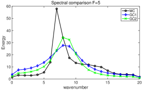
(a)

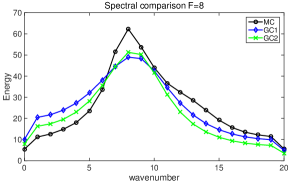
(b)

Figure 2.1: Information barriers for imperfect closure models with only consistent equilibrium single point statistics $\left(\bar{u}_{\mathrm{1pt}},r_{\mathrm{1pt}}\right)$ in the L-96 system. The steady state variances under Fourier basis from the two imperfect model results are compared with the truth from Monte-Carlo simulations in two typical dynamical regimes $F=5$ and $F=8$.

The barrier from (2.16) could become significant considering the gap between the largest and smallest variances due to common decaying energy spectra in turbulent systems. See [63] for a detailed example for the L-96 model. This information barrier can only be overcome by introducing more careful calibration about the dynamics in each eigen-direction of the system individually.

2.4.3 Dynamical calibration for imperfect model improvement

The prediction skill of imperfect models can be improved by comparing the information distance through the linear response operator with the true model. The following fact offers a convenient way to measure the lack of information in the perturbed imperfect model requiring only knowledge of linear responses for the mean and variance $\delta\bar{\mathbf{u}}\equiv\delta\mathcal{R}_{\mathbf{u}},\delta R\equiv\delta\mathcal{R}_{\left(\mathbf{u}-\bar{\mathbf{u}}\right)^{2}}$. For this result, it is important to tune the imperfect model to satisfy equilibrium model fidelity,

$$\mathcal{P}\left(p_{G}\left(\mathbf{u}\right),p_{G}^{M}\left(\mathbf{u}\right)\right)=0,$$

in the first place. Statistical equilibrium fidelity is a natural necessary condition to tune the mean and variance of the imperfect model to match those of the perfect model; it is far from a sufficient condition [54, 58, 59]. Using simplified assumptions with block-diagonal covariance matrices $R=\mathrm{diag}\left(R_{k}\right)$ and equilibrium model fidelity $\mathcal{P}\left(p_{G},p_{G}^{M}\right)=0$, the relative entropy in (2.11) between the true perturbed density $p_{\delta}$ and the perturbed model density $p_{\delta}^{M}$ with small perturbation $\delta$ can be expanded componentwisely as the following proposition:

Proposition 2.4.

Under assumptions with block-diagonal covariance matrices $R=\mathrm{diag}\left(R_{k}\right)$ and equilibrium model fidelity $\mathcal{P}\left(p_{G},p_{G}^{M}\right)=0$, the relative entropy in (2.12) between perturbed model density $p_{\delta}^{M}$ and the true perturbed density $p_{\delta}$ with small perturbation $\delta$ can be expanded componentwisely as

(2.17) $$\mathcal{P}\left(p_{\delta},p_{\delta}^{M}\right) = \mathcal{S}\left(p_{G,\delta}\right)-\mathcal{S}\left(p_{\delta}\right)$$

$$+\frac{1}{2}\sum_{k}\left(\delta\bar{u}_{k}-\delta\bar{u}_{M,k}\right)R_{k}^{-1}\left(\delta\bar{u}_{k}-\delta\bar{u}_{M,k}\right)$$

$$+\frac{1}{4}\sum_{k}R_{k}^{-2}\left(\delta R_{k}-\delta R_{M,k}\right)^{2}+O\left(\delta^{3}\right).$$

Here in the first line $\mathcal{S}\left(p_{G,\delta}\right)-\mathcal{S}\left(p_{\delta}\right)$ is the intrinsic error from Gaussian approximation of the system. $R_{k}$ is the equilibrium variance in $k$-th component, and $\delta\bar{u}_{k}$ and $\delta R_{k}$ are the linear response operators for the mean and variance in $k$-th component.

Detailed derivation about this result is shown in [59]. The inherent information error from the first row of (2.17) is due to the measurement in only first two order of moments, and is independent of the specific imperfect model structures. As a result, this component, $\mathcal{S}\left(p_{G,\delta}\right)-\mathcal{S}\left(p_{\delta}\right)$, can be viewed as a constant and does not need to be calculated in the optimization procedure. The second row of the information distance (2.17) illustrates the signal error from the estimation about the mean responses, while the third row is the dispersion error for the errors from the variance responses.

The above Proposition 2.4 about empirical information theory and linear response theory together provides a convenient and unambiguous way of improving the performance of imperfect models in terms of increasing their model sensitivity regardless of the specific form of external perturbations $\delta\mathbf{f}^{\prime}$. The formula (2.10) in Proposition 2.2 as well as (2.7) illustrates that the skill of an imperfect model in predicting forced changes to perturbations with general external forcing is directly linked to the model’s skill in estimating the linear response operators $\mathcal{R}_{A}$ for the mean and variances (that is, use the functional $A=\mathbf{u},\left(\mathbf{u}-\bar{\mathbf{u}}\right)^{2}$ in calculating the linear response operators) in a suitably weighted fashion as dictated by information theory (2.17). This offers us useful hints of training imperfect models for optimal responses for the mean and variance in a universal sense. From the linear response theory, it shows that the system’s responses to various external perturbations can be approximated by a convolution with the linear response operator $\mathcal{R}_{A}$ (which is only related to the statistics in the unperturbed equilibrium steady state). It is reasonable to claim that an imperfect model with precise prediction of this linear response operator should possess uniformly good sensitivity to different kinds of perturbations. On the other hand, the response operator can be calculated easily by the transient state distribution density function using the kicked response formula as in (2.10). Considering all these good features of the linear response operator, the information barrier due to model sensitivity to perturbations can be overcome by minimizing the information error in the imperfect model kicked response distribution relative to the true response from observation data.

To summarize, consider a class of imperfect models, $\mathcal{M}$. The optimal model $M^{*}\in\mathcal{M}$ that ensures best information consistent responses to various kinds of perturbations is characterized with the smallest additional information in the linear response operator $\mathcal{R}_{A}$ among all the imperfect models, such that

(2.18) $$\left\|\mathcal{P}\left(p_{\delta},p_{\delta}^{M^{*}}\right)\right\|_{L^{1}\left(\left[0,T\right]\right)}=\min_{M\in\mathcal{M}}\left\|\mathcal{P}\left(p_{\delta},p_{\delta}^{M}\right)\right\|_{L^{1}\left(\left[0,T\right]\right)},$$

where $p_{\delta}^{M}$ can be achieved through a kicked response procedure (2.10) in the training phase compared with the actual observed data $p_{\delta}$ in nature, and the information distance between perturbed responses $\mathcal{P}\left(p_{\delta},p_{\delta}^{M}\right)$ can be calculated with ease through the expansion formula (2.17). The information distance $\mathcal{P}\left(p_{\delta}\left(t\right),p_{\delta}^{M}\left(t\right)\right)$ is measured at each time instant, so the entire error is averaged under the $L^{1}$-norm inside a proper time window $\left[0,T\right]$ before the linear response function decays back to zero.

3 Reduced-Order Statistical Models for the Turbulent Systems

Previously in Section 2, the general idea about finding the optimal imperfect model is proposed according to the statistical theories and information distance metric. And we have shown the basic theoretical tools that can help construct the reduced-order statistical approximations and illustrate the information barriers due to these approximations. Then it is important to construct the explicit forms of the reduced-order models according to the exact dynamics for the mean and covariance in (1.4) and (1.5). Generally the statistical model for the leading two moments can be formulated in the full phase space as

(3.1a) $$\frac{d\bar{\mathbf{u}}_{M}}{dt} = \left(L+D\right)\bar{\mathbf{u}}_{M}+B\left(\bar{\mathbf{u}}_{M},\bar{\mathbf{u}}_{M}\right)+R_{M,ij}B\left(\mathbf{e}_{i},\mathbf{e}_{j}\right)+\mathbf{F},$$

(3.1b) $$\frac{dR_{M}}{dt} = L_{v}\left(\bar{\mathbf{u}}_{M}\right)R_{M}+R_{M}L_{v}^{*}\left(\bar{\mathbf{u}}_{M}\right)+Q_{F}^{M}+Q_{\sigma},$$

where $\bar{\mathbf{u}}_{M}\in\mathbb{R}^{N}$ is the model approximated mean, and $R_{M}$ is the $N\times N$ full order covariance matrix about the fluctuation state variable $\mathbf{u}^{\prime}\in\mathbb{R}^{N}$. Comparing with the original statistical dynamics (1.4) and (1.5), the most expensive but crucial part comes from the nonlinear flux term $Q_{F}$ in (1.6c) where important third-order moments are included representing the nonlinear interactions between different modes. Therefore the key issue in this section is to construct a judicious estimation about this nonlinear interaction term $Q_{F}^{M}$ in the statistical closure models. Here the basic idea is to start with the simplest possible imperfect model and compare the advantages and limitations of different levels of imperfect models due to different degrees of approximation and model calibration, and finally check how the theories from previous sections can help with improving the model prediction skill, especially the model sensitivity to various perturbations.

3.1 A hierarchy of statistical reduced-order modeling ideas based on stochastic models

We may consider the statistical closure ideas by taking another look at the dynamics for stochastic coefficients

$$\frac{dZ_{i}}{dt}=Z_{j}\left[\left(L+D\right)\mathbf{e}_{j}+B\left(\bar{\mathbf{u}},\mathbf{e}_{j}\right)+B\left(\mathbf{e}_{j},\bar{\mathbf{u}}\right)\right]\cdot\mathbf{e}_{i}+B\left(\mathbf{u}^{\prime},\mathbf{u}^{\prime}\right)\cdot\mathbf{e}_{i}+\sigma\left(t\right)\dot{\mathbf{W}}\left(t;\omega\right)\cdot\mathbf{e}_{i}.$$

Major nonlinearity comes from the term above representing interactions between different fluctuation modes $B\left(\mathbf{u}^{\prime},\mathbf{u}^{\prime}\right)\cdot\mathbf{e}_{i}$. The first idea here is to model the effect of the nonlinear energy transfers on each mode by adding additional damping $d_{M,i}$ balancing the linearly unstable character of these modes, and adding additional (white) stochastic excitation with standard deviation $\sigma_{M,i}$ which will model the energy received by the stable modes. We want to constrain ourselves to second order models concentrating on the mean and variance and maintaining the computational expense in a low level, hence the additional parts $d_{M,i},\sigma_{M,i}$ only include statistics up to second order moments. Specifically we replace this high-order nonlinear term by

$$B\left(\mathbf{u}^{\prime},\mathbf{u}^{\prime}\right)\cdot\mathbf{e}_{i}\equiv\sum_{m,n}Z_{m}Z_{n}B\left(\mathbf{e}_{m},\mathbf{e}_{n}\right)\cdot\mathbf{e}_{i}\rightarrow-d_{M,i}\left(\mathrm{tr}R\right)Z_{i}+\sigma_{M,i}\left(\mathrm{tr}R\right)\dot{W}_{i},$$

with $\mathrm{tr}R=\sum_{j}\left\langle Z_{j}Z_{j}^{*}\right\rangle$ for measuring the total energy (variance) structure in the system. Corresponding to the statistical equations, the nonlinear flux $Q_{F}$ representing the higher-order interactions is replaced by

(3.2) $$Q_{F}^{M}=Q_{F-}^{M}+Q_{F+}^{M}=-D_{M}\left(R\right)R_{M}-R_{M}D_{M}^{*}\left(R\right)+\Sigma_{M}\left(R\right).$$

In (3.2), $\left(D_{M},\Sigma_{M}\right)$ are $N\times N$ matrices that replace the original nonlinear unstable and stable effects from the original dynamics. Here $Q_{F-}^{M}=-D_{M}\left(R\right)R_{M}-R_{M}D_{M}^{*}\left(R\right)$ represents the additional damping effect to stabilize the unstable modes with positive Lyapunov coefficients, while $Q_{F+}^{M}=\Sigma_{M,k}\left(R\right)$ is the positive-definite additional noise to compensate for the overdamped modes. Now the problem is converted to finding expressions for $D_{M}$ and $\Sigma_{M}$. In the following by gradually adding more detailed characterization about the statistical dynamical model we display the general procedure of constructing a hierarchy of the closure methods step by step. Below is a review about several model closure ideas [54, 88, 63, 78] with increasing complexity:

1. Quasilinear Gaussian closure model: The simplest approximation for the closure methods at the first stage should be simply neglecting the nonlinear part entirely [23, 25, 90]. That is, set

   (3.3) $$D_{M}\left(R\right)\equiv 0,\quad\Sigma_{M}\left(R\right)\equiv 0,\qquad Q_{F}^{\mathrm{QG}}\equiv 0.$$

   Thus the nonlinear energy transfer mechanism will be entirely neglected in this Gaussian closure model. This is the similar idea in the eddy-damped Markovian model where the moment hierarchy is closed at the level of second moments with Gaussian assumption and a much larger eddy-damped parameter is introduced to replace the molecular viscosity (see Chapter 5 of [84] and [44] for details). Obviously this crude Gaussian approximation will not work well in general due to the cutoff of the energy flow when strong nonlinear interactions between modes occur. Actually, the deficiency of this crude approximation have been shown under the L-96 framework, and in final equilibrium state there exists only one active mode with critical wavenumber [89, 63]. Such closures are only useful in the weakly nonlinear case where the quasi-linear effects are dominant.

2. Models with consistent equilibrium statistics: Next the strategy is to construct the simplest closure model with consistent equilibrium statistics. So the direct way is to choose constant damping and noise term at most scaled with the total variance. We propose two possible choices as in [63] for the damping and noise in (3.2) below.
   Gaussian closure 1 (GC1): let

   (3.4) $$D_{M}\left(R\right)=\epsilon_{M}I_{N}\equiv\mathrm{const.},\quad\Sigma_{M}\left(R\right)=\sigma_{M}^{2}I_{N}\equiv\mathrm{const.},\qquad Q_{F}^{\mathrm{GC1}}=-\left(\epsilon_{M}R+R\epsilon_{M}\right)+\sigma_{M}^{2}I_{N};$$

   
   

   Gaussian closure 2 (GC2): let

   (3.5) $$D_{M}\left(R\right)=\epsilon_{M}\left(\frac{\mathrm{tr}R}{\mathrm{tr}R_{\mathrm{eq}}}\right)^{1/2}I_{N},\quad\Sigma_{M}\left(R\right)=\sigma_{M}^{2}\left(\frac{\mathrm{tr}R}{\mathrm{tr}R_{\mathrm{eq}}}\right)^{3/2}I_{N},\quad Q_{F}^{\mathrm{GC2}}=-\left(\frac{\mathrm{tr}R}{\mathrm{tr}R_{\mathrm{eq}}}\right)^{1/2}\left(\epsilon_{M}R+R\epsilon_{M}\right)+\sigma_{M}^{2}\left(\frac{\mathrm{tr}R}{\mathrm{tr}R_{\mathrm{eq}}}\right)^{3/2}I_{N}.$$

   Above only two scalar model parameters $\left(\epsilon_{M},\sigma_{M}\right)$ are introduced, and $I_{N}$ represents the $N\times N$ identity matrix. GC1 is the familiar strategy of adding constant damping and white noise forcing to represent nonlinear interaction; GC2 scales with the total variance $\mathrm{tr}R$ (or total statistical energy) so that the model sensitivity can be further improved as the system is perturbed. From both GC1 and GC2, we introduce uniform additional damping rate for each spectral mode controlled by a single scalar parameter $\epsilon_{M}$; while the additional noise with variance $\sigma_{M}^{2}$ is added to make sure climate fidelity in equilibrium (we leave the detailed discussion for climate fidelity in Section 3.2.1).
   The statistical model closure $Q_{F}^{M}$ is used to approximate the third-order moments in the true dynamics, thus the exponents of the total energy $\mathrm{tr}R$ in GC2 should be consistent in scaling dimension. In the positive-definite part $Q_{F+}^{M}$, it calibrates the rate of energy injected into the spectral mode due to nonlinear effect in the order $\left|u^{\prime}\right|^{3}$. The factor scales with the total energy with exponent $3/2$ so that the corrections keep consistent with the third-order moment approximations; In the negative damping rate $Q_{F-}^{M}$, the scaling function is used to characterize the amount of energy that flows out the spectral mode due to nonlinear interactions. Scaling factor with a square-root of the total energy with exponent $1/2$ is applied for this damping rate multiplying the variance in order $\left|u^{\prime}\right|^{2}$ to make it consistent in scaling dimension with third moments.

3. Modified quasi-Gaussian closure with equilibrium statistics: In this modified quasi-Gaussian closure model originally proposed in [89, 88], we exploit more about the true nonlinear energy transfer mechanism from the equilibrium statistical information. Thus the additional damping and noise proposed like before are calibrated through the equilibrium nonlinear flux by letting

   (3.6) $$D_{M}\left(R\right)=-N_{M,\mathrm{eq}},\quad\Sigma_{M}\left(R\right)=Q_{F,\mathrm{eq}}^{+},\qquad Q_{F}^{\mathrm{MQG}}=-\left(N_{M}R+RN_{M}^{*}\right)+Q_{F}^{+};.$$

   $N_{M,\mathrm{eq}}$ is the effective damping from equilibrium, and $Q_{F,\mathrm{eq}}^{+}$ is the effective noise from the positive-definite component. Unperturbed equilibrium statistics in the nonlinear flux $Q_{F,\mathrm{eq}}$ are used to calibrate the higher-order moments as additional energy sink and source. The true equilibrium higher-order flux can be calculated without error from first and second order moments in $\left(\bar{\mathbf{u}}_{\mathrm{eq}},R_{\mathrm{eq}}\right)$ from the unperturbed true dynamics (1.5) in steady state following the steady state statistical solution relation (2.3) as discussed in Section 2.2

   (3.7) $$Q_{F,\mathrm{eq}}=Q_{F,\mathrm{eq}}^{-}+Q_{F,\mathrm{eq}}^{+}=-L_{v}\left(\bar{\mathbf{u}}_{\mathrm{eq}}\right)R_{\mathrm{eq}}-R_{\mathrm{eq}}L_{v}^{*}\left(\bar{\mathbf{u}}_{\mathrm{eq}}\right)-Q_{\sigma},\quad N_{M,\mathrm{eq}}=\frac{1}{2}Q_{F,\mathrm{eq}}^{-}R_{\mathrm{eq}}^{-1}.$$

   $Q_{F,\mathrm{eq}}^{-},Q_{F,\mathrm{eq}}^{+}$ are the negative and positive definite components in the unperturbed equilibrium nonlinear flux $Q_{F,\mathrm{eq}}$. Since exact model statistics are used in the imperfect model approximations, the true mechanism in the nonlinear energy transfer can be modeled under this first correction form. This is the similar idea used for measuring higher-order interactions in [88], where more sophisticated and expensive calibrations are required to make that model work there.

3.2 A reduced-order statistical energy model with optimal consistency and sensitivity

The above closure model ideas, especially (3.4), (3.5), and (3.6), have advantages of their own. Models in (3.4) and (3.5) are simple and efficient to construct with consistent equilibrium consistency, while (3.6) involves the true information about the higher-order statistics in equilibrium so that the energy mechanism can be characterized well. The validity of these approaches has been tested and compared from several papers [89, 88, 63] using the simplified triad model and L-96 model. Still when it comes to the more complicated and realistic flow systems like the quasi-geostrophic equations, more detailed calibration for model consistency and sensitivity is required to achieve the optimal performance. A preferred approach for the nonlinear flux $Q_{F}^{M}$ combining both the detailed model energy mechanism and control over model sensitivity is proposed in the form

(3.8) $$Q_{F}^{M}=Q_{F}^{M,-}+Q_{F}^{M,+}=f_{1}\left(R\right)\left[-\left(N_{M,\mathrm{eq}}+d_{M}I_{N}\right)R_{M}\right]+f_{2}\left(R\right)\left[Q_{F,\mathrm{eq}}^{+}+\Sigma_{M}\right].$$

The closure form (3.8) consists of three indispensable components:

i)

Higher-order corrections from equilibrium statistics: In the first part of the correction using the damping and noise operator as $\left(N_{M,\mathrm{eq}},Q_{F,\mathrm{eq}}^{+}\right)$, unperturbed equilibrium statistics in the nonlinear flux $Q_{F,\mathrm{eq}}$ are used to calibrate the higher-order moments as additional energy sink and source following the procedure in (3.6). Therefore the equilibrium statistics can be guaranteed to be consistent with the truth, and the true energy mechanism can be restored;

ii)

Additional damping and noise to model changes in nonlinear flux: The above corrections in step i) by using equilibrium information for nonlinear flux is found to be insufficient for accurate prediction in the reduced-order methods since the scheme is only marginally stable and the energy transferring mechanism may change with large deviation from the equilibrium case when external perturbations are applied. Thus we also introduce the additional damping and noise $\left(d_{M},\Sigma_{M}\right)$ as from (3.4). $d_{M}$ is just a constant scalar parameter to add uniform dissipation on each mode, and $\Sigma_{M}$ is the further correction as an additional energy source to maintain climate fidelity;

iii)

Statistical energy scaling to improve model sensitivity: Still note that these additional parameters are added regardless of the true nonlinear perturbed energy mechanism where only unperturbed equilibrium statistics are used. To capture the responses to a specific perturbation forcing, it is better to make the imperfect model parameters change adaptively according to the total energy structure. Considering this, the additional damping and noise corrections are scaled with factors $f_{1}\left(R\right),f_{2}\left(R\right)$ related with the total statistical variance $\mathrm{tr}R$ as

(3.9) $$f_{1}\left(R\right)=\left(\frac{\mathrm{tr}R}{\mathrm{tr}R_{\mathrm{eq}}}\right)^{1/2},\quad f_{2}\left(R\right)=\left(\frac{\mathrm{tr}R}{\mathrm{tr}R_{\mathrm{eq}}}\right)^{3/2}.$$

Note that in the full model formulation (3.1a) and (3.1b) with the entire covariance matrix $R$ resolved, the total variance structure $\mathrm{tr}R$ is easy to achieve. However in the low-order models with only the variances in the principal modes resolved explicitly as will be discussed in the following subsection, $\mathrm{tr}R$ is generally not available directly. This is where the statistical energy dynamics (2.2) can play an important role and help the development of reduced order models. Besides, a further skew-symmetric correction for dispersion effects in addition to the scalar model damping $d_{M}$ in the reduced-order models might be useful in some situations as the following remark.

Remark 3.1.

In the additional damping correction in (3.8), only a scalar damping parameter $d_{M}$ is considered. A little more detailed calibration about the nonlinear exchange of energy is to also introduce an imaginary skew-symmetric operator $i\Omega_{M}$ applied on the covariance $R_{M}$, that is,

$$Q_{F}^{M,-}=\left(-d_{M}I_{N}+i\Omega_{M}\right)R_{M}$$

This term will not alter the entire energy structure of the system due to skew symmetry but can offer correction for the dispersion relation in this imperfect model. However, we may have the additional difficulty in fitting the $N$ by $N$ parameter matrix in the general case. In practical applications, instead we can exploit the physical structure of the specific model and introduce only one additional dispersion parameter $i\omega_{M}$; see [78] and [79] for two examples of adding the dispersion correction to effectively improve model prediction skill under the barotropic and baroclinic models.

Next we discuss the detailed calibrations about the nonlinear flux approximations. Two steps of model calibration should be considered as from the general framework described in Section 1.2: i) the equilibrium consistency that the reduced model must converge to the true equilibrium statistical state as no perturbations are added; ii) model sensitivity by blending statistical response and information theory so that the imperfect model can capture the responses to various kinds of perturbations as the system is perturbed. The construction in (3.6) guarantees equilibrium consistency using the true equilibrium model nonlinear flux structure. On the other hand, to improve model sensitivity, the linear response operators with information distance metric are used to find optimal parameters from the correction part in (3.4) or (3.5).

3.2.1 Equilibrium statistical fidelity through the additional damping and noise

In designing the reduced-order models, equilibrium fidelity for consistent statistics should be guaranteed in the first place in the unperturbed climate. That is, the same final unperturbed statistical equilibrium $R_{\mathrm{eq}}$ should be recovered from the closure models $R_{M}$ in each component. Comparing the true statistical equation (1.5) with the reduced-order model (3.1b), time derivatives about the statistics on the left hand sides vanish in statistical steady state, thus climate consistency can be achieved if we have exact recovery of the estimation in the nonlinear flux term. Specifically, it requires that the model nonlinear flux correction term (3.8) converges to the truth, $Q_{M}\rightarrow Q_{F,\mathrm{eq}}$, when no external perturbation is added. Under this condition in steady state the closure model covariance equation (3.1b) goes to the true unperturbed statistics, the equilibrium statistical relation (2.3) implies the relation

$$0=L_{v}\left(\bar{\mathbf{u}}_{\mathrm{eq}}\right)R_{M,\mathrm{eq}}+R_{M,\mathrm{eq}}L_{v}^{*}\left(\bar{\mathbf{u}}_{\mathrm{eq}}\right)+Q_{F,\mathrm{eq}}^{M}+Q_{\sigma}\;\rightarrow\;R_{M,\mathrm{eq}}=R_{\mathrm{eq}}.$$

In construction the first component $\left(N_{M,\mathrm{eq}},Q_{F,\mathrm{eq}}^{+}\right)$ comes from the true equilibrium statistics, and in equilibrium state it will guarantee the consistency with the truth that

$$-\left(N_{M,\mathrm{eq}}R_{\mathrm{eq}}+R_{\mathrm{eq}}N_{M,\mathrm{eq}}^{*}\right)+Q_{F,\mathrm{eq}}^{+}=Q_{F,\mathrm{eq}}.$$

This part will be automatically equal to the true nonlinear flux in equilibrium. On the other hand climate consistency requires that the second component correction due to the parameters $\left(d_{M}I_{N},\Sigma_{M}\right)$ adds no additional energy source or sink in the unperturbed system, and no further correction in the scaling functionals. That is, we need $\Sigma_{M}$ to satisfy

(3.10) $$\Sigma_{M}=\frac{1}{2}d_{M}R_{\mathrm{eq}},\quad f_{1}\left(\mathrm{tr}R_{\mathrm{eq}}\right)=1,\;f_{2}\left(\mathrm{tr}R_{\mathrm{eq}}\right)=1.$$

Note again $f_{1}$ and $f_{2}$ in (3.10) calibrate the model sensitivity to perturbations according to the total energy structure $\mathrm{tr}R$. Thus it is natural to assume no additional correction in the unperturbed case.

By choosing parameters according to (3.10), the climate consistency for the imperfect reduced-order models in (3.1b) in the unperturbed equilibrium is guaranteed. In addition, we still leave one controlling parameter $d_{M}$ for the freedom to tune the imperfect model performance, considering that climate consistency is only the necessary but not sufficient condition for good model prediction [59].

3.2.2 Model calibration blending statistical response and information theory

The above methods (3.4), (3.5), (3.6), as well as (3.8) construct statistical approximation models with consistent equilibrium statistics. Still equilibrium fidelity of imperfect models is a necessary but not sufficient condition for model prediction skill with many examples [54, 59, 63]. In order to get precise forecasts for various forced responses, it is also crucial to seek models that can correctly reflect the system’s ‘memory’ to its previous states. From Section 2.2, it shows that the linear response operator $\mathcal{R}_{A}$ represents the lagged-covariance of certain functions (and thus can describe the ‘memory’ of the system to previous states). We try to find a unified way to achieve the optimal model parameters $d_{M}$ such that the imperfect models can maintain high performance for various kinds of external perturbations. Adopting the general strategy suggested in Section 2.3, we can improve model sensitivity through tuning imperfect models in a training phase before the prediction step. Thus the optimal model parameter can be selected through minimizing the information distance in the linear response operators in (2.18) between the imperfect closure model and the truth.

Information-theoretical framework to measure the linear responses in the training phase

In this training phase, we try to find the optimal model parameters $d_{M}$ by comparing the linear response operators from the true system and imperfect approximation model. The true model linear response operator and the reduced-order model response operator can be calculated from (2.8), following the procedure from the kicked response strategy with detailed procedure shown in Appendix A. The distance between these two operators can be calculated through the information metric (2.17) which offers an unbiased and invariant measure for model distributions

$$\mathcal{P}\left(p_{\delta},p_{\delta}^{M}\right) = \frac{1}{2}\sum_{k}\left(\delta\bar{u}_{k}-\delta\bar{u}_{M,k}\right)R_{k}^{-1}\left(\delta\bar{u}_{k}-\delta\bar{u}_{M,k}\right)$$

$$+\frac{1}{4}\sum_{k}R_{k}^{-2}\left(\delta R_{k}-\delta R_{M,k}\right)^{2}+O\left(\delta^{3}\right).$$

The first row above is the signal error due to the estimation about the mean; and the second row is the dispersion error for calibrating the linear responses in the first two order of moments, $\delta R_{\mathbf{k}}$. The intrinsic error due to second-order closure $\mathcal{S}\left(p_{G,\delta}\right)-\mathcal{S}\left(p_{\delta}\right)$ is independent of the specific forms of the reduced-order models and is not included in this metric. The optimization principle in (2.18) is then performed over the parameter $d_{M}$.

3.2.3 Comparisons with stochastic modeling about the mean and fluctuations and realizability

To achieve a better understanding about the statistical models, it is useful to compare the reduced-order statistical energy model (3.1a) and (3.1b) with its stochastic correspondences. In the stochastic formulation, we consider the separation with a deterministic mean state and the stochastic fluctuations

$$\mathbf{u}_{M}=\bar{\mathbf{u}}_{M}\left(t\right)+\sum_{j}Z_{j}\left(t\right)\mathbf{e}_{j},$$

where $\bar{\mathbf{u}}_{M}=\left\langle\mathbf{u}_{M}\right\rangle$ is the statistical mean state following the same dynamical mean equation as before together with the stochastic dynamics for the fluctuation modes

(3.11a) $$\frac{d\bar{\mathbf{u}}_{M}}{dt} = \left(L+D\right)\bar{\mathbf{u}}_{M}+B\left(\bar{\mathbf{u}}_{M},\bar{\mathbf{u}}_{M}\right)+\left\langle Z_{i}Z_{j}^{*}\right\rangle B\left(\mathbf{e}_{i},\mathbf{e}_{j}\right)+\mathbf{F},$$

(3.11b) $$\frac{dZ_{i}}{dt} = Z_{j}\left[\left(L+D\right)\mathbf{e}_{j}+B\left(\bar{\mathbf{u}}_{M},\mathbf{e}_{j}\right)+B\left(\mathbf{e}_{j},\bar{\mathbf{u}}_{M}\right)\right]\cdot\mathbf{e}_{i}\>-d_{M,i}\left(\left\langle\mathbf{ZZ^{*}}\right\rangle\right)Z_{i}+\Sigma_{M,ij}\left(\left\langle\mathbf{ZZ^{*}}\right\rangle\right)\dot{W}_{ij}.$$

Above the effective damping and noise $\left(d_{M}I_{N},\Sigma_{M}\right)$ are added in the same way as constructed in (3.8). The mean dynamics (3.11a) get the small scale feedbacks from the nonlinear statistical interaction $\left\langle Z_{i}Z_{j}^{*}\right\rangle B\left(\mathbf{e}_{i},\mathbf{e}_{j}\right)$, while the fluctuation stochastic dynamics are linked with the mean state through the quasilinear interactions. By direct comparison with the statistical equations (3.1a) and (3.1b), we see that the mean equation is identical while the equation for the stochastic fluctuations differs in the nonlinear term. The constructed set of closed stochastic equations is a representative of a new class of stochastic systems where the evolution of each stochastic realization depends on the global statistics, i.e. on the collective or statistical behavior of all the realizations due to $\left\langle\mathbf{ZZ^{*}}\right\rangle$. In particular, the associated formal Fokker-Planck equation becomes nonlinear and nonlocal. This guarantees realizability of the reduced-order models. These novel stochastic equations deserve further mathematical study as a complex version of McKean-Vlasov systems [69].

3.3 Reduced-order statistical model for principal modes

Here for genuinely high-dimensional systems, the computational cost for the full covariance matrix $R_{M}$ is still unaffordable even with the first two moment closure [6, 56]; for example, climate systems usually have the dimensionality at least of order $10^{3}$ . On the other hand, in many situations, we are mostly interested in the variability in the statistics of the first most energetic principal directions. Therefore one alternative practical strategy is to develop reduced-order methods that only calculate variances in a low-dimensional subspace spanned by primary EOFs $\left\{\mathbf{v}_{1},\cdots,\mathbf{v}_{s}\right\}$ with $s\ll N$ ($N$ the dimensionality of the full system). The corresponding reduced-order representation of the state variables under these resolved basis becomes $\mathbf{u}=\bar{\mathbf{u}}+\sum_{k=1}^{s}Y_{k}\mathbf{v}_{k}$. To see the possibility of achieving this, first note that the dynamical equations for variances (3.1b) in each mode $r_{k}=\left\langle Y_{k}Y_{k}^{*}\right\rangle$ are rather independent with each other according to the previous closure strategies with higher-order interactions replaced by additional damping and noise terms. Thus it is realizable to restrict the variance equations inside the chosen subspace. Actually following the same strategy by replacing the high-order interaction terms by proper damping and noise, the equivalent counterpart of the closure models can be formulated as a low-order stochastic system

(3.12a) $$\frac{d\bar{\mathbf{u}}_{M}}{dt} = \left(L+D\right)\bar{\mathbf{u}}_{M}+B\left(\bar{\mathbf{u}}_{M},\bar{\mathbf{u}}_{M}\right)+\sum_{i,j\leq s}C_{M,ij}B\left(\mathbf{v}_{i},\mathbf{v}_{j}\right)+\mathbf{F}+\mathbf{G},$$

(3.12b) $$\frac{dC_{M}}{dt} = L_{v}^{\mathrm{red}}C_{M}+C_{M}L_{v}^{\mathrm{red}*}+Q_{F,M}^{\mathrm{red}}+Q_{\sigma}^{\mathrm{red}},\quad C_{M}\in\mathbb{C}^{s\times s}.$$

The mean dynamics (3.12a) is the same as the previous closure model (3.1a) with an additional correction term $\mathbf{G}$ to compensate the unresolved modes. $C_{M}$ is the reduced-order $s\times s$ covariance matrix where only the leading primary modes are resolved, that is,

$$C_{M}=P^{*}R_{M}P,$$

where $P=\left[\mathbf{v}_{1},\mathbf{v}_{2},\cdots,\mathbf{v}_{s}\right]\in\mathbb{C}^{N\times s}$ projects the modes to the subspace.

Through proper choice of the parameters according to GC1 (3.4), GC2 (3.5), MQG (3.6), or the blended method (3.8) as before but concentrating on the resolved subspace, these reduced system should converge to the same first two order statistics with the moment closure model. Still several new problems need to be taken care of for the above model reduction process: i) How to ensure correct modeling about the true statistics in the mean dynamics (3.12a) due to the many unresolved directions in the covariance $C_{M}$; ii) How to include the nonlocal scale factor (which always includes the total energy $\mathrm{tr}R=\sum_{k=1}^{N}r_{k}$) in (3.9) in the nonlinear flux approximation $Q_{F,M}^{\mathrm{red}}$ if only subspace variances are resolved. Here in the general strategy to do this, we follow the ideas in [63, 78, 79].

3.3.1 Correction for the mean dynamics

Still the simplest way of estimating the unresolved parts in the mean dynamics is through the statistical equilibrium information $\mathbf{G}_{\mathrm{eq}}$. The value of the additional forcing $\mathbf{G_{\mathrm{eq}}}$ is determined using statistical steady state information for the covariance $C_{\mathrm{eq}}$ and the mean $\bar{\mathbf{u}}_{\mathrm{eq}}$. In particular we have the equilibrium equation through the steady state mean dynamics where $\frac{d}{dt}\bar{\mathbf{u}}_{\mathrm{eq}}\equiv 0$

(3.13) $$\mathbf{G_{\mathrm{eq}}}=-\left(L+D\right)\bar{\mathbf{u}}_{\mathrm{eq}}+B\left(\bar{\mathbf{u}}_{\mathrm{eq}},\bar{\mathbf{u}}_{\mathrm{eq}}\right)-\sum_{i,j\leq s}C_{\mathrm{eq},ij}B\left(\mathbf{v}_{i},\mathbf{v}_{j}\right)-\mathbf{F}_{\mathrm{eq}}.$$

Similar as in the estimation about the nonlinear flux, the mean dynamics correction term can also be scaled with the total variance in the system, so that,

(3.14) $$\mathbf{G}=\frac{\mathrm{tr}R}{\mathrm{tr}R_{\mathrm{eq}}}\mathbf{G}_{\mathrm{eq}}.$$

In this way, the mean dynamics (3.12a) become consistent in the statistical equilibrium state, and the corrections $\mathbf{G}$ can change sensitively according to the total energy structure through $\mathrm{tr}R$.

Remark 3.2.

One further optional correction for the unresolved modes in the reduced-order mean equations is to make further use of the linear response theory predictions. To estimate the values for unresolved modes, we can improve it from the equilibrium statistics by introducing finer approximation making use of the linear response operator (2.7)

(3.15) $$r_{k,\mathrm{un}}\sim r_{k,\mathrm{eq}}+\delta r_{k}^{\prime}=r_{k,\mathrm{eq}}+\int_{0}^{t}\mathcal{R}_{r_{k}}\left(t-s\right)\delta F^{\prime}\left(s\right)ds,\quad k>s.$$

Therefore these first-order predictions for the unresolved variances $r_{k,\mathrm{un}}$ can also be used in (3.12a) for estimating the unresolved modes. This idea is applied to the L-96 system with improvements shown in [63].

3.3.2 Correction through total statistical energy

In the reduced-order covariance dynamics (3.12b) using the closure form (3.8), two additional scaling factors, $f_{1},f_{2}$, are introduced to further quantify the nonlinear energy flux in and out the spectral modes due to the nonlinear interactions. We propose the dynamical corrections with the total statistical energy $\mathrm{tr}R$ as in the forms (3.9). This total energy correction introduces global information into each spectral mode so the nonlinear energy transfer can be better characterized in the imperfect model, while solving only one additional scalar equation is the only additional cost in computation. The scaling factor from $\mathrm{tr}R$ introduces nonlinear global effect into the additional damping and noise corrections in each mode. This can be solved efficiently by introducing one additional scalar equation as described in (2.2)

$$\frac{dE}{dt}=\bar{\mathbf{u}}\cdot D\bar{\mathbf{u}}+\bar{\mathbf{u}}\cdot\mathbf{F}+\mathrm{tr}\left(DR\right)+\frac{1}{2}\mathrm{tr}Q_{\sigma}.$$

Then $\mathrm{tr}R$ can be achieved by solving $E=\frac{1}{2}\bar{\mathbf{u}}^{2}+\frac{1}{2}\mathrm{tr}R$.

Especially in uniform damping case, $D=-dI$, the above statistical energy equation can be simplified as

(3.16) $$\frac{dE}{dt}=-dE+\bar{\mathbf{u}}\cdot\mathbf{F}+\frac{1}{2}\mathrm{tr}Q_{\sigma}.$$

Note that on the right hand side of (3.16), only mean state information (which can be fully resolved in the reduced mean dynamics in (3.12a)) needs to be calculated to get the total statistical energy $E$. In this way, the total second order moments $\mathrm{tr}R$ can be entirely determined only through the first order mean $\bar{\mathbf{u}}$ and the scalar statistical energy equation (3.16).

The final issue in the reduced-order model construction is about the tuning process in the training phase. Still the same kicked-response strategy (2.10) can be applied to the reduced-order formulation (3.12). Importantly, the relative entropy expansion for the responses in (2.17) is decomposed into each component. Thus it can be directly applied to the reduced-order case by calculating only the signal and dispersion error in the resolved subspace. Therefore through the same procedure as the previous case, we can find the optimal model parameter in the training phase for the reduced-order model, and then apply the optimal model for prediction with various forcing perturbations.

3.4 Summary of the Reduced-Order Statistical Energy Closure algorithm

We summarize the low-dimensional reduced-order statistical closure algorithm with calibrations from total statistical energy and linear response theory. The general reduced-order model algorithm is split into the separated steps of a training phase and a prediction phase after a proper imperfect model selection step according to the problem. The training phase is used to improve model sensitivity by tuning the imperfect model parameter using only unperturbed equilibrium statistics for the linear response operator. Then the optimal parameter can be applied for predicting model responses to different kinds of external perturbations.

Algorithm 1 Reduced-order statistical closure model for general turbulent systems

• Model selection stage:

  • Decide the low-dimensional subspace spanned by orthonormal basis $\left\{\mathbf{v}_{k}\right\}_{k=-s}^{s}$ covering the directions with largest variances (energy) among the spectrum.

  • Set up statistical dynamical equations (3.12) by Galerkin projecting the original equations to the resolved subspace for modes with wavenumbers $1\leq\left|k\right|\leq s$, as well as the statistical energy equation (3.16) to get the total statistical energy $E_{M}$ in the system.

• Model calibration stage:

  • Construct low-order approximation of the nonlinear flux $Q_{F}^{M}$ in the statistical equations using the statistical energy closure proposed in (3.8) consistent with the equilibrium first two moments;

  • Compute the true linear response operator from the unperturbed equilibrium statistics, and calculate the imperfect model predicted linear response operator from the kicked response strategy;

  • Determine the imperfect model parameter value through minimizing the information distance in (2.17) and (2.18) between linear response operators from true equilibrium statistics and imperfect model approximation.

• Model prediction stage:

  • Use the optimally tuned parameter achieved from the previous step in the reduced-order model to get statistical responses of the state variables of interest in principal directions with all kinds of specific external perturbations.

Note that in the calibration step in the algorithm, only the unperturbed statistics in equilibrium are required. Thus this offers the optimal model parameters that are ideally valid for all kinds of specific forcing perturbation forms. With the help of the linear response operator we are able to find a unified way to tune the imperfect model parameters and avoid the exhausting and impractical process to tune the models each time with different kinds of perturbations.

4 Reduced-Order Statistical Models Applied to a Suite of Stochastic Triad Models

In this section, we illustrate the performance of the reduced-order formulations by considering a simple but nevertheless instructive model, namely the triad system with stochastic forcing [30, 50, 54, 89]. The triad systems where three modes interact through quadratic energy-conserving nonlinear interactions form the building block for more general complex turbulent flow, thus provide a nice simple test case for the mode elimination strategy in the first stage. The nonlinear interaction in triad systems is generic of nonlinear coupling between any three modes in larger systems with quadratic nonlinearity. For a three-dimensional system about state variables $\mathbf{u}=\left(u_{1},u_{2},u_{3}\right)^{T}\in\mathbb{R}^{3}$ with a quadratic part that is energy preserving, the triad system possesses the general form

(4.1a) $$\frac{du_{1}}{dt} = L_{2}u_{3}-L_{3}u_{2}-d_{1}u_{1}+B_{1}u_{2}u_{3}+F_{1}+\sigma_{1}\dot{W}_{1},$$

(4.1b) $$\frac{du_{2}}{dt} = L_{3}u_{1}-L_{1}u_{3}-d_{2}u_{2}+B_{2}u_{3}u_{1}+F_{2}+\sigma_{2}\dot{W}_{2},$$

(4.1c) $$\frac{du_{3}}{dt} = L_{1}u_{2}-L_{2}u_{1}-d_{3}u_{3}+B_{3}u_{1}u_{2}+F_{3}+\sigma_{3}\dot{W_{3}}.$$

The triad system (4.1) is easy to summarize in the original abstract formulation (1.1), where

$$L=\begin{bmatrix}0&-L_{3}&L_{2}\\ L_{3}&0&-L_{1}\\ -L_{2}&L_{1}&0\end{bmatrix},\quad D=\begin{bmatrix}-d_{1}\\ &-d_{2}\\ &&-d_{3}\end{bmatrix},$$

are the skew-symmetric and dissipation operator in (1.2a) representing respectively the Coriolis forcing and dissipation; and $B\left(\mathbf{u},\mathbf{u}\right)$ satisfies

$$B\left(\mathbf{u},\mathbf{u}\right)=\left(B_{1}u_{2}u_{3},B_{2}u_{3}u_{1},B_{3}u_{1}u_{2}\right)^{T},\quad B_{1}+B_{2}+B_{3}=0,$$

which forms the nonlinear triad coupling that satisfies the energy conservation in (1.2b). The triad system can form the building block of complex turbulent dynamical systems since it can be viewed as a three-dimensional Galerkin truncation of many general dynamics. One celebrated example is the famous Lorenz model [45] that can be viewed as a special case of this procedure. An interpretation of these low-order models with atmospheric problems and geoscience is illustrated in [30]. Though simple in appearance of this triad system, complex and interesting statistical features can be generated through changing the model parameters.

4.1 Statistical properties for the triad system

First we can check the general statistical properties described in Section 1.2 with the triad system. Typically we would like to investigate the evolution of a smooth probability density function $p\left(\mathbf{u},t\right)$ due to the internal and external stochasticity. Associated with the triad equations (4.1), the statistical solution satisfies the Fokker-Planck equation

(4.2) $$\frac{\partial p}{\partial t} =-\left(B\left(\mathbf{u},\mathbf{u}\right)+\left(L+D\right)\mathbf{u}+\mathbf{F}\right)\cdot\nabla_{\mathbf{u}}p+\sum_{i=1}^{3}\left(d_{i}p+\frac{1}{2}\sigma_{i}^{2}\partial_{u_{i}}^{2}p\right),$$

$$p\left(\mathbf{u},t\right)\mid_{t=0} =p_{0}\left(\mathbf{u}\right).$$

Above we assume the forcing terms are only dependent on time, $\mathbf{F}\equiv\mathbf{F}\left(t\right),\sigma_{i}\equiv\sigma_{i}\left(t\right)$. While the original triad system (4.1) is nonlinear, the statistical dynamics in (4.2) are linear equation for smooth functions $p$. The Fokker-Planck equation will reduce to the Liouville equation in the case of zero stochastic noise $\sigma\equiv 0$. However the explicit solution of the Fokker-Planck equation (4.2) is still difficult to get directly even with the triad model.

4.1.1 Equilibrium invariant measure with equipartition of energy

In general the explicit solutions for the Fokker-Planck equation above (4.2) is difficult to achieve due to the nonlinear interactions in the triad system. Still under special arrangement about the damping and noise coefficients, one special solution of a Gaussian invariant measure, $p_{\mathrm{eq}}$, can be reached in the equilibrium. In the absence of the deterministic forcing, $\mathbf{F=0}$, assume the damping operator $d_{i}$ and random noise forcing $\sigma_{i}$ satisfy the following relation in each component

(4.3) $$\sigma_{\mathrm{eq}}^{2}=\frac{\sigma_{1}^{2}}{2d_{1}}=\frac{\sigma_{2}^{2}}{2d_{2}}=\frac{\sigma_{3}^{2}}{2d_{3}}.$$

Therefore, a Gaussian invariant measure as defined in (1.7) can be found with equipartition of energy in each component, that is,

(4.4) $$p_{\mathrm{eq}}=C^{-1}\exp\left(-\frac{1}{2}\sigma_{\mathrm{eq}}^{-1}\mathbf{u}\cdot\mathbf{u}\right).$$

Above $\sigma_{\mathrm{eq}}^{2}$ is the equilibrium variance in the Gaussian invariant distribution $p_{\mathrm{eq}}$ that controls the variability in each mode. To see this, we can substitute the invariant measure (4.4) back into the Fokker-Planck equation (4.2). It is a special case from the Theorem in [54], and detailed energy mechanism and stability for the triad system can be found in [50].

In the general case with deterministic external forcing and inhomogeneous structure, energy is injected into the modes and transferred to each other due to the nonlinear quadratic interaction through more complicated mechanism, thus strong nonlinear non-Gaussian statistics with energy cascade and internal instabilities can be generated.

4.1.2 A link with quasi-geostrophic turbulence

The triad model (4.1) is the building block of complex turbulent dynamical systems since a three-dimensional Galerkin truncation of many complex turbulent dynamics possesses the energy-conserving nonlinearity as in (1.1). The random forcing together with the damping term represents the inhomogeneous effect of the interaction with other modes in a turbulent dynamical system that are not resolved in the three dimensional subspace. Stochastic triad models are qualitative models for a wide variety of turbulent phenomena regarding energy exchange and cascades and supply important intuition for many effects. They also provide elementary test models with subtle features for prediction, UQ, and state estimation [50, 64, 87].

As a simple illustration about the link to more complex turbulent systems, we can consider the quasi-geostrophic (QG) potential vorticity equation with no external forcing and dissipation

$$\frac{\partial q}{\partial t}+\nabla^{\bot}\psi\cdot\nabla q=0,\quad q=\nabla^{2}\psi.$$

We have the barotropic triads of three barotropic components, $\psi_{\mathbf{k}},\psi_{\mathbf{m}},\psi_{\mathbf{n}}$, obeying the selecting rule $\mathbf{k+m+n=0}$. Consider an initial condition in which only these three components of a particular triad are excited, then these three modes will only interact with each other while no other modes will get excited due to the particular triad relations as the system evolves in time. By projecting the above equation to the active triad modes, we get the dynamical equations for the selected modes

(4.5) $$\frac{d\psi_{\mathbf{k}}}{dt}+A_{\mathbf{kmn}}\psi_{\mathbf{m}}\psi_{\mathbf{n}}=0,\quad\mathbf{k+m+n=0},$$

where $A_{\mathbf{kmn}}=\frac{\left|\mathbf{n}\right|^{2}}{\left|\mathbf{k}\right|^{2}}\mathbf{m^{\bot}\cdot n}$ is the triad interaction coefficient with the detailed symmetry $A_{kmn}+A_{mnk}+A_{nkm}=0$, showing the conservation of kinetic energy,

$$\frac{d}{dt}\left(\left|\mathbf{k}\right|^{2}\left|\psi_{\mathbf{k}}\right|^{2}+\left|\mathbf{m}\right|^{2}\left|\psi_{\mathbf{m}}\right|^{2}+\left|\mathbf{n}\right|^{2}\left|\psi_{\mathbf{n}}\right|^{2}\right)=0.$$

The typical forward and backward cascades of energy and enstrophy in turbulent flow are characterized by the triad interactions between the three models. Hence from the above discussion, in the two-dimensional QG turbulence, the nonlinear energy transfer is exactly governed by the barotropic triads the same as (4.1) in the nonlinear interaction part.

4.2 Typical dynamical regimes in the triad system

Though simple in appearance, the triad system (4.1) has representative statistical features including energy cascade between modes and internal instabilities that can be created in this simple set-up. A fundamental factor in the triad system is the internal instabilities that make the mean unstable over various directions in phase space as is typical for anisotropic fully turbulent systems. Elementary intuition about energy transfer in such models can be gained by looking at the special situation with $L=D=F=\sigma\equiv 0$ so that there are only the nonlinear interactions in (4.1). We examine the linear stability of the fixed point, $\bar{\mathbf{u}}=\left(\bar{u}_{1},0,0\right)^{T}$. Elementary calculations show that the perturbation $\delta u_{1}$ satisfies $\frac{d\delta u_{1}}{dt}=0$ while the perturbations $\delta u_{2},\delta u_{3}$ satisfy the second-order equations

$$\frac{d^{2}}{dt^{2}}\delta u_{2}=B_{2}B_{3}\bar{u}_{1}^{2}\delta u_{2},\;\frac{d^{2}}{dt^{2}}\delta u_{3}=B_{2}B_{3}\bar{u}_{1}^{2}\delta u_{3},$$

so that

$$\mathrm{there\>is\>instability\>with}\>B_{2}B_{3}>0\>\mathrm{and}$$

(4.6) $$\mathrm{the\>energy\>of\>}\delta u_{2},\delta u_{3}\mathrm{\>grows\>provided\>}B_{1}\mathrm{\>has}$$

$$\mathrm{the\>opposite\>sign\>of\>}B_{2}\mathrm{\>and\>}B_{3}\mathrm{\>with\>}B_{1}+B_{2}+B_{3}=0.$$

The elementary analysis in (4.6) suggests that we can expect a flow or cascade of energy from $u_{1}$ to $u_{2}$ and $u_{3}$ where it is dissipated provided the interaction coefficient $B_{1}$ has the opposite sign from $B_{2}$ and $B_{3}$.

Then energy cascades can be induced from the strongly forced unstable energetic mode to the stable less energetic modes with stronger damping effects. Particularly, we can generate distinct statistical features from Gaussian to highly skewed non-Gaussian PDFs in the following dynamical regimes:

• Regime I: Equipartition of energy. Set the equipartition of energy in stationary steady state. That is, $\frac{\sigma_{1}^{2}}{2d_{1}}=\frac{\sigma_{2}^{2}}{2d_{2}}=\frac{\sigma_{3}^{2}}{2d_{3}}=\sigma_{\mathrm{eq}}^{2}$. Gaussian distributions as in (4.4), $p_{\mathrm{eq}}\sim\exp\left(-\frac{1}{2}\sigma_{\mathrm{eq}}^{-2}\mathbf{u}\cdot\mathbf{u}\right)$, will be reached under this set-up in the equilibrium state. The parameters are chosen as $d_{1}=0.2,d_{2}=0.1,d_{3}=0.1$, and $B_{1}=1,B_{2}=-0.6,B_{3}=-0.4$. Skew-symmetric interactions are added as $L_{1}=3,L_{2}=2,L_{3}=-1$, and there is no deterministic forcing $F_{1}=F_{2}=F_{3}=0$ added for the unperturbed equilibrium;

• Regime II: Nonlinear regime with forward energy cascade. Consider the system with one weakly damped strongly forced mode and two other strongly damped weakly forced modes, that is, $d_{1}=1,d_{2}=2,d_{3}=2$, and $\sigma_{1}^{2}=10,\sigma_{2}^{2}=0.01,\sigma_{3}^{2}=0.01$. The nonlinear coupling is taken as $B_{1}=2,B_{2}=B_{3}=-1$. The skew-symmetric interaction is set to be zero, $L_{1}=L_{2}=L_{3}=0$, and there is no deterministic forcing $F_{1}=F_{2}=F_{3}=0$ added in unperturbed equilibrium. In this case, the first mode is strongly forced by the random forcing while the other two modes are much less energetic. The values in the nonlinear coupling coefficients make sure that the additional energy injected in $u_{1}$ cascades to the other two less energetic modes $u_{2},u_{3}$, and then gets dissipated by the strong damping;

• Regime III: Nonlinear regime with dual energy cascade. Use the same damping and noise forcing parameters as in the energy cascade case, that is, $d_{1}=1,d_{2}=2,d_{3}=2$, and $\sigma_{1}^{2}=10,\sigma_{2}^{2}=0.01,\sigma_{3}^{2}=0.01$. The nonlinear coupling coefficients are also taken the same values as before, $B_{1}=2,B_{2}=B_{3}=-1$. Skew-symmetric interactions are added in this regime as $L_{1}=0.09,L_{2}=0.06,L_{3}=-0.03$ to enhance the interactions between modes. Deterministic forcings are applied in modes $u_{2},u_{3}$ as $F_{1}=0,F_{2}=-1,F_{3}=1$. In addition to the forward energy cascade from $u_{1}$ to $u_{2},u_{3}$ as in the previous case, the additional forcing introduces energy sources in modes $u_{2},u_{3}$ and leads to backward energy cascade from modes $u_{2},u_{3}$ back to $u_{1}$. The linear skew-symmetric operator further alters the equilibrium energy structure in the system, resulting in skewed probability distribution functions in the steady state. This regime is especially interesting because strong internal instability can be generated here.

The first test case is the simplest but nevertheless representative with equipartition of energy. The higher-order moment effects are relatively small in this equipartition energy case, while the dynamics are dominantly Gaussian with zero cross-covariances as the system evolves in time. The second test case above is also relatively simple without the skew-symmetric interaction between modes and most energy will accumulate in the first dominant mode. Nevertheless important third-order interactions will take place in this case, and large errors will be introduced if the cross-covariances are ignored without care. In the third test case the non-zero forcing in the unperturbed system creates skewed equilibrium distributions with important third-order moments. Also the non-zero linear skew-symmetric interaction terms add extra emphasis on the cross-covariances. These induce stronger interactions and energy cascades between the triad modes.

4.2.1 Numerical results about the the unperturbed triad system in equilibrium

The true statistical features of the triad system in the above dynamical regimes are resolved through direct Monte-Carlo simulations. We run an ensemble of $N=10000$ particles, which shall be enough for capturing the statistics in a three-dimensional phase space. Forward Euler scheme with small time step is used to integrate the system in time due to its simplicity. The stochastic forcing is simulated through the standard Euler-Maruyama scheme. The initial ensemble is chosen from a standard Gaussian random sampling.

For more details about the model statistics in these regimes, Figure 4.1 displays the probability distributions in these three test regimes. In mode $u_{1}$, Gaussian (or quasi-Gaussian) distributions can always be observed in all the three regimes. Also the equipartition of energy structure can be observed in the first regime as predicted from analysis in the previous sections. Marginal PDFs are consistent with the Gaussian fits from theory and the joint 2-dimensional distributions are also in Gaussian structure. On the other hand, in the forward energy cascade case, fat tails can be observed in the marginal PDFs in both $u_{2},u_{3}$ as well as the star-shaped joint-distribution, showing the strong nonlinear effects in the modes. Note that the non-Gaussianity in $u_{2},u_{3}$ can affect the final structure in the dominant mode $u_{1}$ despite its near-Gaussian marginal distribution. Furthermore, in the third test regime with dual energy cascades, besides the fat tails, skewed PDFs appear in both modes $u_{2},u_{3}$ due to the non-zero deterministic forcing applied on them. The non-Gaussianity can be further confirmed by the joint distributions where strong skewness is shown. Also note that the mean states are not centered in zero in this case. These illustrate important third-order moments in this case for accurate predictions. Below we concentrate on this toughest regime.

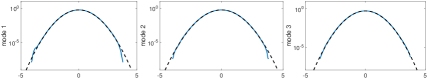
(a)

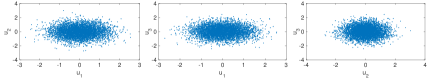
(b) energy equipartition regime

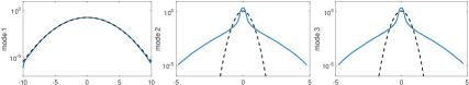
(c)

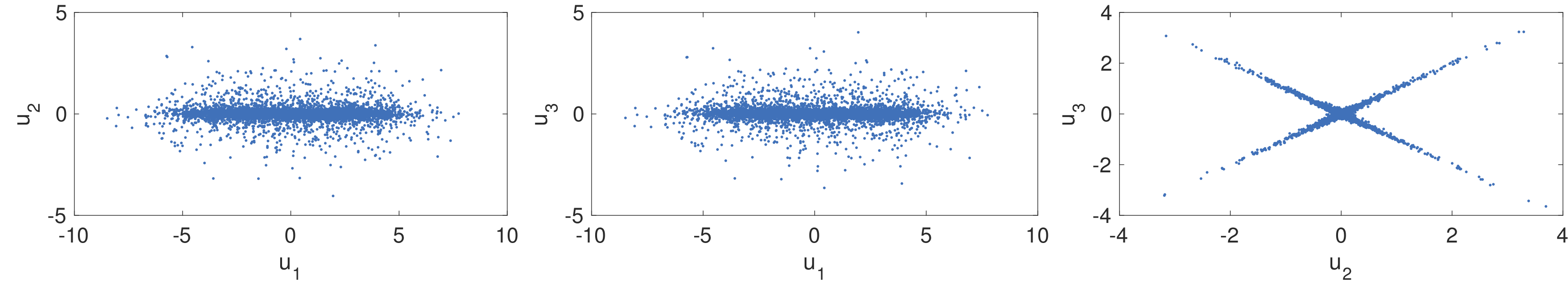
(d) forward energy cascade regime

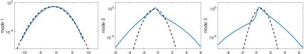
(e)

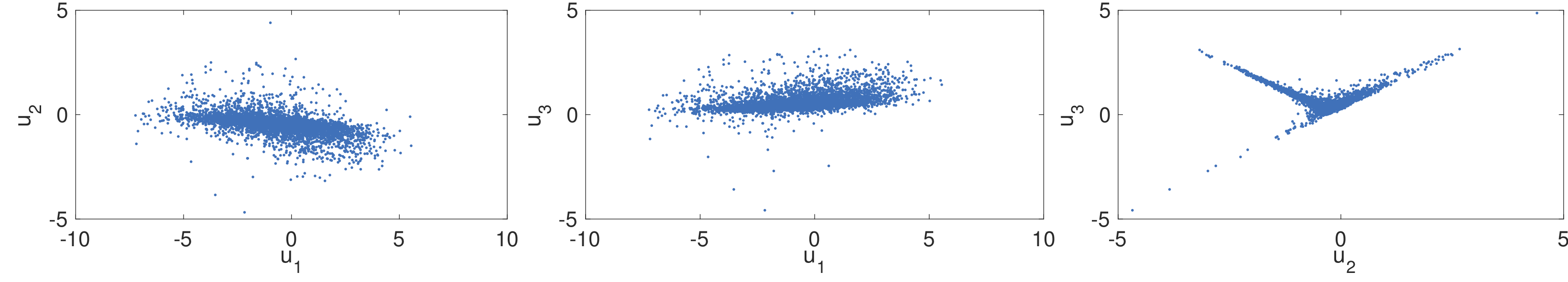
(f) dual energy cascade regime

Figure 4.1: Marginal PDFs in three modes $u_{1},u_{2},u_{3}$ and the joint distributions in scatter plots in three regimes with distinct statistics. Gaussian density functions with the same variance are shown in dashed black lines.

4.3 Reduced-order statistical models for the triad system

In the development about reduced-order models, we focus on the accurate estimation about the first two moments, that is, the statistical mean state and covariance matrix. The major interest is to check the models’ skill in capturing sensitivity in response to external perturbations besides equilibrium consistency in the models. Considering the relatively simple structure in the triad dynamics, we focus on the GC1 and GC2 formulation in (3.4) and (3.5) respectively in the following test cases and the parameter calibration strategy proposed in (3.8). In the model reduction procedure, we first consider the fully resolved model, where the 3-dimensional mean and $3\times 3$ covariance matrix are resolved entirely; and then the diagonal model, where only the mean and diagonal variances are calculated explicitly. In the final step, a severely reduced-order model is introduced where only the variance in the principal mode is resolved.

4.3.1 Reduced model formulation for the triad system (Model selection)

Applying exactly the modeling procedure in Section 3 to the triad system, the two-moment closure schemes replace the higher order moments with additional damping and excitement containing only first two order of moments. The first approach is to run the full system with mean and covariance matrix where both diagonal variances and off-diagonal components are resolved for $\bar{\mathbf{u}}\in\mathbb{R}^{3}$ and $R\in\mathbb{R}^{3\times 3}$

(4.7a) $$\frac{d\bar{\mathbf{u}}}{dt} = L\bar{\mathbf{u}}+B\left(\bar{\mathbf{u}},\bar{\mathbf{u}}\right)+\sum_{i,j}R_{ij}B\left(\mathbf{e}_{i},\mathbf{e}_{j}\right)+\mathbf{F},$$

(4.7b) $$\frac{dR}{dt} = L_{v}\left(\bar{\mathbf{u}}\right)R+RL_{v}^{*}\left(\bar{\mathbf{u}}\right)+Q_{\mathrm{GC}}+Q_{\sigma}.$$

As a test for reduced order methods, we also check the models’ skill by ignoring the cross-covariances. Especially for the triad system, the off-diagonal cross-covariances play a crucial role in the computation of mean and variance responses, while on the other hand, are difficult and expensive to estimate with accuracy. Then the unresolved covariances are approximated from steady state information.

• Fully Resolved Model: In this fully resolved model, the entire mean and covariance matrix are calculated through the dynamical equations (4.7). The nonlinear flux term is approximated by additional damping and additional noise as in (3.4) and (3.5)

  $$Q_{\mathrm{GC}}=-\left(D_{M}R+RD_{M}^{*}\right)+Q_{M}.$$

• Diagonal Model ignoring cross-covariances: In this diagonal model, the cross-covariances between modes are ignored to improve model efficiency. So the covariance matrix is replaced by diagonal matrix $R=\mathrm{diag}\left(r_{k}\right)$. The correction in $Q_{\mathrm{GC}}$ for higher-order moments calibration is kept the same as the full model for GC1 or GC2 respectively. To correct the error due to the neglect of cross-covariances, we add the cross-covariance correction using only steady state information

  $$r_{ij}=\frac{\mathrm{tr}R}{\mathrm{tr}R_{\mathrm{eq}}}\left\langle u_{i}^{\prime}u_{j}^{\prime}\right\rangle_{\mathrm{eq}}.$$

  The diagonal model can be much more efficient compared with the fully resolved model with a model reduction from $O\left(N^{2}\right)$ to $O\left(N\right)$.

Through construction using the unperturbed equilibrium information, climate consistency is guaranteed in both GC1 and GC2 model. In GC1, only constant damping and noise are added to approximate the unresolved higher order moments, while these terms are further corrected with the total variance in GC2. The exponents in the scaling factors are designed to make them consistent in dimension with the estimated third-order statistics. Actually, these scaling factor becomes quite crucial in capturing model responses to perturbations and model performances in transient state.

As a further reduction in the model we consider the two-moment closure methods in reduced order subspace. In this case, we only resolve the variance in the first mode $u_{1}$, and calculate the mean dynamics for all three modes. Then the reduced order model can be expressed as

(4.8a) $$\frac{d\bar{\mathbf{u}}}{dt} = L\bar{\mathbf{u}}+B\left(\bar{\mathbf{u}},\bar{\mathbf{u}}\right)+\sum_{i,j\in\Lambda}C_{ij}^{\mathrm{red}}B\left(\mathbf{e}_{i},\mathbf{e}_{j}\right)+\mathbf{F}+\mathbf{G},$$

(4.8b) $$\frac{dC^{\mathrm{red}}}{dt} = L_{v}^{\mathrm{red}}\left(\bar{\mathbf{u}}\right)C^{\mathrm{red}}+C^{\mathrm{red}}L_{v}^{\mathrm{red}*}\left(\bar{\mathbf{u}}\right)+Q_{\mathrm{GC}}^{\mathrm{red}}+Q_{\sigma}^{\mathrm{red}}.$$

$\Lambda=\left\{1\right\}$ is the index set that includes the resolved modes. Especially with only the leading variance resolved, $C^{\mathrm{red}}=r_{1}=\left\langle u_{1}^{2}\right\rangle$ is only the variance in mode $u_{1}$. The construction about the reduced-order parameters can follow the general strategy in (3.12a) and (3.12b) exactly.

• Reduced Model with only the principal variance resolved: In the variance equation (4.8b), the formulation is similar as before and we only need to constrain the covariance matrix $C^{\mathrm{red}}$ in the resolved subspace with the first mode $u_{1}$ resolved. The additional damping and noise can be applied in the same way as the reduced-model correction as discussed in (3.12). In the mean dynamics, the unresolved second-order moments in $R_{ij}B\left(\mathbf{e}_{i},\mathbf{e}_{j}\right)$ are corrected following (3.13)

  $$G=\frac{\mathrm{tr}R}{\mathrm{tr}R_{\mathrm{eq}}}\sum_{i,j\in\Lambda^{c}}R_{ij}B\left(\mathbf{e}_{i},\mathbf{e}_{j}\right).$$

  The total variance for model sensitivity correction can also be achieved through the approximated statistical energy dynamics as in (3.16)

  $$\frac{dE^{\mathrm{est}}}{dt}=-d_{\mathrm{eff}}E^{\mathrm{est}}+\sum_{i=1}^{3}\left(F_{i}\bar{u}_{i}+\frac{1}{2}\sigma_{i}^{2}\right).$$

  Note that we have calculated the mean in each mode, then the total variance can be calculated through the total statistical energy $\mathrm{tr}R=2E-\sum_{i=1}^{3}\bar{u}_{i}^{2}$. One additional difficulty in the inhomogeneous case is that different damping rates $d_{j}$ are applied to different modes. So we introduce the effective damping rate $d_{\mathrm{eff}}$ through the statistical steady state information as

  $$d_{\mathrm{eff}}=\frac{\sum_{i=1}^{3}\left(F_{i}\bar{u}_{i,\mathrm{eq}}+\frac{1}{2}\sigma_{i}^{2}\right)}{E_{\mathrm{eq}}}.$$

We also list the explicit statistical mean and variance dynamical equations in Appendix B, as well as the explicit statistical energy dynamics to achieve the total variance of the system when only the leading mode is resolved.

4.3.2 Model consistency and tuning parameters in the training phase (Model calibration)

In the model calibration step, we check the imperfect models’ consistency with climatology when no perturbation is applied. As noticed before, the imperfect models’ skill in capturing the right statistics in transient state is crucial for the convergence to the right fixed point in the energy equation. As an example, Figure 4.2 compares the model performances in regimes with dual energy cascade. It can be observed that the statistical steady state mean and variances are recovered with accuracy due to the climate consistent choice of parameters through (3.4) and (3.5), while GC1 lacks the ability to accurately capture the transient state in the beginning due to its lack of sensitivity.

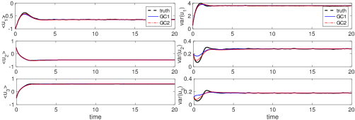
(a) statistics in each mode

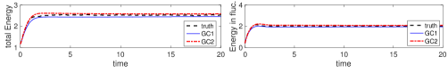
(b) total statistical energy

Figure 4.2: Imperfect model performances in convergence to statistical equilibrium state in dual energy cascade regime. Both GC1 (with constant damping and noise) and GC2 (with correction from total variance) can recover the steady state mean and variance but GC1 lacks the ability to accurately capture the transient state in the beginning due to its lack of sensitivity.

We illustrate the tuning process for optimal model parameters in the training phase in Figure 4.3. Again we use the dual energy cascade regime as an example. Since both the deterministic and stochastic forcing might be perturbed in the external forcing, we consider a kicked response in the initial value according to the perturbation form described in (4.9) and (4.10). In the first row, the information errors with changing model parameter values are shown in total relative entropy from (2.17) as well as the errors in signal and dispersion component. Note that the errors in GC2 model results stay uniformly small in the entire parameter regime, showing the robustness of the method; on the other hand, GC1 model displays larger information error no matter how well we tune the model parameter. This illustrates the inherent information barrier in the closure schemes if we do not consider proper statistical energy scaling in the model damping and noise terms. In the second row, we show the approximation about the linear response operators in the mean and variance using optimal parameters. The transient structures can be captured with accuracy in GC2 model, while GC1 lacks the skill due to the insufficient calibration in the higher-order nonlinear flux approximation.

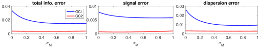
(a) information error with changing parameter values

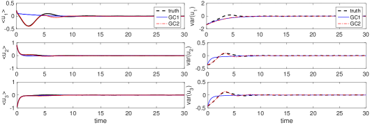
(b) linear responses with optimal parameter

Figure 4.3: Illustration about the training phase for tuning optimal imperfect model parameters for GC1 and GC2. The first row is the information errors with changing values of the tuning parameter $\sigma_{M}$. The second row displays the approximation for the linear response operators in GC1 and GC2 using optimal parameters from the tuning process above.

4.3.3 Model prediction skill to perturbations (Model prediction)

Periodic perturbations added in both deterministic and random forcing are representative in checking the imperfect models’ prediction skill in response to perturbations. The perturbations are introduced in the following forms:

• periodic forcing perturbations in the deterministic forcing: The deterministic forcing perturbation is introduced by a periodic addition to the mean forcing $F=\bar{F}+\delta F$. As one typical test case, we add periodic forcing perturbations $\delta F$ to each mode, that is,

  (4.9) $$\delta F_{i}=A_{i}\sin\left(\omega t\right),$$

  with $\omega$ taking the value $\pi/4$, and $A_{i}$ measures the perturbation amplitude in each mode.

• periodic perturbation in the stochastic random forcing: Also to add stronger time-dependent effect to the variances, we add periodic random forcing to the system by setting

  (4.10) $$\sigma_{j}=\bar{\sigma}_{j}+\delta f^{2}\left(t\right)\left(\sigma_{T_{j}}-\bar{\sigma}_{j}\right),$$

  with $\delta f\left(t\right)=\sin\left(\omega t\right)$ also set to be periodic. Here $\bar{\sigma}_{j}$ is the mean stochastic forcing amplitude in the unperturbed case with $\sigma_{T_{j}}>\bar{\sigma}_{j}$ to add perturbations to this unperturbed mean.

We check the model performances in predicting response to the periodic perturbations in both deterministic and stochastic components. Here we display the imperfect model prediction skill in the toughest regime with dual energy cascade. Thus strong nonlinear coupling is present between the modes. In Figure 4.4, the fully resolved model with mean and $3\times 3$ covariance matrix is applied to the typical regime in GC1 and GC2 closure methods. In this regime with skewed distributions, higher order moments become crucial and need more detailed calibration. As we can see from the results, the deficiency of GC1 method appears in this regime due to the inaccurate approximation about the third-order moments. Large deviation takes place in the skewed modes $u_{2},u_{3}$ due to the errors from third-order energy transfer. In contrast, GC2 model maintains the high skill in predicting the mean and variances with the more careful calibration about the nonlinear flux through the scaling factor using total statistical energy.

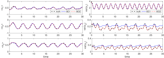
(a)

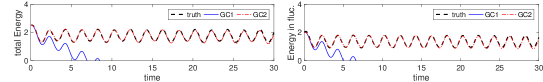
(b)

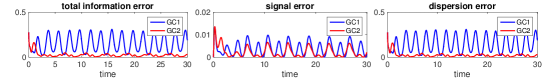
(c)

Figure 4.4: Full GC1 and GC2 model with optimal parameter in approximating responses to periodic external forcing in regimes with dual cascade. The first three rows show the GC1 and GC2 predictions for the statistical mean and variances in each mode together with the truth from MC simulations in thick black lines. The total energy $E$ from the energy equation and the fluctuation energy $E^{\prime}=E-\frac{1}{2}\bar{\mathbf{u}}^{2}$ are compared in the following row. The last line shows the total information error in the imperfect models together with the signal and dispersion components.

In Figure 4.5, we check the diagonal models with only mean and variances in each mode resolved and ignoring the off-diagonal cross-covariances. Like the previous case of full model, GC1 loses the skill in predicting the responses in $u_{2},u_{3}$ due to the lack of information in the third-order interactions. The errors in the beginning transient regime drive the statistical equation to the wrong state or even blowing up. GC2 keeps the skill in capturing the response structures of both the mean and variances. And again most of the error takes place in the variance estimations.

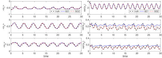
(a)

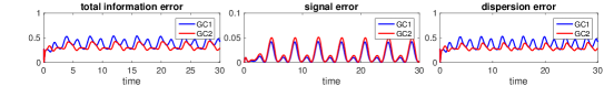
(b)

Figure 4.5: Diagonal GC1 and GC2 model with optimal parameter in approximating responses to periodic external forcing in regimes with dual cascade. The first three rows show the GC1 and GC2 predictions for the statistical mean and variances in each mode together with the truth from MC simulations in thick black lines. The last line shows the total information error in the imperfect models together with the signal and dispersion components.

Testing the feasibility of the reduced-order strategies described previous is important for further applications to general high dimensional turbulent systems because the triad interactions always represent the nonlinear interactions in different scales which usually are ignored in realistic modeling. The same dynamical regime is tested here for the reduced-order models. In this case, only the variance in the first mode $u_{1}$ is resolved explicitly. Especially for this regime with strong dual energy cascade, as we have seen in the true statistical dynamics, strong coupling exists between the high energy mode $u_{1}$ and the less energetic modes, $u_{2},u_{3}$, in both third-order moments and second-order cross-covariances. Thus this becomes a challenging situation for the reduced-order models for capturing the responses with accuracy. The model prediction results are shown in Figure 4.6. With forward and backward energy cascade, strong nonlinear high-order interactions become crucial here. GC1 loses its skill in this case and ends with large errors especially in the mean state $u_{1}$. This is no surprise considering the strong perturbed deviation from the equilibrium state in this regime due to the nonlinear energy transfer while GC1 model only uses unperturbed equilibrium information. On the other hand, GC2 keeps its skill and can capture the responses in both mean and variance with only a single low-order mode resolved.

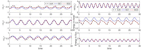
(a)

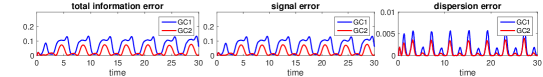
(b)

Figure 4.6: Reduced-order GC1 and GC2 model with the variance in first mode resolved in approximating responses to periodic external forcing in dual energy cascade regime. The first three rows show the GC1 and GC2 predictions for the statistical mean and variances in each mode together with the truth from MC simulations in thick black lines. The last line shows the total information error in the imperfect models together with the signal and dispersion components.

4.3.4 Additional results for the triad model with equipartition of energy

In the final part of this section, we illustrate the imperfect model prediction skills in the equipartition of energy regime with Gaussian statistics. In this case, the three modes $\left(u_{1},u_{2},u_{3}\right)$ in the triad model possess same amount of energy in statistical equilibrium state as in (4.3) and (4.4). In Figure 4.7 and 4.8, we show the prediction results to the periodic perturbations from the diagonal model with off-diagonal cross-covariances neglected, and from the reduced model with only the variance in the first mode $u_{1}$ resolved. Both GC1 and GC2 can capture the mean states in all three modes quite accurately, and GC1 and GC2 results have little difference. This is due to the relatively simple energy mechanism in this regime with same amount of energy in each mode. On the other hand, in the prediction of variances in the diagonal model larger errors appear especially in the modes $u_{2}$ and $u_{3}$. This shows the important effects of the off-diagonal covariances in predicting second order moments in this equipartition energy regime. The reduced model gets good predictions for the variance in the first resolved mode $u_{1}$. With the more expensive full model, the prediction for the variances in all three modes will become accurate with larger computational cost.

(a)

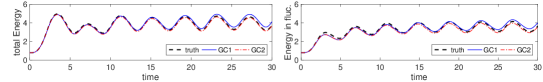
(b)

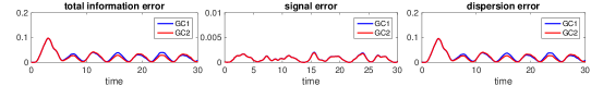
(c)

Figure 4.7: Diagonal GC1 and GC2 model with optimal parameter in approximating responses to periodic external forcing in regimes with equipartition of energy. The first three rows show the GC1 and GC2 predictions for the statistical mean and variances in each mode together with the truth from MC simulations in thick black lines. The total energy $E$ from the energy equation and the fluctuation energy $E^{\prime}=E-\frac{1}{2}\bar{\mathbf{u}}^{2}$ are compared in the following row. The last line shows the total information error in the imperfect models together with the signal and dispersion components.

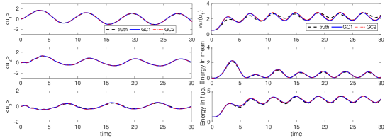
(a)

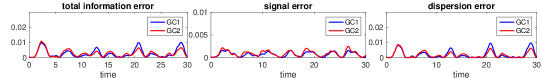
(b)

Figure 4.8: Reduced-order GC1 and GC2 model with the variance in first mode resolved in approximating responses to periodic external forcing in equipartition energy regime.

5 Reduced-Order Statistical Models Applied to Two-Layer Baroclinic Turbulence

In this section, we validate the performance of the reduced-order models by the more complicated two-layer quasi-geostrophic system with baroclinic instability. It is shown that the baroclinic model is capable in capturing the essential physics of the relevant internal variability despite its relatively simple dynamical structure. Two dynamical regimes with typical statistical features are representative in many applications [90, 4, 79]. The first one is the fully turbulent flow with homogeneous statistics as a result of internal baroclinic instability corresponding to the high-latitude ocean and atmosphere; the second one is the anisotropic flow field with strong meandering zonal jets as in the low/mid-latitude regime. Detailed discussions and comparisons of the construction and test about the reduced-order models in various regimes with representative zonal jets and vortices can be found in [79].

The governing two-layer quasi-geostrophic (QG) equations in a barotropic-baroclinic mode formulation for potential vorticity anomalies $\left(q_{\psi},q_{\tau}\right)$ with periodic boundary condition in both $x,y$ directions are [84, 92]

(5.1) $$\frac{\partial q_{\psi}}{\partial t}+J\left(\psi,q_{\psi}\right)+J\left(\tau,q_{\tau}\right)+\beta\frac{\partial\psi}{\partial x}+U\frac{\partial}{\partial x}\Delta\tau =-\frac{\kappa}{2}\Delta\left(\psi-\tau\right)-\nu\Delta^{s}q_{\psi}+\mathcal{F}_{\psi}\left(\mathbf{x},t\right),$$

$$\frac{\partial q_{\tau}}{\partial t}+J\left(\psi,q_{\tau}\right)+J\left(\tau,q_{\psi}\right)+\beta\frac{\partial\tau}{\partial x}+U\frac{\partial}{\partial x}\left(\Delta\psi+k_{d}^{2}\psi\right) =\frac{\kappa}{2}\Delta\left(\psi-\tau\right)-\nu\Delta^{s}q_{\tau}+\mathcal{F}_{\tau}\left(\mathbf{x},t\right).$$

Above $q_{\psi}=\Delta\psi$, $q_{\tau}=\Delta\tau-k_{d}^{2}\tau$ are the disturbance potential vorticities in barotropic and baroclinic mode respectively, while $\psi,\tau$ are the corresponding disturbance barotropic and baroclinic stream functions. The barotropic mode $\psi$ can be viewed as the vertically averaged effect from the flow, and the baroclinic mode $\tau$ is usually related with the thermal effect in heat transport. Besides, $J\left(A,B\right)=A_{x}B_{y}-A_{y}B_{x}$ represents the Jacobian operator. $k_{d}=\sqrt{8}/L_{d}=\left(2f_{0}/NH\right)^{2}$ is the baroclinic deformation wavenumber corresponding to the Rossby radius of deformation $L_{d}$. A large-scale vertical shear $\left(U,-U\right)$ with the same strength and opposite directions is assumed in the background to induce baroclinic instability. In the dissipation operators on the right hand sides of the equations (5.1), besides the hyperviscosity, $\nu\Delta^{s}q_{i}$, we only use Ekman friction, $\kappa\Delta\psi_{2}$, with strength $\kappa$ on the lower layer of the flow.

5.1 Representative dynamical regimes for the two-layer baroclinic turbulence

The two-layer quasi-geostrophic system can display various dynamical regimes with distinct statistical features as the parameters are changed. Parameters for high and low/mid latitude dynamical regimes are shown in Table 1. In numerical simulations, the true statistics are calculated by a pseudo-spectra code by resolving the two-layer equations (5.1) with 128 spectral modes zonally and meridionally, corresponding to $256\times 256\times 2$ grid points in total. In the reduced-order methods, only the large-scale modes $\left|\mathbf{k}\right|\leq 10$ are resolved, which is about 0.15% of the full model resolution.

In the simulations for the unperturbed system in ocean and atmosphere regimes, Figure 5.1 displays the two-layer flow structure in high-latitude ocean regime. The first row is the snapshots of the barotropic and baroclinic vorticity. Homogeneous structure can be observed in both cases while larger scale structures appear in the baroclinic mode. It is important to notice the strong correlation in the coherent structures in the barotropic and baroclinic field, illustrating the strong energy transfer between the two modes. The following part shows time-series of energy in barotropic and baroclinic mode, $-\fint\psi q_{\psi},-\fint\tau q_{\tau}$, as well as the potential energy, $\fint k_{d}^{2}\tau^{2}$, compared with the meridional heat flux, $k_{d}^{2}U\fint\psi_{x}\tau$. In Figure 5.2 the results for the two-layer flow in high-latitude atmosphere regime are compared. One important feature here is the flow field alternating between blocked and unblocked regimes. In the stream functions, it can be observed that in the blocked regime, zonal flow is blocked and the field is restricted at separated regimes, while in the unblocked regime strong zonal flow can be observed. Strong meridional heat flux can be observed in the blocked regime while the flow is in state with lower energy and low heat transfer in the zonal unblocked regime.

In mid/low latitude regimes, both the ocean and atmosphere are distinctly inhomogeneous on large scales. The existence of large-amplitude meandering zonal jets in these regimes suggests the regional metastable equilibria, while the large-scale forced perturbations may lead to regular or irregular fluctuations in some extent. The jet structures are illustrated in more detail in Figure 5.3 for the time-series of the zonally average mean flow, $u=-\partial_{y}\psi$. In this low/mid latitude case, especially for the ocean regime, due to the strong zonal jets in wavenumber $k_{y}=6$, zonal modes with $k_{x}=5,6$ become active due to the nonlinear interactions.

Table 1: Model parameters for ocean and atmosphere dynamical regimes in high and low/mid latitude. $N$ is the model resolution, $\beta,k_{d}$ are the rotation parameter and the deformation frequency, $U$ is the background mean shear flow, $\kappa$ is the Ekman drag in the bottom layer. The last three columns display the unstable waveband from linear analysis. $\left(k_{\min},k_{\max}\right)$ shows the range of unstable wavenumbers; $\sigma_{\mathrm{max}}$ is the largest linear growth rate; and $\left(k_{x},k_{y}\right)_{\mathrm{max}}$ is the position of the mode with maximum growth rate.

regime	$N$	$\beta$	$k_{d}$	$U$	$\kappa$		$\left(k_{\min},k_{\max}\right)$	$\sigma_{\mathrm{max}}$	$\left(k_{x},k_{y}\right)_{\mathrm{max}}$
ocean regime, high lat.	256	10	10	1	9		$\left(2.25,14.61\right)$	0.411	(4, 0)
atmosphere regime, high lat.	256	1	4	0.2	0.2		$\left(1.58,6.78\right)$	0.099	(2, 0)

(a) high-latitude regime

regime	$N$	$\beta$	$k_{d}$	$U$	$\kappa$		$\left(k_{\min},k_{\max}\right)$	$\sigma_{\mathrm{max}}$	$\left(k_{x},k_{y}\right)_{\mathrm{max}}$
ocean regime, low/mid lat.	256	100	10	1	1		$\left(7.14,15.63\right)$	0.104	(2, 8)
atmosphere regime, low/mid lat.	256	2.5	4	0.2	0.05		$\left(2.51,7.06\right)$	0.053	(3, 0)

(b) low/mid-latitude regime

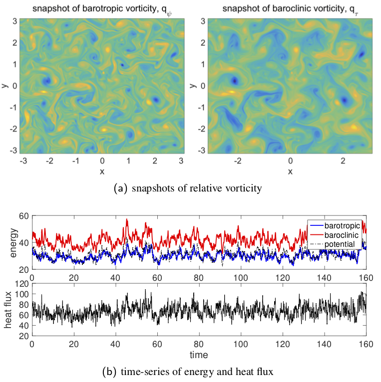
Figure 5.1: Snapshots of high-latitude ocean regime barotropic and baroclinic vorticity in unperturbed system with no external forcing terms. Time-series of energy in barotropic and baroclinic modes, as well as potential energy, are also compared with the heat flux.

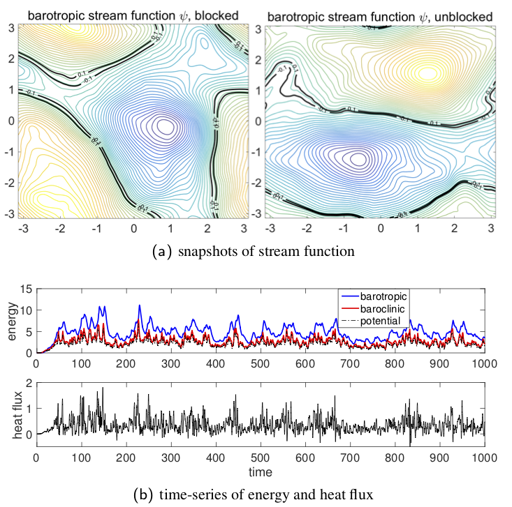
Figure 5.2: Snapshots of high-latitude atmosphere regime barotropic and baroclinic stream function in unperturbed system with no external forcing terms. Time-series of energy in barotropic and baroclinic modes, as well as potential energy, are also compared with the heat flux.

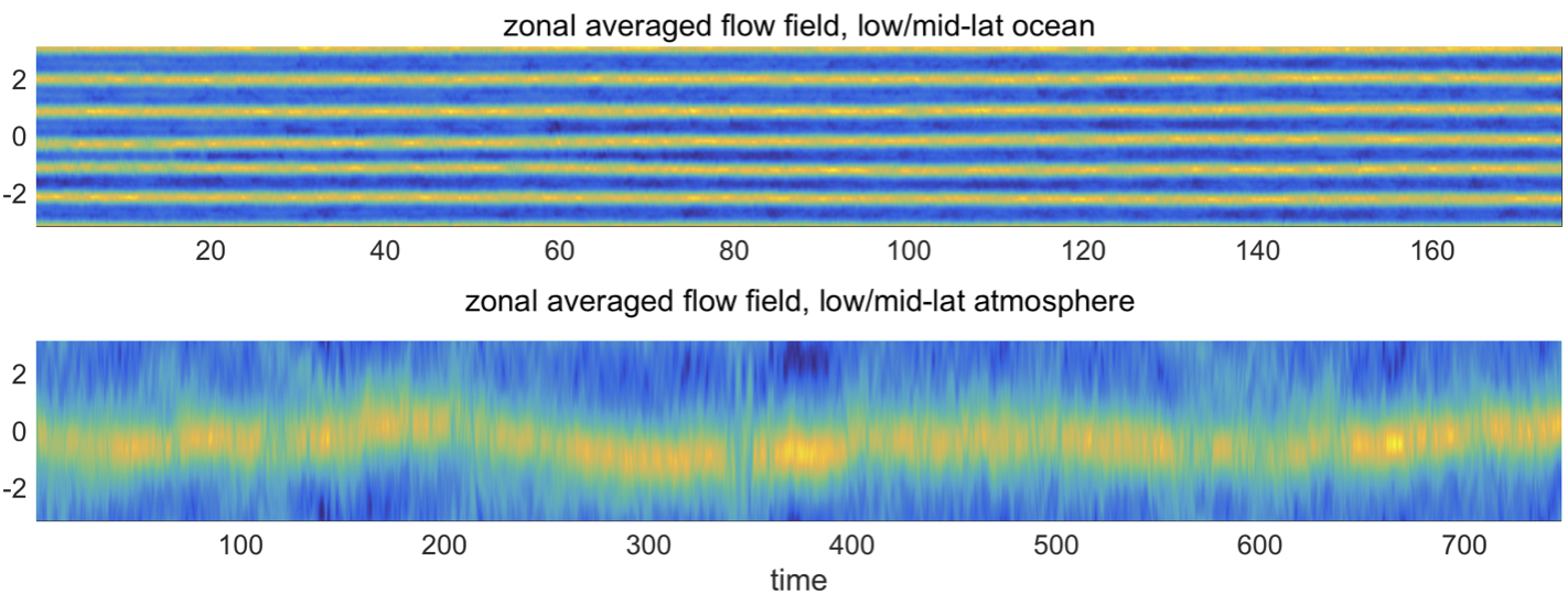
Figure 5.3: Time-series of zonal averaged mean flow with jets in low/mid-latitude atmosphere and ocean regimes.

The general steady state statistical structures in the spectral field are shown in Figure 5.4. As implied from the homogeneous statistics in high-latitude, the mean states stay in small values within fluctuation errors in both ocean and atmosphere regimes. From the energy spectra, one observation is that the potential energy is dominant in large scales in the baroclinic modes, and the kinetic baroclinic energy becomes more important in small scales. For both regimes, we observe wide and energetic spectra that exchange energy between different scales, which indicates strong forward and backward energy cascades along the entire spectral modes.

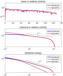
(a) atmosphere regime

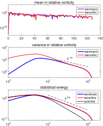
(b) ocean regime

Figure 5.4: Radial-averaged spectra in mean and second-order moments in both atmosphere and ocean high-latitude regimes. The first row compares the statistical mean states (in logarithmic coordinate). The following two rows show the variances, and statistical energy, in barotropic and baroclinic modes, as well as the potential energy.

5.2 Predicting quasi-geostrophic statistical responses in reduced-order models

The quasi-geostrophic response to both stochastic and deterministic perturbations is an important subject in understanding the earth’s atmospheric and oceanic interactions [2, 47]. The same strategy developed in Section 3.3 and applied in the triad system for the first mode in Section 4.3 can be directly generalized to the statistical modeling of the two-layer QG system here.

5.2.1 Statistical formulation about the two-layer baroclinic equations

We formulate the two-layer QG system with Galerkin truncation to finite number of spectral modes. In model simulations, consider a set of rescaled normalized quantities with a high wavenumber truncation $N$ under standard Fourier basis $\mathbf{e_{k}}=\exp\left(i\mathbf{k\cdot x}\right)$ due to the periodic boundary condition, so that

(5.2) $$p_{\psi,\mathbf{k}}= q_{\psi,\mathbf{k}}/\left|\mathbf{k}\right|=-\left|\mathbf{k}\right|\psi_{\mathbf{k}},$$

$$p_{\tau,\mathbf{k}}= q_{\tau,\mathbf{k}}/\sqrt{\left|\mathbf{k}\right|^{2}+k_{d}^{2}}=-\sqrt{\left|\mathbf{k}\right|^{2}+k_{d}^{2}}\tau_{\mathbf{k}}.$$

The introduction of this new set of quantities (5.2) offers convenience that the energy inner-product becomes the standard Euclidean form. Under the above settings, the rescaled set of equations of (5.1) can be summarized in the abstract form in the truncated subspace $\left|\mathbf{k}\right|\leq N$ as in (1.1)

(5.3) $$\frac{d\mathbf{p_{k}}}{dt}=B_{\mathbf{k}}\left(\mathbf{p_{k}},\mathbf{p_{k}}\right)+\left(\mathcal{L}_{\mathbf{k}}-\mathcal{D}_{\mathbf{k}}\right)\mathbf{p_{k}}+\mathcal{F}_{\mathbf{k}},\quad\mathbf{p_{k}}=\left(p_{\psi,\mathbf{k}},p_{\tau,\mathbf{k}}\right)^{T},$$

where the linear operators are decomposed into the non-symmetric part $\mathcal{L}_{\mathbf{k}}$ involving $\beta$-effect and vertical shear flow $U$ and dissipation part $\mathcal{D}_{\mathbf{k}}$, together with the forcing $\mathcal{F}_{\mathbf{k}}$ combining deterministic component and stochastic component compared with (5.1). Most importantly, $B\left(\mathbf{p},\mathbf{p}\right)$ is the nonlinear interactions that conserve both energy and enstrophy.

The same reduced-order modeling strategy then can be applied to the two-layer model following the algorithm in Section 3.4. Therefore the true dynamical equations for the statistical moment $R_{\mathbf{k}}=\left\langle\mathbf{p_{k}}^{*}\mathbf{p_{k}}\right\rangle$ in the form of a $2\times 2$ matrix containing barotropic and baroclinic mode in same wavenumber $\mathbf{k}$ become

(5.4) $$\frac{dR_{\mathbf{k}}}{dt}=\left(\mathcal{L}_{\mathbf{k}}-\mathcal{D}_{\mathbf{k}}\right)R_{\mathbf{k}}+Q_{F,\mathbf{k}}+Q_{\sigma,\mathbf{k}}+c.c.,\quad\left|\mathbf{k}\right|\leq N,$$

where $c.c.$ represent the complex completion for the conjugate parts. On the right hand side of the equation, $\mathcal{L}_{\mathbf{k}},\mathcal{D}_{\mathbf{k}}$ represent the linear interactions between modes, including $\beta$-effect through the rotation of the earth, the effects from the mean shear flow $U$, as well as the dissipations from Ekman drag and hyperviscosity. $Q_{\boldsymbol{\sigma},\mathbf{k}}$ is the external forcing perturbations represented by hypothetical stirring and heating forces. Importantly, the nonlinear flux $Q_{F,\mathbf{k}}$ represents the nonlinear interactions between different wavenumbers due to the advection term. Third-order moments with triad modes $\mathbf{m+n=k}$ enter the first two order moments dynamics representing the nonlinear energy transfer between small and large scales. The nonlinear energy exchange mechanism is crucial in the energy budget, and the conservation property is satisfied due to the triad symmetry as $\sum_{\mathbf{k}}\mathrm{tr}Q_{F,\mathbf{k}}=0$.

5.2.2 Reduced-order model predictions for responses in various dynamical regimes

In constructing the reduced-order models, the same strategy is applied to the crucial but expensive nonlinear flux term $Q_{F}$ as in (3.8)

$$Q_{M,\mathbf{k}}=Q_{M,\mathbf{k}}^{-}+Q_{M,\mathbf{k}}^{+}=f_{1}\left(E\right)\left[-\left(N_{M,\mathbf{k},\mathrm{eq}}+d_{M}\right)R_{M,\mathbf{k}}\right]+f_{2}\left(E\right)\left[Q_{F,\mathbf{k},\mathrm{eq}}^{+}+\sigma_{M,\mathbf{k}}^{2}\right].$$

Both equilibrium higher-order statistics and additional corrections are combined, and statistical energy equation is important to provide the scaling factor for optimal consistency and sensitivity. See [79] for more details.

In checking the model sensitivity in the homogeneous high-latitude regimes, we introduce the forcing perturbation by changing the background jet strength $U$. Note that the deterministic perturbation about zonal mean flow advection forms a difficult test case because the forcing is applied along all wavenumbers with stronger mean-fluctuation interactions involved. On the other hand, for the reduced order methods, only the perturbations at the limited resolved modes are quantified. This gives the inherent difficulty for applying the reduced order models to this kind of perturbations since we have no knowledge of the unresolved modes where large amount of energy is contained. The results with mean flow perturbations $\delta U=\pm 0.05$ in the ocean regime and perturbations $\delta U=0.02,-0.01$ in the atmosphere regime are shown in Figure 5.5 and 5.6 separately. The perturbation accounts for about 5%-10% of the original shear strength $U$, and the corresponding responses in both energy and heat flux spectra are large due to this global perturbation at every wavenumber and nonlinear energy cascade. In the ocean regime, a wide waveband of modes $\left|\mathbf{k}\right|=3,4,5,6$ becomes sensitive to the perturbations; while in the atmosphere regime, the first dominant mode $\left|\mathbf{k}\right|=1$ is especially sensitive to even small perturbations. This illustrates the strong nonlinear interactions between the high and low wavenumber modes. The reduced-order method displays uniform skill in capturing the sensitive responses in the large-scale modes for both positive and negative perturbation cases with only first $10\times 10$ spectral modes resolved compared with the $256\times 256$ full resolution model.

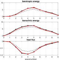
(a) $U=1.05$

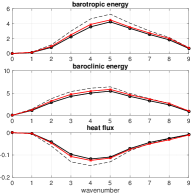
(b) $U=0.95$

Figure 5.5: Reduced-order model predictions to mean shear flow perturbation $\delta U=\pm 0.05$ in high-latitude ocean regime. The reduced-order model predictions for the spectra are compared with the truth. Black lines with circles show the perturbed model responses in the barotropic energy, baroclinic energy, and heat flux. The dashed black lines are the unperturbed statistics, and the reduced order model predictions are in red lines.

(a) $U=0.22$

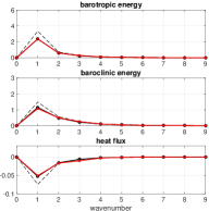
(b) $U=0.19$

Figure 5.6: Reduced-order model predictions to mean shear flow perturbation in high-latitude atmosphere regime. The reduced-order model predictions for the spectra are compared with the truth. Black lines with circles show the perturbed model responses in barotropic energy, baroclinic energy, and heat flux. The dashed black lines are the unperturbed statistics. And the reduced order model predictions are in red lines.

In Figure 5.7 and 5.8, we compare the model responses in both low/mid-latitude ocean and atmosphere regimes. In this inhomogeneous regime with anisotropic jets, the statistical variables combine the responses in the mean and variance, $\overline{p_{1,\mathbf{k}}^{*}p_{2,\mathbf{k}}^{\>}}=\bar{p}_{1,\mathbf{k}}^{*}\bar{p}_{2,\mathbf{k}}^{\>}+\overline{p_{1,\mathbf{k}}^{\prime*}p_{2,\mathbf{k}}^{\prime}}$, to display the total effect from the perturbation. In the ocean regime, the dominant mode with largest sensitivity is at wavenumber $\left|\mathbf{k}\right|=6$ due to the zonal jet structure. The sensitivity is captured with accuracy in the reduced-order method. Also we compare the time evolvement of the total resolved energy and heat flux. The prediction is also good with small error. In the atmosphere regime, $\left|\mathbf{k}\right|=1$ mode gets the largest statistical energy and is most sensitive to perturbations. One important feature is the large change in the heat flux in the first two modes, representing the exchange of energy in the dominant barotropic and baroclinic mode. Still the responses can be captured with accuracy in each mode in the spectra as well as the total energy and heat flux profile with only $10^{2}$ modes resolved. Note that in both cases, the heat flux is weak due to the blocking effect from strong zonal jets.

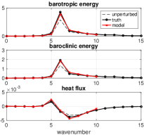
(a)

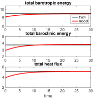
(b)

Figure 5.7: Model responses in low/mid-latitude ocean regime with random forcing perturbation. The left panel shows the spectra for the barotropic and baroclinic energy as well as the heat flux with first ten modes resolved in the reduced-order method. The right panel is the time-series of the total energy and heat flux. The truth is shown in black lines while reduced-order model predictions are in red lines.

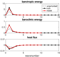
(a)

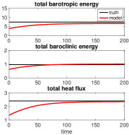
(b)

Figure 5.8: Model responses in low/mid-latitude atmosphere regime with random forcing perturbation. The left panel shows the spectra for the barotropic and baroclinic energy as well as the heat flux with first 10 modes resolved in the reduced-order method. The right panel is the time-series of the total energy and heat flux. The truth is shown in dashed black lines while reduced-order model predictions are in red lines.

6 Summary and Some Future Research Directions

Understanding and improving the predictive skill of imperfect models for high-dimensional complex turbulent systems is a formidable and challenging problem and has been investigated through multiple approaches with various mathematical theories through the years [84, 29, 44, 63, 88, 47]. Low-order truncation methods for statistical prediction can overcome the curse of dimensionality [23, 62] by concentrating on the subspace containing largest variability. On the other hand, anisotropic turbulent processes are representative in many engineering and environmental fluid flows [35, 26] where energy transports intermittently from the smaller scales to impact the largest scales in these flows. Therefore significant model errors always occur due to the high wavenumber truncation in the imperfect model approximations. A systematic information-theoretic framework has been shown useful to improve model fidelity and sensitivity [58, 59, 10] for complex systems including perturbation formulas and multimodel ensembles that can be utilized to improve model error. In many applications to complex systems with model error such as the climate change science [22, 74], it is crucially important to provide guidelines to improve the predictive skill of imperfect models for their responses to changes in various external forcing perturbations.

We discuss the general framework of efficient low-dimensional reduced-order models in this paper for turbulent dynamical systems with nonlinearity to capture statistical responses to external perturbations. The validity of the reduced-order modeling procedure is displayed via the simplest 3-dimensional triad model which is the building block of general turbulent systems, and further on the more complicated two-layer barotropic model with huge model reduction. The computational cost is reduced through a systematic approximation about the expensive nonlinear higher-order interactions. Additional damping and noise corrections are proposed to replace the third-order moments. Model consistency in unperturbed equilibrium and sensitivity to external perturbations are maintained through careful calibration about imperfect model error in a training phase before the prediction. The model errors are calibrated and reduced effectively through a combination of linear response theory involving only unperturbed equilibrium statistics and an information-theoretic framework using information theory. The general framework has been tested in detail for a series of dynamical systems with increasing complexity [63, 78, 79, 54].

For future development about the methods, there exist several interesting and promising directions that are worth further investigation in the next stage:

A)

Tracking the model fluctuation statistics about the perfect statistical mean state. In many problems for turbulent systems, we can assume the statistical mean state is known with reasonable accuracy by averaging along the data trajectory, while the statistical fluctuations about the mean state are the quantities of interest [51, 64]. It is useful to consider accurate and efficient ways to quantify the model fluctuations involving both uncertainties in the perfect system and errors due to imperfect model approximation;

B)

Design of a mitigation control strategy by using novel low-order statistical models. There is need to combine control theory with the statistical model reduction strategies for the principal large-scale modes in the turbulent dynamical systems. For example, it is interesting to consider the effects of climate change using control and statistical modeling strategies;

C)

Predicting passive scalar turbulence with complex flow field. Besides the turbulent flow field, the dynamics of the passive tracer advected by the turbulent flow has many interesting features with practical implications and is worth investigating. One important feature in the turbulent tracer field is the appearance of intermittency despite the near-Gaussian statistics in the background advection flow. The intermittency in time-series and fat-tails in the passive tracer distributions have been observed in nature [73], and have been investigated under a simpler modeling framework both theoretically and numerically [60, 66, 77]. It is thus interesting to consider low-order stochastic and statistical modeling about the tracer field advected by complex turbulent flows;

D)

More detailed consideration about the model nonlinearity. In the reduced-order approximation here, the overall strategy does not require explicit calculation of the inefficient quadratic forms directly, but instead mimic the statistical symmetry in the nonlinearity in simple and efficient forms. Still it is interesting to check the improvement in the low-order models with more detailed approximation.

Appendix A Numerical strategies to calculate the kicked response operators

In the calibration step of the reduced-order models, we use the statistical kicked response theory to tune the imperfect model parameters in the training phase. Here we describe the details about calculating the kicked response operators for the mean and variance numerically. From the formula in (2.10), the response operators for the mean and variance can be achieved from the perturbation part of the probability density $\delta p^{\prime}$. And this density function is also used to measure the information distance between the truth and imperfect model result in the training phase. Below we describe the numerical procedure to get this distribution function $\delta p^{\prime}$ for the true system and the imperfect closure model separately.

• Kicked response for the true model: For the true system, we want to achieve the most accurate possible estimation for the response operators both for comparison with the imperfect model results and for calculating the FDT linear prediction in (2.7). Therefore we use a Monte-Carlo simulation with an large enough ensemble size to capture the response in density. The initial equilibrium ensemble is picked by sampling from a normal distribution with consistent equilibrium mean and variance of the true system. For the kicked response to the mean, a constant perturbation with ten percent of the equilibrium state mean $\delta\mathbf{u}=0.1\bar{\mathbf{u}}_{\mathrm{eq}}$ is added to each initial ensemble member (in fact, as observed in numerical experiments, this perturbation amplitude has little effect on the results in the response distribution as long as it’s not too large); and the initial variance of the ensemble is kept unchanged. The response distribution $\delta p^{\prime}$ then is achieved by monitoring the decay of the ensemble particles back to equilibrium under unperturbed dynamics and uniformly perturbed initial value (and the length of the time window that we need to monitor depends on the mixing property of the turbulent system). See [5, 48] for similar version of this algorithm.

• Kicked response for the imperfect model: For the imperfect model, we just need to run the closure equations to get the responses for the mean and variance. In the same way as the true model, the initial mean is taken from the equilibrium distribution and a perturbation with amplitude $\delta\mathbf{u}=0.1\bar{\mathbf{u}}_{\mathrm{eq}}$ is added to the initial mean state. The initial value for the variance is taken the same as the equilibrium state value and kept unperturbed. Then using this initial mean and variance, the imperfect model with specific closure strategies is applied to monitor the decay of the mean and variance back to equilibrium.

One additional important point that requires attention is that even if the unperturbed equilibrium initial conditions are applied, the system will still deviate from the equilibrium state first and reapproach equilibrium again after some relaxation time. This is due to the insufficient characterization of the entire distribution of the true system with a Gaussian approximation (note that nonlinearities are also included in the imperfect closure methods). To eliminate this effect in computing the kicked response in both the true and imperfect models, we subtract the statistics computed using the unperturbed initial value from the statistics computed using the perturbed Gaussian initial condition to achieve more accurate characterization of the responses.

Appendix B Explicit statistical dynamical formulations for the triad system

We can derive for the triad system (4.1) the dynamical equations for the mean state

(B.1a) $$\frac{d\bar{u}_{1}}{dt} = L_{2}\bar{u}_{3}-L_{3}\bar{u}_{2}-d_{1}\bar{u}_{1}+B_{1}\left(\bar{u}_{2}\bar{u}_{3}+\overline{u_{2}^{\prime}u_{3}^{\prime}}\right)+F_{1},$$

(B.1b) $$\frac{d\bar{u}_{2}}{dt} = L_{3}\bar{u}_{1}-L_{1}\bar{u}_{3}-d_{2}\bar{u}_{2}+B_{2}\left(\bar{u}_{3}\bar{u}_{1}+\overline{u_{3}^{\prime}u_{1}^{\prime}}\right)+F_{2},$$

(B.1c) $$\frac{d\bar{u}_{3}}{dt} = L_{1}\bar{u}_{2}-L_{2}\bar{u}_{1}-d_{3}\bar{u}_{3}+B_{3}\left(\bar{u}_{1}\bar{u}_{2}+\overline{u_{1}^{\prime}u_{2}^{\prime}}\right)+F_{3}.$$

On the right hand sides of the above equations (B.1a)-(B.1c), the first parts include the skew-symmetric interactions between modes as well as the linear damping for the mean. The nonlinear interaction parts enter the mean dynamics both from the interactions between the mean states, and more importantly from the second-order moments of the fluctuations. Thus the mean dynamical equations are not closed by themselves due to the inclusion of unresolved higher-order statistics. Also note that in the second-order moments in the mean equations, diagonal variances won’t appear while the cross-diagonal covariances take place as the role of transferring energy in the mean. Next we consider the dynamics for the fluctuation parts of the state variables

(B.2a) $$\frac{du_{1}^{\prime}}{dt} = L_{2}u_{3}^{\prime}-L_{3}u_{2}^{\prime}-d_{1}u_{1}^{\prime}+B_{1}\left(\bar{u}_{2}u_{3}^{\prime}+u_{2}^{\prime}\bar{u}_{3}+u_{2}^{\prime}u_{3}^{\prime}-\overline{u_{2}^{\prime}u_{3}^{\prime}}\right)+\sigma_{1}\dot{W}_{1},$$

(B.2b) $$\frac{du_{2}^{\prime}}{dt} = L_{3}u_{1}^{\prime}-L_{1}u_{3}^{\prime}-d_{2}u_{2}^{\prime}+B_{2}\left(\bar{u}_{3}u_{1}^{\prime}+u_{3}^{\prime}\bar{u}_{1}+u_{3}^{\prime}u_{1}^{\prime}-\overline{u_{3}^{\prime}u_{1}^{\prime}}\right)+\sigma_{2}\dot{W}_{2},$$

(B.2c) $$\frac{du_{3}^{\prime}}{dt} = L_{1}u_{2}^{\prime}-L_{2}u_{1}^{\prime}-d_{3}u_{3}^{\prime}+B_{3}\left(\bar{u}_{1}u_{2}^{\prime}+u_{1}^{\prime}\bar{u}_{2}+u_{1}^{\prime}u_{2}^{\prime}-\overline{u_{1}^{\prime}u_{2}^{\prime}}\right)+\sigma_{3}\dot{W_{3}}.$$

The above equations can be achieved by subtracting the mean equations from the original triad system. Then the dynamics for higher order moments can be achieved through the fluctuations equations. Importantly, we can get the dynamical equations for the variances in each mode

(B.3a) $$\frac{1}{2}\frac{d\overline{u_{1}^{\prime 2}}}{dt} = L_{2}\overline{u_{1}^{\prime}u_{3}^{\prime}}-L_{3}\overline{u_{1}^{\prime}u_{2}^{\prime}}-d_{1}\overline{u_{1}^{\prime 2}}+B_{1}\left(\bar{u}_{2}\overline{u_{1}^{\prime}u_{3}^{\prime}}+\overline{u_{1}^{\prime}u_{2}^{\prime}}\bar{u}_{3}\right)+B_{1}\overline{u_{1}^{\prime}u_{2}^{\prime}u_{3}^{\prime}}+\frac{1}{2}\sigma_{1}^{2},$$

(B.3b) $$\frac{1}{2}\frac{d\overline{u_{2}^{\prime 2}}}{dt} = L_{3}\overline{u_{1}^{\prime}u_{2}^{\prime}}-L_{1}\overline{u_{2}^{\prime}u_{3}^{\prime}}-d_{2}\overline{u_{2}^{\prime 2}}+B_{2}\left(\bar{u}_{1}\overline{u_{2}^{\prime}u_{3}^{\prime}}+\overline{u_{1}^{\prime}u_{2}^{\prime}}\bar{u}_{3}\right)+B_{2}\overline{u_{1}^{\prime}u_{2}^{\prime}u_{3}^{\prime}}+\frac{1}{2}\sigma_{2}^{2},$$

(B.3c) $$\frac{1}{2}\frac{d\overline{u_{3}^{\prime 2}}}{dt} = L_{1}\overline{u_{2}^{\prime}u_{3}^{\prime}}-L_{2}\overline{u_{1}^{\prime}u_{3}^{\prime}}-d_{3}\overline{u_{3}^{\prime 2}}+B_{3}\left(\bar{u}_{1}\overline{u_{2}^{\prime}u_{3}^{\prime}}+\overline{u_{1}^{\prime}u_{3}^{\prime}}\bar{u}_{2}\right)+B_{3}\overline{u_{1}^{\prime}u_{2}^{\prime}u_{3}^{\prime}}+\frac{1}{2}\sigma_{3}^{2}.$$

And the dynamical equations for the cross-covariances between modes become

(B.4a) $$\frac{d\overline{u_{1}^{\prime}u_{2}^{\prime}}}{dt} = L_{2}\overline{u_{2}^{\prime}u_{3}^{\prime}}-L_{3}\overline{u_{2}^{\prime 2}}-d_{1}\overline{u_{1}^{\prime}u_{2}^{\prime}}+B_{1}\left(\bar{u}_{2}\overline{u_{2}^{\prime}u_{3}^{\prime}}+\overline{u_{2}^{\prime 2}}\bar{u}_{3}\right)+B_{1}\overline{u_{2}^{\prime}u_{2}^{\prime}u_{3}^{\prime}}$$

$$+ L_{3}\overline{u_{1}^{\prime 2}}-L_{1}\overline{u_{1}^{\prime}u_{3}^{\prime}}-d_{2}\overline{u_{1}^{\prime}u_{2}^{\prime}}+B_{2}\left(\bar{u}_{1}\overline{u_{1}^{\prime}u_{3}^{\prime}}+\overline{u_{1}^{\prime 2}}\bar{u}_{3}\right)+B_{2}\overline{u_{1}^{\prime}u_{1}^{\prime}u_{3}^{\prime}},$$

(B.4b) $$\frac{d\overline{u_{1}^{\prime}u_{3}^{\prime}}}{dt} = L_{2}\overline{u_{3}^{\prime 2}}-L_{3}\overline{u_{2}^{\prime}u_{3}^{\prime}}-d_{1}\overline{u_{1}^{\prime}u_{3}^{\prime}}+B_{1}\left(\bar{u}_{2}\overline{u_{3}^{\prime 2}}+\overline{u_{2}^{\prime}u_{3}^{\prime}}\bar{u}_{3}\right)+B_{1}\overline{u_{2}^{\prime}u_{3}^{\prime}u_{3}^{\prime}}$$

$$+ L_{1}\overline{u_{1}^{\prime}u_{2}^{\prime}}-L_{2}\overline{u_{1}^{\prime 2}}-d_{3}\overline{u_{1}^{\prime}u_{3}^{\prime}}+B_{3}\left(\bar{u}_{1}\overline{u_{1}^{\prime}u_{2}^{\prime}}+\overline{u_{1}^{\prime 2}}\bar{u}_{2}\right)+B_{3}\overline{u_{1}^{\prime}u_{1}^{\prime}u_{2}^{\prime}},$$

(B.4c) $$\frac{d\overline{u_{2}^{\prime}u_{3}^{\prime}}}{dt} = L_{3}\overline{u_{1}^{\prime}u_{3}^{\prime}}-L_{1}\overline{u_{3}^{\prime 2}}-d_{2}\overline{u_{2}^{\prime}u_{3}^{\prime}}+B_{2}\left(\bar{u}_{1}\overline{u_{3}^{\prime 2}}+\overline{u_{1}^{\prime}u_{3}^{\prime}}\bar{u}_{3}\right)+B_{2}\overline{u_{1}^{\prime}u_{3}^{\prime}u_{3}^{\prime}}$$

$$+ L_{1}\overline{u_{2}^{\prime 2}}-L_{2}\overline{u_{1}^{\prime}u_{2}^{\prime}}-d_{3}\overline{u_{2}^{\prime}u_{3}^{\prime}}+B_{3}\left(\bar{u}_{1}\overline{u_{2}^{\prime 2}}+\overline{u_{1}^{\prime}u_{2}^{\prime}}\bar{u}_{2}\right)+B_{3}\overline{u_{1}^{\prime}u_{2}^{\prime}u_{2}^{\prime}}.$$

For most situations, it is the diagonal variances in (B.3a)-(B.3c) that we are more interested in, while the off-diagonal covariances (B.4a)-(B.4c) are less important and expensive to resolve. On the other hand, it is noticed that only the cross-covariance terms take place in the central variance dynamics in (B.3a)-(B.3c) for the linear and quasi-linear interaction. In this typical case, if we only consider the diagonal model and ignore the off-diagonal terms in the statistical closure dynamics, huge errors could be introduced in the variance dynamical equations. Thus in the development of reduced order statistical models, careful calibration about the unresolved components becomes crucial in the accuracy of the prediction results.

With the dynamical equations for the mean (B.1) and for the variances in each mode (B.3) and (B.4), we can derive the statistical energy dynamics following the general framework proposed in (2.2) of Theorem 2.1 and also [53]. The statistical energy can be defined as the combination of the mean energy and the fluctuation energy as

$$E=\frac{1}{2}\sum_{i=1}^{3}\left(\bar{u}_{i}^{2}+\overline{u_{i}^{\prime 2}}\right).$$

In the dynamics for the mean and covariance, the major difficulty in resolving the equations explicitly comes from the complex third-order moments in $Q_{F}$ as well as the covariance interactions through $R_{ij}B\left(\mathbf{e}_{i},\mathbf{e}_{j}\right)$. However due to the conservation of energy and the detailed triad symmetry in the triad system, nonlinear interactions cancel in the mean and variance equations and the statistical energy equation becomes

(B.5) $$\frac{dE}{dt}=\frac{d}{dt}\left(\frac{1}{2}\sum_{i=1}^{3}\left(\bar{u}_{i}^{2}+\overline{u_{i}^{\prime 2}}\right)\right)=-\sum_{i=1}^{3}d_{i}\left(\bar{u}_{i}^{2}+\overline{u_{i}^{\prime 2}}\right)+\sum_{i=1}^{3}\left(F_{i}\bar{u}_{i}+\frac{1}{2}\sigma_{i}^{2}\right).$$

Therefore the total statistical structure can be calculated from (B.5) without knowing the higher-order moments as well as cross-covariances which are in general difficult to resolve exactly without error. Furthermore, considering the special case with homogeneous damping in each mode, $d_{j}\equiv d$, the dissipation term on the right hand side of (B.5) becomes $-dE$. Thus we can get the total second-order statistics from only the information in the first-order moments with the help of the statistical energy dynamics.

References

- [1] Rafail V Abramov and Andrew J Majda. Blended response algorithms for linear fluctuation-dissipation for complex nonlinear dynamical systems. Nonlinearity, 20(12):2793–2821, 2007.
- [2] Rafail V Abramov and Andrew J Majda. Low-frequency climate response of quasigeostrophic wind-driven ocean circulation. Journal of Physical Oceanography, 42(2):243–260, 2012.
- [3] Nadine Aubry, Wen-Yu Lian, and Edriss S Titi. Preserving symmetries in the proper orthogonal decomposition. SIAM Journal on Scientific Computing, 14(2):483–505, 1993.
- [4] Nikolaos A Bakas and Petros J Ioannou. Structural stability theory of two-dimensional fluid flow under stochastic forcing. Journal of Fluid Mechanics, 682:332–361, 2011.
- [5] Thomas L Bell. Climate sensitivity from fluctuation dissipation: Some simple model tests. Journal of the Atmospheric Sciences, 37(8):1700–1707, 1980.
- [6] Thomas Bengtsson, Peter Bickel, Bo Li, et al. Curse-of-dimensionality revisited: Collapse of the particle filter in very large scale systems. In Probability and statistics: Essays in honor of David A. Freedman, pages 316–334. Institute of Mathematical Statistics, 2008.
- [7] Michal Branicki, Nan Chen, and Andrew J Majda. Non-Gaussian test models for prediction and state estimation with model errors. Chinese Annals of Mathematics, Series B, 34(1):29–64, 2013.
- [8] Michal Branicki and Andrew J Majda. Quantifying uncertainty for predictions with model error in non-Gaussian systems with intermittency. Nonlinearity, 25(9):2543–2578, 2012.
- [9] Michal Branicki and Andrew J Majda. Fundamental limitations of polynomial chaos for uncertainty quantification in systems with intermittent instabilities. Comm. Math. Sci, 11(1):55–103, 2013.
- [10] Michal Branicki and Andrew J Majda. An information-theoretic framework for improving imperfect dynamical predictions via multi-model ensemble forecasts. Journal of Nonlinear Science, 25(3):489–538, 2015.
- [11] Kenneth P Burnham and David Anderson. Model selection and multi-model inference. A Pratical informatio-theoric approch. Sringer, 2003.
- [12] GF Carnevale, M Falcioni, S Isola, R Purini, and Angelo Vulpiani. Fluctuation-response relations in systems with chaotic behavior. Physics of Fluids A: Fluid Dynamics (1989-1993), 3(9):2247–2254, 1991.
- [13] Abhijit Chatterjee and Dionisios G Vlachos. An overview of spatial microscopic and accelerated kinetic Monte Carlo methods. Journal of computer-aided materials design, 14(2):253–308, 2007.
- [14] N Chen and AJ Majda. Predicting the cloud patterns for the boreal summer intraseasonal oscillation through a low-order stochastic model. Mathematics of Climate and Weather Forecasting, 1(1), 2015.
- [15] N Chen and AJ Majda. Predicting the real-time multivariate madden–julian oscillation index through a low-order nonlinear stochastic model. Monthly Weather Review, 143(6):2148–2169, 2015.
- [16] N Chen, AJ Majda, and D Giannakis. Predicting the cloud patterns of the Madden-Julian oscillation through a low-order nonlinear stochastic model. Geophysical Research Letters, 41:5612–5619, 2014.
- [17] Noel Cressie and Christopher K Wikle. Statistics for spatio-temporal data. John Wiley & Sons, 2015.
- [18] DT Crommelin and AJ Majda. Strategies for model reduction: comparing different optimal bases. Journal of the Atmospheric Sciences, 61(17):2206–2217, 2004.
- [19] Timothy DelSole. Predictability and information theory, volume 1. Center for Ocean-Land-Atmosphere Studies, 2003.
- [20] Timothy DelSole and Jagadish Shukla. Model fidelity versus skill in seasonal forecasting. Journal of Climate, 23(18):4794–4806, 2010.
- [21] Weinan E, JC Mattingly, and Ya Sinai. Gibbsian dynamics and ergodicity for the stochastically forced Navier–Stokes equation. Communications in Mathematical Physics, 224(1):83–106, 2001.
- [22] KA Emanuel, JC Wyngaard, JC McWilliams, DA Randall, and YL Yung. Improving the scientific foundation for atmosphere-land-ocean simulations. Natl. Acad. Press, Washington DC, page 72, 2005.
- [23] Edward S Epstein. Stochastic dynamic prediction. Tellus, 21(6):739–759, 1969.
- [24] Edward S Epstein and Rex J Fleming. Depicting stochastic dynamic forecasts. Journal of the Atmospheric Sciences, 28(4):500–511, 1971.
- [25] Rex J Fleming. On stochastic dynamic prediction. Mon. Wea. Rev, 99:851–872, 1971.
- [26] Uriel Frisch. Turbulence: the legacy of AN Kolmogorov. Cambridge university press, 1995.
- [27] Boris Gershgorin and Andrew J Majda. Quantifying uncertainty for climate change and long-range forecasting scenarios with model errors. Part I: Gaussian models. Journal of Climate, 25(13):4523–4548, 2012.
- [28] Dimitrios Giannakis and Andrew J Majda. Quantifying the predictive skill in long-range forecasting. Part I: Coarse-grained predictions in a simple ocean model. Journal of Climate, 25(6):1793–1813, 2012.
- [29] Dimitrios Giannakis and Andrew J Majda. Quantifying the predictive skill in long-range forecasting. Part II: Model error in coarse-grained Markov models with application to ocean-circulation regimes. Journal of Climate, 25(6):1814–1826, 2012.
- [30] Alexander Gluhovsky and Ernest Agee. An interpretation of atmospheric low-order models. Journal of the atmospheric sciences, 54(6):768–773, 1997.
- [31] Andrey Gritsun and Grant Branstator. Climate response using a three-dimensional operator based on the fluctuation-dissipation theorem. Journal of the atmospheric sciences, 64(7):2558–2575, 2007.
- [32] Andrey Gritsun, Grant Branstator, and Andrew Majda. Climate response of linear and quadratic functionals using the fluctuation-dissipation theorem. Journal of the Atmospheric Sciences, 65(9):2824–2841, 2008.
- [33] Martin Hairer and Andrew J Majda. A simple framework to justify linear response theory. Nonlinearity, 23(4):909, 2010.
- [34] John Harlim, Adam Mahdi, and Andrew J Majda. An ensemble Kalman filter for statistical estimation of physics constrained nonlinear regression models. Journal of Computational Physics, 257:782–812, 2014.
- [35] JO Hinze. Turbulence: An introduction to its mechanisms and theory. Mechanical Engineering, 1959.
- [36] Philip Holmes, John L Lumley, and Gal Berkooz. Turbulence, coherent structures, dynamical systems and symmetry. Cambridge university press, 1998.
- [37] Thomas Y Hou, Wuan Luo, Boris Rozovskii, and Hao-Min Zhou. Wiener chaos expansions and numerical solutions of randomly forced equations of fluid mechanics. Journal of Computational Physics, 216(2):687–706, 2006.
- [38] Edwin T Jaynes. Information theory and statistical mechanics. Physical review, 106(4):620, 1957.
- [39] Markos A Katsoulakis, Andrew J Majda, and Dionisios G Vlachos. Coarse-grained stochastic processes for microscopic lattice systems. Proceedings of the National Academy of Sciences, 100(3):782–787, 2003.
- [40] Richard Kleeman, Andrew J Majda, and Ilya Timofeyev. Quantifying predictability in a model with statistical features of the atmosphere. Proceedings of the National Academy of Sciences, 99(24):15291–15296, 2002.
- [41] Omar M Knio, Habib N Najm, Roger G Ghanem, et al. A stochastic projection method for fluid flow: I. basic formulation. Journal of computational Physics, 173(2):481–511, 2001.
- [42] Solomon Kullback and Richard A Leibler. On information and sufficiency. The annals of mathematical statistics, pages 79–86, 1951.
- [43] CE Leith. Climate response and fluctuation dissipation. Journal of the Atmospheric Sciences, 32(10):2022–2026, 1975.
- [44] Marcel Lesieur. Turbulence in fluids, volume 40. Springer Science & Business Media, 2012.
- [45] Edward N Lorenz. Deterministic nonperiodic flow. Journal of the atmospheric sciences, 20(2):130–141, 1963.
- [46] Edward N Lorenz. Predictability: A problem partly solved. In Proc. Seminar on predictability, volume 1, 1996.
- [47] Nicholas J Lutsko, Isaac M Held, and Pablo Zurita-Gotor. Applying the fluctuation–dissipation theorem to a two-layer model of quasigeostrophic turbulence. Journal of the Atmospheric Sciences, 72(8):3161–3177, 2015.
- [48] Andrew Majda, Rafail V Abramov, and Marcus J Grote. Information theory and stochastics for multiscale nonlinear systems, volume 25. American Mathematical Soc., 2005.
- [49] Andrew Majda, Richard Kleeman, and David Cai. A mathematical framework for quantifying predictability through relative entropy. Methods and Applications of Analysis, 9(3):425–444, 2002.
- [50] Andrew Majda, Ilya Timofeyev, and Eric Vanden-Eijnden. A priori tests of a stochastic mode reduction strategy. Physica D: Nonlinear Phenomena, 170(3):206–252, 2002.
- [51] Andrew Majda and Xiaoming Wang. Nonlinear dynamics and statistical theories for basic geophysical flows. Cambridge University Press, 2006.
- [52] Andrew Majda and Xiaoming Wang. Linear response theory for statistical ensembles in complex systems with time-periodic forcing. Communications in Mathematical Sciences, 8(1):145–172, 2010.
- [53] Andrew J Majda. Statistical energy conservation principle for inhomogeneous turbulent dynamical systems. Proceedings of the National Academy of Sciences, 112(29):8937–8941, 2015.
- [54] Andrew J Majda. Introduction to turbulent dynamical systems in complex systems. Springer, 2016.
- [55] Andrew J Majda, Rafail Abramov, and Boris Gershgorin. High skill in low-frequency climate response through fluctuation dissipation theorems despite structural instability. Proceedings of the National Academy of Sciences, 107(2):581–586, 2010.
- [56] Andrew J Majda and Michal Branicki. Lessons in uncertainty quantification for turbulent dynamical systems. Discrete Cont. Dyn. Systems, 32(9):3133–3221, 2012.
- [57] Andrew J Majda and Boris Gershgorin. Quantifying uncertainty in climate change science through empirical information theory. Proceedings of the National Academy of Sciences, 107(34):14958–14963, 2010.
- [58] Andrew J Majda and Boris Gershgorin. Improving model fidelity and sensitivity for complex systems through empirical information theory. Proceedings of the National Academy of Sciences, 108(25):10044–10049, 2011.
- [59] Andrew J Majda and Boris Gershgorin. Link between statistical equilibrium fidelity and forecasting skill for complex systems with model error. Proceedings of the National Academy of Sciences, 108(31):12599–12604, 2011.
- [60] Andrew J Majda and Boris Gershgorin. Elementary models for turbulent diffusion with complex physical features: eddy diffusivity, spectrum and intermittency. Phil. Trans. R. Soc. A, 371: 20120184, 2013.
- [61] Andrew J Majda, Boris Gershgorin, and Yuan Yuan. Low-frequency climate response and fluctuation-dissipation theorems: theory and practice. Journal of the Atmospheric Sciences, 67(4):1186–1201, 2010.
- [62] Andrew J Majda and John Harlim. Physics constrained nonlinear regression models for time series. Nonlinearity, 26(1):201–217, 2012.
- [63] Andrew J Majda and Di Qi. Improving prediction skill of imperfect turbulent models through statistical response and information theory. Journal of Nonlinear Science, 26(1):233–285, 2016.
- [64] Andrew J Majda, Ilya Timofeyev, and Eric Vanden-Eijnden. Systematic strategies for stochastic mode reduction in climate. Journal of the Atmospheric Sciences, 60(14):1705–1722, 2003.
- [65] Andrew J Majda and Xin T Tong. Ergodicity of truncated stochastic Navier-Stokes with deterministic forcing and dispersion. Journal of Nonlinear Science, 26(5):1483–1506, 2015.
- [66] Andrew J Majda and Xin T Tong. Intermittency in turbulent diffusion models with a mean gradient. Nonlinearity, 28(11):4171–4208, 2015.
- [67] Andrew J Majda and Yuan Yuan. Fundamental limitations of ad hoc linear and quadratic multi-level regression models for physical systems. Discrete and Continuous Dynamical Systems B, 17(4):1333–1363, 2012.
- [68] Umberto Marini Bettolo Marconi, Andrea Puglisi, Lamberto Rondoni, and Angelo Vulpiani. Fluctuation–dissipation: response theory in statistical physics. Physics reports, 461(4):111–195, 2008.
- [69] Henry P McKean. A class of markov processes associated with nonlinear parabolic equations. Proceedings of the National Academy of Sciences, 56(6):1907–1911, 1966.
- [70] Mustafa A Mohamad, Will Cousins, and Themistoklis P Sapsis. A probabilistic decomposition-synthesis method for the quantification of rare events due to internal instabilities. arXiv preprint arXiv:1511.02392, 2015.
- [71] Mustafa A Mohamad and Themistoklis P Sapsis. Probabilistic response and rare events in mathieu׳ s equation under correlated parametric excitation. Ocean Engineering, 120:289–297, 2016.
- [72] Habib N Najm. Uncertainty quantification and polynomial chaos techniques in computational fluid dynamics. Annual Review of Fluid Mechanics, 41:35–52, 2009.
- [73] J David Neelin, Benjamin R Lintner, Baijun Tian, Qinbin Li, Li Zhang, Prabir K Patra, Moustafa T Chahine, and Samuel N Stechmann. Long tails in deep columns of natural and anthropogenic tropospheric tracers. Geophysical Research Letters, 37(5), 2010.
- [74] J David Neelin, Matthias Münnich, Hui Su, Joyce E Meyerson, and Christopher E Holloway. Tropical drying trends in global warming models and observations. Proceedings of the National Academy of Sciences, 103(16):6110–6115, 2006.
- [75] Dwight Roy Nicholson. Introduction to plasma theory. Cambridge Univ Press, 1983.
- [76] Stephen B Pope. Turbulent flows. IOP Publishing, Bristol, 2001.
- [77] Di Qi and Andrew J Majda. Predicting fat-tailed intermittent probability distributions in passive scalar turbulence with imperfect models through empirical information theory. Comm. Math. Sci, 14(6):1687–1722, 2015.
- [78] Di Qi and Andrew J Majda. Low-dimensional reduced-order models for statistical response and uncertainty quantification: barotropic turbulence with topography. Physica D: Nonlinear Phenomena, http://dx.doi.org/10.1016/j.physd.2016.11.006, 2016.
- [79] Di Qi and Andrew J Majda. Low-dimensional reduced-order models for statistical response and uncertainty quantification: two-layer baroclinic turbulence. Journal of the Atmospheric Sciences, 73(12):4609–4639, 2016.
- [80] David A Randall, Richard A Wood, Sandrine Bony, Robert Colman, Thierry Fichefet, John Fyfe, Vladimir Kattsov, Andrew Pitman, Jagadish Shukla, Jayaraman Srinivasan, et al. Climate models and their evaluation. In Climate change 2007: The physical science basis. Contribution of Working Group I to the Fourth Assessment Report of the IPCC (FAR), pages 589–662. Cambridge University Press, 2007.
- [81] Aaditya V Rangan, Louis Tao, Gregor Kovacic, and David Cai. Multiscale modeling of the primary visual cortex. IEEE Engineering in Medicine and Biology Magazine, 28(3):19–24, 2009.
- [82] James C Robinson. Infinite-dimensional dynamical systems: an introduction to dissipative parabolic PDEs and the theory of global attractors, volume 28. Cambridge University Press, 2001.
- [83] David Ruelle. Differentiation of SRB states. Communications in Mathematical Physics, 187(1):227–241, 1997.
- [84] Rick Salmon. Lectures on geophysical fluid dynamics. Oxford University Press, 1998.
- [85] Themistoklis P Sapsis. Attractor local dimensionality, nonlinear energy transfers and finite-time instabilities in unstable dynamical systems with applications to two-dimensional fluid flows. In Proc. R. Soc. A, volume 469, page 20120550. The Royal Society, 2013.
- [86] Themistoklis P Sapsis and Pierre FJ Lermusiaux. Dynamically orthogonal field equations for continuous stochastic dynamical systems. Physica D: Nonlinear Phenomena, 238(23):2347–2360, 2009.
- [87] Themistoklis P Sapsis and Andrew J Majda. Blended reduced subspace algorithms for uncertainty quantification of quadratic systems with a stable mean state. Physica D: Nonlinear Phenomena, 258:61–76, 2013.
- [88] Themistoklis P Sapsis and Andrew J Majda. Statistically accurate low-order models for uncertainty quantification in turbulent dynamical systems. Proceedings of the National Academy of Sciences, 110(34):13705–13710, 2013.
- [89] Themistoklis P Sapsis and Andrew J Majda. A statistically accurate modified quasilinear Gaussian closure for uncertainty quantification in turbulent dynamical systems. Physica D: Nonlinear Phenomena, 252:34–45, 2013.
- [90] Kaushik Srinivasan and WR Young. Zonostrophic instability. Journal of the atmospheric sciences, 69(5):1633–1656, 2012.
- [91] Albert A Townsend. The structure of turbulent shear flow. Cambridge university press, 1980.
- [92] Geoffrey K Vallis. Atmospheric and oceanic fluid dynamics: Fundamentals and large-scale circulation. Cambridge University Press, 2006.
- [93] Lai-Sang Young. What are SRB measures, and which dynamical systems have them? Journal of Statistical Physics, 108(5):733–754, 2002.