Renormalization Group Flow of the Aharonov-Bohm Scattering Amplitude

Abstract

The Aharonov-Bohm elastic scattering with incident particles described by plane waves is revisited by using the phase-shifts method. The formal equivalence between the cylindrical Schrödinger equation and the one-dimensional Calogero problem allows us to show that up to two scattering phase-shifts modes in the cylindrical waves expansion must be renormalized. The renormalization procedure introduces new length scales giving rise to spontaneous breaking of the conformal symmetry. The new renormalized cross-section has an amazing property of being non-vanishing even for a quantized magnetic flux, coinciding with the case of Dirac delta function potential. The knowledge of the exact beta function permits us to describe the renormalization group flows within the two-parametric family of renormalized Aharonov-Bohm scattering amplitudes. Our analysis demonstrates that for quantized magnetic fluxes a BKT-like phase transition at the coupling space occurs.

1 Introduction

In the presence of an external electromagnetic field, the wave function of a charged particle in quantum mechanics contains a non-integrable phase factor, which is responsible for observable quantum effects in the case of non-simply connected spaces. The most representative example of such phenomenon is the famous Aharonov-Bohm (AB) magnetic effect [3], experimentally confirmed in ref. [4]. It has provided also important insights for generalizations to the case of non-abelian gauge fields, where the analogous phase factor turns out to play a relevant role even for simply-connected spaces [5].

The present article is dedicated to the rigorous study of two long-standing problems of the original AB elastic scattering for non-relativistic spinless incident particle with well defined momentum, i.e. the plane wave. Since the minimal coupling introduces a non-integrable phase in the incident plane wave, related to the magnetic flux $\Phi$, the usual scattering boundary condition cannot be trivially implemented, due to the apparent multivaluedness of the wave function. In the first part of the paper we review the exact phase-shift method, where the problematic phase is transferred to the outgoing cylindrical wave, that allows to derive the AB scattering amplitude in a rather simple way [7]. This approach however introduces an unexpected “side effect”, namely an extra $\delta$-function term in the scattering amplitude, that will be discussed in Sect. 2. Within the framework of this method, the total wave function is realized as a superposition of cylindrical waves of different angular momenta $m=0,\pm 1,\pm 2,...$, each one of them obeying a Dirichlet boundary condition (b.c.) at the origin. The development of modern mathematical tools for self-adjoint (s.a.) extensions of second order differential operators [8], as the one given by the cylindrical AB Hamiltonian $H_{cal}=-\frac{d^{2}}{dr^{2}}+V(r)$, pointed out that the above statement fails to be valid for certain range of values of the effective coupling constant $\mathcal{C}_{m}=(m+\alpha)^{2}<\frac{3}{4}$ of the Calogero potential $V(r)=\mathcal{C}_{m}/r^{2}$. The correct implementation of the s.a. condition for the AB operator $H_{cal}$ requires the consideration of a one-parametric family of more general Dirichlet or mixed b.c.’s for the corresponding AB cylindrical wave functions. Although this problem and its mathematical solution have already been widely discussed in the literature [8, 9, 10], their implications for AB scattering amplitudes are not yet completely explored and far from being fully understood.

The second part of the paper represents an attempt for a complete description of all the physical consequences coming from the correct s.a. extension of the cylindrical AB Hamiltonian. In section 3, by taking into account the correspondence of the AB cylindrical equation with the one dimensional Calogero problem [11, 12], we solve the b.c. problem by using the renormalization method of Beane et al. [9]. As a result of this renormalization the scattering amplitude acquires up to two new scale parameters, characterizing the conformal symmetry breaking and thus providing an example of dimensional transmutation [13]. It also introduces certain important corrections to the original AB cross-section. The most impressive result of this renormalization procedure is the prediction of the explicit form of a nontrivial isotropic cross-section in the case of “quantized” magnetic flux $\Phi=n\Phi_{0}$. In the final part of section 3 the conditions for the existence of a few bound states consistent with the AB scattering problem are explored. They can be considered as the remnants of the Landau levels that have survived after the zero radius limit of the AB solenoid. The exact beta function of the running coupling and related RG flows are studied in details in section 4. Again, the case of quantized magnetic flux exhibits particularly interesting features: only one mode needs to be renormalized and the two RG fixed points in the coupling space collide into a BKT-like critical point of an infinite order phase transition [14, 15, 16]. A discussion about the physical meaning of the new quantum scales is presented at our concluding section 5.

2 AB scattering on infinitely thin solenoid

The original AB effect concerns a scattering process involving a charged particle and an infinite ideal solenoid. The solenoid is placed along the $z$-axis and has a small radius $r_{c}$ and a strong magnetic field $\vec{B}=B\hat{z}$. The limits $r_{c}\rightarrow 0$ and $B\rightarrow\infty$ are taken by keeping the magnetic flux $\Phi=\pi r_{c}^{2}B$ fixed and finite. We will use the term “infinitely thin solenoid” for this configuration [8]. In the plane ortogonal to the solenoid there is no magnetic field at any point, except for the origin of the coordinate system. The standard gauge choice given by $\vec{A}=\frac{\Phi}{2\pi}\frac{\hat{\varphi}}{r}$, $r=\sqrt{x^{2}+y^{2}}\neq 0$ provides $\oint_{C}\vec{A}.d\vec{l}=\Phi$ and $\vec{B}=\vec{\nabla}\times\vec{A}=\Phi\delta(x)\delta(y)\hat{z}$. Then the stationary Schrödinger equation describing a spinless particle with mass $M$ and electric charge $-|e|$ interacting with the infinitely thin solenoid takes the form:

$$-\frac{\hbar^{2}}{2M}\left(\vec{\nabla}+i\frac{|e|}{\hbar}\vec{A}\right)^{2}\psi=E\psi.$$ (1)

We consider the general solution for zero momentum $p_{z}=0$, that can be decomposed into a superposition of cylindrical waves in the $x-y$ plane:

$$\phi(r,\varphi)=\sum_{m=-\infty}^{\infty}R_{m}(r)e^{im\varphi},\ r=\sqrt{x^{2}+y^{2}},\ \tan\varphi=y/x.$$ (2)

The functions $R_{m}(r)$ are solutions of the cylindrical Schrödinger equation

$$r^{2}R^{\prime\prime}_{m}(r)+rR^{\prime}_{m}(r)+\left[(kr)^{2}-\left(m+\frac{\Phi}{\Phi_{0}}\right)^{2}\right]R_{m}(r)=0,$$ (3)

which can be solved in terms of Bessel functions [17]

$$R_{m}(r)=A_{m}J_{\nu_{m}}(kr)+B_{m}N_{\nu_{m}}(kr),\ \nu_{m}=\left|m-\alpha\right|,$$ (4)

where $\alpha=\Phi/\Phi_{0}$, $\Phi_{0}\equiv 2\pi\hbar/|e|$.

The gradient form of the vector potential $\vec{A}=\vec{\nabla}\omega(\varphi)$, $\omega(\varphi)=-\alpha\frac{\Phi_{0}}{2\pi}(\pi-\varphi)$, indicates that apparently it represents a pure gauge field configuration. This assertion is not however true since the phase factor $e^{-i\frac{|e|}{\hbar}\omega(\varphi)}$ is a multiple-valued function, $\omega(2\pi)-\omega(0)=\alpha\Phi_{0}$, if $\alpha\Phi_{0}/2\pi\notin\,\mathbb{N}$. Notice that the free particle wave function also shares the same property due to the minimal coupling with the vector potential. Then

$$\psi_{in}^{AB}(r,\varphi)=e^{ikx+i\alpha\left(\pi-\varphi\right)},\ x=r\cos\varphi,$$ (5)

has a branch cut along the positive $x$-axis, $\psi^{AB}_{in}(r,2\pi)/\psi^{AB}_{in}(r,0)=e^{-2i\pi\alpha}$, excepts the special case $\alpha\in\mathbb{N}$ when the magnetic flux has discrete values.

2.1 On the choice of scattering boundary conditions

According to the prescription of the original AB paper, the function $\psi^{AB}_{in}(r,\varphi)$ must be given by the asymptotic form of the incident wave function, in order to ensure that the current density

$$\vec{j}_{in}^{AB}=-i\frac{\hbar}{2M}\left[(\psi_{in}^{AB})^{*}\left(\vec{\nabla}-i\frac{e}{\hbar}\vec{A}\right)\psi_{in}^{AB}-\psi_{in}^{AB}\left(\vec{\nabla}+i\frac{e}{\hbar}\vec{A}\right)(\psi_{in}^{AB})^{*}\right]=\frac{\hbar k}{M}\hat{x},$$ (6)

is a constant along the $x$ direction. Notice that the b.c.

$$\psi^{AB}(r,\phi)\approx e^{ikx+i\alpha\left(\pi-\varphi\right)}+f_{k}^{AB}(\varphi)\frac{e^{ikr}}{\sqrt{-ir}},\ kr\gg 1,$$ (7)

imposed in the original description of the AB scattering, does not correspond to the standard asymptotic form for a short-range interaction elastic scattering, as explained in A (see Eq. (67)). It is usually argued [3] that the multi-valuedness of the incident wave function is expected to be canceled by an equivalent hidden term in the second function representing the cylindrical wave. Aharanov and Bohm have proposed a single-valued ansatz, but the asymptotic expression they have obtained, due to the approximations performed during the calculations, is given by an exponential multi-valued function with a branch-cut along the $x>0$ semi-axis. Only in a few special cases, viz. for $\alpha=n$ and $\alpha=n+1/2$, $n\in\mathbb{N}$, the authors obtain asymptotically single-valued forms.

Our approach to the AB problem is based on a slight modification of the original scattering ansatz, by transferring the extra phase in $\psi_{in}^{AB}$ from the incident wave to the outgoing cylindrical one. The exponential (5) describes a particle which is not interacting with the magnetic field, so locally we have a pure gauge phase. However the fact that $e^{i\alpha(\pi-\varphi)}$ is multi-valued ($\alpha\notin\mathbb{N}$) points out that such a description cannot be adopted over the whole plane. In the scattering process, the incident particle is released from $r\rightarrow\infty$ with $\varphi=\pi$, $\psi_{in}=\psi_{in}^{AB}(x,0)=e^{ikx}$, and goes to the $r\rightarrow\infty$ with $\varphi\rightarrow 0$ or $2\pi$ after scattering. During the scattering, the particle interacts with the solenoid’s magnetic field, so that its wave function cannot be written in the form $\psi_{in}^{AB}$ anymore. Now observe that the AB incident wave can be rewritten as

$$\psi_{in}^{AB}=e^{ikx+i\alpha\left(\pi-\varphi\right)}=e^{ikx}+2ie^{i\frac{\alpha}{2}\left(\pi-\varphi\right)}\sin\left(\frac{\alpha}{2}\left(\pi-\varphi\right)\right)e^{ikx},$$ (8)

thus separating the standard incident wave $e^{ikx}$ from the multi-valued term. Since we are dealing with an elastic scattering from a short range interaction, the scattered wave function $\psi_{scat}$, by definition corresponds to the difference $\psi(r,\varphi)-\psi_{in}(r,\varphi)$, with $r\rightarrow\infty$, $\forall$ $\varphi$. It is therefore natural to interpret the second term of (8) as a part of $\psi_{scat}$. Then assuming that $\psi_{in}=e^{ikx}$, the proper scattering b.c. is now given by equation (67). There is no inconsistency with the probability current density, since the $\vec{j}_{in}=\frac{\hbar k}{M}\hat{x}+\mathcal{O}(1/r)$ continues to be a constant in the limit $r\rightarrow\infty$.

2.2 Exact Scattering Amplitude

Our goal is to derive the exact form of the first (non-renormalized) version of the scattering amplitude, by performing an explicit calculation within the phase-shifts method presented in A and using Eq. (67), i.e.

$$\psi(r,\varphi)\approx e^{ikx}+f_{k}(\varphi)\frac{e^{ikr}}{\sqrt{-ir}},\ x=r\cos\varphi,\ kr\gg 1.$$

as a boundary condition. The normalization coefficient of the solutions of the cylindrical equation (3) and of the phase-shifts are determined by the solution (4) in the limit $kr\gg 1$ corresponding to the specific choice $B_{m}=0$,

$$R_{m}(r) \approx A_{m}\sqrt{\frac{2}{kr}}\sin\left(kr+\frac{\pi}{4}-\frac{\pi}{2}\nu_{m}\right),$$ (9)

$$= A_{m}\sqrt{\frac{2}{kr}}\sin\left(kr-\frac{\pi}{2}\left(m-\frac{1}{2}\right)+\left(m-\frac{\pi}{2}\nu_{m}\right)\right).$$

Comparing with Eq. (69) we see that $Q_{m}(r)=J_{\nu_{m}}(kr)$, i.e. $A_{m}=1$, and

$$\delta_{m}=\frac{\pi}{2}\left(m-\nu_{m}\right).$$ (10)

It is worthwhile to mention that the presence of the magnetic field breaks down the symmetry $\delta_{m}=\delta_{-m}$, that is usually manifest in the case of central forces. Replacing the formula above in Eq. (68) completely determines the exact and single-valued form of the total wave function:

$$\psi(r,\varphi)=\sum_{m=-\infty}^{\infty}(-1)^{m}(-i)^{\nu_{m}}J_{\nu_{m}}(kr).$$ (11)

This result turns out to be different from the original AB ansatz by a factor of $(-1)^{m}$ and it perfectly agrees with the wave function obtained in ref. [19] by two different methods. By construction, the wave function has the plane wave $e^{ikx}$ as a limit when $\nu_{m}\rightarrow|m|$, which is given by the equation (70). To make the calculations clearer we will introduce a new definition for the magnetic flux, $\Phi/\Phi_{0}\equiv\alpha=n+\zeta$, where $n\in\mathbb{N}$ and $0\leq\zeta<1$. In this notation we have

$$\delta_{m}=\left\{\begin{array}[]{ll}-\frac{\pi n}{2}-\frac{\pi}{2}\zeta,\ m+n+\zeta\geq 0,\\ \pi m+\frac{\pi n}{2}+\frac{\pi}{2}\zeta,\ m+n+\zeta<0.\end{array}\right.$$ (14)

The phase-shifts given by Eq. (71), together with the redefinition $m\rightarrow m-n$, gives

$$f_{k}(\varphi) = e^{-in\varphi}\frac{1}{i\sqrt{2\pi k}}\sum_{m=-\infty}^{\infty}\left(e^{2i\delta_{m-n}}-1\right)e^{im\varphi},$$ (15)

$$= e^{-in\varphi}\frac{1}{i\sqrt{2\pi k}}\left(\sum_{m=0}^{\infty}\left(e^{-in\pi}e^{-i\pi\zeta}-1\right)e^{im\varphi}+\sum_{m=1}^{\infty}\left(e^{-in\pi}e^{i\pi\zeta}-1\right)e^{-im\varphi}\right),$$

$$= -e^{-in\varphi}\frac{2}{\sqrt{2\pi k}}\Bigg{(}e^{-i\frac{\pi}{2}(n+\zeta)}\sin\left(\frac{\pi}{2}(n+\zeta)\right)\sum_{m=0}^{\infty}e^{im\varphi}$$

$$+e^{-i\frac{\pi}{2}(n-\zeta)}\sin\left(\frac{\pi}{2}(n-\zeta)\right)\sum_{m=1}^{\infty}e^{-im\varphi}\Bigg{)}.$$

The above geometric progression series cannot be performed directly, however. First, one should introduce an appropriate regularization procedure $e^{\pm im\varphi}\rightarrow e^{(\pm i\varphi-\varepsilon)m}$, and then take the limit $\varepsilon\rightarrow 0$ at the end of calculations only, by making use of

$$\lim_{\varepsilon\rightarrow 0}\frac{1}{x-a\pm i\varepsilon}=P\frac{1}{x-a}\mp i\pi\delta(x-a).$$ (16)

After some algebraic manipulations we get the final answer

$$f_{k}(\varphi)\!\!\! = \!\!\!-\frac{i(-1)^{n}e^{-i(n+1/2)\varphi}}{\sqrt{2\pi k}}P\frac{\sin(\pi\zeta)}{\sin(\varphi/2)}-i\sqrt{\frac{2\pi}{k}}\left((-1)^{n}\cos\pi\zeta-1\right)\delta(\varphi),$$ (17)

$$= -\frac{ie^{-i(n+1/2)\varphi}}{\sqrt{2\pi k}}P\frac{\sin\left(\pi\frac{\Phi}{\Phi_{0}}\right)}{\sin(\varphi/2)}-i\sqrt{\frac{2\pi}{k}}\left[\cos\left(\pi\frac{\Phi}{\Phi_{0}}\right)-1\right]\delta(\varphi),$$

$$= \sqrt{\frac{2}{\pi k}}\left\{\sin\left(\pi\frac{\Phi}{\Phi_{0}}\right)P\frac{z^{-n}}{z-1}-i\left[\cos\left(\pi\frac{\Phi}{\Phi_{0}}\right)-1\right]\delta(z-1)\right\},$$

where $z=e^{i\varphi}$. For $z\neq 1$, i.e. without taking the Dirac delta function term into account, the above formula differs from the original AB result by a phase factor, while it coincides up to constant phases with the ones obtained in refs. [20, 21, 22] in the limit of a vanishing cylinder radius. It is important to note that all the calculations presented in refs. [20, 21] were made in the WKB approximation, thus making it evident the semiclassical nature of the considered scattering process. Finally, for $z\neq 1$ we obtain the so called AB cross-section

$$\sigma_{k}(\varphi)=|f_{k}(\varphi)|^{2}=\frac{1}{2\pi k}\frac{\sin^{2}\left(\pi\frac{\Phi}{\Phi_{0}}\right)}{\sin^{2}(\varphi/2)},$$ (18)

whose most remarkable property is its periodic dependence on the magnetic flux, which leads to a null cross-section when $\Phi/\Phi_{0}\in\mathbb{N}$.

Now we turn our attention to the $\delta$-term, which is absent in the original AB paper, but it is not a novelty indeed [7]. It is clearly related to the non-convergence of the geometric series in (15) for $z=1$, whose net effect is the divergence of the total cross-section, in agreement with the optical theorem $\sigma_{t}\sim\Im m(f(0))$. It represents a non-trivial quantum effect, since the divergences of the total cross-section are usually seen as a signature for a long-range interaction, e.g. the Coulomb-like scattering. The $\delta$-term can be understood, at least partially, as a “side effect” behind the displacement of the phase $e^{i\alpha\varphi}$ from the incident wave to the scattered one as pointed out in ref. [23]

$$2ie^{\frac{\alpha}{2}(\pi-\varphi)}\sin\left(\frac{\alpha}{2}(\pi-\varphi)\right)e^{ikr\cos\varphi}\stackrel{{\scriptstyle r\rightarrow\infty}}{{\longrightarrow}}\sqrt{\frac{2\pi}{ikr}}(\cos\alpha-1)e^{ikr}\delta(\varphi).$$ (19)

But one can instead advocate that such an explanation is not sufficient, and try to interpret this term as an error within the phase-shift method, associated to the improper interchange of the limit $r\rightarrow\infty$ with the summation over $m$ [23]. The problem arises because $\delta_{m}$ is $m$-independent, while it was expected that it goes to zero for large $m$ in order to ensure the convergence of the series. On the other hand, using a couple of different exact approaches, the same equation (18) appears in ref. [19] and, if we take into account the unitarity of the S-matrix, the $\delta$-term cannot be neglected, as it was pointed out by Sakoda et al. [19]. Therefore, one might consider the phase-shifts method to be equally appropriate for treating the AB scattering, since all the other approaches (including the original AB one) are known to suffer from the very same problem on the $\varphi=0$ line. It, however, has an advantage of not making use of complicated asymptotic relations involving Bessel functions, and to lead to a single valued wave function, since the non-integrable phase factor only appears asymptotically at the limit (19).

Let us summarize: the exact cross-section of the AB infinitely thin solenoid problem was derived by using the b.c’s specific for the short-range two-dimensional elastic scattering, i.e. within the frameworks of the phase-shifts method. Although we did not use the standard minimal coupling form of the incident wave function (5), our formula (11) by construction represents a single-valued solution of the Schrödinger equation and it also reproduces (67) in the limit $r\rightarrow\infty$.

3 AB Scattering renormalization

In this section we will analyze more carefully all the consequences of the b.c. $B_{m}=0$, when imposed on the solutions of equation (4). Our first step is to rewrite Eq. (3) in terms of a new function $u_{m}(r)=\sqrt{r}R_{m}(r)$

$$-u^{\prime\prime}_{m}(r)+\frac{\mathcal{C}_{m}}{r^{2}}u_{m}(r)=k^{2}u_{m}(r),\ \mathcal{C}_{m}=\nu_{m}^{2}-1/4\geq-1/4,$$ (20)

$$u_{m}(r)=\sqrt{r}R_{m}(r)=\sqrt{r}A_{m}J_{\nu_{m}}(kr)+B_{m}\sqrt{r}N_{\nu_{m}}(kr),$$ (21)

which turns out to coincide with the wave function of a particle interacting with the one-dimensional Calogero potential [11, 12], which is also called conformal potential, $V_{m}(r)=\hbar^{2}\mathcal{C}_{m}/(2Mr^{2})$. The formal equivalence between the Calogero problem and the AB scattering is indeed well known in the literature [8] and it will serve for us as a guide for the investigations presented in this section.

The quantization of singular potentials is not a straightforward process since the standard quantum mechanical treatment might give rise to non self-adjoint (s.a.) Hamiltonian operators. This is exactly what happens in the case of the Calogero potential for $\mathcal{C}_{m}<3/4$. Detailed studies of the s.a. extensions of the Calogero/AB Hamiltonian operators can be found in refs. [8, 10, 24]. Instead of applying the s.a. extensions techniques however, we will face the problem by using another equivalent approach known as the Renormalization method of Beane at al. [9]. By implementing it within the AB scattering context, we will be able to derive the renormalized phase-shifts and the exact form of the corrections to the AB cross-section (18), including its non-zero value when the magnetic flux is quantized.

3.1 Renormalization as self-adjoint extension

Figure 1: Regularized potential in repulsive case. In the region $r<R$ we have: (a) barrier potential, $\lambda<0$; (b) finite well potential, $\lambda>0$.

The justification for choosing $B_{m}=0$ in Eq. (4) comes from the hypothesis that the cylindrical wave functions must be regular at the origin of the coordinate system. This is a sufficient but not necessary condition; in fact, we only need the function $R_{m}(r)$ to be square-integrable at the origin, i.e. $\int^{r}dr^{\prime}r^{\prime 2}R_{m}(r^{\prime})=\int^{r}dr^{\prime}u_{m}(r^{\prime})<\infty$ when $r\rightarrow 0$. For $\mathcal{C}_{m}\geq 3/4$ the result is exactly the same as assumed in the previous section ($B_{m}=0$), while within the range $0\leq\nu_{m}<1$, i.e. $-1/4\leq\mathcal{C}_{m}<3/4$, both solutions in (4) are in fact square-integrable. The region $\mathcal{C}_{m}<-1/4$ is not directly related to the AB scattering, it deserves however a separate consideration due to the many important physical implications, like the Efimov effect [26, 27], and other related applications [28, 29, 30, 31, 32, 33].

Our investigation will be focused on the range of “medium-weak” values of the coupling $-1/4\leq\mathcal{C}_{m}<3/4$ ($0\leq\nu_{m}<1$), where a precise (renormalized) definition of the AB Hamiltonian is needed. This interval appears in the AB scattering problem in two different cases: i) $m=-n$, then $\nu_{-n}=\zeta$; ii) $m=-n-1$, with $\nu_{-n-1}=1-\zeta$. Here $\zeta\neq 0$. Notice that in the $\zeta=1/2$ case a degeneracy $\nu_{-n}=\nu_{-n-1}=1/2$ occurs, which corresponds to the null Calogero potential, i.e. $\mathcal{C}_{-n}=\mathcal{C}_{-n-1}=0$. When the magnetic flux is quantized, $\zeta=0$, the “medium-weak”-range contains only the mode $m=-n$, with $\nu_{-n}=0$ ($\mathcal{C}_{-n}=-1/4$). It turns out that for all these modes the requirement of square-integrability at the origin does not select the AB solution in an unique way (neglecting a multiplicative constant factor). It leaves the constants $A_{m}$ and $B_{m}$ arbitrary and thus introduces a new length scale in the AB problem. The correct choice of the b.c.’s at $r=0$ for all these cases can be achieved by applying the methods of ref. [34]. In order to make this point as clear as possible, we first consider the simplest case of zero energy solutions of Eq. (20):

$$u_{m}^{(0)}(r)=c_{+}^{(m)}r^{1/2+\nu}+c_{-}^{(m)}r^{1/2-\nu}=c_{+}^{(m)}r^{1/2+\nu}\left(1+\varepsilon\left(\frac{L_{m}}{r}\right)^{2\nu}\right),$$ (22)

where $c_{-}^{(m)}/c_{+}^{(m)}\equiv\varepsilon L_{m}^{2\nu}$. We have denoted by $\varepsilon=\pm 1$ the sign of the ratio, while $L_{m}\geq 0$ is the proper length scale parameter. Classically, the Calogero potential is known to be a conformally invariant model, i.e. without any scales involved. The quantization process introduces, for certain medium-weak couplings, a new $L_{m}$ scale even for the zero energy solutions. Although it breaks the rescaling symmetry, one should mention that the conformal symmetry is in fact preserved when one of the solutions, $c_{-}^{(m)}=0$ ($L_{m}=0$) or $c_{+}^{(m)}=0$ ($L_{m}\rightarrow\infty$) is discarded. All the physical observables are now functions of the ratio $c_{-}^{(m)}/c_{+}^{(m)}$, thus creating “quantum families” of one (for $m=-n$, $\zeta=0$) or two (for $m=-n$ and $m=-n-1$ with $\zeta\neq 0$) parameters, whose precise values can be eventually determined by measurement.

Once the $\varepsilon$ and $L_{m}$ parameters are given, in order to impose the correct Dirichlet b.c. that relate $A_{m}$ e $B_{m}$ in a consistent way, we have to regularize the potential by introducing a “short distance cutoff”, say at $r=R$. In the interior region, the potential shape is modified in order to make it regular at the origin, and only then the condition $u_{m}(0)=0$ is imposed. Usually, the potential for $r<R$ is replaced by a simpler one, such as a well or a barrier, or (equivalently) a Dirac delta function. The final physical predictions turn out to be independent of the regularization method adopted, thus ensuring the universality of the final results. In this paper our option is to use the potential well/barrier, and thus the regularized Calogero potential takes the form:

$$\frac{2M}{\hbar^{2}}V_{R}(r)=\left\{\begin{array}[]{ll}\frac{\mathcal{C}_{m}}{r^{2}},\ r>R,\\ -\frac{\lambda}{R^{2}},0<r<R.\end{array}\right.$$ (25)

Generally the coupling $\lambda$ is considered positive (a well potential), see for example [34]. There is no need, however, to impose this restriction, and we will further assume that $\lambda$ is a free parameter — for negative values, it corresponds to a barrier potential. Figures 1 and 2 represent all the possibilities for the regularized potential. The first one describes the two curves for the repulsive interaction, $0\leq\mathcal{C}_{m}<3/4$ ($1/2\leq\nu_{m}<1$), while the second one shows the two curves in the attractive case $-1/4\leq\mathcal{C}_{m}<0$ ($0\leq\nu_{m}<1/2$).

With the above choice for the regularized potential, one can easily derive the most general $E>0$ solutions, which satisfy the $u_{m}(0)=0$ condition:

$$u_{m}(r)=\left\{\begin{array}[]{ll}\sqrt{r}A_{m}J_{\nu_{m}}(kr)+B_{m}\sqrt{r}N_{\nu_{m}}(kr),\ r>R,\\ \left[\sqrt{R}A_{m}J_{\nu_{m}}(kR)+\sqrt{R}B_{m}N_{\nu_{m}}(kR)\right]\frac{\sin\rho r}{\sin\rho R},\ \rho=\frac{1}{R}\sqrt{\lambda+(kR)^{2}},\ \ r<R.\end{array}\right.$$ (28)

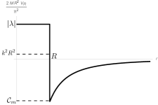
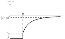
Figure 2: Regularized potential in attractive case. In the region $r<R$ we have: (a) A barrier potential, $\lambda<0$; (b) A well potential, $\lambda>0$.

For the specific case with $E=0$, the requirement for continuity of the wave function and its first derivative leads to the following equality

$$\gamma(R)=\nu_{m}\frac{(1-\varepsilon(L_{m}/R)^{2\nu_{m}})}{(1+\varepsilon(L_{m}/R)^{2\nu_{m}})},$$ (29)

with

$$\gamma(\lambda)\equiv\left\{\begin{array}[]{ll}\sqrt{\lambda}\cot\sqrt{\lambda}-\frac{1}{2},\ \lambda>0,\\ \sqrt{|\lambda|}\coth\sqrt{|\lambda|}-\frac{1}{2},\lambda<0,\end{array}\right.$$ (32)

where $\gamma$ is named as the “running coupling constant”. We shall restrict our analysis to the range $-\infty<\lambda<\pi^{2}$ only, where $\gamma(\lambda)$ is a continuous ($\gamma(0^{\pm})=1/2$) and single-valued function defined on the entire real line, as shown in fig. 3. These requirements assure that the equalities (29) and (32) determine the coupling $\lambda$ as a function of the cutoff $R$.

The explicit knowledge of $\gamma(\lambda)$ and $\lambda(R)$ allows us to directly apply the standard field-theoretical and statistical mechanics renormalization group approach to the case of the AB scattering. As usual, the most important quantity is given by the derivative $d\gamma/d(\ln(R/L_{m}))$, representing the beta function, $\beta(\gamma)$, of the regularized AB model and the following section 4 is devoted to its study. As one can easily verify in the two limits of $L_{m}$ the coupling $\gamma$ becomes an $R$-independent constant. The first one is $L_{m}=0$ ($c_{-}=0$), $\gamma\equiv\gamma_{IR}=\nu_{m}$ and $L_{m}\rightarrow\infty$ ($c_{+}=0$), $\gamma\equiv\gamma_{UV}=-\nu_{m}$ is the other one. These are, respectively, the IR and UV fixed points of the model, where only one solution holds and the conformal symmetry is restored. It is assumed that $\lambda(R)$ remains unchanged under the renormalization procedure, i.e. it is given by Eq. (29) for all the energies.

We next consider the $E>0$ case. As the continuity of the logarithmic derivative $u^{\prime}_{m}(r)/u_{m}(r)$ is required at $r=R$, with $kL\ll 1$, we only need the asymptotic expressions

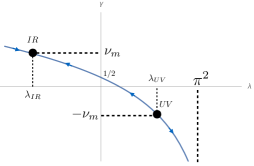
Figure 3: The “running coupling” $\gamma$ as a function of the strength coupling $\lambda$. Within the range $-\infty<\lambda<\sqrt{\pi}$ the parameter $\gamma$ assumes all the values on the line. The arrows indicate the directions of the RG flows, that will be discussed in section 4. The solid dots are the IR and UV fixed points.

$$J_{\nu}(z)\approx\frac{1}{\Gamma(1+\nu)}\left(\frac{z}{2}\right)^{\nu}\,\ \ N_{\nu}(z)\approx-\frac{\Gamma(\nu)}{\pi}\left(\frac{z}{2}\right)^{-\nu},\ z\ll 1,$$

leading to

$$\rho R\cot(\rho R)-1/2\approx\gamma=\nu_{m}\frac{\frac{A_{m}}{\Gamma(1+\nu_{m})}\left(\frac{kR}{2}\right)^{\nu_{m}}+B_{m}\frac{\Gamma(\nu_{m})}{\pi}\left(\frac{kR}{2}\right)^{-\nu_{m}}}{\frac{A_{m}}{\Gamma(1+\nu_{m})}\left(\frac{kR}{2}\right)^{\nu_{m}}-B_{m}\frac{\Gamma(\nu_{m})}{\pi}\left(\frac{kR}{2}\right)^{-\nu_{m}}}.$$

By eliminating $\gamma$ with the help of Eq. (29), one can easily derive the explicit form of the ratio $B_{m}/A_{m}$:

$$\frac{B_{m}}{A_{m}}=\frac{(-\varepsilon)\pi}{\Gamma(\nu_{m})\Gamma(1+\nu_{m})}\left(\frac{kL_{m}}{2}\right)^{2\nu_{m}},\ 0<\nu_{m}<1.$$ (33)

Once the renormalization process has been completed, the ratio of the constants $A_{m}$ and $B_{m}$ have been uniquely fixed as a function of the length scale $L_{m}$ only, i.e. independent of the “cut-off” scale $R$, as expected. Then the renormalized cylindrical wave function for the modes $m=-n$ or $m=-n-1$ takes the form:

$$R^{ren}_{m}(r)=A_{m}J_{\nu_{m}}(kr)+B_{m}N_{\nu_{m}}(kr),\ r>R,$$ (34)

where the constants $A_{m}$ and $B_{m}$ are now related by Eq. (33). In the limit $kr\gg 1$ we get

$$R^{ren}_{m}(r)\approx\sqrt{\frac{2}{\pi kr}}\left[A_{m}\cos\left(kr-\frac{\pi}{4}-\frac{\pi}{2}\nu_{m}\right)+B_{m}\sin\left(kr-\frac{\pi}{4}-\frac{\pi}{2}\nu_{m}\right)\right].$$ (35)

By comparing with the boundary condition (69), required by the elastic scattering, we realize that

$$R^{ren}_{m}(r)\approx\sqrt{\frac{2}{\pi kr}}\sin\left(kr-\frac{\pi}{2}\left(m-\frac{1}{2}\right)+\frac{\pi}{2}\left(m-\nu_{m}\right)+\Sigma_{m}\right),$$

where we have introduced the parameterization $A_{m}=\cos\Sigma_{m}$ and $B_{m}=-\sin\Sigma_{m}$ in terms of the correction $\Sigma_{m}$ to the phase shifts,

$$\tan\Sigma_{m}(k)=\frac{\varepsilon\pi}{\Gamma(\nu_{m})\Gamma(1+\nu_{m})}\left(\frac{kL_{m}}{2}\right)^{2\nu_{m}}.$$ (36)

The above results demonstrate that the renormalization of the Calogero potential (for fixed $m$) generates a one-parameter family of models, i.e. exactly the same conclusion as the one obtained in [8] by the self-adjoint extensions methods. Finally, we find as a consequence of the above equations the explicit form of the new renormalized phase-shifts ($\zeta\neq 0$):

$$\delta^{ren}_{m}=\left\{\begin{array}[]{ll}\frac{\pi}{2}\left(m-\nu_{m}\right)+\Sigma_{m},\ m=-n,\ m=-n-1,\\ \frac{\pi}{2}\left(m-\nu_{m}\right),\textrm{others values of $m$}.\end{array}\right.$$ (39)

Let us remind that if $\zeta=1/2$, $\nu_{n}=\nu_{n-1}=1/2$, and the two scales do coincide, $L_{n}=L_{-n-1}$, then a degeneracy for the phase-shifts corrections $\Sigma_{n}=\Sigma_{n-1}$ arises.

When the magnetic flux is quantized ($\Phi/\Phi_{0}\in\mathbb{N}$), i.e. for $\zeta=0$, the unique mode $m=-n$ needs to be renormalized. In this case the renormalized solutions turn out to be completely different, and all the process has to be reformulated. We start again with the zero energy case:

$$u_{-n}(r)=\left\{\begin{array}[]{ll}\sqrt{r}\left(1+\bar{c}\ln(r/L)\right),\ r>R,\\ \sqrt{R}\left(1+\bar{c}\ln(R/L)\right)\frac{\sin\left(\sqrt{\lambda}r/R\right)}{\sin\sqrt{\lambda}},\ r<R,\end{array}\right.$$ (42)

where $\bar{c}$ is a dimensionless constant and $L$ defines again the length scale. The continuity of $u^{\prime}_{m}(r)/u_{m}(r)$ now implies:

$$\gamma(R)=\frac{\bar{c}}{1+\bar{c}\ln(R/L)},$$ (43)

with the same $\gamma(\lambda)$ as in Eq. (32). We next reconsider the renormalization procedure for $E>0$:

$$u_{-n}(r)=\left\{\begin{array}[]{ll}A_{-n}\sqrt{r}J_{0}(kr)+B_{-n}N_{0}(kr),\ r>R,\\ \left[A_{-n}\sqrt{R}J_{0}(kR)+B_{-n}\sqrt{R}N_{0}(kR)\right]\frac{\sin(\rho r)}{\sin(\rho R)},\ \rho=\frac{1}{R}\sqrt{\lambda+(kR)^{2}}\ r<R.\end{array}\right.$$ (46)

Again, the continuity of $u_{-n}^{\prime}(r)/u_{-n}(r)$, together with the hypothesis $kR\ll 1$, yield

$$\gamma(\lambda)=\frac{\Theta}{1+\Theta\ln(kR)},\ \ \Theta\equiv\frac{2}{\pi}\left(\frac{A_{-n}}{B_{-n}}+\frac{2C_{E}}{\pi}\right)^{-1},$$ (47)

where $C_{E}\approx 0.5772$ is the Euler’s constant and the following asymptotic forms

$$J_{0}(z)\approx 1+\mathcal{O}(z^{2}),\ \ \ N_{0}(z)\approx\frac{2}{\pi}\left(\ln(z/2)+C_{E}\right)+\mathcal{O}(\ln(z/2)z^{2}),$$

have been used. Finally, by eliminating $\gamma(\lambda)$ from the above expression

$$\frac{A_{-n}}{B_{-n}}=\frac{2}{\pi}\left(\frac{1}{\bar{c}}-C_{E}-\ln(kL)\right)=-\frac{2}{\pi}\ln(k\bar{L}),\ \bar{L}=e^{-\frac{1}{\bar{c}}+C_{E}}L,$$ (48)

the real physical prediction (without any cutoff $R$-dependence) is obtained. The corresponding renormalized cylindrical wave function now takes the asymptotic form

$$R^{ren}_{-n}(r)\approx\sqrt{\frac{2}{\pi kr}}\left(A_{-n}\cos(kr-\pi/4)+B_{-n}\sin(kr-\pi/4)\right),\ kr\gg 1.$$ (49)

With an appropriate definition

$$A_{-n}=\cos\bar{\Sigma},\ \ B_{-n}=-\sin\bar{\Sigma},$$ (50)

we have again a one-parametric family of consistent models. Observe that the Eq. (69) is obtained once more, but with the new form of the phase-shifts

$$\delta^{ren}_{-n}=-\frac{n\pi}{2}+\bar{\Sigma}(k),\ \ \cot(\bar{\Sigma}(k))=\frac{2}{\pi}\ln(k\bar{L}).$$ (51)

The calculations of the renormalized phase-shifts for all the cases of interest (i.e. for all allowed values of $\zeta$), that by construction are cut-off independent, provides a firm base for the construction of the physically relevant and observable quantities, which in the context of the AB problem are in fact reduced to the knowledge of the corrections to the original AB elastic scattering cross-section.

3.2 Renormalized scattering amplitudes

Once we have the renormalized phase-shifts, all the scattering data is at our hands. What remains is to derive the renormalized scattering amplitudes. Let us start with the case $\zeta\neq 0$:

$$f_{k}^{ren}= \frac{e^{-in\varphi}}{i\sqrt{2\pi k}}\sum_{m=-\infty}^{\infty}\left(e^{2i\delta_{m}^{ren}}-1\right)e^{im\varphi},$$ (52)

$$= f_{k}+(-1)^{n}e^{-in\varphi}\sqrt{\frac{2}{\pi k}}\left[e^{i\left(\Sigma_{-n}-\pi\zeta\right)}\sin\Sigma_{-n}+e^{i\left(\Sigma_{-n-1}+\pi\zeta-\varphi\right)}\sin\Sigma_{-n-1}\right],$$

$$= \frac{(-1)^{n}e^{-i(n+1/2)\varphi}}{\sqrt{2\pi k}}\Bigg{\{}\frac{\sin(\pi\zeta)}{\sin(\varphi/2)}+\cos\left(\frac{\varphi}{2}-\pi\zeta+2\Sigma_{-n}\right)+\cos\left(\frac{\varphi}{2}-\pi\zeta-2\Sigma_{-n-1}\right)$$ (53)

$$-2\cos\left(\frac{\varphi}{2}-\pi\zeta\right)+i\left[\sin\left(\frac{\varphi}{2}-\pi\zeta+2\Sigma_{-n}\right)-\sin\left(\frac{\varphi}{2}-\pi\zeta-2\Sigma_{-n-1}\right)\right]\Bigg{\}}$$

with $f_{k}$ given by Eq. (17). The new cross-section $\sigma^{ren}_{k}=|f_{k}^{ren}|^{2}$ may be obtained by a direct calculation. Here we will present a simple version of it, valid at the low energy limit, where $\Sigma_{-n}(k),\Sigma_{-n-1}(k)\ll 1$. For $\varphi\neq 0$ we have

$$\sigma_{k}^{(ren)}\approx\frac{1}{2\pi k}\frac{\sin^{2}\pi\zeta}{\sin^{2}(\varphi/2)}+\frac{2}{\pi}\frac{\sin\pi\zeta\sin(\varphi/2-\pi\zeta)}{\sin(\varphi/2)}\left(\frac{\Sigma_{-n-1}(k)-\Sigma_{-n}(k)}{k}\right).$$ (54)

The two terms of the first correction turn out to have a simple power-law behavior $\Sigma_{-n}(k)/k\sim k^{2\zeta-1}$ and $\Sigma_{-n-1}(k)/k\sim k^{1-2\zeta}$. Therefore at low enough energies, and for $\zeta\neq 1/2$, one contribution is always dominating over the other one, while for $\zeta=1/2$ the above first correction is in fact energy independent.

For the configuration with $\zeta=1/2$ and $L_{-n}=L_{-n-1}\equiv L$, i.e. for $\Sigma_{-n}(k)=\Sigma_{-n-1}(k)\equiv\Sigma^{1/2}(k)=\arctan(kL)$, the exact result takes a rather simple and compact form ($\varphi\neq 0$):

$$\sigma^{ren}_{k}(\varphi)=\frac{1}{2\pi k\,\sin^{2}(\varphi/2)}\left[\left(1-4\sin^{2}\left(\Sigma^{1/2}(k)\right)\sin^{2}\left(\frac{\varphi}{2}\right)\right)^{2}+4\sin^{2}\left(2\Sigma^{1/2}(k)\right)\sin^{4}\left(\frac{\varphi}{2}\right)\right].$$

The case $\zeta=0$ ($\Phi/\Phi_{0}\in\mathbb{N}$) is very special. The usual AB cross-section vanishes for $\varphi\neq 0$, and all the contribution comes from the renormalization. After a simple calculation we get

$$\bar{\sigma}_{k}^{ren}=\frac{2}{\pi k}\sin^{2}\bar{\Sigma}=\frac{\pi}{2k}\frac{1}{\pi^{2}/4+\ln^{2}(k\bar{L})}.$$ (55)

This result coincides with the general cross-section for a slow particle ($k\bar{L}\ll 1$) interacting with a short-range potential, or even with the scattering in an impenetrable cylinder of radius $r_{c}=2\bar{L}/C_{E}$, see for example pages $551$-$552$ of ref. [35]. The above formula (55) can also be seen as the cross-section of the renormalized Dirac delta function potential, [36, 37]. Independently of the interpretations, our formula (55) describes a non-trivial isotropic AB scattering which indicates a local short-range interaction.

3.3 Physical interpretation for the new scales as bound states

By construction, our regularization procedure introduces a short-range well potential relevant for the modes within the interval $0\leq\nu_{m}<1$. This fact opens the possibility for existence of bound states with certain angular momenta $m=-n$ e $m=-n-1$ that might survive the $R\rightarrow 0$ limit. In order to analyze this option, let us further assume that $E<0$, and $k_{b}^{(m)}=\sqrt{-2ME/\hbar^{2}}$. The corresponding bound states wave function needs to be square-integrable at infinity. Thus for the regularized solution for $\zeta\neq 0,$ we obtain

$$u_{m}(r)=\left\{\begin{array}[]{ll}D_{m}\sqrt{r}\,K_{\nu_{m}}\left(k_{b}^{(m)}r\right),\ r>R,\\ D_{m}\sqrt{R}\,K_{\nu_{m}}\left(k_{b}^{(m)}R\right)\frac{\sin\left(\rho r\right)}{\sin(\rho R)},\ \rho=\frac{1}{R}\sqrt{\lambda-(k_{b}^{(m)}R)^{2}},\ r<R,\end{array}\right.$$ (57)

where $K_{\nu_{m}}(z)$ is the modified Bessel function of the second kind [17]. Once again, by hypothesis $R$ is a small scale such that $k_{b}^{(m)}R\ll 1$, so around $r=R$, $\sin(\rho r)\approx\sin\sqrt{\lambda}$ and we only need the corresponding asymptotic expressions

$$K_{\nu}(z)\approx\frac{1}{\Gamma(1-\nu)}\left(\frac{z}{2}\right)^{-\nu}-\frac{1}{\Gamma(1+\nu)}\left(\frac{z}{2}\right)^{\nu},\ z\ll 1.$$

Then the continuity of $u^{\prime}_{m}(r)/u_{m}(r)$ at $r=R$ can be read as

$$\sqrt{\lambda}\cot\sqrt{\lambda}-\frac{1}{2}\equiv\gamma=-\nu_{m}\,\frac{1+\frac{\Gamma(1+\nu_{m})}{\Gamma(1-\nu_{m})}\left(\frac{2}{k_{b}^{(m)}R}\right)^{2\nu_{m}}}{1+\frac{\Gamma(1+\nu_{m})}{\Gamma(1-\nu_{m})}\left(\frac{2}{k_{b}^{(m)}R}\right)^{2\nu_{m}}}.$$ (58)

Now by comparing with equation (29) and solving for $k_{b}$ we find

$$k_{b}^{(m)}=\left(\frac{1}{-\varepsilon}\frac{\Gamma(1+\nu_{m})}{\Gamma(1-\nu_{m})}\right)^{\frac{1}{2\nu_{m}}}\frac{2}{L_{m}}.$$ (59)

That is, in the case $\varepsilon=1$ there are no bound states at all, while for $\varepsilon=-1$ each one of the modes $m=-n$ and $m=-n-1$ corresponds to a bound state when $k_{b}^{(m)}R\ll 1$. In the particular case when the two scales coincide, i.e. for $L_{-n}=L_{-n-1}\equiv L$, the ratio

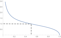
Figure 4: Equation (60).

$$\frac{k_{b}^{(-n-1)}}{k_{b}^{(-n)}}=\left(\frac{\Gamma(1+\zeta)}{\Gamma(1-\zeta)}\right)^{\frac{1}{2\zeta}}\left(\frac{\Gamma(2-\zeta)}{\Gamma(\zeta)}\right)^{-\frac{1}{2(1-\zeta)}}$$ (60)

is completely fixed. As one can see from the curve $k_{b}^{(m)}(\zeta)$ shown on figure 4, in the range $0<\zeta<1/2$ we have $k_{b}^{(-n-1)}>k_{b}^{(-n)}$, while for $1/2<\zeta<1$ the inverse relation $k_{b}^{(-n-1)}<k_{b}^{(-n)}$ holds; the degeneracy $k_{b}^{(-n-1)}=k_{b}^{(-n)}$ occurs for magnetic fluxes with $\zeta=1/2$. In conclusion, for $\varepsilon=-1$ the new scales correspond to the energies of certain bound states and we can eliminate them (both $L_{-n}$ and $L_{-n-1}$ as well), in favor of $k_{b}^{(-n)}$ and $k_{b}^{(-n-1)}$ in the cross-section. Notice that in the derivation of the bound states energies we have assumed that $k_{b}^{(m)}R\ll 1$, which results in $k_{b}^{(m)}\sim 1/L_{m}$ and as a consequence we have $R<L_{m}$, so that such bound states do exist even in the limit $R\rightarrow 0$.

For quantized fluxes $\Phi/\Phi_{0}\in\mathbb{N}$ (i.e. for $\zeta=0$) the procedure is quite similar. The main differences comes from the behavior of $K_{0}(z)$ around the origin

$$K_{0}(z)\approx-C_{E}-\ln(z/2),\ z\ll 1,$$

and the fact that now $\gamma$ is given by (43). Following the steps we have already made in the previous more general case, we find for the bound state energy

$$k_{b}^{(-n)}=\frac{2}{\bar{L}}.$$ (61)

The cross-section (55) in this particular case has quite a clear meaning. Like the two-dimensional scattering in Dirac delta function potential, we are dealing with a non-relativistic exemple of the dimensional transmutation due to the existence of a bound state responsible for the anomalous behavior of the cross-section [36, 37],

$$\bar{\sigma}_{k}^{ren}=\frac{\pi}{2k}\frac{1}{\pi^{2}/4+\ln^{2}\left(2k/k_{b}^{(-n)}\right)}\sim\frac{1}{k\ln^{2}\left(2k/k_{b}^{(-n)}\right)},\ k/k_{b}^{(-n)}\gg 1.$$ (62)

The above discussion about the existence of bound states in the AB problem might sound rather meaningless, since the Calogero potential, $2MV(r)/\hbar^{2}=\mathcal{C}_{m}/r^{2}$, is repulsive in the range $1/2\leq\zeta<1$ ($0\leq\mathcal{C}_{m}<3/4$). Thus the bound states can only be associated to the short-range well potentials introduced by the regularization procedure, see figures 1 and 2. But for the specific AB solenoid this makes perfect sense, since in the interior of a transversal magnetic field the motion of a charged particle is bounded, thus creating the Landau energy levels. So, in the $\varepsilon=-1$ case, up to two Landau levels — for which the particle is “trapped” within the solenoid — will survive even in the null radius limit. Indeed, the probability to find the particle outside the solenoid (in the classically forbidden region) is exponentially suppressed by the behavior $|\sqrt{r}K_{\nu_{m}}(k_{b}^{(m)}r)|^{2}\sim e^{-2k_{b}^{(m)}r}$ for $k_{b}^{(m)}r\gg 1$. Notice that the two allowed bound states have definite values of the angular momentum in the direction of the field, $m=-n$ and $m=-n-1$, reflecting the fact that the trapped particle rotates clockwise, due to the negative sign choice, $-|e|$, of its electric charge.

4 AB Beta function and RG flows

The rich variety of options and interesting physical phenomena behind the renormalization procedure needed for the correct description of the AB scattering (including the ones related to the presence or not of bound states) represent a subject already known in the Calogero potential literature, not only for the strong coupling region $\mathcal{C}_{m}<-1/4$, which is not relevant for the AB scattering problem, but also in the “medium-weak”-range $-1/4\leq\mathcal{C}_{m}<3/4$, see [34]. On the other hand, it is not usual (although there are some exceptions [38, 39]) to explore how all these options can be understood in a clear and elegant way within the framework of the renormalization group (RG) methods and, related to it, to the concepts of critical points, phase transitions and RG flows. This section is dedicated to this subject.

The “running coupling” $\gamma$ for each $m$-mode is given by (29) (for $\zeta\neq 0$ and $m=-n,-n-1$) or by (43) (for $\zeta=0$ and $m=-n$). Defining the adimensional scale $l=\ln(R/L_{m})$ and taking the derivative of (29) one can easily obtain the exact beta function for the considered AB scattering problem

$$\frac{d\gamma}{dl}\equiv\beta_{\gamma}=-\left(\gamma+\nu_{m}\right)\left(\gamma-\nu_{m}\right),$$ (63)

which turns out to have two fixed (critical) points $\beta_{\gamma}(\gamma^{*})=0$. The IR stable one corresponds to $\gamma_{IR}=\nu_{m}$ ($c_{-}=0$ in (22)) and a conformal dimension $\Delta_{IR}=-2\nu_{m}$, while the unstable UV fixed point is characterized by $\gamma_{UV}=-\nu_{m}$ ($c_{+}=0$ in (22)) and a conformal dimension $\Delta_{UV}=2\nu_{m}$. The beta function behavior, together with the RG flow relating these two critical points, is shown on figure 5. By construction, Eq. (29) is the general solution of (63) with $\varepsilon L_{m}^{2\nu_{m}}$ as an integration constant. Let us rewrite the equation in terms of the new parameter $l$

$$\gamma(l)=\nu_{m}\frac{1-\varepsilon e^{2\nu_{m}l}}{1+\varepsilon e^{2\nu_{m}l}}.$$ (64)

Now we will analyze the role of the $\varepsilon$ sign.

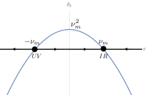
Figure 5: Beta function (63). The arrows indicate the RG flow and the dots are the fixed points.

• If $\varepsilon=1$, then $l$ runs over all the scales, $-\infty<l<\infty$, and $\gamma_{UV}=-\nu_{m}<\gamma<\nu_{m}=\gamma_{IR}$, as shown by the blue curve in figure 6. This RG flow doesn’t have a characteristic length scale (in the RG language it is a massless flow) going from the UV fixed point to the IR one. As one can see from figure 3 the original coupling $\lambda\in(\lambda_{IR},\lambda_{UV})$, with $\lambda_{IR}<0$ and $\lambda_{UV}>0$ when $\nu_{m}>1/2$. Therefore a bound state is impossible as $\lambda$ can change sign in the vicinities of the IR point and the well potential turns into a repulsive barrier potential. The absence of natural scales prevents the existence of bound states.

  Note that our specific choice $-\infty<\lambda<\pi^{2}$ ($-\infty<\gamma<\infty$) of the $\lambda$-interval is crucial for the compatibility among the RG flow description and the regularized potential — this fact was missed in ref. [9, 34], where $\lambda>0$ is assumed. As the cutoff is unbounded, for large $R$ a bound state would be unavoidable if $\lambda$ was always positive, thus leading to an inconsistency. Already in the vicinities of the UV energy regime the condition $kR\ll 1$ still holds, and in the regularized region $r<R$ we have a deep well potential ($\sim\lambda/R^{2}$), which does not support a bound state and diverges in the $R\rightarrow 0$ and $\lambda\rightarrow\lambda_{UV}^{-}$ limits.

• The conclusions are absolutely different for the $\varepsilon=-1$ case. Now the scale $R$ has $L$ as its maximum or minimum value (in the RG language this corresponds to a massive flow) since $\gamma(l)$ diverges when $l\rightarrow 0$. For the “initial scale condition” $l_{0}<0$ ($R_{0}<L_{m}$) we have $-\infty<\gamma(l)<-\nu_{m}$ with $-\infty<l<0$, see the red line on the third quadrant of figure 6, so that $L_{m}$ is the maximum value permitted for the cut-off $R$. Therefore, along the entire RG flow $\gamma<1/2$ ($\lambda>0$) the “short-range” potential is represented by the potential well. In this case, the $R$-independent bound state given by Eq. (59) is present even if the Calogero potential is repulsive, because (59) implies that $k_{b}^{(m)}\sim 1/L_{m}$ and thus the existence condition for such a state, $k_{b}^{(m)}R\sim R/L_{m}\ll 1$, is fulfilled in the $R\rightarrow 0$, $\lambda\rightarrow\lambda_{UV}^{+}$ limits. Now the meaning of $\lambda_{UV}$ becomes evident: it is the critical coupling value that regulates the existence ($\lambda>\lambda_{UV}$) or not ($\lambda<\lambda_{UV}$) of the bound state in the $R\rightarrow 0$ limit.

  

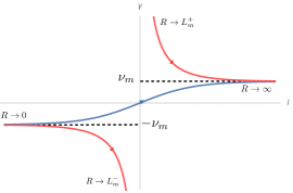
  Figure 6: Curves for Eq. (64); the blue one is for $\varepsilon=1$ and the red ones are for the $\varepsilon=-1$ case.

  Another possibility for $\varepsilon=-1$ occurs when the RG “initial condition” is given by $\gamma(l_{0})>\nu_{m}$. The running coupling range is now $\nu_{m}<\gamma<\infty$ and $l>0$, see red curve on the first quadrant of figure 6. Since $\gamma$ can be arbitrarily large ($R\rightarrow L^{+}$) and consequently $|\lambda|\gg 1$, with $\lambda<0$, so that in this limit the potential in the region $r<R$ is a repulsive barrier. Hence in this case we still have a characteristic length, but not a bound state. In fact, the condition $k_{b}^{(m)}R\sim R/L_{m}\ll 1$ cannot be satisfied. Such a flow is not related with the Calogero potential renormalization, since the limit $R\rightarrow 0$ is now not available. In fact, it represents the “inverse situation” — a physical barrier potential regularized by an IR Calogero cutoff ($R>L_{m}$), and at the end of the renormalization the limit $R\rightarrow\infty$ has to be taken. Thus it will be excluded from our analysis.

When the magnetic flux is exactly $\Phi=N\Phi_{0}$, $N\in\mathbb{N}^{*}$, the UV and IR fixed points of the mode $m=-n$ ($\nu_{-n}=0$) “collide” in one new marginal point, $\gamma_{UV}=\gamma_{IR}=0$ and the maximum of the parabola in fig. 5 touches the horizontal axis. The beta function for this case is

$$\beta_{\gamma}=-\gamma^{2}.$$ (65)

The passage from (63) to (65) is known as a BKT-like phase transition [14, 15, 16]. The integration of (65) leads to (43) with $\bar{c}$ being the integration constant. In this limit the massless flow between the two fixed points disappears from the figures 5 and 6. Now only the $\gamma=0$ fixed point has no intrinsic scale and the conformal symmetry takes place for the solution with $\bar{c}=0$. To its left ($\bar{c}<0$) we have an unstable massive flow with a maximal scale $L_{-n}$, and to its right ($\bar{c}>0$) the massive stable flow with a minimal scale $L_{-n}$. Like in the previous case, the bound state is associated to the unstable flow, because the limit $R\rightarrow 0$ can be taken. The stable massive case must be excluded once again, since the region $r<R$ cannot be made arbitrary small. The absence of parameters in the beta function (65) show us that all the magnetic fluxes $N\Phi_{0}$ belong to the same universality class, reflecting the periodic behavior of the physical observables in the AB Scattering. It also suggests that the $\bar{L}$-scale (defining the bound state energy (61)) is independent of $N$ as well.

Our last comment is about the attractive region of the Calogero potential that is not realized in the AB Scattering, i.e. the case of “strong-attraction”-coupling $\mathcal{C}_{m}<-1/4$. We can adapt our results for this case as well with a formal change of the variables: $\nu_{m}\rightarrow ig$ ($g\in\mathbb{R}$). Now the beta function takes the form

$$\beta_{g}(\gamma)=-\gamma^{2}-g^{2},$$ (66)

without any real zeros; that is, the maximum of the parabola on fig. 5 is now below the horizontal axis. By integrating this beta function one can find the running-coupling scale dependence $\gamma(l)=-g\tan(gl-\phi_{0})$. Its $2\pi/g$-periodic behavior, which corresponds to the periodic region $\lambda>\pi^{2}$ in the definition of $\gamma(\lambda)=\sqrt{\lambda}\cot\sqrt{\lambda}$, generates an infinite chain of scales, leading to an infinite number of bound states accumulated in the low energies region. This phenomenon is known as the Efimov effect commented earlier in section 3.

5 Conclusions

In this paper we have revisited in details the elastic scattering of a non-relativistic charged particle without spin in an ideal magnetic field $\vec{B}=B_{0}\,\delta(x)\delta(y)\hat{z}$ — the AB scattering problem. Since our analysis is based on the phase-shifts method, we have rewritten the incident wave function $e^{ikx}e^{i\alpha(\varphi-\pi)}$ as $e^{ikx}+2ie^{ikx}e^{i\alpha(\varphi-\pi)/2}\sin[\alpha(\varphi-\pi)/2]$ and the second term was “hidden” in the outgoing cylindrical wave function. Our choice of standard scattering boundary conditions allows us to derive the AB scattering amplitude in an easy and direct way, including an extra $\delta$-term, important for the unitarity of the S-Matrix.

We have implemented, in our study of the correct self-adjoint extension of the cylindrical AB Hamiltonian, the renormalization methods specific for the one-dimensional Calogero model, by taking into account the advantages of the established AB scattering/Calogero correspondence. We have demonstrated that, depending on the values of the magnetic flux, one or two of the phase-shifts modes have to be renormalized. As a consequence, the AB cross-section receives certain renormalization corrections, parametrized by at most two new scales associated to the bound states energies. We expect that our approach, combining the phase-shift method and the renormalization group, could be successfully adapted to the correct description of the AB scattering of non-relativistic spin-$1/2$ particles, by considering an appropriate self-adjoint extension of the Pauli equation, as well as to the relativistic RG corrections to the high-energy electron scattering cross-section in terms of the renormalized solutions of the Dirac equation in an external magnetic field created by an infinitely thin solenoid.

Since the emergence of new physical scales appears to be one of the essencial elements of our renormalization of the AB scattering amplitudes, we find worthwhile to comment once more on their physical meaning. One can adopt a rather conservative point of view, observing that the finite solenoid problem has also two natural scales: the solenoid radius $r_{c}$ and the magnetic field strength $r_{B}=\left(B|e|/\hbar\right)^{-1/2}$. In the “infinitely thin solenoid” limit, both scales go to zero with a fixed ratio $\left(r_{c}/r_{B}\right)^{2}=2\Phi/\Phi_{0}$. Therefore the physical results are functions of this ratio only, and the conformal symmetry should be preserved. One can further try to relate the renormalization scales with these natural scales, e.g. $r_{c}\sim L_{-n}$ and $r_{B}\sim L_{-n-1}$, so the renormalized cross-section we have derived can be regardaded as describing a more realistic scattering problem involving a finite solenoid and a finite magnetic field. Apparently this does not seems to be the case, since after renormalization the $R$ cutoff becomes arbitrarily small, making clear that we are dealing with an infinitely thin solenoid, and also because of the fact that our cross-section does not agree with the results obtained in the WKB approximation for solenoids of finite radius [22].

An argument in favor of the quantum origin of the new energy scales comes from the fact that all the different scattering amplitude corrections predicted by the renormalization process can be explained by the RG flow of the $\gamma$-running coupling. We have demonstrated that a few different RG flows (massive and massless) can be realized. The case $\varepsilon=1$ represents a massless RG flow connecting the UV and IR regimes without any characteristic length scale. Instead, for the $\varepsilon=-1$ case a massive RG flow occurs and now the scale $L_{m}$ appears as the maximum or the minimum value of the $R$ cutoff. Since our interest is in short-range values of the cutoff, it is assumed that $L_{m}$ is the greatest length scale corresponding to the flow that leaves the UV fixed point and goes to minus infinity ($-\infty<\gamma<-\nu_{m}$). Along this flow, in the region $r<R$, there is a potential well that supports one bound state with energy $\sim 1/L_{m}^{2}$. As we have shown, one or two of the Landau levels can survive and the cross-section appears to be a function of the corresponding bound states energies. This phenomenon provides an example of dimensional transmutation, where the conformal symmetry is spontaneously broken during the renormalization process that creates certain quantum scale anomaly. Their exact values can be determined by experimental observation only. It is important to emphasize that, in all the cases, the IR fixed point is a part of the coupling-space. So we can have two, one or zero new scales; in the last case the conformal symmetry is still preserved and the AB cross-section remains unchanged coinciding with the original one (18).

The most relevant aspect arising from the renormalization of the AB Scattering problem is the universal phase-shift deviation $2\delta_{-N}^{ren}+N\pi=2\bar{\Sigma}(k)\neq 0$ for the quantized magnetic flux case, $\Phi=N\Phi_{0}$ (e.g. when the cylinder is a superconductor), leading to a non null, isotropic and energy dependent cross-section, and its relation with a BKT-like phase transition of infinite order. This is an explicit realization of the phase transition in the Calogero potential beyond the Efimov effect — another recent case was observed in a graphene plane at zero temperature [40].

Acknowledgments

I wish to thank E. S. Costa, G. Luchini and G. Sotkov for the productive discussions and G. Sotkov for the great help in the elaboration process of this manuscript.

Appendix A Phase-shifts method for short-range two-dimensional elastic scattering

In this appendix we present a brief review of the quantum elastic scattering in a plane to support the analysis made in the main text. The wave function that describes a particle with energy $E$ launched from $x\rightarrow-\infty$ with momentum $\vec{p}_{in}=\hbar k\,\hat{x}=\sqrt{2ME}\,\hat{x}$ and scattered by a short range external potential obeys the boundary condition

$$\psi(r,\varphi)\approx e^{ikx}+f_{k}(\varphi)\frac{e^{ikr}}{\sqrt{-ir}},\ x=r\cos\varphi,\ kr\gg 1.$$ (67)

The angular function $f_{k}(\varphi)$ is the scattering amplitude and the cross-section is defined by $\sigma_{k}=|f_{k}(\varphi)|^{2}$. This asymptotic behavior is fulfilled by the following ansatz, see pages $507-508$ of [35]

$$\psi_{k}(r,\varphi)=\sum_{m=-\infty}^{\infty}i^{m}e^{i\delta_{m}}Q_{m}^{(k)}(r;\delta_{m})e^{im\varphi},$$ (68)

where the function $Q_{m}^{(k)}(r;\delta_{m})$ is the solution of the cylindrical equation such that

$$Q_{m}^{(k)}(r;\delta_{m})\approx\sqrt{\frac{2}{kr}}\sin\left(kr-\frac{\pi}{2}\left(m-\frac{1}{2}\right)+\delta_{m}\right),\ kr\gg 1.$$ (69)

The quantities $\delta_{m}$, $m\in\mathbb{Z}$, are the phase-shifts which completely describe the scattering process. Substituting the asymptotic expression (69) in (68) and after some algebraic manipulations making use of the identity, see page $114$ of [35]

$$e^{ikx}=\sum_{m=-\infty}^{\infty}i^{m}J_{m}(kr)e^{im\varphi},$$ (70)

the result (67) is easily found with the scattering amplitude being given by

$$f_{k}(\varphi)=\frac{1}{i\sqrt{2\pi k}}\sum_{m=-\infty}^{\infty}\left(e^{2i\delta_{m}}-1\right)e^{im\varphi}.$$ (71)

So the elastic scattering problem can be summarized in the search of the phases $\delta_{m}$ ($m\in\mathbb{Z}$) defined by equation (69), together with the summation (71). Being not necessary the direct use of the total wave function (68).

References

References

- [1] M. Peshkin, A. Tonomura, The Aharonov-Bohm Effect, Lecture Notes in Physics, Springer; Softcover reprint of the original 1st ed. 1989 edition, 2013.
- [2] A. Tonomura, The ab effect and its expanding applications, Journal of Physics A: Mathematical and Theoretical 43 (35).
- [3] Y. Aharonov, D. Bohm, Significance of electromagnetic potentials in the quantum theory, Phys. Rev. 115 (3).
- [4] R. G. Chambers, Shift of an electron interference pattern by enclosed magnetic flux, Phys. Rev. Lett. 5 (3).
- [5] T. T. Wu, C. N. Yang, Concept of nonintegrable phase factors and global formulation of gauge fields, Phys. Rev. D 12 (12) (1975) 3845–3857.
- [6] E. Merzbacher, Single valuedness of wave functions, American Journal of Physics 30 (237).
- [7] S. Ruijsenaars, The aharonov-bohm effect and scattering theory, Annals of Physics 146 (1) (1983) 1 – 34.
- [8] D. Gitman, I. Tyutin, B. Voronov, Self-adjoint Extensions in Quantum Mechanics: General Theory and Applications to Schrödinger and Dirac Equations with Singular Potentials, 1st Edition, Birkhäuser, 2012.
- [9] S. R. Beane, P. F. Bedaque, L. Childress, A. Kryjevski, J. McGuire, U. V. Kolck, Singular potentials and limit cycles, Phys. Rev. A 64 (2001) 042103.
- [10] D. Gitman, I. Tyutin, B. Voronov, Self-adjoint extensions and spectral analysis in calogero problem, Journal of Physics A: Mathematical and Theoretical 43 (14) (2010) 145205.
- [11] F. Calogero, Solution of a three‐body problem in one dimension, Journal of Mathematical Physics 10.
- [12] F. Calogero, Solution of the one‐dimensional n‐body problems with quadratic and/or inversely quadratic pair potentials, Journal of Mathematical Physics 12.
- [13] S. Coleman, E. Weinberg, Radiative corrections as the origin of spontaneous symmetry breaking, Phys. Rev. D 7 (1973) 1888–1910.
- [14] V. Berezinskii, Destruction of long-range order in one-dimensional and two-dimensional systems having a continuous symmetry group i. classical systems, Sov. Phys. JETP 32 (3) (1970) 493.
- [15] V. Berezinskii, Destruction of long-range order in one-dimensional and two-dimensional systems possessing a continuous symmetry group. ii. quantum systems, Sov. Phys. JETP 34 (3) (1971) 610.
- [16] J. M. Kosterlitz, D. J. Thouless, Ordering, metastability and phase transitions in two-dimensional systems, Journal of Physics C: Solid State Physics 6 (7) (1973) 1181.
- [17] A. Erdelyi, H. Bateman, Higher Transcendental Functions Bateman Manuscript Project Volume I One 1, 1st Edition, McGraw-Hill Book Company, Inc., 1953.
- [18] M. V. Berry, Aharonov-bohm wavefunction obtained by applying dirac’s magnetic phase factor, Eur. J. Phys. 1 (1980) 220–144.
- [19] S. Sakoda, M. Omote, Aharonov-mohm scattering: The role of the incident wave, Journal of Mathematical Physics 38 (2).
- [20] Y. Sitenko, N. Vlasii, The aharonov–bohm effect in scattering theory, Annals of Physics 339 (2013) 542 – 559.
- [21] Y. A. Sitenko, The aharonov-bohm effect in scattering of nonrelativistic electrons by a penetrable magnetic vortex, Quantum Studies: Mathematics and Foundations 1 (3 - 4) (2014) 213 – 222.
- [22] O. Yilmaz, Scattering of a charged particle from a hard cylindrical solenoid: Aharonov-bohm effect, Chin.J.Phys. 52.
- [23] C. R. Hagen, Aharonov-bohm scattering amplitude, Physical Review D 41 (6).
- [24] J. Dereziński, S. Richard, On schrödinger operators with inverse square potentials, Ann. Henri Poincaré 18 (3) (2017) 869 – 928.
- [25] P. Naidon, S. Endo, Efimov physics: a review, Reports on Progress in Physics 80 (5) (2017) 056001.
- [26] V. N. Efimov, Weakly-bound states of three resonantly-interacting particles, Soviet Journal of Nuclear Physics 12 (5) (1970) 589–591.
- [27] V. Efimov, Energy levels arising from resonant two-body forces in a three-body system, Physics Letters B 33 (8) (1970) 563 – 564.
- [28] H. E. Camblong, L. N. Epele, H. Fanchiotti, C. A. G. Canal, Renormalization of the inverse square potential, Physical Review Letters 85 (8).
- [29] H. E. Camblong, L. N. Epele, H. Fanchiotti, C. A. G. Canal, Dimensional transmutation and dimensional regularization in quantum mechanics: I. general theory, Annals of Physics 287 (1) (2001) 14 – 56.
- [30] S. A. Coon, Anomalies in quantum mechanics: the 1/r2 potential, American Journal of Physics 70 (513).
- [31] E. Braaten, D. Phillips, The renormalization group limit cycle for the 1/r2 potential, Physical Review A 70 (5) (2004) 052111.
- [32] H. E. Camblong, L. N. Epele, H. Fanchiotti, C. A. G. Canal, C. R. Ordóñez, On the inequivalence of renormalization and self-adjoint extensions for quantum singular interactions, Physics Letters A 364 (6) (2007) 458 – 464.
- [33] C. Burgess, P. Hayman, M. Williams, L. Zalavári, Point-particle effective field theory i: classical renormalization and the inverse-square potential, Journal of High Energy Physics 2017 (4) (2017) 106.
- [34] D. Bouaziz, M. Bawin, Singular inverse-square potential: Renormalization and self-adjoint extensions for medium to weak coupling, Phys. Rev. A 89 (2) (2014) 022113.
- [35] L. D. Landau, L. M. Lifshitz, Quantum Mechanics, Course of Theoretical Physics Vol. 3, 3rd ed. (Elsevier Butterworth-Heinemann), 1977.
- [36] R. Jackiw, Diverse Topics in Theoretical and Mathematical Physics, World Scientific Publishing Company, 1995.
- [37] K. Huang, Quarks, Leptons and Gauge Fields, 2nd Edition, World Scientific Publishing Company, 1992.
- [38] D. B. Kaplan, J.-W. Lee, D. T. Son, M. A. Stephanov, Conformality lost, Phys. Rev. D 80 (12) (2009) 125005.
- [39] K. M. Bulycheva, A. S. Gorsky, Limit cycles in renormalization group dynamics, Physics-Uspekhi 57 (2) (2014) 171.
- [40] O. Ovdat, J. Mao, Y. Jiang, E. Y. Andrei, E. Akkermans, Observing a scale anomaly and a universal quantum phase transition in graphene, Nature Communications 8 (1) (2017) 507.