ReaS: Combining Numerical Optimization with SAT Solving

Abstract.

In this paper, we present ReaS, a technique that combines numerical optimization with SAT solving to synthesize unknowns in a program that involves discrete and floating-point computation. ReaS makes the program end-to-end differentiable by smoothing any Boolean expression that introduces discontinuity such as conditionals and relaxing the Boolean unknowns so that numerical optimization can be performed. On top of this, ReaS uses a SAT solver to help the numerical search overcome local solutions by incrementally fixing values to the Boolean expressions. We evaluated the approach on 5 case studies involving hybrid systems and show that ReaS can synthesize programs that could not be solved by previous SMT approaches.

1. Introduction

Gradient-based numerical techniques are becoming a popular mechanism for solving program synthesis problems. Neural networks have shown that by doing automatic differentiation over complex computational structures (deep networks), they can solve many complex, real world problems (Hinton et al., 2012; Krizhevsky et al., 2012; Silver et al., 2016). There is also a growing body of work on using neural networks to learn programs with discrete control structure from examples, such as neural Turing machines (Graves et al., 2014) and others that follow similar ideas (Reed and De Freitas, 2015; Kurach et al., 2015; Neelakantan et al., 2015; Kaiser and Sutskever, 2015). For many problems with discrete structure, however, recent work (Gaunt et al., 2016) has shown that neural networks are not as effective as state-of-the-art program synthesis tools like Sketch (Solar-Lezama et al., 2006; Solar-Lezama, 2008) that is based on SAT and SMT solving.

This paper shows that a combination of SAT and gradient-based numerical optimization can be effective in solving synthesis problems that involve both discrete and floating-point computation. The combination of numerical techniques and SAT is not itself new; SMT solvers such as Z3 (De Moura and Bjørner, 2008), dReal (Gao et al., 2013a) and the more recent work on satisfiability modulo convex optimization (SMC)  (Shoukry et al., 2017) have also explored problems involving the combination of discrete structure and continuous functions using the DPLL(T) framework (Ganzinger et al., 2004). However, we show that the approach followed by SMT solvers, while effective for many applications, is sub-optimal for program synthesis problems. The key problem with prior approaches is the way in which they separate the discrete and the continuous parts of the problem, which loses high-level structure that could be exploited by gradient descent. A consequence of this loss of structure is that for some problems the SMT solver requires an exponential number of calls to the numerical solver; SMC mitigates this by focusing on a special class of problems called monotone SMC formulas but does not generalize to arbitrary problems.

Our technique, called ReaS (for Real Synthesis), exploits the full program structure by making the program end-to-end differentiable. It leverages automatic differentiation (Naumann, 2010) to perform numerical optimization over a smooth approximation of the full program. At the same time, ReaS uses a SAT solver to both deal with constraints on discrete variables and constrain the search space for numerical optimization by fixing values of Boolean expressions in the program. This allows ReaS to explore the numerical search space based on the structure of the program.

End-to-end differentiability is achieved by smoothing the Boolean structure such as conditionals using a technique similar to (Chaudhuri and Solar-Lezama, 2010) and relaxing Boolean unknowns to reals in the range $[0,1]$ similar to mixed integer programming. The smoothing algorithm we use is a simplified version to what is used in (Chaudhuri and Solar-Lezama, 2010), replacing sharp transitions in conditionals with smooth transition functions such as sigmoid. Despite using a simpler smoothing approach, our technique works better for two reasons. First, the simpler smoothing approach allows us to use automatic/algorithmic differentiation, unlike (Chaudhuri and Solar-Lezama, 2010) which had to rely on gradient free optimization techniques (Nelder-Mead) which are not as effective as the gradient-based methods. Most importantly, though, ReaS’s use of a SAT solver to fix the values of the Boolean expressions allows it to better tolerate the inevitable approximation error at branches, allowing us to get better results while using less precise (and more efficient) approximations compared to (Chaudhuri and Solar-Lezama, 2010).

The full system

We implemented the ReaS technique with the Sketch system as the front-end. Similar to Sketch, in ReaS the programmer writes a high-level implementation with unknowns. In our case, these unknowns can be either reals or Booleans. In addition, the programmer can also introduce assertions to specify the intended program behavior. The synthesis problem is to find values for these unknowns such that all the assertions in the program are satisfied. The front-end language of Sketch is very expressive which includes support for arrays, ADTs, heap-allocated structures, etc, and hence, all these features can be used to specify the problem in ReaS as well.

Results

We use ReaS to solve some interesting synthesis problems that are more complex than anything that has been solved by prior work. In particular, we focus on synthesizing parametric controllers for hybrid systems. This is a good fit for ReaS because of the combination of continuous and discrete reasoning, and because the goal is to find satisfying assignments corresponding to the unknown parameters, as opposed to proving unsatisfiability, which our system is unable to do. We show that ReaS can solve these problems in 3-11 minutes whereas previous SMT solvers such as dReal and Z3 cannot solve them.

Summary of Contributions

• We present ReaS, a novel technique to combine numerical optimization with SAT reasoning that allows us to do efficient reasoning on programs involving both discrete and continuous functions.

• ReaS achieves end-to-end differentiability in the presence of discrete structure using smoothing and relaxing techniques and it uses a SAT solver to make discrete decisions to overcome local solutions from numerical search.

• We evaluated the system by synthesizing parametric controllers for several interesting hybrid system scenarios that previous systems cannot solve.

2. Overview

In this section, we first present a stylized synthesis task to illustrate the kinds of problems ReaS can handle and then use a synthetic example to illustrate how ReaS works.

2.1. Illustrative Example

Example 2.1 (Lane change controller).

Consider the scenario shown in Figure 1. The task is to synthesize a controller program that can move the car 1 from lane 1 to lane 2 within $T$ time-steps without colliding with any of the other cars.

The program with unknowns for the controller is shown in Figure 2. The controller is composed of 5 modes. Each mode has rules for setting the two controls of the car–the acceleration and the steering angle. The synthesizer must discover a sequence of steps to perform the lane change; first accelerating until it is in the correct position to do the lane change, then starting the lane change by turning the wheels to the left, then turning right once it is in the new lane, then adjusting its velocity to match the other cars, and finally maintaining a stable velocity. The unknowns in the program are the switching conditions for changing from one mode to another, and the exact values for the acceleration and the steering angle in each mode.

The space of switching conditions is described by the function genSwitchExp() which encodes a discrete choice between four different inequalities on the relevant state variables. Note that the genSwitchExp function is marked as a generator. A generator in ReaS is treated as a macro that gets inlined at every call, and the solver can choose different values for the unknowns for each different instantiation.

Figure 3 shows the specification for this synthesis task. The specification simulates $T=50$ time steps where at each time step, it calls the controller code that sets the control values based on the current state of the cars and then, moves the car and the world by one time step ($dt=0.1s$). In this problem, we assume that the other vehicles around Car 1 in the world have a constant velocity. Finally, the specification asserts that there is no collision at any time step and the goal is reached at the end of the simulation.

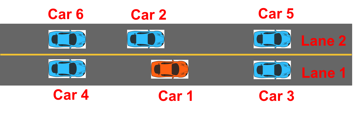
Figure 1. Lane change initial scenario

⬇

void LaneChangeController (Car car1) {

if (genSwitchExp(car1)) { /* go straight */

car1.a = ??_r;

car1.$\theta$ = 0;

} else if (genSwitchExp(car1)) { /* turn left */

car1.a = ??_r;

car1.$\theta$ = ??_r;

} else if (genSwitchExp(car1)) { /* turn right */

car1.a = ??_r;

car1.$\theta$ = ??_r;

} else if (genSwitchExp(car1)) { /* go straight */

car1.a = ??_r;

car1.$\theta$ = 0;

} else { /* rest state */

car1.a = 0;

car1.$\theta$ = 0; }}

generator bool genSwitchExp(Car car1) {

if (??_b) return car1.x $\leq$ ??_r;

else if (??_b) return car1.x $\geq$ ??_r;

else if (??_b) return car1.y $\leq$ ??_r;

else return car1.y $\geq$ ??_r; }

Figure 2. Template for the lane change controller.

⬇

LaneChangeSpec (Car car1, World w) {

for (int i = 0; i < 50; i++) {

LaneChangeController(car1);

MoveCar(car1);

MoveWorld(w);

assert (!DetectCollision(car1, w));

}

assert (ReachedGoal(car1, w)); }

Figure 3. Specification for the lane change synthesis task.

Solving this problem is a significant challenge for three reasons. First, the five-mode controller program is simulated 50 times in the specification, so there are $8\times 10^{34}$ paths in the synthesized program. Moreover at each timestep, DetectCollision has to check for collisions against each of 5 other cars, and each of these checks has to consider 8 separate conditions that can indicate a collision between two cars, so there are a total of 2000 checks. Second, this sketch has 12 Boolean unknowns and 22 real unknowns, so there is a very large space to search. Finally, we use a bicycle-model for the dynamics of the car. Even though this model is simpler than dynamics of a real car, it is still fairly complex and involves non-linear functions such as sine, cosine, and square root.

Because of the these challenges, existing approaches do not perform well on this synthesis task. Many SMT solvers such as Z3 do not provide full support for non-linear real arithmetic and hence, cannot synthesize this program. We also found that dReal, an SMT solver for reals, is unable to solve this problem (see Section 4). On the other hand, smoothing approaches also fail because of the amount of boolean structure in the problem. For comparison, the most complex problem that was solved by the system in (Chaudhuri and Solar-Lezama, 2010) was similar to this one, but involved only 1 obstacle (not 5), with 2 collision conditions (instead of 8), and only scaled to 35 time steps. The use of automatic differentiation helps, but in Section 4, we show that for this benchmark, a smoothing approach with automatic differentiation cannot find a solution even with 300 trials from random initial points (which took about 40 minutes). However, despite all these difficulties, ReaS can synthesize a correct program in 11 minutes.

2.2. The ReaS Approach

We, now, describe the key ideas of the algorithm in the context of the example below. The example looks contrived because it was engineered to highlight all the key features of the algorithm.

Example 2.2.

⬇

float x₁ = ??_r;

assert(-20 $\leq$ x₁ $\leq$ 6);

float a = x₁-5;

if (x₁ $\leq$ 4) a = 6- x₁;

if (x₁ $\leq$ 2) a = 8- x₁;

if (x₁ $\leq$ 0) a = 21+ x₁;

assert(a $\leq$ 0 || a > 25);

SMT Solving Background.

To understand why an SMT solver would do a suboptimal job solving for a value of $x_{1}$ in the program above, it is important to understand how an SMT solver works. As a first step, the program above would be converted into a logical formula that would then be separated into a boolean skeleton and a conjunction of constraints in a theory.

In the example above, the solver would generate boolean variables corresponding to each of the constraints in the theory.

$$\begin{array}[]{lll}y_{1}=x_{1}\leq 0&y_{2}=x_{1}\leq 2&y_{3}=x_{1}\leq 4\\ y_{4}=a\leq 0&y_{5}=a>25&y_{6}=-20\leq x_{1}\leq 6\\ t_{1}=(a_{0}=x_{1}-5)&t_{2}=(a_{1}=6-x_{1})&t_{3}=(a_{2}=8-x_{1})\\ t_{4}=(a_{3}=21+x_{1})&t_{5}=(a_{4}=a_{1})&t_{6}=(a_{4}=a_{0})\\ t_{7}=(a_{5}=a_{2})&t_{8}=(a_{5}=a_{4})&t_{9}=(a=a_{3})\\ t_{10}=(a=a_{5})&&\\ \end{array}$$

The names $a_{0}$ to $a_{5}$ correspond to the temporary values of $a$ at each step of the computation. The boolean constraints include constraints corresponding to the initial assertions in the program (just $y_{6}\wedge(y_{4}\vee y_{5})$), as well as constraints that describe the control flow, shown below:

$$\begin{array}[]{l}t_{1}\wedge t_{2}\wedge t_{3}\wedge t_{4}\wedge(y_{3}\Rightarrow t_{5})\wedge(\overline{y_{3}}\Rightarrow t_{6})\\ (y_{2}\Rightarrow t_{7})\wedge(\overline{y_{2}}\Rightarrow t_{8})\wedge(y_{1}\Rightarrow t_{9})\wedge(\overline{y_{1}}\Rightarrow t_{10})\end{array}$$

Breaking the problem in this manner allows for a clean separation between boolean reasoning which is the responsibility of a SAT solver and theory reasoning, but it deprives the theory solver for crucial information about the control flow structure of the program. In the worst case, the SMT solver has to invoke the theory solver once for every path in the program. Lazy SMT solvers deploy many strategies to avoid the exponential number of calls. In the example above, a good solver solver would be able to generate theory propagation lemmas that show, for example, that $y_{1}$ implies $y_{2}$, which would prevent it from considering infeasible paths, but even then, in the worst case the solver would still have to invoke the theory solver for each of the cases $x_{1}\in[-20,0],(0,2],(2,4],(4,6]$. When you have complex non-linear arithmetic, generating those theory propagation lemmas is much more challenging. For example, if condition $y_{1}$ were instead $x_{1}^{3}+8x_{1}^{2}-28x_{1}<80$, the program would be semantically equivalent to the one above, but it would be much harder for an SMT solver to avoid having to perform exponentially many calls to the theory solver.

The problem is even worse for a program like the one in Example 2.1, with its $10^{34}$ possible paths and with complex non-linear relationships between the branches in different iterations.

Numerical optimization with Smoothing.

The first important feature of ReaS is the ability to use numerical optimization by performing automatic differentiation on a smooth approximation of the program. Figure 4(a) shows the graph for $a$ as function of $x_{1}$ and Figure 4(b) shows its smooth approximation. What jumps out from the graph is that while the branches do introduce discontinuities, the function is still very amenable to numerical optimization. However, numerical optimization can introduce its own problems. For example, even with the ability to smooth away discontinuities and automatically compute derivatives for the whole program, it is clear from the figure that gradient-based optimization will only succeed if it starts at $x_{1}>0$. Otherwise, the algorithm will be stuck on a local minima. In this example, initializing numerical search uniformly at random on the allowed range of $x_{1}$ would give a $77\%$ probability of failing with a local minima, which is already bad, but it is not hard to see how a small change to the program could make this probability arbitrarily close to 100%. Smoothing can ameliorate the problems inherent in numerical search, but cannot eliminate them altogether.

Using SAT solver to eliminate local solutions.

The ReaS approach is to turn the SMT paradigm on its head. In SMT, the SAT solver always has an abstraction of the complete problem. The theory solver helps refine this abstraction, and checks candidate assignments for consistency with the theory, but the SAT solver is the one driving the process. In ReaS, the numerical solver is the one that drives the process. In the beginning, the numerical solver has a smooth approximation of the entire program and uses automatic differentiation and numerical optimization to find a local optima. In the case of the example, that first iteration of gradient descent is likely to converge to the local optima at $x=-20$ which fails to satisfy the constraint. When this happens, ReaS asks the SAT solver for a boolean assignment that is used to guide the search; for example, the SAT solver may suggest setting $y_{1}=x_{1}\leq 0$ to $false$. At this point, the numerical solver performs a new round of numerical optimization, but now under the assumption that $x_{1}>0$, and therefore with one fewer branch compared to the previous case. In this case, setting this boolean condition is sufficient to steer the numerical optimization to a region where it can converge to a value that satisfies the constraint.

Once the numerical solver finds a solution that satisfies the constraints, say $x=4.01$, it still needs to check that it really satisfies the boolean constraints and that it is a true solution and not an artifact of the smoothing transformation. It does this by suggesting assignments to the SAT solver corresponding to that solution; in this case $\overline{y_{1}},\overline{y_{2}},\overline{y_{3}},y_{4},\overline{y_{5}}$. As the SAT solver sets these variables and checks them against the boolean constraints, the numerical solver checks that the current solution is still valid when the respective branches have been fixed in the program. As a result, the SAT solver helps refine the solution provided by the numerical solver, until a precise solution to the overall problem has been produced.

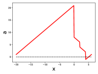
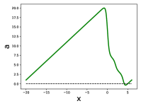
(a)	(b)

Figure 4. (a) Graph showing $a$ vs $x_{1}$ in Example 2.2. (b) Its smooth approximation.

3. The ReaS Intermediate Representation

The core language (L) of ReaS is shown below. The language consists of real-valued expressions $E$, Boolean expressions $B$ and Boolean unknowns $H$. The real-valued expressions can either be a real unknown $x$, a constant $c$, a real-valued operation op such as addition, multiplication, sine, cosine, etc, or a if-then-else expression ite. The Boolean expressions can either be a comparison $E\geq 0$, a conjunction, or a negation. There are two kinds of ite expressions in the language–one where the conditional is a Boolean expression and the other where the conditional is a Boolean unknown because they are treated differently for the numerical problem. The language does not allow Boolean unknowns to appear anywhere other than as a conditional. However, this does not decrease the expressive power of the language since those cases can be reduced to the core language easily. The imperative programs shown in Section 2 can be converted into this core language using straight-forward transformation passes and loop unrolling.

$$E := x\;|\;c\;|\;\text{op}(\{E_{i}\}_{i})\;|\;\text{ite}(B,E_{1},E_{2})\;|\;\text{ite}(H,E_{1},E_{2})$$

$$B := E\geq 0\;|\;B_{1}\wedge B_{2}\;|\;\neg B$$

$$H := y$$

The semantics of some features of the language is shown below. It is defined in terms of a mapping $\sigma$ from the unknowns to actual values.

$$\llbracket x\rrbracket_{\sigma} := \sigma[x]$$

$$\llbracket y\rrbracket_{\sigma} := \sigma[y]\hskip 28.45274pt//~{}\{0,1\}$$

$$\llbracket E_{1}+E_{2}\rrbracket_{\sigma} := \llbracket E_{1}\rrbracket_{\sigma}+\llbracket E_{2}\rrbracket_{\sigma}$$

$$\llbracket\text{ite}(B,E_{1},E_{2})\rrbracket_{\sigma} := \llbracket B\rrbracket_{\sigma}.\llbracket E_{1}\rrbracket_{\sigma}+\llbracket\neg B\rrbracket_{\sigma}.\llbracket E_{2}\rrbracket_{\sigma}$$

$$\llbracket E\geq 0\rrbracket_{\sigma} := \llbracket E\rrbracket_{\sigma}\geq 0$$

3.1. Synthesis Problem

The synthesis problem is given a program $P=\text{assert}(B_{1},\cdots,B_{k})$, find $\sigma$ such that $\forall k.\llbracket B_{k}\rrbracket_{\sigma}=1$. For now on, we will use $\psi(\sigma)$ to represent this predicate. So, the synthesis problem is to solve the formula: $\exists\sigma.~{}\psi(\sigma)$.

ReaS divides the synthesis problem into a SAT part ($\psi_{B}$) and a numerical part ($\psi_{N}$). We, first, describe the abstraction process for producing $\psi_{B}$ and $\psi_{N}$ and Section LABEL:sec:solver describes the algorithm to solve $\psi$ by repetitively solving $\psi_{B}$ and $\psi_{N}$.

3.2. Boolean Abstraction ($\alpha_{B}$)

The Boolean abstraction is obtained similar to the process used in SMT solvers. Concretely, the language for Boolean constraints ($L_{B}$) is:

$$\widetilde{P_{B}} := \text{assert}(\widetilde{B}_{1},\cdots,\widetilde{B}_{k})$$

$$\widetilde{B} := y\;|\;\widetilde{B}_{1}\wedge\widetilde{B}_{2}\;|\;\neg\widetilde{B}$$

The language is almost same as the $B$ expressions in the original language. The only exception is that the term $E\geq 0$ is now replaced by Boolean unknowns.

The Boolean abstraction, $\alpha_{B}$, is a function from $L$ to $L_{B}$ and is defined as below:

$$\alpha_{B}(y) = y$$

$$\alpha_{B}(E\geq 0) = \text{Create new }y$$

$$\alpha_{B}(B_{1}\wedge B_{2}) = \alpha_{B}(B_{1})\wedge\alpha_{B}(B_{2})$$

$$\alpha_{B}(\neg B) = \neg\alpha_{B}(B)$$

3.3. Numerical Abstraction ($\alpha_{N}$)

We now describe the abstraction process to produce $\psi_{N}$ from $\psi$. The abstraction is defined with respect to a function $I$, called interface mapping, that maps every Boolean expression in $\psi$ to one of $\{0,1,\bot\}$. $I(B_{i})=v_{i}\neq\bot$ means that the Boolean expression $B_{i}$ should have the value $v_{i}$. If $v_{i}=\bot$, then the value is not yet set. The interface mapping specializes a synthesis problem defined by $\psi$ to

$$\exists\sigma.~{}\psi[\{B_{k}/v_{k}\}_{k}](\sigma)\wedge_{i}\llbracket B_{i}[\{B_{k}/v_{k}\}_{k\neq i}]\rrbracket_{\sigma}=v_{i}$$

where the spec $\psi$ is first simplified by substituting the expressions $B_{k}$ with the values $v_{k}=I(B_{k})$ when $v_{k}\neq\bot$, and additional constraints are added to ensure that $\sigma$ satisfies the assignments in $I$.

The goal of the numerical abstraction ($\alpha_{N}$) is to produce a smooth approximation $\psi_{N}$ of the specialized problem above that can be fed to an off-the-shelf numerical solver to find an assignment to $\sigma$ if one exists. Note that unlike the SMC approach, ReaS does not require $\psi_{N}$ to be composed of linear/convex functions. However, we want $\psi_{N}$ to be smooth and continuous because numerical algorithms perform poorly in the presence of discontinuities. The main source of discontinuity arises when the Boolean expression in an ite or a conjunction is not yet set by $I$. ReaS eliminates these discontinuities by performing a program transformation that replaces the sharp transitions with smooth transition functions such as sigmoid as described in the next subsection.

3.3.1. Abstraction rules

The language for numerical constraints ($L_{N}$) in ReaS is shown below. At the top level, we have a conjunction of numerical inequalities $(\widetilde{E}_{i}\geq 0)$ where $\widetilde{E}$ is again similar to $E$ in the original language minus the ite expression.

$$\widetilde{P_{E}} := \widetilde{E}_{1}\geq 0\wedge\cdots\wedge\widetilde{E}_{n}\geq 0$$

$$\widetilde{E} := x\;|\;c\;|\;\text{op}(\{\widetilde{E}_{i}\}_{i})$$

Note that there are numerical algorithms (such as sequential quadratic programming) that take in a conjunction of inequalities and perform constrained optimization on them directly. Even for numerical algorithms that can only perform unconstrained optimization (such as plain gradient descent), it is easy to transform a conjunction of inequalities into a smooth objective function.

Given a program $P=\text{assert}(B_{1},\cdots,B_{k})$ in $L$, the goal of the abstraction is to produce a program $\widetilde{P_{E}}$ in $L_{N}$. In order to do that, we define a transformation rule $e\xrightarrow{I}(\widetilde{e},p)$ where $e$ is an expression in $L$ (either an $E$ or a $B$ expression), $\widetilde{e}$ is the corresponding expression in $L_{N}$, and $p$ is the conjunction of numerical constraints obtained so far. This formulation allows us to collect numerical constraints from intermediate expressions if necessary. The transformation is defined in terms of two parameters: $(\beta,\epsilon)$. $\beta$ is the smoothing parameter that controls how smooth the approximation should be. Higher values for $\beta$ mean less smoothing. $\epsilon$, a small positive constant, is the precision of numerical calculation that arises due to im-precise floating point computation. Because of this, the expression $\widetilde{E}\geq 0$ in $L_{N}$ actually means $\widetilde{E}\geq-\epsilon$.

The rules for performing the abstraction for expressions in the language are shown in Figure 5. We first focus on the rules for expressions other than ite and conjunction expressions. For an $E$ expression, the abstraction produces an $\widetilde{E}$ that smoothly approximates the original expression. For simple cases such as a real unknown and constant, the abstraction just returns the same expression as shown in the RHOLE and CONST rules. In this case, there are no intermediate constraints and hence, $p$ is just true (T). For an op expression, the OP rule recursively smooths the expressions in its arguments and then creates a new op expression with these smoothed replacements and concatenates the intermediate constraints obtained from abstracting the arguments. ReaS assumes that op is itself a smooth and continuous operation. For operations like division or $sqrt$ that are not defined for all inputs, we replace them with continuous approximations, and rely on the frontend to introduce assertions that ensure their inputs stay away from the regions where the approximations differ significantly from the true operations.

In order to understand the abstraction rules for the $B$ expressions, we first define a function called P-distance.

Definition 3.1 (P-distance).

The P-distance (short for positive-distance) for a Boolean expression $b$ in $L$ is a function ${\mathcal{P}_{d}}$ that takes in an assignment to the unknowns $\sigma$ and produces a real value such that $\forall\sigma.~{}({\mathcal{P}_{d}}(\sigma)\geq\epsilon\implies\llbracket b\rrbracket_{\sigma}=1)\wedge({\mathcal{P}_{d}}(\sigma)\leq-\epsilon\implies\llbracket b\rrbracket_{\sigma}=0)$. Thus, for numerical purposes, we can assume $b\approx{\mathcal{P}_{d}}\geq 0$. There can be more than one P-distance function for the same Boolean expression.

The abstraction rule for a $B$ expression in $L$ produces an $\widetilde{E}$ expression that is a smooth approximation to a P-distance function for $B$. For example, for $e\geq 0$, the natural choice for its P-distance function is $e$ itself. So, the rule GE first computes the smooth approximation of $e$. For Boolean expressions, the rules also need to take into account whether there is a value assigned to them in the $I$ mapping. This is done using the MatchNUpdate function which takes in the smoothed expression $\widetilde{e}$ and the value $v$ from $I$. Then, it checks for one of the three cases: 1. if $v=\bot$, it means that the value is not yet set and hence, there is no update and no new constraints, 2. if $v=1$, then the expression $\widetilde{e}$ is replaced with a large positive constant ($K=100$) and a new constraint $\widetilde{e}\geq 0$ is added, and 3. if $v=0$, then similar to case 2, the expression $\widetilde{e}$ is replaced with a large negative constant and the condition $-\widetilde{e}\geq 0$ is added . The reason for replacing $\widetilde{e}$ with constants in cases 2 and 3 is so that other expressions that depend on $\widetilde{e}$ can infer the Boolean value of the $B$ expression it represents without any ambiguity (because of the large magnitude of these constants). The NOT rule for the $\neg b$ expression, similarly, first computes the abstraction for $b$ and negates the expression obtained to get a smooth approximation to a P-distance for $\neg b$.

Finally, the abstraction for the assert expression iteratively smooths each of its $b$ arguments and creates the final set of numerical constraints $\widetilde{P_{E}}$ to form the numerical problem $\psi_{N}$. This final set of constraints is the conjunction of the constraints obtained after transforming each Boolean argument ($p_{i}$) and as well as constraints to ensure that the abstraction of each Boolean argument ($\widetilde{e}_{i}$) is greater than $0$.

Example 3.2.

Consider the program $P=\text{assert}(\text{ite}(x_{1}\geq 0,x_{2},x_{3})\geq 0)$ where $x_{1},x_{2},x_{3}$ are real unknowns and let $I(x_{1}\geq 0)=0$. The abstraction for $x_{1}\geq 0$ results in $(-100,-x_{1}\geq 0)$. So, the ite expression can be thought as $\text{ite}(-100\geq 0,x_{2},x_{3})$. Even though we have not yet discussed the rule for abstracting ite expressions, in this case, it is clear that the abstraction should just produce $x_{3}$. Overall, abstracting $P$, in this example, will result in $\widetilde{P_{E}}=x_{3}\geq 0\wedge-x_{1}\geq 0$.

$$\text{ASSERT}~{}~{}~{}\frac{\begin{array}[]{c}b_{1}~{}~{}\xrightarrow{I}~{}~{}(\widetilde{e}_{1},p_{1})~{}\cdots~{}b_{k}~{}~{}\xrightarrow{I}~{}~{}(\widetilde{e}_{k},p_{k})\\ p=p_{1}\wedge\cdots\wedge p_{k}\wedge(\widetilde{e}_{1}\geq 0)\cdots\wedge(\widetilde{e}_{k}\geq 0)\end{array}}{\begin{array}[]{c}\text{assert}(b_{1},\cdots,b_{k})~{}~{}\xrightarrow{I}~{}~{}(0,p)\end{array}}$$

$$\text{GE}~{}~{}~{}\frac{\begin{array}[]{c}e~{}~{}\xrightarrow{I}~{}~{}(\widetilde{e},p)\\ (\widetilde{e}_{I},p_{I})=\textsc{MatchNUpdate}(\widetilde{e},I(e\geq 0))\\ \end{array}}{\begin{array}[]{c}e\geq 0~{}~{}\xrightarrow{I}~{}~{}(\widetilde{e}_{I},p\wedge p_{I})\end{array}}$$

$$\text{NOT}~{}~{}~{}\frac{\begin{array}[]{c}b~{}~{}\xrightarrow{I}~{}~{}(\widetilde{e},p)\\ (\widetilde{e}_{I},p_{I})=\textsc{MatchNUpdate}(-\widetilde{e},I(\neg b))\end{array}}{\begin{array}[]{c}\neg b~{}~{}\xrightarrow{I}~{}~{}(\widetilde{e}_{I},p\wedge p_{I})\end{array}}$$

$$\text{AND}~{}~{}~{}\frac{\begin{array}[]{c}b_{1}~{}~{}\xrightarrow{I}~{}~{}(\widetilde{e}_{1},p_{1})\qquad b_{2}~{}~{}\xrightarrow{I}~{}~{}(\widetilde{e}_{2},p_{2})\\ \widetilde{e}=\widetilde{e}_{1}*t+\widetilde{e}_{2}*(1-t),~{}~{}t=\mathcal{F}_{s}(\widetilde{e}_{2}-\widetilde{e}_{1})\\ (\widetilde{e}_{I},p_{I})=\textsc{MatchNUpdate}(\widetilde{e},I(b_{1}\wedge b_{2}))\end{array}}{\begin{array}[]{c}b_{1}\wedge b_{2}~{}~{}\xrightarrow{I}~{}~{}(\widetilde{e}_{I},p_{1}\wedge p_{2}\wedge p_{I})\end{array}}$$

$${\displaystyle\text{RHOLE}~{}~{}~{}\frac{\begin{array}[]{c}{}\hfil\end{array}}{\begin{array}[]{c}x~{}~{}\xrightarrow{I}~{}~{}(x,\leavevmode\lstinline{{\lst@@@set@language\lst@@@set@numbers\lst@@@set@frame\lst@@@set@rulecolor\lst@@@set@language\lst@@@set@numbers\small{\@listingGroup{ltx_lst_identifier}{T}}}}})\end{array}}$$

$${\displaystyle\text{CONST}~{}~{}~{}\frac{\begin{array}[]{c}{}\hfil\end{array}}{\begin{array}[]{c}c~{}~{}\xrightarrow{I}~{}~{}(c,\leavevmode\lstinline{{\lst@@@set@language\lst@@@set@numbers\lst@@@set@frame\lst@@@set@rulecolor\lst@@@set@language\lst@@@set@numbers\small{\@listingGroup{ltx_lst_identifier}{T}}}}})\end{array}}$$

$$\text{OP}~{}~{}~{}\frac{\begin{array}[]{c}e_{i}~{}~{}\xrightarrow{I}~{}~{}(\widetilde{e}_{i},p_{i})\end{array}}{\begin{array}[]{c}\text{op}(\{e_{i}\}_{i})~{}~{}\xrightarrow{I}~{}~{}(\text{op}(\{\widetilde{e}_{i}\}_{i}),\underset{i}{\wedge}p_{i})\end{array}}$$

$$\text{ITE1}~{}~{}~{}\frac{\begin{array}[]{c}e_{1}~{}~{}\xrightarrow{I}~{}~{}(\widetilde{e}_{1},p_{1})\qquad e_{2}~{}~{}\xrightarrow{I}~{}~{}(\widetilde{e}_{2},p_{2})\\ b~{}~{}\xrightarrow{I}~{}~{}(\widetilde{e}_{c},p_{c})\\ \widetilde{e}=\widetilde{e}_{1}*\mathcal{F}_{s}(\widetilde{e}_{c})+\widetilde{e}_{2}*(1-\mathcal{F}_{s}(\widetilde{e}_{c}))\end{array}}{\begin{array}[]{c}\text{ite}(b,e_{1},e_{2})~{}~{}\xrightarrow{I}~{}~{}(\widetilde{e},p_{1}\wedge p_{2}\wedge p_{c})\end{array}}$$

$${\displaystyle\text{BHOLE1}~{}~{}~{}\frac{\begin{array}[]{c}v=I(y)\neq\bot\end{array}}{\begin{array}[]{c}y~{}~{}\xrightarrow{I}~{}~{}(v,\leavevmode\lstinline{{\lst@@@set@language\lst@@@set@numbers\lst@@@set@frame\lst@@@set@rulecolor\lst@@@set@language\lst@@@set@numbers\small{\@listingGroup{ltx_lst_identifier}{T}}}}})\end{array}}$$

$$\text{BHOLE2}~{}~{}~{}\frac{\begin{array}[]{c}I(y)=\bot\\ x=\text{Create new real unknown for }y\\ p=(x\geq 0)\wedge(1-x\geq 0)\\ p=p\wedge(\delta-x(1-x)\geq 0)\end{array}}{\begin{array}[]{c}y~{}~{}\xrightarrow{I}~{}~{}(x,p)\end{array}}$$

$$\text{ITE2}~{}~{}~{}\frac{\begin{array}[]{c}e_{1}~{}~{}\xrightarrow{I}~{}~{}(\widetilde{e}_{1},p_{1})\qquad e_{2}~{}~{}\xrightarrow{I}~{}~{}(\widetilde{e}_{2},p_{2})\\ y~{}~{}\xrightarrow{I}~{}~{}(\widetilde{e}_{c},p_{c})\\ \widetilde{e}=\widetilde{e}_{1}*\widetilde{e}_{c}+\widetilde{e}_{2}*(1-\widetilde{e}_{c})\\ \end{array}}{\begin{array}[]{c}\text{ite}(y,e_{1},e_{2})~{}~{}\xrightarrow{I}~{}~{}(\widetilde{e},p_{1}\wedge p_{2}\wedge p_{c})\end{array}}$$

$${\displaystyle\textsc{MatchNUpdate}(\widetilde{e},v)=\begin{cases}(\widetilde{e},\leavevmode\lstinline{{\lst@@@set@language\lst@@@set@numbers\lst@@@set@frame\lst@@@set@rulecolor\lst@@@set@language\lst@@@set@numbers\small{\@listingGroup{ltx_lst_identifier}{T}}}}}),&\text{if}\ v=\bot\\ (K,(\widetilde{e}\geq 0)),&\text{if}\ v=1\\ (-K,(-\widetilde{e}\geq 0)),&\text{if}\ v=0\end{cases}$$

Figure 5. Numerical abstraction rules. T stands for true, $K$ is a large positive constant (100) and $\delta$ is a small positive constant. Note that expressions such as $e_{1}*e_{2}$ are symbolic expressions. $\mathcal{F}_{s}$ is a smooth transition function.

Now, we can look at the rules for expressions that introduce discontinuities i.e. if-then-else and conjunctions.

If-then-else

Let us first consider the ite expression of the form $\text{ite}(b,e_{1},e_{2})$ that has a Boolean expression as the condition. The rule ITE1 describes the abstraction for these expressions. The rule first recursively smooths the expressions $e_{1}$ and $e_{2}$ resulting in expressions $\widetilde{e}_{1}$ and $\widetilde{e}_{2}$. Then, the condition $b$ is also transformed to produce the approximation for its P-distance function $\widetilde{e}_{c}$. If we were to use the actual semantics of the ite expression, we would get $\widetilde{e}_{1}*(\widetilde{e}_{c}\geq 0)+\widetilde{e}_{2}*(1-(\widetilde{e}_{c}\geq 0))$. Note that the operations +, * in the above expression are actually symbolic operations. Clearly, the function $\widetilde{e}_{c}\geq 0$ has a discontinuity at $\widetilde{e}_{c}=0$. To overcome this discontinuity, the ITE1 rule replaces $\widetilde{e}_{c}\geq 0$ with $\mathcal{F}_{s}(\widetilde{e})$ where $\mathcal{F}_{s}$ is a smooth transition function:

$$\mathcal{F}_{s}(x)=\text{sigmoid}_{\beta}(x)=\frac{1}{1+e^{-\beta x}}$$

The rule ITE2 describes the abstraction for expressions of the form $\text{ite}(y,e_{1},e_{2})$. In this case, $y$ is abstracted using the BHOLE1 or the BHOLE2 rule. In the case where $I$ already fixes the value of $y$ to $1$ or $0$, the ite expression will be simplified to just $\widetilde{e}_{1}$ or $\widetilde{e}_{2}$ respectively. If the value of $y$ is not yet set, then the rule BHOLE2 creates a new real unknown $x$ corresponding to $y$. This new variable is constrained to be in the interval $[0,1]$. In addition, the constraint $x(1-x)\leq\delta$ where $\delta=0.1/\beta$ is added to enforce that $x$ is either close to $0$ or $1$. The ite expression is, then, abstracted by a linear combination of $\widetilde{e}_{1}$ and $\widetilde{e}_{2}$ such that when $x=1$, the abstraction will result in $\widetilde{e}_{1}$ and when $x=0$, the result will be $\widetilde{e}_{2}$.

Conjunctions

The rule for abstracting a conjunction of two Boolean expressions is based on the following lemma:

Lemma 3.3.

Let ${\mathcal{P}_{d}}_{1}$ and ${\mathcal{P}_{d}}_{2}$ be the P-distance functions for Boolean expressions $b_{1}$ and $b_{2}$. Then, ${\mathcal{P}_{d}}=\text{min}({\mathcal{P}_{d}}_{1},{\mathcal{P}_{d}}_{2})$ is a P-distance function for $b_{1}\wedge b_{2}$.

Based on the lemma, the AND rule first gets the abstractions of $b_{1}$ and $b_{2}$ and then smooths the min of the results. The smoothing is done by rewriting $\text{min}(\widetilde{e}_{1},\widetilde{e}_{2})$ as $\text{ite}(\widetilde{e}_{2}-\widetilde{e}_{1}\geq 0,\widetilde{e}_{1},\widetilde{e}_{2})$ and applying the ITE1 rule.

3.3.2. Computing gradients

One of the advantages of our numerical abstraction algorithm is that once the smoothed program $\widetilde{P_{E}}$ is produced, we can use automatic differentiation (Naumann, 2010) to symbolically compute the gradients necessary to perform gradient-based numerical search. For example, consider the expression $e=e_{1}*e_{2}+e_{3}$ with two unknowns $x=[x_{1},x_{2}]$ and let $\sigma$ be an assignment to the unknowns. Since there are two unknowns, each sub-expression will have two gradients, i.e. $\Gamma(e,\sigma)=\left[\left(\frac{\partial e}{\partial x_{1}}\right)_{\sigma},\left(\frac{\partial e}{\partial x_{2}}\right)_{\sigma}\right]$ where $\Gamma$ is the notation used to get the gradients for any sub-expression $e$ at the assignment $\sigma$. Automatic differentiation applies the chain rule repeatedly to each elementary expression i.e. in the above example

$$\Gamma(e,\sigma)=\llbracket e_{2}\rrbracket_{\sigma}*\Gamma(e_{1},\sigma)+\llbracket e_{1}\rrbracket_{\sigma}*\Gamma(e_{2},\sigma)+\Gamma(e_{3},\sigma)$$

This process allows us to calculate the gradients accurately and in time that is proportional to the time it takes to evaluate an expression.

3.4. Properties of Numerical Abstraction

Let $e$ be the original expression, $\widetilde{e}$ be the result of the abstraction and let $x$ be the set of unknown reals in $\widetilde{e}$, then the following theorems hold for any $I$.

Theorem 3.4 (Continuity).

$\widetilde{e}$ is continuous with respect to $x$ under the assumption that all op operations in $e$ are continuous with respect to their operands.

Theorem 3.5 (Differentiability).

$\frac{\partial\widetilde{e}}{\partial x}$ is continuous with respect to $x$ under the assumption that all op operations in $e$ are differentiable with respect to their operands.

Theorem 3.6 (Closeness).

$\underset{\beta\rightarrow\infty}{lim}e\approx\widetilde{e}$

This theorem states that when $\beta\rightarrow\infty$, both $e$ and its abstraction $\widetilde{e}$ agree on almost all assignments to the unknowns. We say almost because $e$ and $\widetilde{e}$ may not agree at the branching points. For example, consider $\text{ite}(x\geq 0,1,0)$. In this case when $x=0$, the abstraction will have undefined behavior.

4. Evaluation

In this section, we evaluate ReaS on 5 case-studies involving hybrid systems. In particular, we focus on answering the following questions: (1) Can ReaS solve complex synthesis problems that involve a combination of discrete and continuous reasoning? (2) How does it compare with only smoothing techniques? (3) How does it compare with existing SMT solvers and mixed integer approaches?

Experimental Setup

ReaS uses the SNOPT software (Gill et al., 2005) for performing numerical optimization. SNOPT uses sequential quadratic programming and can handle constrained optimization better than standard gradient descent techniques. For the SAT solver, we took the MiniSAT solver and modified it as described in Section LABEL:sec:solver. All experiments are run on a machine using 2.4GHz Intel i5 core with 8GB RAM.

	Stats					ReaS					only smoothing
Benchmarks	#$y$	#$x$	#I	#B	#A	Time(s)			#N	#R	#S	#C	$T_{C}$
						20%	median	80%
LaneChange	12	22	50	11455	2350	276s	634s	1261s	94	4	9/300	0/300	> 2500s
QuadObstacle	4	38	70	1753	1714	81s	217s	822s	16	1	34/300	21/300	857s
QuadLanding	6	44	60	1567	1413	231s	374s	637s	32	2	62/300	22/300	665s
ParallelPark	9	15	100	11204	1904	354s	630s	870s	98	5	0/300	0/300	> 2100s
Thermostat	0	2	500	30908	2100	78s	175s	280s	31	3	21/300	19/300	220s

Figure 6. Benchmarks statistics and results. #$y$: number of Boolean holes, #$x$: number of real holes, #I: number of iterations used in the simulation, #B: number of Boolean expressions, #A: number of assertions, #N: number of calls to numerical solver, #R: number of restarts of SAT solver, #S: number of times a solution is found, #C: number of times a correct solution is found and $T_{C}$ is the expected time for the only smoothing approach to find a solution with 90% confidence.

4.1. Benchmarks

Apart from the lane changing example in Section 2, we used ReaS to synthesize two benchmarks involving a 1-dimensional quad-copter, the parallel parking benchmark from (Chaudhuri and Solar-Lezama, 2012), and the thermostat benchmark from (Jha et al., 2010). Figure 6 lists the 5 benchmarks together with some statistics such as the number of Boolean and real unknowns, the number of iterations the controller (to be synthesized) is simulated in the specification, and the total number of Boolean expressions and assertions. Full benchmark problems along with the demos of the synthesized solutions can be found in the supplementary material.

Quadcopter obstacle avoidance

The task is to synthesize a controller to perform the maneuver shown in Figure 7 without colliding with the obstacle. The program with unknowns for this controller is shown in Figure 8. This controller has three modes where each mode uses a proportional-derivative (PD) controller to set the forces that need to be generated by the two rotors of a simplified 1-D quadcopter. The synthesizer is required to find the switching conditions (which are based on the position of the copter similar to the lane change benchmark) as well as the parameters of the PD controllers for the different modes. Note that, in this case, a single PD controller is not sufficient to perform the task and hence, it is necessary to compose multiple PD controllers as shown in the template. The synthesizer is also required to find the values of the intermediate desired states for the PD controllers.

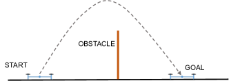
Figure 7. Quadcopter obstacle avoidance scenario.

⬇

void Controller(Copter c) {

if (genSwitchExp(c)) { /* mode 1 */

genPDController(c);

} else if (genSwitchExp(c)) { /* mode 2 */

genPDController(c);

} else { /* mode 3 */

genPDController(c);

}

}

generator void genPDController(Copter c) {

F = (c.y - ??_r)*??_r + (c.vel.y - ??_r)*??_r;

bias = (c.ang - ??_r)*??_r + (c.angvel - ??_r)*??_r

+ (c.x - ??_r)*??_r + (c.vel.x - ??_r)*??_r;

c.left_force = F + bias;

c.right_force = F;

}

Figure 8. Program with unknowns for quadcopter controller.

Quadcopter landing

Using the same template shown in Figure 8, but with different specifications, it is possible to synthesize controllers for achieving other goals. In this benchmark, we synthesize a controller for landing a quadcopter gracefully. The copter starts at a position above the ground with an initial thrust that imbalances the copter and target is to reach a position on the ground without crashing. There are no obstacles (other than the ground) in this case, but the synthesizer still needs to figure out how to compose the different PD controllers to achieve the goal.

Parallel parking

This benchmark synthesizes a controller to parallel park a car as described in (Chaudhuri and Solar-Lezama, 2012) (a tool based on the smooth interpretation work (Chaudhuri and Solar-Lezama, 2010)). The template for this benchmark is similar to the template for the lane changing benchmark. Our template is different from (Chaudhuri and Solar-Lezama, 2012) in two aspects. (Chaudhuri and Solar-Lezama, 2012) uses switching conditions based on time; we replaced them with conditions based on the state of the car since it leads to more robust controllers. (Chaudhuri and Solar-Lezama, 2012) only uses 10 time-steps to do the simulation, but in our template, we decrease the step size and increased the number of simulation steps to 100. This reinforces the fact that our technique scales much better than the smoothing technique that (Chaudhuri and Solar-Lezama, 2012) uses.

Thermostat

The final benchmark is to synthesize the thermostat controller described in (Jha et al., 2010). This thermostat is a state machine with four states: OFF, HEATING, ON and COOLING. The switching conditions for transitioning from HEATING to ON and COOLING to OFF are fixed by the constraints of the thermostat’s heater. The other two switching conditions should be figured out by the synthesizer such that the temperature of the room is maintained between 18^∘C and 20^∘C. In addition to the safety conditions, this benchmark encodes some performance metrics, in particular, it adds minimum dwell time constraints for the OFF and ON phases. The minimum dwell time constraint states that the thermostat should at least be in the state for $T$ seconds before transitioning to the next state. The system in (Jha et al., 2010) takes in these universal constraints (that should be true in every state) and uses a fix-point computation based algorithm to find the switching conditions. In ReaS, we instead specify the problem by simulating the thermostat for 500 time steps with dt = 2s and asserting that the constraints are satisfied at every time step. Most of the SMT solvers choke when given a problem of this magnitude, but ReaS is still able to synthesize it. Figure 9 shows how the room temperature and the state of the thermostat change with a controller that is synthesized with minimum dwell time constraint of 200s for the OFF and ON phases.

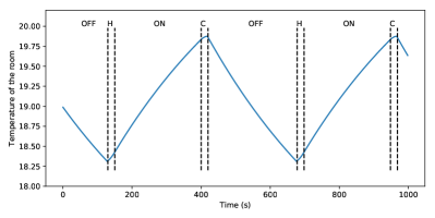
Figure 9. Room temperature vs time for the synthesized thermostat controller.

4.2. Results

Figure 6 shows the evaluation results. The Time column lists the time taken in seconds (20th percentile, median, and 80th percentile) to synthesize the benchmarks in ReaS. This experiment is run with a conflict threshold $\eta=5$ and unlimited RESTART_LIMIT, but with a timeout of 30 minutes. We ran each benchmark 10 times and ReaS is able to synthesize all the benchmarks for all 10 runs within 25 minutes. The #N and #R columns show the median number of numerical iterations and SAT solver restarts taken by these benchmarks.

Next, we performed an experiment to compare ReaS with an only smoothing approach. For each benchmark, we took the numerical abstraction when interface mapping $I$ is empty and ran our numerical solver on this abstraction with a random initial assignment to the unknowns. We ran each benchmark 300 times and collected the number of times the numerical solver is able to converge to a valid solution for the abstraction (shown in #S column in Figure 6). Since, some of the solutions might actually be incorrect on the original problem due to the approximations introduced by smoothing, we also computed the number of times a correct solution is found by the only smoothing approach (shown in #C column). Using these statistics and the average time to run each numerical iteration, we also computed the expected time for the only smoothing approach to find a correct solution with 90% confidence (shown in $T_{C}$ column). The only smoothing approach can synthesize the quadcopter and thermostat benchmarks if the numerical solver is run sufficient number of times, but it is not able to find a correct solution for the lane change and parallel parking benchmarks even with 300 iterations. This shows that searching the numerical space based on the program structure is very important for some of these benchmarks. Note that, in this experiment the comparison is done against the smoothing approach described in this paper and not the smooth interpretation work in (Chaudhuri and Solar-Lezama, 2010).

We also performed an experiment to see how the conflict threshold $\eta$ effects the performance of ReaS. A higher conflict threshold means that the search space of the numerical solver is significantly reduced by the assignments to a higher number of Boolean expressions, which increases the likelihood for the numerical solver to hit the global solution (if there is one in the reduced search space). On the other hand, a higher conflict threshold will result in spending more time to eliminate a truly infeasible partial assignment because the system needs to wait until the conflict threshold is hit. Figure 10 shows the graph for the time as well as the number of numerical iterations required for synthesizing the benchmarks when $\eta=[3,4,5,6,7]$. It can be seen that different benchmarks have different behaviors since the trade-off between the two aspects mentioned above depends on the structure of the benchmark. However, we can see that for any of the small conflict thresholds ($3\leq\eta\leq 7$), the system can synthesize the benchmarks in reasonable time.

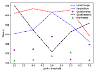
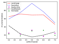
Figure 10. Graphs showing the time and the number of numerical iterations vs the conflict threshold in ReaS.

4.3. Comparison to SMT solvers

We compared ReaS with dReal, a state-of-the-art SMT solver for reals. In-order to do this comparison, we wrote a script to translate the benchmarks written in ReaS into the SMT-lib format and fed them to the dReal solver. However, dReal could not solve any of our benchmarks with a timeout of 60 minutes. We also ran Z3 on the thermostat benchmark (the only benchmark in our suite that does not contain non-linear functions) and found that even Z3 could not solve with a timeout of 60 minutes. These results support our claim that the traditional SMT approaches do not scale for these kinds of synthesis problems.

4.4. Comparison to mixed integer approaches

In the final experiment, we evaluate how the mixed integer approach compares to ReaS. Since most of the mixed integer solvers only handle linear and convex constraints, we created a toy version of the lane change benchmark. We replaced the complex dynamics of the car with a simple point car model that can only either move along the x-direction or the y-direction. To deal with conditionals and disjunctions, we manually translated them to linear constraints using the big-M method. This translation, however, introduces one 0-1 integer variable for each Boolean expression in the original problem and a continuous variable for every conditional. We verified that the translation to the mixed integer format is correct by fixing the values to the unknowns with a solution found by ReaS. We ran this translated version using Gurobi, a state of the art mixed integer solver. However, Gurobi was not able to find a solution with a timeout of 60 minutes, whereas ReaS was able to solve the benchmark in just 3 seconds. This shows that even the mixed integer solvers are not suitable for handling these benchmarks.

5. Related Work

To the best of our knowledge, this paper is the first that achieves both end-to-end differentiability of a program and uses a SAT solver to help perform numerical optimization to find unknowns in a program. However, there are several related works for each of the two pieces.

End-to-end differentiability: The idea of achieving end-to-end differentiability in not new in the neural networks community. The entire back-propagation algorithm is based on this principle. Our idea of smoothing using sigmoids is inspired by the Neural networks’ use of sigmoids in-place of step functions to make the network differentiable. For neural networks, there are libraries such as TensorFlow (Abadi et al., 2016) where users can write their networks in a high-level language and the library can automatically compute the required gradients. In ReaS, we use similar ideas to programmatically smooth conditionals and conjunctions. The recent works on neural Turing machines (Graves et al., 2014) and neural program interpreters (Reed and De Freitas, 2015; Kurach et al., 2015; Neelakantan et al., 2015; Kaiser and Sutskever, 2015) achieve end-to-end differentiability in the presence of discrete structure. They accomplish this by turning the discrete variables into continuous variables for encoding the probabilities of the different discrete options. On the other hand, in this paper, we relax Boolean unknowns to real unknowns in the range [0, 1] and then, use a SAT solver to fix their values. This approach allows us to benefit from the fact that SAT solvers are inherently better at handling discrete problems.

Smoothing in the context of programs is introduced in the smooth interpretation work (Chaudhuri and Solar-Lezama, 2010) and subsequently used in (Chaudhuri et al., 2014) to solve synthesis problems involving Boolean and quantitative objectives. Smoothing using sigmoids that we use in this paper is a simplified version of the smoothing algorithm used in (Chaudhuri and Solar-Lezama, 2010). However, our approach allows us to use automatic differentiation techniques to compute gradients necessary for the numerical optimization.

SAT/SMT solvers: There have been many approaches to SMT solving over real numbers that incorporate numerical methods. Examples include convex optimization algorithms (Borralleras et al., 2009; Nuzzo et al., 2010; Shoukry et al., 2017), interval-based algorithms (Fränzle et al., 2007; Gao et al., 2013b), Bernstein polynomials (Munoz and Narkawicz, [n. d.]), and linearization algorithms (Cimatti et al., 2017). However, these approaches strictly partition the problem into a Boolean part and many of numerical parts that loses the structural dependencies between the numerical parts and hence, they are not able to leverage the benefits of doing numerical optimization on the entire problem.

ReaS’s modifications to the SAT solver to support soft learnts and suggestions is similar to the idea of assumptions in (Nadel and Ryvchin, 2012; Audemard et al., 2013). These works use assumptions to support incremental SAT solving when there are constraints that only hold for one invocation. In our approach, we use soft learnts and suggestions to inform the SAT solver that they can be revoked any time if a conflict is detected.

Hybrid Systems: The hybrid systems community have also looked at problems involving discrete and continuous components. Some of the recent works in this area include (Prabhakar and García Soto, 2017; Ozay et al., 2013; Girard, 2012). These approaches use a discrete abstraction of the continuous components and perform purely discrete reasoning. On the other hand, our approach shows that by leveraging the numerical structure of the problem, it is possible to scale hybrid systems synthesis to very complex problems.

Control Optimization: The control optimization community usually uses mixed integer programming to solve these kinds of problems. For example, (Deits and Tedrake, 2015) uses the mixed integer approach for motion planning in UAVs. Similarly, mixed integer programming is used extensively in model predictive control (Camacho and Alba, 2013). In these approaches the task is to directly learn the actions for every time step rather than a program for the controller. Learning a program introduces more discreteness and as shown in the evaluation, mixed integer approaches do not work well for the benchmarks in this paper.

References

- (1)
- Abadi et al. (2016) Martin Abadi, Paul Barham, Jianmin Chen, Zhifeng Chen, Andy Davis, Jeffrey Dean, Matthieu Devin, Sanjay Ghemawat, Geoffrey Irving, Michael Isard, Manjunath Kudlur, Josh Levenberg, Rajat Monga, Sherry Moore, Derek G. Murray, Benoit Steiner, Paul Tucker, Vijay Vasudevan, Pete Warden, Martin Wicke, Yuan Yu, and Xiaoqiang Zheng. 2016. TensorFlow: A system for large-scale machine learning. In 12th USENIX Symposium on Operating Systems Design and Implementation (OSDI 16). 265–283. https://www.usenix.org/system/files/conference/osdi16/osdi16-abadi.pdf
- Audemard et al. (2013) Gilles Audemard, Jean-Marie Lagniez, and Laurent Simon. 2013. Improving glucose for incremental SAT solving with assumptions: application to MUS extraction. In International conference on theory and applications of satisfiability testing. Springer, 309–317.
- Borralleras et al. (2009) Cristina Borralleras, Salvador Lucas, Rafael Navarro-Marset, Enric Rodríguez-Carbonell, and Albert Rubio. 2009. Solving Non-linear Polynomial Arithmetic via SAT Modulo Linear Arithmetic. In CADE. 294–305.
- Camacho and Alba (2013) Eduardo F Camacho and Carlos Bordons Alba. 2013. Model predictive control. Springer Science & Business Media.
- Chaudhuri et al. (2014) Swarat Chaudhuri, Martin Clochard, and Armando Solar-Lezama. 2014. Bridging boolean and quantitative synthesis using smoothed proof search. ACM SIGPLAN Notices 49, 1 (2014), 207–220.
- Chaudhuri and Solar-Lezama (2010) Swarat Chaudhuri and Armando Solar-Lezama. 2010. Smooth interpretation. In ACM Sigplan Notices, Vol. 45. ACM, 279–291.
- Chaudhuri and Solar-Lezama (2012) Swarat Chaudhuri and Armando Solar-Lezama. 2012. Euler: A system for numerical optimization of programs. In Computer Aided Verification. Springer, 732–737.
- Cimatti et al. (2017) Alessandro Cimatti, Alberto Griggio, Ahmed Irfan, Marco Roveri, and Roberto Sebastiani. 2017. Satisfiability Modulo Transcendental Functions via Incremental Linearization. In Automated Deduction - CADE 26 - 26th International Conference on Automated Deduction, Gothenburg, Sweden, August 6-11, 2017, Proceedings. 95–113. https://doi.org/10.1007/978-3-319-63046-5_7
- De Moura and Bjørner (2008) Leonardo De Moura and Nikolaj Bjørner. 2008. Z3: An Efficient SMT Solver. In Proceedings of the Theory and Practice of Software, 14th International Conference on Tools and Algorithms for the Construction and Analysis of Systems (TACAS’08/ETAPS’08). Springer-Verlag, Berlin, Heidelberg, 337–340. http://dl.acm.org/citation.cfm?id=1792734.1792766
- Deits and Tedrake (2015) Robin Deits and Russ Tedrake. 2015. Efficient mixed-integer planning for UAVs in cluttered environments. In Robotics and Automation (ICRA), 2015 IEEE International Conference on. IEEE, 42–49.
- Fränzle et al. (2007) Martin Fränzle, Christian Herde, Tino Teige, Stefan Ratschan, and Tobias Schubert. 2007. Efficient Solving of Large Non-linear Arithmetic Constraint Systems with Complex Boolean Structure. JSAT 1, 3-4 (2007), 209–236.
- Ganzinger et al. (2004) Harald Ganzinger, George Hagen, Robert Nieuwenhuis, Albert Oliveras, and Cesare Tinelli. 2004. DPLL (T): Fast decision procedures. In International Conference on Computer Aided Verification. Springer, 175–188.
- Gao et al. (2013a) Sicun Gao, Soonho Kong, and Edmund M Clarke. 2013a. dReal: An SMT solver for nonlinear theories over the reals. In International Conference on Automated Deduction. Springer, 208–214.
- Gao et al. (2013b) Sicun Gao, Soonho Kong, and Edmund M. Clarke. 2013b. dReal: An SMT Solver for Nonlinear Theories over the Reals. In Automated Deduction - CADE-24 - 24th International Conference on Automated Deduction, Lake Placid, NY, USA, June 9-14, 2013. Proceedings. 208–214. https://doi.org/10.1007/978-3-642-38574-2_14
- Gaunt et al. (2016) Alexander L Gaunt, Marc Brockschmidt, Rishabh Singh, Nate Kushman, Pushmeet Kohli, Jonathan Taylor, and Daniel Tarlow. 2016. Terpret: A probabilistic programming language for program induction. arXiv preprint arXiv:1608.04428 (2016).
- Gill et al. (2005) Philip E Gill, Walter Murray, and Michael A Saunders. 2005. SNOPT: An SQP algorithm for large-scale constrained optimization. SIAM review 47, 1 (2005), 99–131.
- Girard (2012) Antoine Girard. 2012. Controller synthesis for safety and reachability via approximate bisimulation. Automatica 48, 5 (2012), 947–953.
- Graves et al. (2014) Alex Graves, Greg Wayne, and Ivo Danihelka. 2014. Neural turing machines. arXiv preprint arXiv:1410.5401 (2014).
- Hinton et al. (2012) Geoffrey Hinton, Li Deng, Dong Yu, George E Dahl, Abdel-rahman Mohamed, Navdeep Jaitly, Andrew Senior, Vincent Vanhoucke, Patrick Nguyen, Tara N Sainath, et al. 2012. Deep neural networks for acoustic modeling in speech recognition: The shared views of four research groups. IEEE Signal Processing Magazine 29, 6 (2012), 82–97.
- Jha et al. (2010) Susmit Jha, Sumit Gulwani, Sanjit A Seshia, and Ashish Tiwari. 2010. Synthesizing switching logic for safety and dwell-time requirements. In Proceedings of the 1st ACM/IEEE International Conference on Cyber-Physical Systems. ACM, 22–31.
- Kaiser and Sutskever (2015) Łukasz Kaiser and Ilya Sutskever. 2015. Neural gpus learn algorithms. arXiv preprint arXiv:1511.08228 (2015).
- Krizhevsky et al. (2012) Alex Krizhevsky, Ilya Sutskever, and Geoffrey E Hinton. 2012. Imagenet classification with deep convolutional neural networks. In Advances in neural information processing systems. 1097–1105.
- Kurach et al. (2015) Karol Kurach, Marcin Andrychowicz, and Ilya Sutskever. 2015. Neural random-access machines. arXiv preprint arXiv:1511.06392 (2015).
- Munoz and Narkawicz ([n. d.]) César Munoz and Anthony Narkawicz. [n. d.]. Formalization of an Efficient Representation of Bernstein Polynomials and Applications to Global Optimization. ([n. d.]). http://shemesh.larc.nasa.gov/people/cam/Bernstein/.
- Nadel and Ryvchin (2012) Alexander Nadel and Vadim Ryvchin. 2012. Efficient SAT solving under assumptions. In International Conference on Theory and Applications of Satisfiability Testing. Springer, 242–255.
- Naumann (2010) Uwe Naumann. 2010. Exact First- and Second-Order Greeks by Algorithmic Differentiation. Technical Report. NAG Technical Report, TR5/10, The Numerical Algorithm Group ltd.
- Neelakantan et al. (2015) Arvind Neelakantan, Quoc V Le, and Ilya Sutskever. 2015. Neural programmer: Inducing latent programs with gradient descent. arXiv preprint arXiv:1511.04834 (2015).
- Nuzzo et al. (2010) Pierluigi Nuzzo, Alberto Puggelli, Sanjit A. Seshia, and Alberto L. Sangiovanni-Vincentelli. 2010. CalCS: SMT solving for non-linear convex constraints. In FMCAD. 71–79.
- Ozay et al. (2013) Necmiye Ozay, Jun Liu, Pavithra Prabhakar, and Richard M Murray. 2013. Computing augmented finite transition systems to synthesize switching protocols for polynomial switched systems. In American Control Conference (ACC), 2013. IEEE, 6237–6244.
- Prabhakar and García Soto (2017) Pavithra Prabhakar and Miriam García Soto. 2017. Formal Synthesis of Stabilizing Controllers for Switched Systems. In Proceedings of the 20th International Conference on Hybrid Systems: Computation and Control. ACM, 111–120.
- Reed and De Freitas (2015) Scott Reed and Nando De Freitas. 2015. Neural programmer-interpreters. arXiv preprint arXiv:1511.06279 (2015).
- Shoukry et al. (2017) Yasser Shoukry, Pierluigi Nuzzo, Alberto L. Sangiovanni-Vincentelli, Sanjit A. Seshia, George J. Pappas, and Paulo Tabuada. 2017. SMC: Satisfiability Modulo Convex Optimization. In Proceedings of the 20th International Conference on Hybrid Systems: Computation and Control (HSCC ’17). ACM, New York, NY, USA, 19–28. https://doi.org/10.1145/3049797.3049819
- Silver et al. (2016) David Silver, Aja Huang, Chris J Maddison, Arthur Guez, Laurent Sifre, George Van Den Driessche, Julian Schrittwieser, Ioannis Antonoglou, Veda Panneershelvam, Marc Lanctot, et al. 2016. Mastering the game of Go with deep neural networks and tree search. Nature 529, 7587 (2016), 484–489.
- Solar-Lezama (2008) Armando Solar-Lezama. 2008. Program Synthesis By Sketching. Ph.D. Dissertation. EECS Dept., UC Berkeley.
- Solar-Lezama et al. (2006) Armando Solar-Lezama, Liviu Tancau, Rastislav Bodik, Sanjit Seshia, and Vijay Saraswat. 2006. Combinatorial sketching for finite programs. ACM SIGOPS Operating Systems Review 40, 5 (2006), 404–415.