Dynamic Bounds on Stochastic Chemical Kinetic Systems Using Semidefinite Programming

Abstract

Applying the method of moments to the chemical master equation (CME) appearing in stochastic chemical kinetics often leads to the so-called closure problem. Recently, several authors showed that this problem can be partially overcome using moment-based semidefinite programs (SDPs). In particular, they showed that moment-based SDPs can be used to calculate rigorous bounds on various descriptions of the stochastic chemical kinetic system’s stationary distribution(s) – for example, mean molecular counts, variances in these counts, and so on. In this paper, we show that these ideas can be extended to the corresponding dynamic problem, calculating time-varying bounds on the same descriptions.

I Introduction

A stochastic chemical kinetic system is inherently uncertain. Thus, rather than talking about the state of the system, it is more natural to talk about the probability of each reachable state. Considering all of these probabilities collectively, we have a probability distribution over the set of reachable states. This probability distribution changes over time, and they way it changes is governed by the chemical master equation (CME). Computing the solution to this equation would give us a complete dynamic description of the system, specifying the probability of each state throughout time. However, for most systems of practical importance, direct numerical solution of the CME is difficult, because the number of equations and variables (i.e., states) is very large, even infinite. Higham (2008)

The classical strategy for dealing with this problem of the large number of states is to sample the reaction system using Gillespie’s Stochastic Simulation Algorithm (SSA). While this algorithm is intuitively appealing and very easy to implement, it is often too slow in practice Gillespie (2007). Many variants of Gillespie’s algorithm have been developed with the aim of increasing its speed. Most of these involve some approximation that renders their results inexact and potentially misleading. Those that retain the exactness of Gillespie’s algorithm remain fundamentally limited in that they must simulate every reaction Constantino et al. (2016).

Another strategy for dealing with the large number of states is to give up trying to calculate the time-varying probability associated with each state and focus instead on summary descriptions of the probability distribution – for example, mean molecular counts and variances in these counts. Conveniently, these quantities can be expressed in terms of the moments of the distribution. Furthermore, one can use the CME to derive an ordinary differential equation (ODE) describing how the moments of the system change over time.Smadbeck and Kaznessis (2013); Sotiropoulos and Kaznessis (2011); Gillespie (2009) Unfortunately, this ODE usually suffers from the so-called “closure problem”, in which the time evolution of the moments up to order $m$ depends on the values of moments up to order $m+1$.

To deal with the closure problem, various authors have proposed “closure scheme” approximations Gillespie (2009); Smadbeck and Kaznessis (2013). While these approximations have some intuitive appeal, they generally cannot provide bounds on the error they introduce. One notable exception is the closure scheme described by Naghnaeian and Del VecchioNaghnaeian and Del Vecchio (2017) which can provide error bounds under the condition that the molecular count of each species present in the system is bounded. However, the scalability of this method is doubtful from a theoretical perspective, as it requires solving a linear program (LP) whose size is proportional to the number of reachable states.

Recently, several authors Dowdy and Barton (2017, 2018); Sakurai and Hori (2017); Kuntz et al. (2017); Ghusinga et al. (2017) independently proposed an alternative to closure schemes, describing a method for calculating rigorous bounds on several quantities of interest for steady-state (i.e. stationary) stochastic chemical kinetic distributions. The central idea of this method was to adapt Lasserre’sLasserre (2010) moment-based semidefinite programs (SDPs) to the problem of stochastic chemical kinetics.

In the present paper, we will extend this idea to calculate time-varying bounds on dynamic stochastic chemical kinetic systems. Once again, these bounds will be obtained by solving moment-based SDPs.

II Mathematical Background

II.1 Mathematical Notation

Throughout this paper, the symbol $\mathbb{N}$ will be used to denote the set of natural numbers $\{0,1,2,\dots\}$, the symbol $\mathbb{Z}$ will be used to denote the integers $\{\dots,-2,-1,0,1,2,\dots\}$, and $\mathbb{R}$ will be used to denote the real numbers. Bold symbols will be used to represent vectors and matrices. The dimensions of these vectors and matrices will be specified as they are introduced. The vector $\mathbf{e}_{i}=(0,\dots,1,\dots 0)$ is the $i$th coordinate vector, in which all components are zero, except the $i$th component, which is $1$. Angular brackets “$\langle\cdot\rangle$” will be used to denote an “expected value” or mean of a random variable. The meanings of all other symbols should be clear from the context.

II.2 Stochastic Chemical Kinetics Notation

Consider a stochastic chemical kinetic system with $N$ distinct chemical species and $R$ reactions. The state of the system at time $t$ is described by the random vector $\mathbf{X}(t)=(X_{1}(t),\dots,X_{N}(t))\in\mathbb{N}^{N}$, where $X_{i}(t)\geq 0$ is the count of molecules of species $i$ present.

The state changes with the occurrence of each reaction. For example, if $\mathbf{s}_{r}\in\mathbb{Z}^{N}$ is the vector of stoichiometric coefficients of reaction $r$, and the system is in state $\mathbf{x}\in\mathbb{N}^{N}$, then an occurrence of reaction $r$ takes the system to state $\mathbf{x}+\mathbf{s}_{r}$. By chaining together multiple reactions, a system initially in state $\mathbf{X}(0)\equiv\mathbf{x}_{0}\in\mathbb{N}^{N}$ can reach many possible states – sometimes infinitely many. Let this set of reachable states be denoted with the symbol $\mathcal{X}\subset\mathbb{N}^{N}$. A generic element of this set will be denoted $\mathbf{x}\in\mathcal{X}$.

II.3 Invariants and Independent Species

The stoichiometry matrix for the system is constructed by bringing together the stoichiometry vectors: $\mathbf{S}\equiv[\mathbf{s}_{1}\dots\mathbf{s}_{R}]\in\mathbb{Z}^{N\times R}$. Often, this matrix will have a nontrivial left null space. Let $\{\mathbf{b}_{1},\dots,\mathbf{b}_{L}\}\subset\mathbb{R}^{N}$ be a basis for this left null space. It can be shown that each of these vectors corresponds to an invariant of the reaction systemFjeld, Asbjørnsen, and Åström (1974) – i.e., some linear combination of molecular counts that is constant with time. In particular,

$$\mathbf{b}_{j}^{\text{T}}\mathbf{X}(t)=f_{j},\ \ \ \forall j\in\{1,\dots,L\},\ \ \ \forall t\geq 0,$$ (1)

where each $f_{j}\in\mathbb{R}$ is a constant which we will call the value of the $j$th invariant. In what follows, we will assume that these invariant values are known. This is true, for example, if we know the initial state $\mathbf{X}(0)$, because the invariant values can then be calculated via Equation (1). However, our method does not rely explicitly on knowledge of the initial state $\mathbf{X}(0)$. This has some interesting implications regarding uncertainty in the initial state, which will be explored further in Section VIII.

If we set $\mathbf{f}\equiv(f_{1},\dots,f_{L})$, and

$$\mathbf{B}\equiv\left[\begin{array}[]{c}\mathbf{b}_{1}^{\text{T}}\\ \vdots\\ \mathbf{b}_{L}^{\text{T}}\\ \end{array}\right]\in\mathbb{R}^{L\times N},$$ (2)

then Equation (1) can be expressed concisely as

$$\mathbf{B}\mathbf{X}(t)=\mathbf{f},\ \ \ \forall t\geq 0.$$ (3)

These equations imply that the set of reachable states $\mathcal{X}$ is contained in an affine subspace, i.e., that $\mathcal{X}\subset\{\mathbf{x}\in\mathbb{R}^{n}:\mathbf{B}\mathbf{x}=\mathbf{f}\}$. Furthermore, they imply that not all molecular counts $X_{1},\dots,X_{N}$ can vary independently. To see this, let $\tilde{\mathbf{B}}\in\mathbb{R}^{L\times L}$ be a matrix obtained by concatenating $L$ linearly independent columns of $\mathbf{B}$, and let $\tilde{\mathbf{X}}(t)\in\mathbb{N}^{L}$ be the vector of the corresponding components of $\mathbf{X}(t)$. Similarly, let $\hat{\mathbf{B}}\in\mathbb{R}^{L\times\hat{N}}$ be the matrix obtained by concatenating the remaining $N-L\equiv\hat{N}$ columns of $\mathbf{B}$, and let $\hat{\mathbf{X}}(t)\in\mathbb{N}^{\hat{N}}$ be the vector of the corresponding components of $\mathbf{X}(t)$. Then, Equation (3) can be rewritten as

$$\tilde{\mathbf{B}}\tilde{\mathbf{X}}(t)+\hat{\mathbf{B}}\hat{\mathbf{X}}(t)=\mathbf{f},\ \ \ \forall t\geq 0.$$ (4)

By construction, $\tilde{\mathbf{B}}$ is invertible, so if $\hat{\mathbf{X}}(t)$ is known, this equation can be solved for $\tilde{\mathbf{X}}(t)$:

$$\tilde{\mathbf{X}}(t) =\tilde{\mathbf{B}}^{-1}\left(\mathbf{f}-\hat{\mathbf{B}}\hat{\mathbf{X}}(t)\right),\ \ \ \forall t\geq 0,$$ (5)

$$=\tilde{\mathbf{B}}^{-1}\mathbf{f}-\tilde{\mathbf{B}}^{-1}\hat{\mathbf{B}}\hat{\mathbf{X}}(t),\ \ \ \forall t\geq 0.$$

Thus, knowing $\hat{\mathbf{X}}$ is enough to know the state of the system. We can think of the chemical species whose molecular counts are specified in the vector $\hat{\mathbf{X}}$ as being the “independent species”. In general, there will be several possible ways to pick $L$ linearly independent columns of $\mathbf{B}$. This means that we have some flexibility in choosing which species to treat as independent.

II.4 A Reduced State Space

Every full-dimensional reachable state $\mathbf{x}\in\mathcal{X}\subset\mathbb{N}^{N}$ has a corresponding reduced reachable state, $\hat{\mathbf{x}}\in\mathbb{N}^{\hat{N}}$, obtained by selecting the counts of the independent species from $\mathbf{x}$. We will denote the set of all these reduced reachable states as $\hat{\mathcal{X}}\subset\mathbb{N}^{\hat{N}}$. Similarly, for every stoichiometry vector $\mathbf{s}_{r}\in\mathbb{Z}^{N}$, there is a corresponding reduced stoichiometry vector $\hat{\mathbf{s}}_{r}\in\mathbb{Z}^{\hat{N}}$, obtained by selecting the components of $\hat{\mathbf{s}}_{r}$ corresponding to the independent species.

Working in the reduced state space is computationally convenient because it focuses attention on the variables in the stochastic chemical kinetic system that are actually independent and can thus reduce the dimension of the problems we want to solve. For the sake of brevity, in what follows, we will often loosely refer to the reduced state as simply the “state”. That we are in fact referring to the reduced state should be clear from the context.

We know that the molecular counts of the independent species must be nonnegative. So for any $\hat{\mathbf{x}}\in\hat{\mathcal{X}}$, we must have $\hat{\mathbf{x}}\geq\mathbf{0}$. Furthermore, we know that the molecular counts of the dependent species must be nonnegative. By Equation (5), this implies $\tilde{\mathbf{B}}^{-1}\mathbf{f}-\tilde{\mathbf{B}}^{-1}\hat{\mathbf{B}}\hat{\mathbf{x}}\geq\mathbf{0}$. It follows that the set of reduced reachable states $\hat{\mathcal{X}}$ must be contained in the following polyhedral set:

$$\bar{\mathcal{X}}\equiv\left\{\hat{\mathbf{x}}\in\mathbb{R}^{\hat{N}}:\begin{array}[]{c}\hat{\mathbf{x}}\geq\mathbf{0},\\ \tilde{\mathbf{B}}^{-1}\mathbf{f}-\tilde{\mathbf{B}}^{-1}\hat{\mathbf{B}}\hat{\mathbf{x}}\geq\mathbf{0}\end{array}\right\}.$$ (6)

II.5 The Chemical Master Equation

Because of the stochastic nature of the system, there is some uncertainty as to the (reduced) state at time $t$, and we express this uncertainty by assigning a probability $\text{Pr}(\hat{\mathbf{X}}(t)=\hat{\mathbf{x}},t)\equiv P(\hat{\mathbf{x}},t)$ to each of the reachable states $\hat{\mathbf{x}}\in\hat{\mathcal{X}}$. This probability distribution $P(\cdot,t)$ changes over time according to the chemical master equation (CME):

$$\frac{dP}{dt}(\hat{\mathbf{x}},t)=\sum_{r=1}^{R}[P(\hat{\mathbf{x}}-\hat{\mathbf{s}}_{r},t)a_{r}(\hat{\mathbf{x}}- \hat{\mathbf{s}}_{r})-P(\hat{\mathbf{x}},t)a_{r}(\hat{\mathbf{x}})],$$ (7)

$$\ \ \ \forall\hat{\mathbf{x}}\in\hat{\mathcal{X}},$$

where $a_{r}$ is the “propensity function” of reaction $r$. The details of this propensity function are described in HighamHigham (2008). However, we want to point out two things: first, $a_{r}(\cdot)$ is always a polynomial in $\hat{\mathbf{x}}$; second, $a_{r}$ is proportional to a rate constant $c_{r}$ for reaction $r$. This $c_{r}$ is not necessarily the same as the macroscopic rate constant $k_{r}$ one would use in deterministic chemical kinetics, but there is a connection between the two constants. See HighamHigham (2008) and GillespieGillespie (1976) for details.

If we specify an initial probability distribution $P(\cdot,0)$, the CME determines all future probability distributions $P(\cdot,t)$ for $t>0$. Often this initial distribution is assumed to be a Dirac distribution, $P(\cdot,0)=\delta_{\hat{\mathbf{x}}_{0}}$, where all of the probability is concentrated on a single state $\hat{\mathbf{x}}_{0}\in\hat{\mathcal{X}}$. However, in principle, the initial distribution could be supported on any subset of $\hat{\mathcal{X}}$.

Note that the CME holds for all reachable states $\hat{\mathbf{x}}\in\hat{\mathcal{X}}$. So it is not just a single equation but a whole system of equations. This system can be written concisely as

$$\frac{d\mathbf{p}}{dt}(t)=\mathbf{G}\mathbf{p}(t),$$ (8)

where $\mathbf{G}$ is a time-invariant (infinitesimal generator) matrix whose coefficients are linked to the propensity functions, and $\mathbf{p}$ is a vector of probabilities with one component for each $\hat{\mathbf{x}}\in\hat{\mathcal{X}}$. The initial probability distribution is now represented as $\mathbf{p}(0)$. While this equation is conceptually simple, there is often a huge number of reachable states $\hat{\mathbf{x}}\in\hat{\mathcal{X}}$. This means that the vector $\mathbf{p}$ can have a very large (or even infinite) dimension, with $\mathbf{G}$ being correspondingly large. The result is that it is impractical to solve Equation (8) directly for stochastic chemical kinetic systems of any appreciable size.

II.6 Moments in Stochastic Chemical Kinetics

The probability distribution $P(\cdot,t)$ can be characterized by its moments. In particular, for any multi-index $\mathbf{j}=(j_{1},\dots,j_{\hat{N}})\in\mathbb{N}^{\hat{N}}$ we have a moment $\mu_{\mathbf{j}}(t)$ defined as

$$\mu_{\mathbf{j}}(t)\equiv\sum_{\hat{\mathbf{x}}\in\hat{\mathcal{X}}}\hat{\mathbf{x}}^{\mathbf{j}}P(\hat{\mathbf{x}},t),$$ (9)

where the sum is over the set $\hat{\mathcal{X}}$ of all reachable states, and $\hat{\mathbf{x}}^{\mathbf{j}}=\prod_{k=1}^{\hat{N}}\hat{x}_{k}^{j_{k}}$ is a monomial. The order of the moment $\mu_{\mathbf{j}}$ is defined as the sum $|\mathbf{j}|\equiv\sum_{k=1}^{\hat{N}}j_{k}$. Notice that the zeroth-order moment $\mu_{\mathbf{0}}(t)$ indexed by $\mathbf{0}=(0,\dots,0)$ is simply the sum of probabilities across all reachable states, so that $\mu_{\mathbf{0}}(t)=1$ for all times $t$.

A nice feature of moments is that, using just the low-order moments, we can express several quantities of interest that effectively summarize the distribution $P(\cdot,t)$. For example, the first-order moment $\mu_{\mathbf{e}_{i}}(t)$ indexed by $\mathbf{e}_{i}=(0,\dots,1,\dots,0)$ is the mean molecular count for independent species $i\in\{1,\dots,\hat{N}\}$ at time $t$:

$$\mu_{\mathbf{e}_{i}}(t)\equiv\sum_{\hat{\mathbf{x}}\in\hat{\mathcal{X}}}\hat{\mathbf{x}}^{\mathbf{e}_{i}}P(\hat{\mathbf{x}},t)=\sum_{\hat{\mathbf{x}}\in\hat{\mathcal{X}}}\hat{x}_{i}P(\hat{\mathbf{x}},t)=\langle\hat{X}_{i}(t)\rangle.$$ (10)

The first-order moments can also be used with Equation (5) to express the mean molecular count for each dependent species $k\in\{1,\dots,L\}$. In particular, if we let $\beta_{k,j}$ denote the element in the $k$th row and $j$th column of the matrix $\tilde{\mathbf{B}}^{-1}\hat{\mathbf{B}}$, and $\alpha_{k}$ equal the $k$th component of the vector $\tilde{\mathbf{B}}^{-1}\mathbf{f}$, then we have

$$\langle\tilde{X}_{k}(t)\rangle =\sum_{\hat{\mathbf{x}}\in\hat{\mathcal{X}}}\tilde{x}_{k}P(\hat{\mathbf{x}},t),$$ (11)

$$=\sum_{\hat{\mathbf{x}}\in\hat{\mathcal{X}}}\mathbf{e}_{k}^{\text{T}}\left(\tilde{\mathbf{B}}^{-1}\mathbf{f}-\tilde{\mathbf{B}}^{-1}\hat{\mathbf{B}}\hat{\mathbf{x}}\right)P(\hat{\mathbf{x}},t),$$

$$=\sum_{\hat{\mathbf{x}}\in\hat{\mathcal{X}}}\left(\alpha_{k}-\sum_{j=1}^{\hat{N}}\beta_{k,j}\hat{x}_{j}\right)P(\hat{\mathbf{x}},t),$$

$$=\alpha_{k}-\sum_{j=1}^{\hat{N}}\beta_{k,j}\mu_{\mathbf{e}_{j}}(t).$$

Coming to the second-order moments, we see that $\mu_{2\mathbf{e}_{i}}(t)$ is equal to $\langle\hat{X}_{i}^{2}(t)\rangle$. So, $\mu_{\mathbf{e}_{i}}(t)$ and $\mu_{2\mathbf{e}_{i}}(t)$ can be used together to compute the variance in the count of molecules of independent species $i$ at time $t$:

$$\sigma_{i}^{2}(t)\equiv\langle\hat{X}_{i}^{2}(t)\rangle-\langle\hat{X}_{i}(t)\rangle^{2}=\mu_{2\mathbf{e}_{i}}(t)-\mu_{\mathbf{e}_{i}}^{2}(t).$$ (12)

Similarly, the moments can be used to compute covariances between independent species $i$ and $j$:

$$\sigma_{i,j}^{2}(t) \equiv\langle\hat{X}_{i}(t)\hat{X}_{j}(t)\rangle-\langle\hat{X}_{i}(t)\rangle\langle\hat{X}_{j}(t)\rangle$$ (13)

$$=\mu_{\mathbf{e}_{i}+\mathbf{e}_{j}}(t)-\mu_{\mathbf{e}_{i}}(t)\mu_{\mathbf{e}_{j}}(t).$$

The appeal of working with moments is that they allow us to bypass the problem of high dimensionality that we encountered in Equation (8). We give up a complete description of the probability distribution $P(\cdot,t)$ in the terms of the high-dimensional vector $\mathbf{p}(t)$ in favor of a summary description in terms of its low-order moments. In principle, this trade-off allows us to compute properties of stochastic chemical kinetic systems for which solving the CME more directly is computationally intractable.

II.7 The Closure Problem

As described by Smadbeck and KaznessisSmadbeck and Kaznessis (2013), Sotiropoulos and KaznessisSotiropoulos and Kaznessis (2011), and C. S. GillespieGillespie (2009), the CME can be used to derive a system of linear ordinary differential equations describing how the moments of the distribution $P(\cdot,t)$ change over time. For reaction systems containing at most first-order (i.e., unimolecular) reactions, things work out nicely: we can pick an arbitrary $m\in\mathbb{N}$, and construct the ODE describing how the moments up to order $m$ change over time:

$$\frac{d\bm{\mu}_{L}}{dt}(t)=\mathbf{A}_{L}\bm{\mu}_{L}(t),$$ (14)

where $\bm{\mu}_{L}(t)$ is a vector of “low-order” moments order up to order $m$, and $\mathbf{A}_{L}$ is a constant matrix. However, if the reaction system contains any reactions of order $q>1$ (e.g., bimolecular reactions), then the ODE becomes

$$\frac{d\bm{\mu}_{L}}{dt}(t)=\mathbf{A}_{L}\bm{\mu}_{L}(t)+\mathbf{A}_{H}\bm{\mu}_{H}(t),$$ (15)

where $\bm{\mu}_{H}(t)$ is a vector of “high-order” moments, order $m+1$ to $m+q-1\equiv M$. So the time derivatives of the low-order moments depend on high-order moments. This is the infamous “closure problem”. It is unclear how to solve such a dynamic system.

The closure problem also frustrates even a relatively simple steady-state analysis. What we’d like to do is set the left-hand side of Equation (15) equal to zero

$$\mathbf{0}=\mathbf{A}_{L}\bm{\mu}_{L,\text{ss}}+\mathbf{A}_{H}\bm{\mu}_{H,\text{ss}},$$ (16)

and solve for the steady-state moments $\bm{\mu}_{L,\text{ss}}$ and $\bm{\mu}_{H,\text{ss}}$ of the steady-state probability distribution $P_{\text{ss}}(\cdot)\equiv\lim_{t\rightarrow+\infty}P(\cdot,t)$, assuming some specified initial distribution $P(\cdot,0)$. Assuming we could calculate the vector $\bm{\mu}_{L,\text{ss}}$, we could extract the steady-state values of $\langle\hat{X}_{i}\rangle_{\text{ss}}\equiv\mu_{{\mathbf{e}_{i}},\text{ss}}$ and $(\sigma_{i}^{2})_{\text{ss}}\equiv\mu_{2\mathbf{e}_{i},\text{ss}}-\mu_{\mathbf{e}_{i},\text{ss}}^{2}$ for each independent species $i$. The trouble is that Equation (16) is under-determined: it has more unknowns than linearly independent equations. Even if we leverage our a priori knowledge of probability distributions and set $\mu_{\mathbf{0},\text{ss}}=1$, one can show there are still more unknowns than linearly independent equations. This means that the system has infinitely many solutions, and we can’t simply solve for the steady-state moments $\bm{\mu}_{L,\text{ss}}$ and $\bm{\mu}_{H,\text{ss}}$.

II.8 Bounds on Steady-State Systems

In our previous paperDowdy and Barton (2018), we described a paradigm for calculating bounds on quantities of interest for steady-state probability distributions. This paradigm consisted of writing down several mathematical conditions that the steady-state moment vector $\bm{\mu}_{\text{ss}}$ must necessarily satisfy, and then optimizing over all vectors $\tilde{\bm{\mu}}_{\text{ss}}$ that satisfy these conditions, searching for that vector which maximizes or minimizes the quantity of interest. For example, the optimization problem for calculating an upper bound on the mean molecular count of species $i$ at steady state, $\langle\hat{X}_{i}\rangle_{\text{ss}}$, can be written abstractly as

$$\langle\hat{X}_{i}\rangle_{\text{ss}}^{U}\equiv \max_{\tilde{\bm{\mu}}_{\text{ss}}} \tilde{\mu}_{\mathbf{e}_{i},\text{ss}}$$ (17)

   s.t. $$\tilde{\bm{\mu}}_{\text{ss}}\text{ satisfies necessary steady-state}$$

$$\text{moment conditions}.$$

Note that we are making a distinction between the actual steady-state moment vector $\bm{\mu}_{\text{ss}}$ and the decision variables $\tilde{\bm{\mu}}_{\text{ss}}$ which serve as a proxy for $\bm{\mu}_{\text{ss}}$.

The optimal value of Problem (17) is guaranteed to be an upper bound on the true $\langle\hat{X}_{i}\rangle_{\text{ss}}$, because the true steady-state moment vector $\bm{\mu}_{\text{ss}}$ is a feasible point for the optimization problem by construction. This reasoning is valid whether $\tilde{\bm{\mu}}_{\text{ss}}$ and $\bm{\mu}_{\text{ss}}$ are considered to be infinite sequences or vectors containing only finitely many moments. However, for practical computations, we must work with finite vectors. So, going forward, we will specify that $\tilde{\bm{\mu}}_{\text{ss}}$ contains only those moments up to order $2n\in\mathbb{N}$, where $n=\lceil\frac{M}{2}\rceil$. The reason for this choice of $n$ is explained in our previous paperDowdy and Barton (2018).

Our list of necessary conditions consisted of three main parts: first, Equation (16), expressed in terms of the decision variables $\tilde{\bm{\mu}}_{\text{ss}}$,

$$\mathbf{0}=\mathbf{A}_{L}\tilde{\bm{\mu}}_{L,\text{ss}}+\mathbf{A}_{H}\tilde{\bm{\mu}}_{H,\text{ss}};$$ (18)

second, the fact that the total probability is one,

$$\tilde{\bm{\mu}}_{\mathbf{0},\text{ss}}=1;$$ (19)

and third, several linear matrix inequalities (LMIs) derived solely from the fact that the unknown probability distribution is supported on the set $\hat{\mathcal{X}}\subset\bar{\mathcal{X}}$:

$$\mathbf{M}_{n}^{\mathbf{0}}(\tilde{\bm{\mu}}_{\text{ss}})\succeq\mathbf{0},$$ (20)

$$\mathbf{M}_{n-1}^{\mathbf{e}_{j}}(\tilde{\bm{\mu}}_{\text{ss}})\succeq\mathbf{0},\ \ \ \forall j\in\{1,\dots,\hat{N}\},$$ (21)

$$\alpha_{k}\mathbf{M}_{n-1}^{\mathbf{0}}(\tilde{\bm{\mu}}_{\text{ss}}) -\sum_{j=1}^{\hat{N}}\beta_{k,j}\mathbf{M}_{n-1}^{\mathbf{e}_{j}}(\tilde{\bm{\mu}}_{\text{ss}})\succeq\mathbf{0},$$ (22)

$$\ \ \ \forall k\in\{1,\dots,L\},$$

The exact definitions of the matrices $\mathbf{M}_{n}^{\mathbf{0}}(\tilde{\bm{\mu}}_{\text{ss}})$, $\mathbf{M}_{n-1}^{\mathbf{0}}(\tilde{\bm{\mu}}_{\text{ss}})$, and $\mathbf{M}_{n-1}^{\mathbf{e}_{j}}(\tilde{\bm{\mu}}_{\text{ss}})$ can be found in the supplementary material of our previous publicationDowdy and Barton (2018). However, the important point is that these matrices are symmetric and linear with respect to their arguments. Each LMI simply asserts that the matrices on the left-hand side of the “$\succeq$” must be positive semidefinite (i.e., have all nonnegative eigenvalues).

Substituting in these necessary conditions gives us an SDP for calculating $\langle\hat{X}_{i}\rangle_{\text{ss}}^{U}$. By changing the “max” to a “min”, we can calculate the lower bound $\langle\hat{X}_{i}\rangle_{\text{ss}}^{U}$, and by variations on this theme, we can calculate bounds on other quantites, such as the steady-state variance in the molecular count of species $i$.

Our paradigm for calculating time-varying bounds on dynamic systems will be similar. In fact, we will make use of some of the same necessary conditions that appear above.

III Bounds on Dynamic Systems

In this section, we extend the method for calculating bounds on the steady-state stochastic chemical kinetic systems to calculate bounds on dynamic systems.

III.1 The Paradigm

Suppose that we have a generic stochastic chemical kinetic system, characterized by a stoichiometry matrix $\mathbf{S}\in\mathbb{Z}^{N\times R}$ and a vector of rate constants $\mathbf{c}\in\mathbb{R}^{R}$. Assume that there is at least one reaction with order greater than one, so that this system exhibits the closure problem when subjected to a moment analysis. Suppose that we have analyzed $\mathbf{S}$ to construct an invariant matrix $\mathbf{B}\in\mathbb{R}^{L\times N}$, as described in Section II.3, and that we know the associated invariant values $\mathbf{f}\in\mathbb{R}^{L}$. Suppose further that have identified the $\hat{N}=N-L$ chemical species we wish to treat as independent and constructed the matrices $\hat{\mathbf{B}}\in\mathbb{R}^{L\times\hat{N}}$ and $\tilde{\mathbf{B}}\in\mathbb{R}^{L\times L}$. Finally, suppose that we have chosen a value of $m\in\mathbb{N}$ and constructed the matrices $\mathbf{A}_{L}$ and $\mathbf{A}_{H}$ described in Section II.7. We are interested in analyzing the properties of the probability distribution describing the stochastic chemical kinetic system at a particular time $T$.

Consider the problem of bounding $\langle\hat{X}_{i}(T)\rangle$, the mean count of molecules of independent species $i$ at time $T$. What we’d like to do is calculate two numbers $\langle\hat{X}_{i}(T)\rangle^{L}$ and $\langle\hat{X}_{i}(T)\rangle^{U}$ such that

$$\langle\hat{X}_{i}(T)\rangle^{L}\leq\langle\hat{X}_{i}(T)\rangle\leq\langle\hat{X}_{i}(T)\rangle^{U}$$ (23)

is guaranteed.

To calculate these bounds, we will again make use of the paradigm described in Section II.8, only this time our necessary conditions will be on the probability distribution at time $T$, not at steady state. In particular, the abstract problem for calculating the upper bound $\langle\hat{X}_{i}(T)\rangle^{U}$ is:

$$\langle\hat{X}_{i}(T)\rangle^{U}\equiv \max_{\tilde{\bm{\mu}}(T)} \tilde{\mu}_{\mathbf{e}_{i}}(T)$$ (24)

   s.t. $$\tilde{\bm{\mu}}(T)\text{ satisfies necessary}$$

$$\text{moment conditions at time }T.$$

As before, we make a distinction between the true moment vector $\bm{\mu}(T)$ at time $T$, and the decision variable $\tilde{\bm{\mu}}(T)$, which is a proxy for $\bm{\mu}(T)$.

Following the same reasoning, we can calculate a lower bound on $\langle\hat{X}_{i}(T)\rangle$ by minimizing over the set of vectors $\tilde{\bm{\mu}}(T)$ satisfying the necessary moment conditions.

III.2 Necessary Moment Conditions

What exactly are the necessary moment conditions appearing in Problem (24)? As before, we must have that the total probability is equal to one:

$$\tilde{\mu}_{\mathbf{0}}(T)=1.$$ (25)

Also, because the distribution $P(\cdot,T)$ is supported on the set $\hat{\mathcal{X}}\subset\bar{\mathcal{X}}$, we again have the LMIs that were relevant in the steady-state analysis:

$$\mathbf{M}_{n}^{\mathbf{0}}(\tilde{\bm{\mu}}(T))\succeq\mathbf{0},$$ (26)

$$\mathbf{M}_{n-1}^{\mathbf{e}_{j}}(\tilde{\bm{\mu}}(T))\succeq\mathbf{0},\ \ \ \forall j\in\{1,\dots,\hat{N}\},$$ (27)

$$\alpha_{k}\mathbf{M}_{n-1}^{\mathbf{0}}(\tilde{\bm{\mu}}(T)) -\sum_{j=1}^{\hat{N}}\beta_{k,j}\mathbf{M}_{n-1}^{\mathbf{e}_{j}}(\tilde{\bm{\mu}}(T))\succeq\mathbf{0},$$ (28)

$$\ \ \ \forall k\in\{1,\dots,L\}.$$

The set of vectors satisfying LMIs (26)-(28) is a mathematical cone. To simplify the notation in what follows, will represent this cone concisely as $C_{n}(\bm{\alpha},\bm{\beta})$. Thus,

$$\tilde{\bm{\mu}}(T)\in C_{n}(\bm{\alpha},\bm{\beta})$$ (29)

is equivalent to LMIs (26)-(28).

Conditions (25)-(28) are notably lacking any information about the dynamics of the system. To obtain necessary conditions implied by the dynamics, we make use of Equation (15), which holds for all times $t$. Suppose that we pick an arbitrary $\rho\in\mathbb{R}$, multiply both sides of Equation (15) by $e^{\rho(T-t)}$, and then integrate from $t=0$ to $t=T$:

$$\int_{0}^{T} e^{\rho(T-t)}\frac{d\bm{\mu}_{L}}{dt}(t)dt$$ (30)

$$=\int_{0}^{T}e^{\rho(T-t)}(\mathbf{A}_{L}\bm{\mu}_{L}(t)+\mathbf{A}_{H}\bm{\mu}_{H}(t))dt.$$

Applying integration by parts to the left-hand side, we obtain

$$\int_{0}^{T} e^{\rho(T-t)}\frac{d\bm{\mu}_{L}}{dt}(t)dt$$ (31)

$$=e^{\rho(T-t)}\bm{\mu}_{L}(t)|_{0}^{T}-\int_{0}^{T}(-\rho)e^{\rho(T-t)}\bm{\mu}_{L}(t)dt,$$

$$=\bm{\mu}_{L}(T)-e^{\rho T}\bm{\mu}_{L}(0)+\rho\int_{0}^{T}e^{\rho(T-t)}\bm{\mu}_{L}(t)dt.$$

We presume that the initial values of the low-order moments $\bm{\mu}_{L}(0)$ can be easily computed from the initial distribution $P(\cdot,0)$ via Equation (9). This is true, for example, if the initial molecular count is known exactly – which corresponds to an initial probability distribution $P(\cdot,0)$ where all the probability is concentrated on a single state $\hat{\mathbf{x}}_{0}$, i.e., the Dirac distribution $\delta_{\hat{\mathbf{x}}_{0}}$. However, it may also be the case that we don’t know the initial molecular count exactly. In this case, our initial probability distribution $P(\cdot,0)$ will be supported on several reachable states $\hat{\mathbf{x}}\in\hat{\mathcal{X}}$. Our method can handle this situation, as long as we can compute the moments $\bm{\mu}_{L}(0)$ (see Section VIII).

For the right-hand side, we can make use of the fact that the integral is a linear operator to obtain

$$\mathbf{A}_{L}\int_{0}^{T}e^{\rho(T-t)}\bm{\mu}_{L}(t)dt+\mathbf{A}_{H}\int_{0}^{T}e^{\rho(T-t)}\bm{\mu}_{H}(t)dt.$$ (32)

If we define

$$\mathbf{z}_{L}^{(\rho)} \equiv\int_{0}^{T}e^{\rho(T-t)}\bm{\mu}_{L}(t)dt,$$ (33)

$$\mathbf{z}_{H}^{(\rho)} \equiv\int_{0}^{T}e^{\rho(T-t)}\bm{\mu}_{H}(t)dt,$$

we can express Equation (30) concisely as

$$\bm{\mu}_{L}(T)-e^{\rho T}\bm{\mu}_{L}(0)+\rho\mathbf{z}_{L}^{(\rho)}=\mathbf{A}_{L}\mathbf{z}_{L}^{(\rho)}+\mathbf{A}_{H}\mathbf{z}_{H}^{(\rho)}.$$ (34)

Rearranging, we obtain

$$\bm{\mu}_{L}(T)-e^{\rho T}\bm{\mu}_{L}(0)=(\mathbf{A}_{L}-\rho\mathbf{I})\mathbf{z}_{L}^{(\rho)}+\mathbf{A}_{H}\mathbf{z}_{H}^{(\rho)}.$$ (35)

As before, we will replace the unknown $\bm{\mu}_{L}(T)$ with its decision variable proxy $\tilde{\bm{\mu}}_{L}(T)$. Similarly, the vectors $\mathbf{z}_{L}^{(\rho)}$ and $\mathbf{z}_{H}^{(\rho)}$ are also unknown and will be replaced with decision variable proxies $\tilde{\mathbf{z}}_{L}^{(\rho)}$ and $\tilde{\mathbf{z}}_{H}^{(\rho)}$, respectively. So necessary condition (35) becomes the following constraint in our optimization problem:

$$\tilde{\bm{\mu}}_{L}(T)-e^{\rho T}\bm{\mu}_{L}(0)=(\mathbf{A}_{L}-\rho\mathbf{I})\tilde{\mathbf{z}}_{L}^{(\rho)}+\mathbf{A}_{H}\tilde{\mathbf{z}}_{H}^{(\rho)}.$$ (36)

Now, by itself, Equation (36) isn’t very useful as a constraint on $\tilde{\bm{\mu}}(T)$, because it is in terms of the unknown vector $\tilde{\mathbf{z}}^{(\rho)}\equiv(\tilde{\mathbf{z}}_{L}^{(\rho)},\tilde{\mathbf{z}}_{H}^{(\rho)})$. It tells us only that $\tilde{\bm{\mu}}_{L}(T)-e^{\rho T}\bm{\mu}_{L}(0)$ must be contained in the column space of the matrix $[(\mathbf{A}_{L}-\rho\mathbf{I})\ \ \mathbf{A}_{H}]$. However, if we can constrain the set of possible $\tilde{\mathbf{z}}^{(\rho)}$ values, Equation (36) is more useful. To do this, we return to LMIs (26) - (28), written for the true moment vector $\bm{\mu}(T)$. Since these LMIs are derived solely from the fact that the unknown probability distribution is supported on $\hat{\mathcal{X}}\subset\bar{\mathcal{X}}$, they hold not just at time $T$, but also for all times $t\in[0,T]$. For example, we have

$$\mathbf{M}_{n}^{\mathbf{0}}(\bm{\mu}(t))\succeq\mathbf{0},\ \ \ \forall t\in[0,T].$$ (37)

Multiplying both sides of the LMI by the nonnegative factor $e^{\rho(T-t)}$ and integrating over $[0,T]$ maintains the LMI:

$$\int_{0}^{T}e^{\rho(T-t)}\mathbf{M}_{n}^{\mathbf{0}}(\bm{\mu}(t))dt\succeq\mathbf{0}.$$ (38)

Furthermore, because the integral is a linear operator, and because $\mathbf{M}_{n}^{\mathbf{0}}(\cdot)$ is a linear function of its argument, we can bring the integral inside:

$$\mathbf{M}_{n}^{\mathbf{0}}\left(\int_{0}^{T}e^{\rho(T-t)}\bm{\mu}(t)dt\right)=\mathbf{M}_{n}^{\mathbf{0}}\left(\mathbf{z}^{(\rho)}\right)\succeq\mathbf{0}.$$ (39)

Following similar reasoning, we can show that

$$\mathbf{M}_{n-1}^{\mathbf{e}_{j}}(\bm{z}^{(\rho)})\succeq\mathbf{0},\ \ \ \forall j\in\{1,\dots,\hat{N}\},$$ (40)

$$\alpha_{k}\mathbf{M}_{n-1}^{\mathbf{0}}(\bm{z}^{(\rho)}) -\sum_{j=1}^{\hat{N}}\beta_{k,j}\mathbf{M}_{n-1}^{\mathbf{e}_{j}}(\bm{z}^{(\rho)})\succeq\mathbf{0},$$ (41)

$$\ \ \ \forall k\in\{1,\dots,L\}.$$

LMIs (39) - (41) can be written concisely as

$$\bm{z}^{(\rho)}\in C_{n}(\bm{\alpha},\bm{\beta}).$$ (42)

We have shown that membership in the cone $C_{n}(\bm{\alpha},\bm{\beta})$ is a necessary condition for the vector $\bm{z}^{(\rho)}$. Accordingly, we will enforce this membership as a constraint on its decision variable proxy $\tilde{\bm{z}}^{(\rho)}$:

$$\tilde{\bm{z}}^{(\rho)}\in C_{n}(\bm{\alpha},\bm{\beta}).$$ (43)

Recall that our choice of $\rho\in\mathbb{R}$ was arbitrary. It follows that conditions (35) and (42) can be written for any $\rho\in\mathbb{R}$. In fact, they hold for each $\rho$ in any subset $\mathcal{R}\subset\mathbb{R}$. It follows that we can write constraints (36) and (43) for each $\rho$ in any subset $\mathcal{R}\subset\mathbb{R}$.

III.3 A Semidefinite Program

If we use constraints (25), (29), (36), and (43) in place of the abstract statement “$\tilde{\bm{\mu}}(T)$ satisfies necessary moment conditions at time $T$”, we obtain Optimization Problem (44):

$$\langle\hat{X}_{i}(T)\rangle^{U}= \max_{\begin{subarray}{c}\tilde{\bm{\mu}}(T),\\ \tilde{\mathbf{z}}^{(\rho)},\forall\rho\in\mathcal{R}\end{subarray}} \tilde{\mu}_{\mathbf{e}_{i}}(T)$$ (44)

       s.t. $$\tilde{\mu}_{\mathbf{0}}(T)=1,$$

$$\tilde{\bm{\mu}}(T)\in C_{n}(\bm{\alpha},\bm{\beta}),$$

$$\tilde{\mathbf{z}}^{(\rho)}\in C_{n}(\bm{\alpha},\bm{\beta}),\ \ \ \forall\rho\in\mathcal{R},$$

$$\text{Equation \eqref{dynamic equation for moments, tildes} holds},\ \ \ \forall\rho\in\mathcal{R}.$$

Note that the vectors $\tilde{\mathbf{z}}^{(\rho)}$ for all $\rho\in\mathcal{R}$ are decision variables in addition to the vector $\tilde{\bm{\mu}}(T)$. As with the vector $\tilde{\bm{\mu}}(T)$, it is only necessary for these vectors to contain moments up through order $2n$, where $n\equiv\lceil\frac{M}{2}\rceil$.

With its linear objective function, linear equations, and LMIs, Problem (44) is a special type of optimization problem called a Semidefinite Program (SDP). As with all SDPs, Problem (44) is convex. Thus, at least in theory, we should be able to solve it efficientlyVandenberghe and Boyd (1996). Doing so, we obtain the desired upper bound, $\langle\hat{X}_{i}(T)\rangle^{U}$. Solving the corresponding minimization problem, we obtain the lower bound, $\langle\hat{X}_{i}(T)\rangle^{L}$.

III.4 Inspiration from Previous Work

The inspiration for the bounding method described in the preceding sections comes from a paper by Bertsimas and CaramanisBertsimas and Caramanis (2006), in which moment-based SDPs are used to bound the solutions of linear partial differential equations (PDEs). The central idea of their method is to view the solution $u(\cdot)$ of the PDE as a distribution over the problem domain $\Omega$. Taking this view, they define the full moments

$$m_{\mathbf{j}}\equiv\int_{\Omega}\mathbf{x}^{\mathbf{j}}u(\mathbf{x})$$ (45)

and boundary moments

$$b_{\mathbf{j}}\equiv\int_{\partial\Omega}\mathbf{x}^{\mathbf{j}}u(\mathbf{x})$$ (46)

of the distribution, where $\partial\Omega$ is some portion of the boundary. Starting from the linear PDE and the associated boundary conditions, they derive linear equations that these moments must satisfy. Furthermore, they derive LMIs that the moments must satisfy, simply by virtue of being moments of a distribution supported on $\Omega$. They then solve an SDP to optimize over all vectors ($\mathbf{m}$, $\mathbf{b}$) which satisfy these necessary conditions, searching for that vector which maximizes or minimizes some moment of interest.

Clearly, this is thematically similar to the bounding method we have proposed for stochastic chemical kinetic systems. We now elaborate on this connection. In considering the problem of stochastic chemical kinetics, we naturally focus on $P(\cdot,t)$ as a probability distribution over the reachable states $\hat{\mathcal{X}}$ for each time $t\in[0,T]$. However, we can also think of the function $P(\cdot,\cdot)$ as a generalized distribution over both state space and time – that is, a distribution supported on the set $\Omega=\hat{\mathcal{X}}\times[0,T]$. This $P(\cdot,\cdot)$ is directly analogous to the function $u(\cdot)$ above. Furthermore, the moments $\mu_{\mathbf{j}}(0)$ and $\mu_{\mathbf{j}}(T)$ are analogous to the “boundary moments”, as they are associated with the boundaries of $\Omega$ corresponding to $t=0$ and $t=T$. Finally, the quantities $z_{\mathbf{j}}^{(\rho)}$ are analogous to the “full moments” above.

This last analogy may not be so obvious, but it becomes clearer if we expand Equation (33) using Equation (9). Doing so, we see that for any $\mathbf{j}\in\mathbb{N}^{\hat{N}}$,

$$z_{\mathbf{j}}^{(\rho)}=\int_{0}^{T}\sum_{\hat{\mathbf{x}}\in\hat{\mathcal{X}}}e^{\rho(T-t)}\hat{\mathbf{x}}^{\mathbf{j}}P(\hat{\mathbf{x}},t)dt,$$ (47)

which can be written more abstractly, closer to Bertsimas and Caramanis’s notation, as

$$z_{\mathbf{j}}^{(\rho)}=\int_{\Omega}e^{\rho(T-t)}\hat{\mathbf{x}}^{\mathbf{j}}P(\hat{\mathbf{x}},t),$$ (48)

where, again, $\Omega=\hat{\mathcal{X}}\times[0,T]$. When the equation for $z_{\mathbf{j}}^{(\rho)}$ is written in this form, the analogy with Equation (45) is obvious.

The reader might protest that a closer analogy to Equation (45) would be

$$z_{\mathbf{j}}^{(\rho)}=\int_{\Omega}t^{\rho}\hat{\mathbf{x}}^{\mathbf{j}}P(\hat{\mathbf{x}},t),$$ (49)

and we agree. Our departure from the strict analogy is deliberate. As Bertsimas and Caramanis point out, while moments are classically defined in terms of monomials, we are free to define them in terms of other basis functions which may be better suited to the problem at hand. This is exactly what we have done in our definition of $z_{\mathbf{j}}^{(\rho)}$. Recall that the CME (8) is a linear time-invariant ODE:

$$\frac{d\mathbf{p}}{dt}(t)=\mathbf{G}\mathbf{p}(t).$$

Assuming that the number of reachable states $|\hat{\mathcal{X}}|$ is finite, and assuming that $\mathbf{G}$ has $|\hat{\mathcal{X}}|$ distinct eigenvalues $\{\lambda_{j}\}_{j=1}^{|\hat{\mathcal{X}}|}$, the solution to this system can be written as

$$\mathbf{p}(t)=\sum_{j=1}^{|\hat{\mathcal{X}}|}a_{j}e^{\lambda_{j}t}\mathbf{v}_{j},$$ (50)

where the $\{\mathbf{v}_{j}\}_{j=1}^{|\hat{\mathcal{X}}|}$ are the right eigenvectors of $\mathbf{G}$, and the $\{a_{j}\}_{j=1}^{|\hat{\mathcal{X}}|}$ are complex-valued coefficients derived from the initial distribution $\mathbf{p}(0)$. In this case, the solution’s time-variation has an exponential character. This strongly suggests that, in our efforts to bound the solution, we should use basis functions which are also exponential with respect to time. Furthermore, it strongly suggests that the coefficients $\rho$ appearing in these basis functions should match the eigenvalues of the matrix $\mathbf{G}$.

III.5 Choosing the Values of $\rho$

An obvious problem with the idea of choosing our values of $\rho$ to match the eigenvalues of $\mathbf{G}$ is that there can be as many distinct eigenvalues as there are reachable states – often a huge number. Recall that each value of $\rho\in\mathcal{R}$ has an associated collection of decision variables $\tilde{\mathbf{z}}^{(\rho)}$ and constraints in SDP (44). It is not tractable to have such a large number of variables and constraints; so we can only hope to use some relatively small subset of the eigenvalues in defining the set $\mathcal{R}$.

This brings us to the question: which eigenvalues should we use? Our computational experience suggests that we should pick the values of $\rho$ to approximate the real parts of the first several distinct eigenvalues of the matrix $\mathbf{G}$ when listed in order of increasing magnitude. By the construction of $\mathbf{G}$, one of these eigenvalues is guaranteed to be zero, so we will always have $\rho=0$ as one of our members of $\mathcal{R}$. Using Gershgorin’s Circle TheoremGershgorin (1931), one can show that the nonzero eigenvalues of $\mathbf{G}$ all have strictly negative real parts.

The next question is: how can we calculate the eigenvalues we’d like to use in defining the set $\mathcal{R}$? Since the matrix $\mathbf{G}$ is large and sparse, an iterative Krylov subspace methodSaad (1992) seems appropriate. However, the fact that $\mathbf{G}$ can be infinitely large means that the standard algorithms cannot be applied without some modification. We are developing a modified, infinite-dimensional Krylov method, which will be a subject of a future publication.

III.6 Bounds on the Variance

As explained in our previous paperDowdy and Barton (2018), through some relatively simple modifications of the SDP for calculating bounds on the steady-state mean molecular count of species $i$, we can construct an SDP for calculating an upper bound on the variance in this count. The same reasoning applies for the dynamic problem, giving us the following SDP for calculating an upper bound on the variance in the molecular count of species $i$ at time $T$:

$$\sigma_{i}^{2}(T)^{U}= \max_{\begin{subarray}{c}\tilde{\bm{\mu}}(T),s,\\ \tilde{\mathbf{z}}^{(\rho)},\forall\rho\in\mathcal{R}\end{subarray}} s$$ (51)

       s.t. $$\left[\begin{array}[]{cc}\tilde{\mu}_{2\mathbf{e}_{i}}(T)-s&\tilde{\mu}_{\mathbf{e}_{i}}\\ \tilde{\mu}_{\mathbf{e}_{i}}&1\end{array}\right]\succeq\mathbf{0},$$

$$\tilde{\mu}_{\mathbf{0}}(T)=1,$$

$$\tilde{\bm{\mu}}(T)\in C_{n}(\bm{\alpha},\bm{\beta}),$$

$$\tilde{\mathbf{z}}^{(\rho)}\in C_{n}(\bm{\alpha},\bm{\beta}),\ \ \ \forall\rho\in\mathcal{R},$$

$$\text{Equation \eqref{dynamic equation for moments, tildes} holds},\ \ \ \forall\rho\in\mathcal{R}.$$

III.7 Bounds on Probability

In our previous paperDowdy and Barton (2018), we also formulated SDPs for calculating an upper bound on the steady-state probability that the molecular count of species $i$ is an arbitrary interval $[x_{\text{min}},x_{\text{max}}]$, and we saw that this led to bounding histograms. We also noted that we could bound the probability that the steady-state probability distribution assigns to an arbitrary basic semi-algebraic set, i.e., a set of the form

$$\{\mathbf{\hat{x}}\in\mathbb{R}^{\hat{N}}:g_{j}(\mathbf{\hat{x}})\geq 0,\ j=1,\dots,K\},$$ (52)

where each $g_{j}(\cdot)$ for $j=1,\dots,K$ is a polynomial is $\mathbf{\hat{x}}$.

While we do not discuss the details here, these ideas could be extended to the dynamic problem. For example, we could calculate an upper bound on the histogram describing the unknown probability distribution at time $T$. Furthermore, we could bound the probability that this distribution assigns to an arbitrary basic semi-algebraic set.

III.8 Conservatism in the Bounds

As described in our previous paperDowdy and Barton (2018), there are several sources of conservatism in the bounds calculated by solving SDP (44) (and its variations). The first of these is related to the fact that our choice of $m$, the cut-off of what we consider to be a “low-order” moment, is somewhat arbitrary. The second source of conservatism is that the necessary conditions appearing in SDP (44) in no way reflect the physical constraint that the number of molecules of each species must be an integer. These sources of conservatism are discussed at length in our previous paper, and the interested reader is referred there for further details.

There is, however, one source of conservatism which cannot be found in our previous paper and which is unique to the dynamic problem. This conservatism comes from our choice of the set $\mathcal{R}$. As we’ve already pointed out, Conditions (35) and (42) hold for all $\rho\in\mathbb{R}$. However, for Problem (44) to be computationally tractable, we can only enforce these conditions for some finite subset $\mathcal{R}\subset\mathbb{R}$. In a sense, we are thus relaxing Conditions (35) and (42) for all $\rho\in\mathbb{R}$ such that $\rho\notin\mathcal{R}$. Doing so may introduce some conservatism in the resulting bounds. This suggests that adding elements $\rho\in\mathbb{R}$ to our set $\mathcal{R}$ will improve the quality of the bounds. When we come to the examples in Section V, we will see that this is, in fact, the case.

III.9 Scaling

As pointed out in our previous paperDowdy and Barton (2018), one shortcoming of moment-based SDPs such as Problem (44) is that they can give solvers numerical difficulties. This is especially true if the SDPs are not appropriately scaled. We discuss some strategies for scaling in our previous paperDowdy and Barton (2018), so we will not go into details here. However, we do wish to point out that, if one solves a sequence of bounding problems for increasing times $T_{j}$, the bounds at time $T_{j}$ could be helpful in appropriately scaling the problem for time $T_{j+1}$.

IV Toy Example

In this section, we apply SDPs (44) and (51) to a simple stochastic chemical kinetic systems as a proof of concept. Consider the simple irreversible reaction

$$\text{A}+\text{B}\autorightarrow{c_{1}}{}\text{C}$$ (53)

with rate constant $c_{1}=1\ \text{s}^{-1}$, and known initial molecular counts of A $=3$, B $=4$, and C $=0$. If we select A as the species to consider independent, this translates to an initial probability distribution $P(\cdot,0)=\delta_{3}$, where all of the probability is concentrated on the reduced state $\hat{x}=3$. Given that this system features a bimolecular reaction, it exhibits the closure problem when subjected to a moment analysis.

IV.1 Mean and Variance Bounds

If we repeatedly solve SDP (44) and its minimization counterpart for this system, taking $\mathcal{R}=\{0,-2\}$ and $m=3$, we obtain time-varying bounds on the mean molecular counts of each species. Similarly, if we repeatedly solve SDP (51) for this system, with the same $\mathcal{R}$ and $m$, we can obtain time-varying upper bounds on variance for each molecular count. These bounds are shown in the top and bottom panels, respectively, of Figure 1. For comparison, we have also included the analytical means and variances provided by McQuarrie McQuarrie (1967).

As expected, the mean bounds do, indeed, enclose the analytical means; and the variance upper bound does, indeed, exceed the analytical variance for all times $t$. This is consistent with the theory of Section (III).

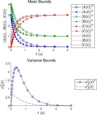
Figure 1: Time-varying bounds on System (53), calculated using $\mathcal{R}=\{0,-2\}$. The points marked with circles and stars each correspond to the solution of an SDP and are theoretically guaranteed bounds. The lines interpolated between these points are not guaranteed bounds. They are included just to lead the eye. The dashed lines are the analytical values, provided by McQuarrie McQuarrie (1967). The top plot shows bounds on the mean molecular count of each species. The bottom plot shows an upper bound on the variance in the molecular count of species A. The other species are omitted, because their variances are identical.

IV.2 Using more values of $\rho$

In Section III.8, we noted that the choice of the set $\mathcal{R}$ can affect the quality of the resulting bounds. We demonstrate this by recalculating the bounds shown in Figure 1 with the enlarged set $\mathcal{R}=\{0,-2,-6\}$. The results are shown in Figure 2. The bounds are noticeably tighter for both the means and the variance, which is consistent with our prior reasoning.

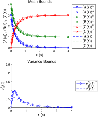
Figure 2: This figure is equivalent to Figure 1 in every way, except that the bounds were calculated using the enlarged set $\mathcal{R}=\{0,-2,-6\}$, giving tighter bounds.

V A Bit More Complexity

In this section, we apply SDPs (44) and (51) to a slightly more complex reaction system, where we’ve added a reversible reaction:

$$\text{A}+\text{B}\autorightarrow{c_{1}}{}\text{C}\autorightleftharpoons{c_{2}}{c_{3}}\text{D}$$ (54)

The rate constants for this system are $c_{1}=1\ \text{s}^{-1},c_{2}=2.1\ \text{s}^{-1},$ and $c_{3}=0.3\ \text{s}^{-1}$ The initial molecular counts of A $=3$, B $=4$, C $=0$, and D $=0$. As with the previous example, this reaction system exhibits the closure problem when subjected to a moment analysis.

V.1 Mean and Variance Bounds

If we repeatedly solve SDP (44) and its minimization counterpart for this system, taking $\mathcal{R}=\{0,-2,-2.4\}$ and $m=3$, we obtain time-varying bounds on the mean molecular counts of each species. Similarly, if we repeatedly solve SDP (51) for this system, with the same $\mathcal{R}$ and $m$, we can obtain time-varying upper bounds on variance for each molecular count. These bounds are shown in the top and bottom panels, respectively, of Figure 3.

In this case, we have no analytical solution. However, the plotted curves match what we would expect. The count of molecules of species B decreases to 1, at which point the molecules of A (not shown in the plot) are exhausted. This is the same behavior we saw in Figures 1 and 2, and this makes sense, because the addition of the reversible reaction in System (54) does not change the dynamics of species A and B. The mean molecular count for species C rises and then falls, leveling off at about 0.5 molecules, while the mean molecular count of species D increases monotonically, leveling off at about 2.5 molecules. The upper bounds on the variances for the two species both approach the same limiting value (about 0.75). This makes sense, because, as the system comes to equilibrium, when no molecules of A and B remain, the probability will be distributed entirely between species C and D, and the uncertainty in the molecular count of one is equal to the uncertainty in the molecular count of the other.

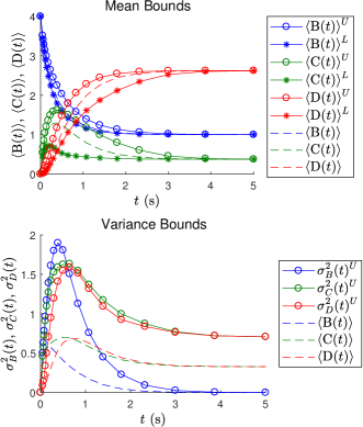
Figure 3: Time-varying bounds on System (54), calculated using $\mathcal{R}=\{0,-2,-2.4\}$. The top plot shows bounds on mean molecular counts, while he bottom plot shows upper bounds on the variances in the counts. Species A is omitted because its behavior closely follows that of species B, and adding extra curves would only clutter the plot. The dashed lines are the true mean and variance trajectories, obtained by direct solution of the CME.

V.2 Using more values of $\rho$

As with the previous example, we now add a value of $\rho$ to our set $\mathcal{R}$, repeat the bounding calculation, and see an improvement in the bounds. In particular, adding $\rho=-4.4$ to our $\mathcal{R}$, we obtain the bounds shown in Figure 4. Comparing with Figure 3, we see substantial improvement in the lower bound of the mean molecular count for species C. We also see that the limiting value of the variance upper bound for species C and D is about half of its previous value. Finally, for each species, the peak in the variance upper bound (around 0.5 s) has been reduced.

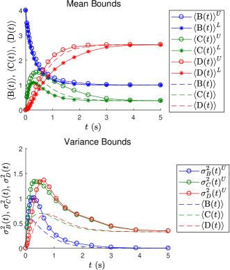
Figure 4: This figure is equivalent to Figure 3 in every way, except that the bounds were calculated using the enlarged set $\mathcal{R}=\{0,-2,-2.4,-4.4\}$, giving better results.

V.3 Sensitivity of the Values of $\rho$

As explained in Section III.5, while any values of $\rho$ will result in theoretically-guaranteed bounds, we recommend picking the values of $\rho$ to match the real parts of the first several distinct eigenvalues of the matrix $\mathbf{G}$, when these eigenvalues are listed in order of increasing magnitude. This is exactly how we chose the values of $\rho$ for the two foregoing examples. These two examples are small enough that we can calculate the eigenvalues directly. However, this will not be the case in general. Usually, the best we can hope for is some numerical approximation of the eigenvalues. This begs the question: how robust is our bounding method to the choice of $\rho$ values? If the values of $\rho$ are off by a little bit, do the bounds become so conservative that they are practically useless?

To explore this idea, we repeated the bounding calculation for Reaction System (54), using a set of perturbed $\rho$ values: $\mathcal{R}=\{0,-1.9,-2.6,-4.7\}$. The resulting bounds are shown in Figure 5. Comparing this plot with Figure 4, we see that the perturbation of the values of $\rho$ did not substantially affect the quality of the computed bounds. We see that the perturbed $\rho$ values create a slight long-time gap in the mean bounds for species C and D, which is undesirable. However, mean bounds on these species at intermediate times (e.g., $t=1$ s) actually seem a little tighter. This demonstrates that the bounding method does not require exact knowledge of the eigenvalues of the underlying CME to obtain reasonable results.

That being said, the choice of $\rho$ values does matter. Using a set of further perturbed $\rho$ values ($\mathcal{R}=\{0,-6,-12,-18\}$), we produced the bounds shown in Figure 6. In this Figure, we see wide gaps in the long-time mean bounds for all species. Furthermore, the variance bounds are much less tight.

In summary, while the chosen values of $\rho$ do not have to match low-magnitude eigenvalues $\mathbf{G}$ exactly, at least approximating them seems to be a good heuristic.

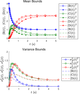
Figure 5: This figure is equivalent to Figure 4, except that the bounds were calculated using the perturbed set $\mathcal{R}=\{0,-1.9,-2.6,-4.7\}$, giving slightly different results. In particular, notice the long-time gap that has appeared in the mean bounds for species C and D.

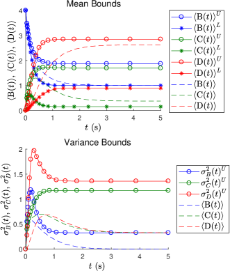
Figure 6: This figure is equivalent to Figures 4 and 5, except that the bounds were calculated using the further perturbed set $\mathcal{R}=\{0,-6,-12,-18\}$. This perturbation dramatically degrades the quality of the bounds.

VI Complex Eigenvalues

Given our observation in Section III.4 that it seems reasonable to choose the values of $\rho$ to match the eigenvalues of the matrix $\mathbf{G}$, it may seem odd that, in Section III.5, we suggested focusing on only the real parts of these eigenvalues. In fact, if we know that some of the low-magnitude eigenvalues have nonzero imaginary parts, we can use this information to obtain tighter bounds.

For example, consider the cyclic system

$$\text{A}+\text{B} \autorightarrow{$c_1$}{}\text{C}$$ (55)

C $$\autorightarrow{$c_2$}{}\text{D}$$

D $$\autorightarrow{$c_3$}{}\text{A}+\text{B}$$

where the initial molecular counts are A $=2$, B $=1$, C $=1$, and D $=0$, and the rate constants are $c_{1}=1\text{ s}^{-1}$, $c_{2}=1.1\text{ s}^{-1}$, and $c_{3}=0.9\text{ s}^{-1}$. The smallest-magnitude eigenvalues of this system are $\lambda=0,-2.1322\pm 0.9741i,-4.1637\pm 1.5837i$. If we follow the advice given in Section III.5, and calculate bounds using $\mathcal{R}=\{0,-2.1322,-4.1637\}$, we obtain the bounds shown in the top panel of Figure 7. However, by making use of the knowledge of the imaginary parts of the eigenvalues, we can produce the slightly improved bounds shown in the bottom panel. The most notable improvements are for early times ($t<0.5\text{ s}$)

Given this potential to improve the bounds by using the imaginary parts of the low-magnitude eigenvalues, why has this paper been concerned almost solely with their real parts? The fact is “making use of the knowledge of the imaginary parts of the eigenvalues” is not trivial. One cannot simply use complex values of $\rho$ in SDPs (44) and (51). The reason for this is that the argument for the derivation of LMIs (39) - (41) breaks down when $\rho$ is complex-valued. It is possible to derive an analogous set of LMIs when $\rho$ is complex-valued, but this requires introducing entirely new classes of decision variables and constraints. The resulting augmented versions of SDPs (44) and (51) are considerably more complicated. We felt that this extra complication would only distract from the main idea of this paper, and, as demonstrated by Figure (7), it leads to only marginal improvement in the bounds. Accordingly, we have deferred the discussion of how to account for complex eigenvalues to the supplementary material.

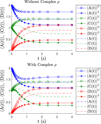
Figure 7: Bounds on the mean molecular counts of species A, C, and D of Reaction System (55). Bounds on species B are omitted, because they are similar to those shown for species A. The top panel shows bounds calculated without accounting for the imaginary components of the system’s eigenvalues, while the bottom panel shows the slight improvement that can be achieved by accounting for these imaginary components. Both panels show the exact means calculated by directly solving the CME.

VII Perfect Bounds in the Absence of the Closure Problem

It is interesting to note that we can also apply our bounding method to stochastic chemical kinetic systems which do not exhibit the closure problem, and that, doing so, it is possible to obtain perfect bounds.

For example, consider the reaction system

$$\text{A}\autorightarrow{c_{1}}{}\text{B}\autorightarrow{c_{2}}{}\text{C},$$ (56)

where $c_{1}=1\text{ s}^{-1}$, $c_{2}=3\text{ s}^{-1}$, and there are initially $4$ molecules of A and $0$ molecules of each B and C. Since every reaction in this system is unimolecular, it does not exhibit the closure problem. The smallest-magnitude eigenvalues for this system are $\lambda=0,-1,-3$. Solving SDP (44) and its minimization counterpart with $\mathcal{R}=\{0,-1,-3\}$, we obtain the bounds shown in Figure 8. The upper and lower bounding curves are indistinguishable from one another because there is essentially no gap between them; they have collapsed upon the true mean trajectories.

This is a rather nice feature of our bounding method, which, frankly, we did not expect. We did not design the method with this collapsing behavior in mind. However, as explained in the supplementary material, it naturally falls out of the math. This example and others like it support the theoretical foundation of our bounding method – in particular, the choice of exponential basis functions.

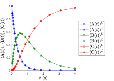
Figure 8: Bounds on the mean molecular counts of species A, B, and C for Reaction System (56), which does not exhibit the closure problem. For this example, the bounding method calculates perfect bounds, collapsing on the true mean trajectories.

VIII Uncertainty in the Initial State

In each of the foregoing examples, we have assumed that we knew the initial molecular count exactly. This implies an initial probability distribution which is a Dirac distribution, where all the probability is concentrated on a single reachable state. However, as suggested in Section (III.2), our method can also handle the more general situation where we don’t have exact knowledge of the initial molecular count, and the initial probability distribution (representing our knowledge of the system) is supported on several reachable states. We demonstrate this capability with the following example.

Again, consider Reaction System (54),

$$\text{A}+\text{B}\autorightarrow{c_{1}}{}\text{C}\autorightleftharpoons{c_{2}}{c_{3}}\text{D},$$

with the same rate constants given in Section V. In our prior analysis of this system, we assumed we knew the initial molecular counts A $=3$, B $=4$, C $=0$, and D $=0$. This implies the set of reachable states $\mathcal{X}$ shown in Table 1.

State	$\mathbf{x}=(x_{\text{A}},x_{\text{B}},x_{\text{C}},x_{\text{D}})$
1	$(3,4,0,0)$
2	$(2,3,1,0)$
3	$(2,3,0,1)$
4	$(1,2,2,0)$
5	$(1,2,1,1)$
6	$(1,2,0,2)$
7	$(0,1,3,0)$
8	$(0,1,2,1)$
9	$(0,1,1,2)$
10	$(0,1,0,3)$

Table 1: The set of reachable states $\mathcal{X}$ of the system described in Section V.

Furthermore, it implies an initial probability of zero for all states in Table 1, except State 1 which has an initial probability of one.

This time, we will assume uncertainty in the initial state, and we will express this uncertainty by assigning a nonzero initial probability to three distinct reachable states $\mathbf{x}\in\mathcal{X}$. In particular, we will assign initial probabilities of $\frac{1}{4},\frac{1}{2}$, and $\frac{1}{4}$ to States 1, 4, and 10, respectively, with all other reachable states having an initial probability of zero. Once we have decided on the set of species to be considered independent (e.g., species A and C), we can easily calculate the initial low-order moments $\bm{\mu}_{L}(0)$ corresponding to this initial distribution $P(\cdot,0)$ using Equation (9). We can then apply SDPs (44) and (51) to calculate bounds on the means and variances for this system over time. For the sake of comparison to Figure 4, we again use $m=3$ and $\mathcal{R}=\{0,-2,-2.4,-4.4\}$. The results are shown in Figure 9.

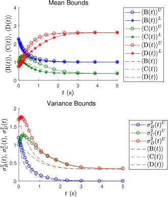
Figure 9: Bounds on the mean and variance for Reaction System (54) with an uncertain initial state.

The first thing to notice in comparing Figures 4 and 9 is that the starting point of each mean and variance trajectory is different between the two figures. This is consistent with the fact that the initial distribution $P(\cdot,0)$ and thus the initial moments $\mathbf{y}_{L}(0)$ are different for the two figures. The second thing to notice is that both plots approach the same steady-state at long times. This is consistent with the fact that Reaction System (54) has just one steady-state, in which species C and D are in equilibrium. Finally, notice that the quality of the bounds is similar between the two plots. At least visually, the bounds in Figure 9 are just as tight as those in Figure 4. This may seem somewhat counter-intuitive given that Figure 9 was generated assuming uncertainty in the initial state. However, recall that once this uncertainty is expressed in an initial probability distribution $P(\cdot,0)$, the means and variances (which are expectation values based on $P(\cdot,0)$) are precisely defined.

IX Conclusion

This paper has described a method for calculating rigorous bounds on time-varying stochastic chemical kinetic systems. In particular, we have formulated SDPs for calculating time-varying bounds on the mean molecular count of each species in the system and the variances in these counts. This idea is an extension of the method described by several authors Dowdy and Barton (2017, 2018); Sakurai and Hori (2017); Kuntz et al. (2017); Ghusinga et al. (2017) for calculating bounds on the steady-state (i.e., stationary) distribution of a stochastic chemical kinetic system.

As a proof of concept, we have demonstrated the bounding method for a simple stochastic chemical system for which analytical means and variances are available. For this example, we have seen that our bounds are, in fact, valid. Furthermore, we have seen that they can be very tight, given the appropriate choice of the parameter set $\mathcal{R}$.

We also applied the bounding method to a slightly more complicated reaction system, which demonstrates that method also applies to systems which reach a dynamic equilibrium at long times. With this example, we saw that the bounds we obtain are not dramatically sensitive to the values of $\rho$ we select in our parameter set $\mathcal{R}$.

While the majority of the paper was written assuming that the parameter set $\mathcal{R}$ contained strictly real values $\rho$, in Section VI we saw that it is possible to obtain improved bounds by also using values of $\rho$ with nonzero imaginary parts – though at the expense of solving a larger, more complicated SDP.

In Section VII, we saw an example which does not exhibit the closure problem, for which the bounds generated by our method collapse upon the true mean trajectories, supporting the theory underlying our approach.

Finally, in Section VIII, we demonstrated that our method can also handle the scenario when the initial state of the system is not known exactly and we instead have nonzero initial probabilities associated with several reachable states.

In theory, our bounding method could be applied to stochastic chemical kinetic systems of arbitrary size. However, to do this, there are two practical issues that must be overcome: first, we need to formalize a procedure for selecting the set $\mathcal{R}$; second, we need to further explore options for mitigating the numerical issues mentioned in Section III.9. Strategies for overcoming these issues will be the subject of a forthcoming publication.

Despite the method’s incompleteness, it is a theoretically novel, interesting approach to the closure problem in stochastic chemical kinetics. We share it with the community in the hope that it might inspire further research in the area.

X Implementation Details

All numerical examples in this paper were computed on a 64-bit Dell Precision T3610 workstation with a 3.70 GHz Intel Xeon CPU. In the example, CVX Grant and Boyd (2014) was used to model the SDP, using the default tolerance (i.e. “precision”) settings. SeDuMi Sturm (1999) was used as the underlying solver.