Adversarially Regularized Graph Autoencoder for Graph Embedding

Abstract

Graph embedding is an effective method to represent graph data in a low dimensional space for graph analytics. Most existing embedding algorithms typically focus on preserving the topological structure or minimizing the reconstruction errors of graph data, but they have mostly ignored the data distribution of the latent codes from the graphs, which often results in inferior embedding in real-world graph data. In this paper, we propose a novel adversarial graph embedding framework for graph data. The framework encodes the topological structure and node content in a graph to a compact representation, on which a decoder is trained to reconstruct the graph structure. Furthermore, the latent representation is enforced to match a prior distribution via an adversarial training scheme. To learn a robust embedding, two variants of adversarial approaches, adversarially regularized graph autoencoder (ARGA) and adversarially regularized variational graph autoencoder (ARVGA), are developed. Experimental studies on real-world graphs validate our design and demonstrate that our algorithms outperform baselines by a wide margin in link prediction, graph clustering, and graph visualization tasks.

1 Introduction

Graphs are essential tools to capture and model complicated relationships among data. In a variety of graph applications, including protein-protein interaction networks, social media, and citation networks, analyzing graph data plays an important role in various data mining tasks including node or graph classification Kipf and Welling (2016a); Pan et al. (2016a), link prediction Wang et al. (2017c), and node clustering Wang et al. (2017a). However, the high computational complexity, low parallelizability, and inapplicability of machine learning methods to graph data have made these graph analytic tasks profoundly challenging Cui et al. (2017). Recently graph embedding has emerged as a general approach to these problems.

Graph embedding converts graph data into a low dimensional, compact, and continuous feature space. The key idea is to preserve the topological structure, vertex content, and other side information Zhang et al. (2017a). This new learning paradigm has shifted the tasks of seeking complex models for classification, clustering, and link prediction to learning a robust representation of the graph data, so that any graph analytic task can be easily performed by employing simple traditional models (e.g., a linear SVM for the classification task). This merit has motivated a number of studies in this area Cai et al. (2017); Goyal and Ferrara (2017).

Graph embedding algorithms can be classified into three categories: probabilistic models, matrix factorization-based algorithms, and deep learning-based algorithms. Probabilistic models like DeepWalk Perozzi et al. (2014), node2vec Grover and Leskovec (2016) and LINE Tang et al. (2015) attempt to learn graph embedding by extracting different patterns from the graph. The captured patterns or walks include global structural equivalence, local neighborhood connectivities, and other various order proximities. Compared with classical methods such as Spectral Clustering Tang and Liu (2011), these graph embedding algorithms perform more effectively and are scalable to large graphs.

Matrix factorization-based algorithms, such as GraRep Cao et al. (2015), HOPE Ou et al. (2016), M-NMF Wang et al. (2017b) pre-process the graph structure into an adjacency matrix and get the embedding by decomposing the adjacency matrix. Recently it has been shown that many probabilistic algorithms are equivalent to matrix factorization approaches Qiu et al. (2017). Deep learning approaches, especially autoencoder-based methods, are also widely studied for graph embedding. SDNE Wang et al. (2016) and DNGR Cao et al. (2016) employ deep autoencoders to preserve the graph proximities and model positive pointwise mutual information (PPMI). The MGAE algorithm utilizes a marginalized single layer autoencoder to learn representation for clustering Wang et al. (2017a).

The approaches above are typically unregularized approaches which mainly focus on preserving the structure relationship (probabilistic approaches), or minimizing the reconstruction error (matrix factorization or deep learning methods). They have mostly ignored the data distribution of the latent codes. In practice unregularized embedding approaches often learn a degenerate identity mapping where the latent code space is free of any structure Makhzani et al. (2015), and can easily result in poor representation in dealing with real-world sparse and noisy graph data. One common way to handle this problem is to introduce some regularization to the latent codes and enforce them to follow some prior data distribution Makhzani et al. (2015). Recently generative adversarial based frameworks Donahue et al. (2016); Radford et al. (2015) have also been developed for learning robust latent representation. However, none of these frameworks is specifically for graph data, where both topological structure and content information are required to embed to a latent space.

In this paper, we propose a novel adversarial framework with two variants, namely adversarially regularized graph autoencoder (ARGA) and adversarially regularized variational graph autoencoder (ARVGA), for graph embedding. The theme of our framework is to not only minimize the reconstruction errors of the graph structure but also to enforce the latent codes to match a prior distribution. By exploiting both graph structure and node content with a graph convolutional network, our algorithms encodes the graph data in the latent space. With a decoder aiming at reconstructing the topological graph information, we further incorporate an adversarial training scheme to regularize the latent codes to learn a robust graph representation. The adversarial training module aims to discriminate if the latent codes are from a real prior distribution or from the graph encoder. The graph encoder learning and adversarial regularization are jointly optimized in a unified framework so that each can be beneficial to the other and finally lead to a better graph embedding. The experimental results on benchmark datasets demonstrate the superb performance of our algorithms on three unsupervised graph analytic tasks, namely link prediction, node clustering, and graph visualization. Our contributions can be summarized below:

• We propose a novel adversarially regularized framework for graph embedding, which represent topological structure and node content in a continuous vector space. Our framework learns the embedding to minimize the reconstruction error while enforcing the latent codes to match a prior distribution.

• We develop two variants of adversarial approaches, adversarially regularized graph autoencoder (ARGA) and adversarially regularized variational graph autoencoder (ARVGA) to learn the graph embedding.

• Experiments on benchmark graph datasets demonstrate that our graph embedding approaches outperform the others on three unsupervised tasks.

2 Related Work

Graph Embedding Models. From the perspective of information exploration, graph embedding algorithms can be also separated into two groups: topological embedding approaches and content enhanced embedding methods.

Topological embedding approaches assume that there is only topological structure information available, and the learning objective is to preserve the topological information maximumly. Perozzi et al. propose a DeepWalk model to learn the node embedding from a collection of random walks Perozzi et al. (2014). Since then, a number of probabilistic models such as node2vec Grover and Leskovec (2016) and LINE Tang et al. (2015) have been developed. As a graph can be mathematically represented as an adjacency matrix, many matrix factorization approaches such as GraRep Cao et al. (2015), HOPE Ou et al. (2016), M-NMF Wang et al. (2017b) are proposed to learn the latent representation for a graph. Recently deep learning models have been widely exploited to learn the graph embedding. These algorithms preserve the first and second order of proximities Wang et al. (2016), or reconstruct the positive pointwise mutual information (PPMI) Cao et al. (2016) via different variants of autoencoders.

Content enhanced embedding methods assume node content information is available and exploit both topological information and content features simultaneously. TADW Yang et al. (2015) presents a matrix factorization approach to explore node features. TriDNR Pan et al. (2016b) captures structure, node content, and label information via a tri-party neural network architecture. UPP-SNE employs an approximated kernel mapping scheme to exploit user profile features to enhance the embedding learning of users in social networks Zhang et al. (2017b).

Unfortunately the above algorithms largely ignore the latent distribution of the embedding, which may result in poor representation in practice. In this paper, we explore adversarial training methods to address this issue.

Adversarial Models. Our method is motivated by the generative adversarial network (GAN) Goodfellow et al. (2014). GAN plays an adversarial game with two linked models: the generator $\mathcal{G}$ and the discriminator $\mathcal{D}$. The discriminator can be a multi-layer perceptron which discriminates if an input sample comes from the data distribution or from the generator we built. Simultaneously, the generator is trained to generate the samples to convince the discriminator that the generated samples come from the prior data distribution. Due to its effectiveness in many unsupervised tasks, recently a number of adversarial training algorithms have been proposed Donahue et al. (2016); Radford et al. (2015).

Recently Makhzani et al. proposed an adversarial autoencoder (AAE) to learn the latent embedding by merging the adversarial mechanism into the autoencoder Makhzani et al. (2015). However, it is designed for general data rather than graph data. Dai et al. applied the adversarial mechanism to graphs. However, their approach can only exploit the topological information Dai et al. (2017). In contrast, our algorithm is more flexible and can handle both topological and content information for graph data.

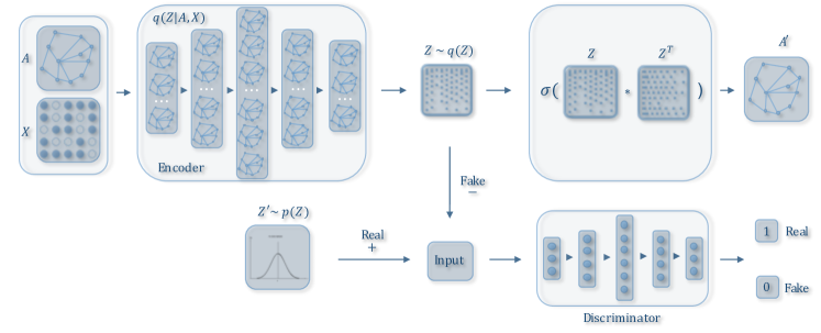
Figure 1: The architecture of the adversarially regularized graph autoencoder (ARGA). The upper tier is a graph convolutional autoencoder that reconstructs a graph $\mathbf{A}$ from an embedding $\mathbf{Z}$ which is generated by the encoder which exploits graph structure $\mathbf{A}$ and the node content matrix $\mathbf{X}$. The lower tier is an adversarial network trained to discriminate if a sample is generated from the embedding or from a prior distribution. The adversarially regularized variational graph autoencoder (ARVGA) is similar to ARGA except that it employs a variational graph autoencoder in the upper tier (See Algorithm 1 for details).

3 Problem Definition and Framework

A graph is represented as $\mathbf{G}=\{\mathbf{V},\mathbf{E},\mathbf{X}\}$, where $\mathbf{V}=\{\mathbf{v}_{i}\}_{i}=1,\cdots,n$ consists of a set of nodes in a graph and $\mathbf{e}_{i,j}=<\mathbf{v}_{i},\mathbf{v}_{j}>\in\mathbf{E}$ represents a linkage encoding the citation edge between the nodes. The topological structure of graph $\mathbf{G}$ can be represented by an adjacency matrix $\mathbf{A}$, where $\mathbf{A}_{i,j}=1$ if $\mathbf{e}_{i,j}\in\mathbf{E}$, otherwise $\mathbf{A}_{i,j}=0$. $\mathbf{x}_{i}\in\mathbf{X}$ indicates the content features associated with each node $\mathbf{v}_{i}$.

Given a graph $\mathbf{G}$, our purpose is to map the nodes $\mathbf{v}_{i}\in\mathbf{V}$ to low-dimensional vectors $\mathbf{z}_{i}\in\mathbb{R}^{d}$ with the formal format as follows: $f:\mathbf{(A,X)}\rightarrowtail\mathbf{Z}$, where $\mathbf{z}_{i}^{\top}$ is the $i$-th row of the matrix $\mathbf{Z}\in\mathbb{R}^{n\times d}$. $n$ is the number of nodes and $d$ is the dimension of embedding. We take $\mathbf{Z}$ as the embedding matrix and the embeddings should well preserve the topological structure $\mathbf{A}$ as well as content information $\mathbf{X}$ .

3.1 Overall Framework

Our objective is to learn a robust embedding given a graph $\mathbf{G}=\{\mathbf{V},\mathbf{E},\mathbf{X}\}$. To this end, we leverage an adversarial architecture with a graph autoencoder to directly process the entire graph and learn a robust embedding. Figure 1 demonstrates the workflow of ARGA which consists of two modules: the graph autoencoder and the adversarial network.

• Graph Convolutional Autoencoder. The autoencoder takes in the structure of graph $\mathbf{A}$ and the node content $\mathbf{X}$ as inputs to learn a latent representation $\mathbf{Z}$, and then reconstructs the graph structure $\mathbf{A}$ from $\mathbf{Z}$.

• Adversarial Regularization. The adversarial network forces the latent codes to match a prior distribution by an adversarial training module, which discriminates whether the current latent code $\mathbf{z}_{i}\in\mathbf{Z}$ comes from the encoder or from the prior distribution.

4 Proposed Algorithm

4.1 Graph Convolutional Autoencoder

The graph convolutional autoencoder aims to embed a graph $\mathbf{G}=\{\mathbf{V},\mathbf{E},\mathbf{X}\}$ in a low-dimensional space. Two key questions arise (1) how to integrate both graph structure $\mathbf{A}$ and node content $\mathbf{X}$ in an encoder, and (2) what sort of information should be reconstructed via a decoder?

Graph Convolutional Encoder Model $\mathcal{G}(\mathbf{X},\mathbf{A})$.   To represent both graph structure $\mathbf{A}$ and node content $\mathbf{X}$ in a unified framework, we develop a variant of the graph convolutional network (GCN) Kipf and Welling (2016a) as a graph encoder. Our graph convolutional network (GCN) extends the operation of convolution to graph data in the spectral domain, and learns a layer-wise transformation by a spectral convolution function $f(\mathbf{Z}^{(l)},\mathbf{A}|\mathbf{W}^{(l)})$:

$$\mathbf{Z}^{(l+1)}=f(\mathbf{Z}^{(l)},\mathbf{A}|\mathbf{W}^{(l)})$$ (1)

Here, $\mathbf{Z}^{l}$ is the input for convolution, and $\mathbf{Z}^{(l+1)}$ is the output after convolution. We have $\mathbf{Z}^{0}=\mathbf{X}\in\mathbb{R}^{n\times m}$ ($n$ nodes and $m$ features) for our problem. $\mathbf{W}^{(l)}$ is a matrix of filter parameters we need to learn in the neural network. If $f(\mathbf{Z}^{(l)},\mathbf{A}|\mathbf{W}^{(l)})$ is well defined, we can build arbitrary deep convolutional neural networks efficiently.

Each layer of our graph convolutional network can be expressed with the function $f(\mathbf{Z}^{(l)},\mathbf{A}|\mathbf{W}^{(l)})$ as follows:

$$f(\mathbf{Z}^{(l)},\mathbf{A}|\mathbf{W}^{(l)})=\phi(\widetilde{\mathbf{D}}^{-\frac{1}{2}}\widetilde{\mathbf{A}}\widetilde{\mathbf{D}}^{-\frac{1}{2}}\mathbf{Z}^{(l)}\mathbf{W}^{(l)}),$$ (2)

where $\widetilde{\mathbf{A}}=\mathbf{A}+\mathbf{I}$ and $\widetilde{\mathbf{D}}_{ii}=\sum_{j}\widetilde{\mathbf{A}}_{ij}$. $\mathbf{I}$ is the identity matrix of ${\mathbf{A}}$ and $\phi$ is an activation function such as $\text{Relu}(t)=\max(0,t)$ or $\text{sigmoid}(t)=\frac{1}{1+e^{t}}$. Overall, the graph encoder $\mathcal{G}(\mathbf{X},\mathbf{A})$ is constructed with a two-layer GCN. In our paper, we develop two variants of encoder, e.g., Graph Encoder and Variational Graph Encoder.

The Graph Encoder is constructed as follows:

$$\mathbf{Z}^{(1)}=f_{\text{Relu}}(\mathbf{X},\mathbf{A}|\mathbf{W}^{(0)});$$ (3)

$$\mathbf{Z}^{(2)}=f_{\text{linear}}(\mathbf{Z}^{(1)},\mathbf{A}|\mathbf{W}^{(1)}).$$ (4)

$\text{Relu}(\cdot)$ and linear activation functions are used for the first and second layers. Our graph convolutional encoder $\mathcal{G}(\mathbf{Z},\mathbf{A})=q(\mathbf{Z}|\mathbf{X},\mathbf{A})$ encodes both graph structure and node content into a representation $\mathbf{Z}=q(\mathbf{Z}|\mathbf{X},\mathbf{A})=\mathbf{Z}^{(2)}$.

A Variational Graph Encoder is defined by an inference model:

$$q(\mathbf{Z}|\mathbf{X},\mathbf{A})=\prod^{n}_{i=1}q(\mathbf{z_{i}}|\mathbf{X},\mathbf{A}),$$ (5)

$$q(\mathbf{z_{i}}|\mathbf{X},\mathbf{A})=\mathcal{N}(\mathbf{z}_{i}|\bm{{\mu}}_{i},\text{diag}(\bm{\sigma}^{2}))$$ (6)

Here, $\bm{\mu}=\mathbf{Z}^{(2)}$ is the matrix of mean vectors $\bm{z}_{i}$ ; similarly $\text{log}\bm{\sigma}=f_{\text{linear}}(\mathbf{Z}^{(1)},\mathbf{A}|\mathbf{W}^{\prime(1)})$ which share the weights $\mathbf{W}^{(0)}$ with $\bm{\mu}$ in the first layer in Eq. (3).

Decoder Model.   Our decoder model is used to reconstruct the graph data. We can reconstruct either the graph structure $\mathbf{A}$, content information $\mathbf{X}$, or both. In our paper, we propose to reconstruct graph structure $\mathbf{A}$, which provides more flexibility in the sense that our algorithm will still function properly even if there is no content information $\mathbf{X}$ available (e.g., $\mathbf{X}=\mathbf{I}$). Our decoder $p(\hat{\mathbf{A}}|\mathbf{Z})$ predicts whether there is a link between two nodes. More specifically, we train a link prediction layer based on the graph embedding:

$$\small p(\hat{\mathbf{A}}|\mathbf{Z})=\prod^{n}_{i=1}\prod^{n}_{j=1}p(\hat{\mathbf{A}}_{ij}|\mathbf{z}_{i},\mathbf{z}_{j});$$ (7)

$$p(\hat{\mathbf{A}}_{ij}=1|\mathbf{z}_{i},\mathbf{z}_{j})=\text{sigmoid}(\mathbf{z}^{\top}_{i},\mathbf{z}_{j}),$$ (8)

Graph Autoencoder Model.   The embedding $\mathbf{Z}$ and the reconstructed graph $\hat{\mathbf{A}}$ can be presented as follows:

$$\hat{\mathbf{A}}=\text{sigmoid}(\mathbf{Z}\mathbf{Z}^{\top}),\ \text{here}\ \mathbf{Z}=q(\mathbf{Z}|\mathbf{X},\mathbf{A})$$ (9)

Optimization.   For the graph encoder, we minimize the reconstruction error of the graph data by:

$$\mathcal{L}_{0}=\mathbb{E}_{q(\mathbf{Z|(X,A)})}[\text{log}~{}p(\hat{\mathbf{A}}|\mathbf{Z})]$$ (10)

For the variational graph encoder, we optimize the variational lower bound as follows:

$$\mathcal{L}_{1}=\mathbb{E}_{q(\mathbf{Z|(X,A)})}[\text{log}~{}p(\hat{\mathbf{A}}|\mathbf{Z})]-\mathbf{KL}[q(\mathbf{Z|\mathbf{X}},\mathbf{A})\parallel p(\mathbf{Z})]$$ (11)

where $\mathbf{KL}[q(\bullet)||p(\bullet)]$ is the Kullback-Leibler divergence between $q(\bullet)$ and $p(\bullet)$. We also take a Gaussian prior $p(\mathbf{Z})=\prod_{i}p(\mathbf{z}_{i})=\prod_{i}\mathcal{N}(\mathbf{z}_{i}|0,\mathbf{I})$.

4.2 Adversarial Model $\mathcal{D}(\mathbf{Z})$

The key idea of our model is to enforce latent representation $\mathbf{Z}$ to match a prior distribution, which is achieved by an adversarial training model. The adversarial model is built on a standard multi-layer perceptron (MLP) where the output layer only has one dimension with a sigmoid function. The adversarial model acts as a discriminator to distinguish whether a latent code is from the prior $p_{z}$ (positive) or from graph encoder $\mathcal{G}(\mathbf{X,A})$ (negative). By minimizing the cross-entropy cost for training the binary classifier, the embedding will finally be regularized and improved during the training process. The cost can be computed as follows:

$$-\frac{1}{2}\mathbb{E}_{\mathbf{z}\sim p_{z}}\text{log}\mathcal{D}(\mathbf{Z})-\frac{1}{2}\mathbb{E}_{\mathbf{X}}\text{log}(1-\mathcal{D}(\mathcal{G}(\mathbf{X,A}))),$$ (12)

In our paper, we use simple Gaussian distribution as $p_{z}$.

Adversarial Graph Autoencoder Model.   The equation for training the encoder model with Discriminator $\mathcal{D(\mathbf{Z})}$ can be written as follows:

$$\small\min_{\mathcal{G}}\max_{\mathcal{D}}\mathbb{E}_{\mathbf{z}\sim p_{z}}[\text{log}\mathcal{D(\mathbf{Z})}]+\mathbb{E}_{\mathbf{x}\sim p(\mathbf{x})}[\text{log}(1-\mathcal{D}(\mathcal{G}(\mathbf{X,A})))]$$ (13)

where $\mathcal{G}(\mathbf{X,A})$ and $\mathcal{D(\mathbf{Z})}$ indicate the generator and discriminator explained above.

Algorithm 1 Adversarially Regularized Graph Embedding

0:  $\mathbf{G}=\{\mathbf{V},\mathbf{E},\mathbf{X}\}$: a Graph with links and features;$T$: the number of iterations;$K$: the number of steps for iterating discriminator;$d$: the dimension of the latent variable

0:  $\mathbf{Z}\in\mathbb{R}^{n\times d}$

1:  for iterator = 1,2,3, $\cdots\cdots$, $T$ do

2:     Generate latent variables matrix $\mathbf{Z}$ through Eq.(4);

3:     for k = 1,2, $\cdots\cdots$, $K$ do

4:        Sample $m$ entities {$\mathbf{z}^{(1)}$, …, $\mathbf{z}^{(m)}$} from latent matrix $\mathbf{Z}$

5:        Sample $m$ entities {$\mathbf{a}^{(1)}$, …, $\mathbf{a}^{(m)}$} from the prior distribution $p_{z}$

6:        Update the discriminator with its stochastic gradient:

$$\bigtriangledown\frac{1}{m}\sum^{m}_{i=1}[\text{log~{}}\mathcal{D}(\mathbf{a}^{i})+\text{log~{}}(1-\mathcal{D}(\mathbf{z}^{(i)}))]$$

$\mathbf{end}\ \mathbf{for}$

7:     Update the graph autoencoder with its stochastic gradient by Eq. (10) for ARGA or Eq. (11) for ARVGA; $\mathbf{end}\ \mathbf{for}$

8:  return  $\mathbf{Z}\in\mathbb{R}^{n\times d}$

4.3 Algorithm Explanation

Algorithm 1 is our proposed framework. Given a graph $\mathbf{G}$, the step 2 gets the latent variables matrix $\mathbf{Z}$ from the graph convolutional encoder. Then we take the same number of samples from the generated $\mathbf{Z}$ and the real data distribution $p_{z}$ in step 4 and 5 respectively, to update the discriminator with the cross-entropy cost computed in step 6. After $K$ runs of training the discriminator, the graph encoder will try to confuse the trained discriminator and update itself with generated gradient in step 7. We can update Eq. (10) to train the adversarially regularized graph autoencoder (ARGA), or Eq. (11) to train the adversarially regularized variational graph autoencoder (ARVGA), respectively. Finally, we will return the graph embedding $\mathbf{Z}\in\mathbb{R}^{n\times d}$ in step 8.

5 Experiments

We report our results on three unsupervised graph analytic tasks: link prediction, node clustering, and graph visualization. The benchmark graph datasets used in the paper are summarized in Table 1. Each data set consists of scientific publications as nodes and citation relationships as edges. The features are unique words in each document.

Data Set	# Nodes	# Links	# Content Words	# Features
Cora	2,708	5,429	3,880,564	1,433
Citeseer	3,327	4,732	12,274,336	3,703
PubMed	19,717	44,338	9,858,500	500

Table 1: Real-world Graph Datasets Used in the Paper

5.1 Link Prediction

Baselines.   We compared our algorithms against state-of-the-art algorithms for the link prediction task:

• DeepWalk Perozzi et al. (2014): is a network representation approach which encodes social relations into a continuous vector space.

• Spectral Clustering Tang and Liu (2011): is an effective approach for learning social embedding.

• GAE Kipf and Welling (2016b): is the most recent autoencoder-based unsupervised framework for graph data, which naturally leverages both topological and content information.

• VGAE Kipf and Welling (2016b): is a variational graph autoencoder approach for graph embedding with both topological and content information.

• ARGA: Our proposed adversarially regularized autoencoder algorithm which uses graph autoencoder to learn the embedding.

• ARVGA: Our proposed algorithm, which uses a variational graph autoencoder to learn the embedding.

Metrics.   We report the results in terms of AUC score (the area under a receiver operating characteristic curve) and average precision (AP) Kipf and Welling (2016b) score. We conduct each experiment 10 times and report the mean values with the standard errors as the final scores. Each dataset is separated into a training, testing set and validation set. The validation set contains 5% citation edges for hyperparameter optimization, the test set holds 10% citation edges to verify the performance, and the rest are used for training.

Parameter Settings. For the Cora and Citeseer data sets, we train all autoencoder-related models for 200 iterations and optimize them with the Adam algorithm. Both learning rate and discriminator learning rate are set as 0.001. As the PubMed data set is relatively large (around 20,000 nodes), we iterate 2,000 times for an adequate training with a 0.008 discriminator learning rate and 0.001 learning rate. We construct encoders with a 32-neuron hidden layer and a 16-neuron embedding layer for all the experiments and all the discriminators are built with two hidden layers(16-neuron, 64-neuron respectively). For the rest of the baselines, we retain to the settings described in the corresponding papers.

Experimental Results.   The details of the experimental results on the link prediction are shown in Table 2. The results show that by incorporating an effective adversarial training module into our graph convolutional autoencoder, ARGA and ARVGA achieve outstanding performance: all AP and AUC scores are as higher as 92% on all three data sets. Compared with all the baselines, ARGE increased the AP score from around 2.5% compared with VGAE incorporating with node features, 11% compared with VGAE without node features; 15.5% and 10.6% compared with DeepWalk and Spectral Clustering respectively on the large PubMed data set .

Parameter Study.   We vary the dimension of embedding from 8 neurons to 1024 and report the results in Fig 2.

The results from both Fig 2 (A) and (B) reveal similar trends: when adding the dimension of embedding from 8-neuron to 16-neuron, the performance of embedding on link prediction steadily rises; but when we further increase the number of the neurons at the embedding layer to 32-neuron, the performance fluctuates however the results for both the AP score and the AUC score remain good.

It is worth mentioning that if we continue to set more neurons, for examples, 64-neuron, 128-neuron and 1024-neuron, the performance rises markedly.

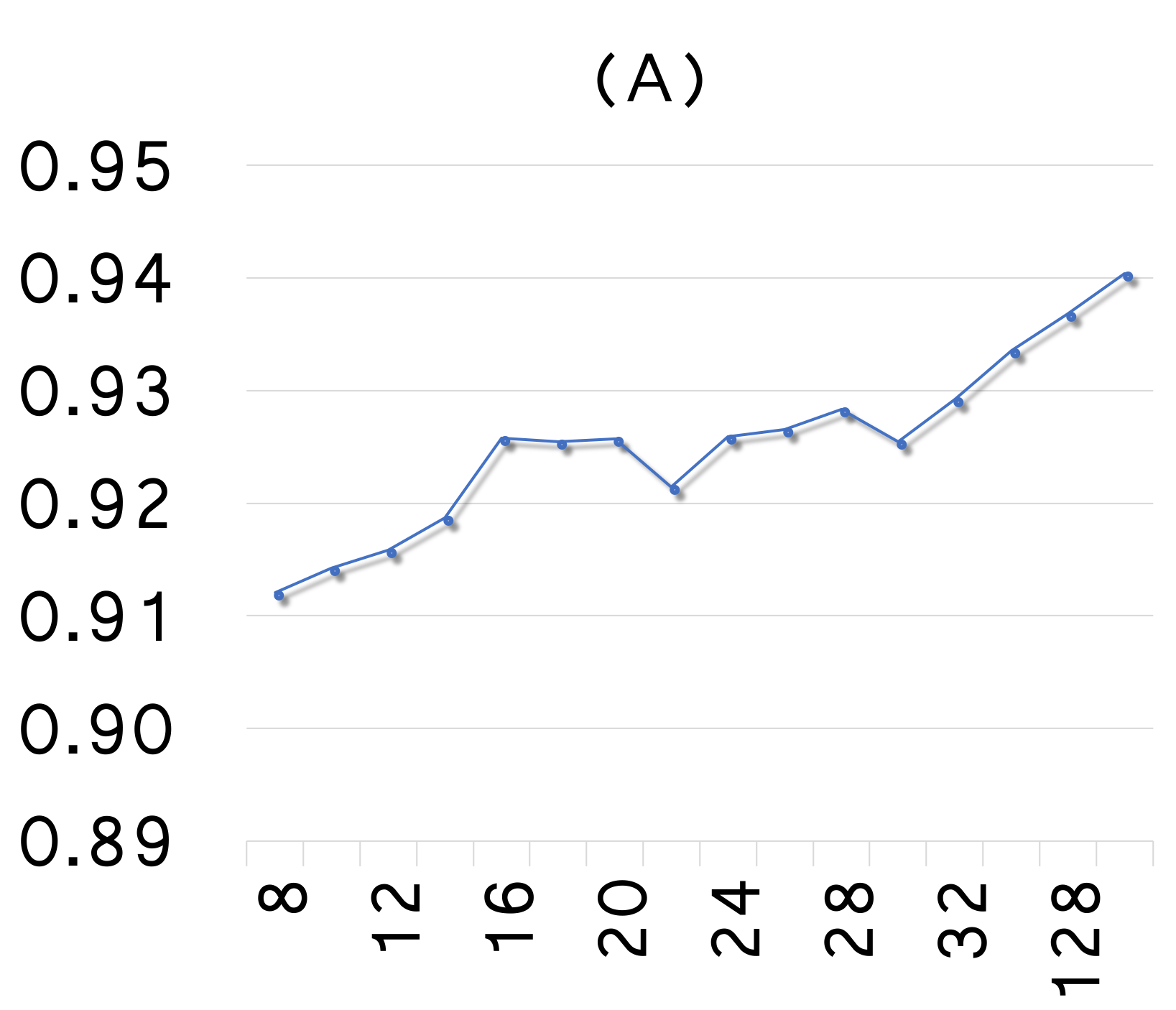
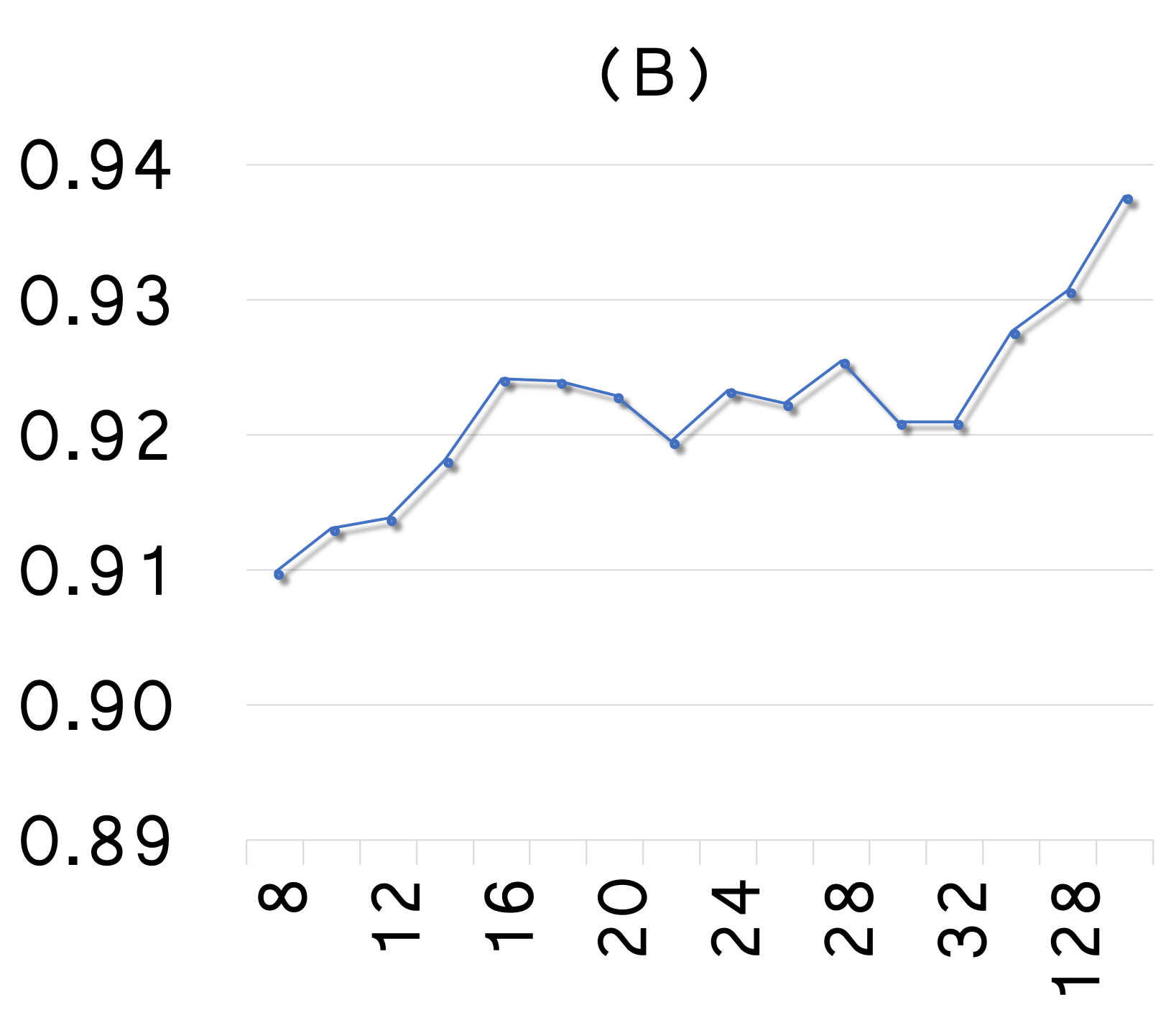
Figure 2: Average performance on different dimensions of the embedding. (A) Average Precision score; (B) AUC score.

Approaches	Cora		Citeseer		PubMed
	AUC	AP	AUC	AP	AUC	AP
SC	84.6 $\pm$ 0.01	88.5 $\pm$ 0.00	80.5 $\pm$ 0.01	85.0 $\pm$ 0.01	84.2 $\pm$ 0.02	87.8 $\pm$ 0.01
DW	83.1 $\pm$ 0.01	85.0 $\pm$ 0.00	80.5 $\pm$ 0.02	83.6 $\pm$ 0.01	84.4 $\pm$ 0.00	84.1 $\pm$ 0.00
$\text{GAE}^{*}$	84.3 $\pm$ 0.02	88.1 $\pm$ 0.01	78.7 $\pm$ 0.02	84.1 $\pm$ 0.02	82.2 $\pm$ 0.01	87.4 $\pm$ 0.00
$\text{VGAE}^{*}$	84.0 $\pm$ 0.02	87.7 $\pm$ 0.01	78.9 $\pm$ 0.03	84.1 $\pm$ 0.02	82.7 $\pm$ 0.01	87.5 $\pm$ 0.01
GAE	91.0 $\pm$ 0.02	92.0 $\pm$ 0.03	89.5 $\pm$ 0.04	89.9 $\pm$ 0.05	96.4 $\pm$ 0.00	96.5 $\pm$ 0.00
VGAE	91.4 $\pm$ 0.01	92.6 $\pm$ 0.01	90.8 $\pm$ 0.02	92.0 $\pm$ 0.02	94.4 $\pm$ 0.02	94.7 $\pm$ 0.02
ARGE	92.4 $\pm$ 0.003	93.2 $\pm$ 0.003	91.9 $\pm$ 0.003	93.0$\pm$ 0.003	96.8 $\pm$ 0.001	97.1 $\pm$ 0.001
ARVGE	92.4 $\pm$ 0.004	92.6 $\pm$ 0.004	92.4 $\pm$ 0.003	93.0 $\pm$ 0.003	96.5$\pm$ 0.001	96.8$\pm$ 0.001

Table 2: Results for Link Prediction. $\text{GAE}^{*}$ and $\text{VGAE}^{*}$ are variants of GAE, which only explore topological structure, i.e., $\mathbf{X}=\mathbf{I}$.

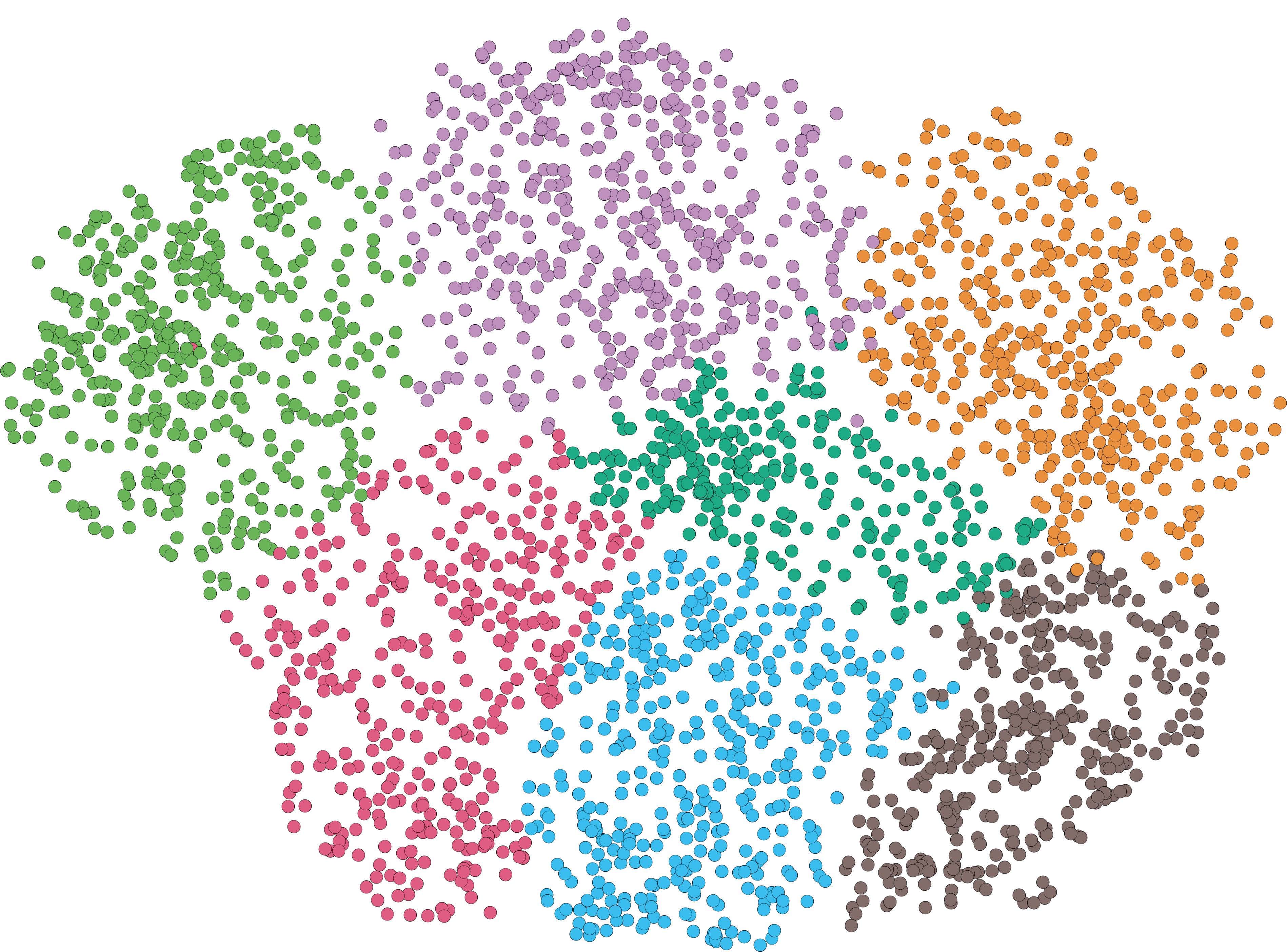
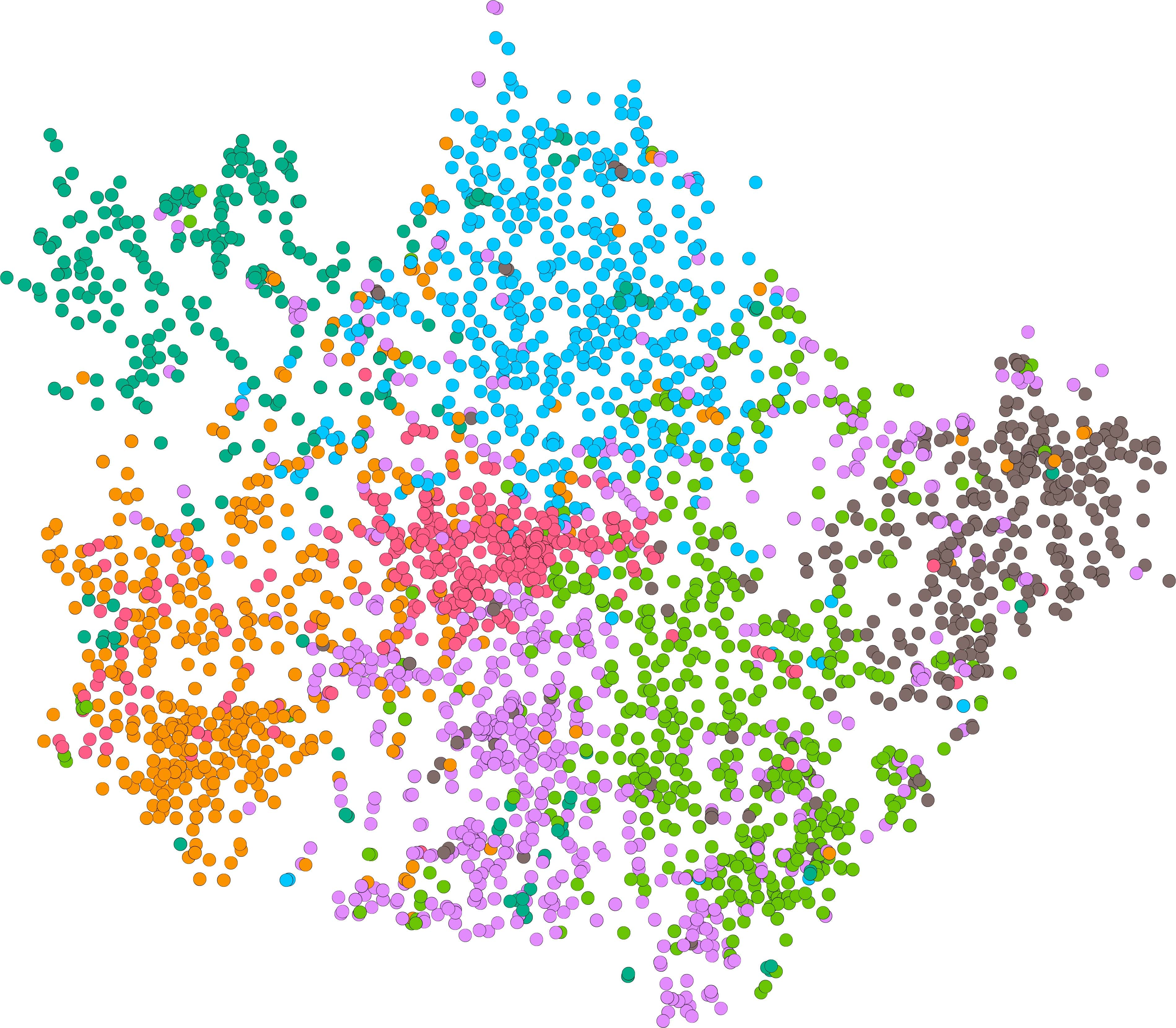
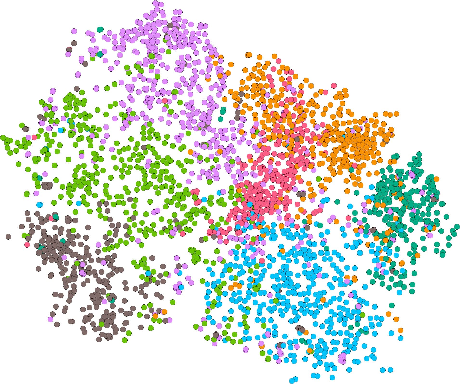
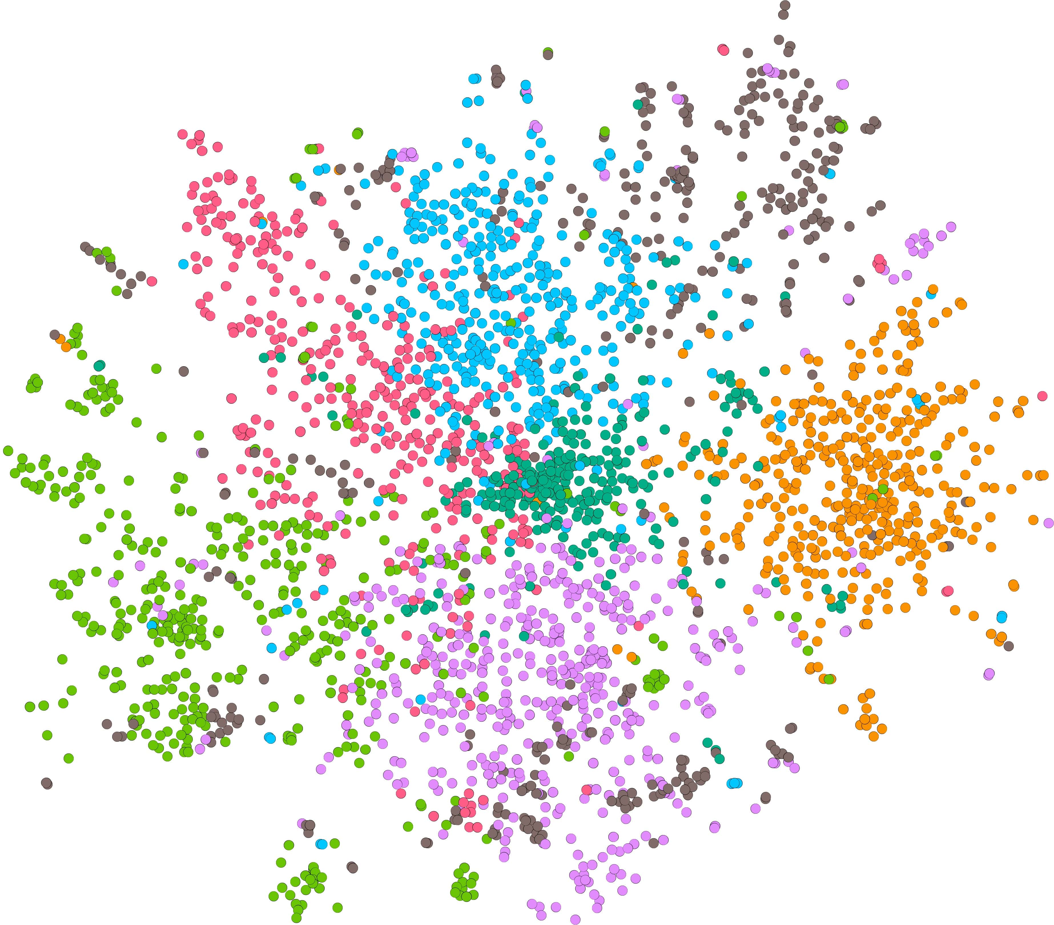
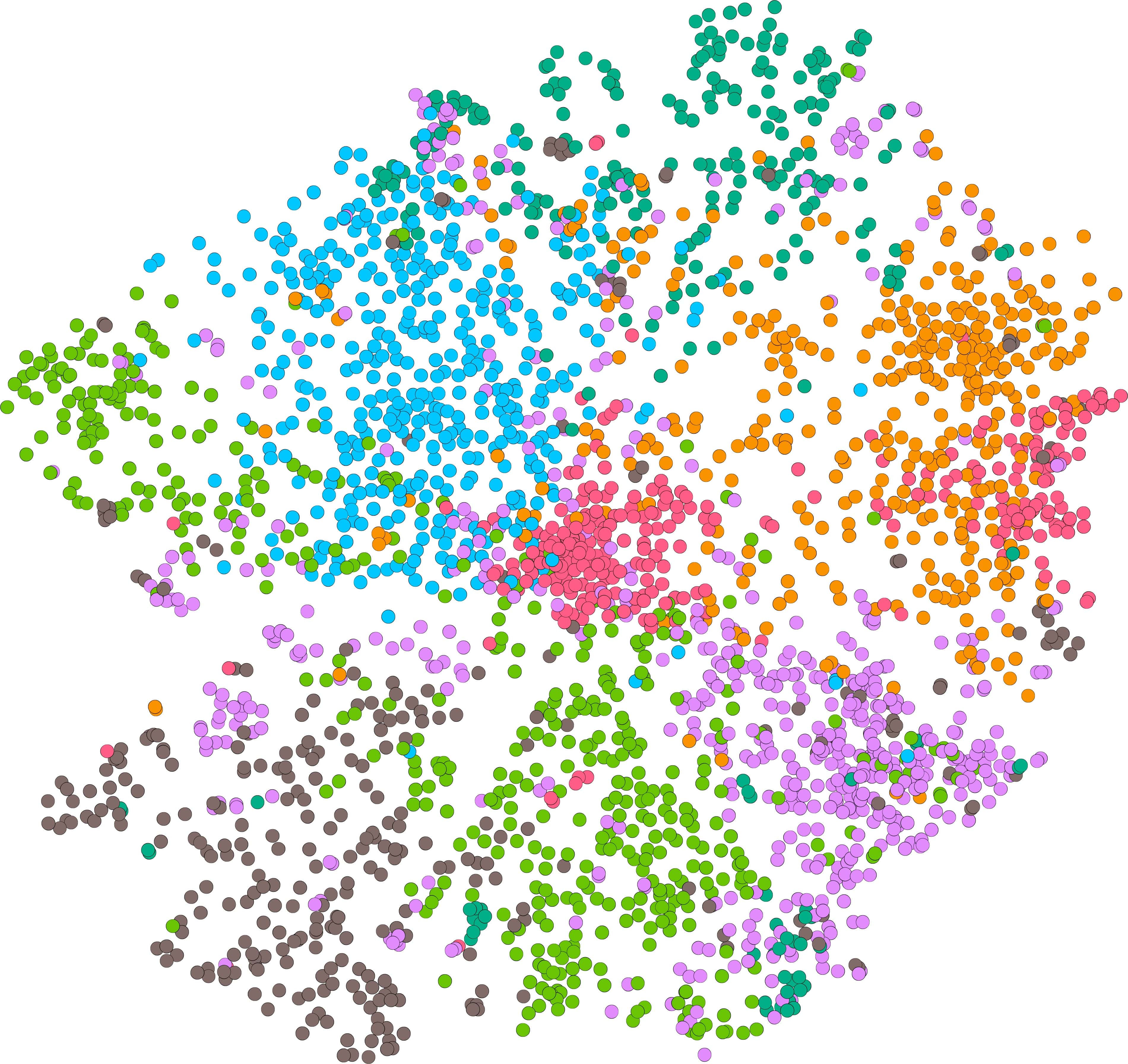
Figure 3: The Cora data visualization comparison. From left to right: embeddings from our ARGA, VGAE, GAE, DeepWalk, and Spectral Clustering. The different colors represent different groups.

5.2 Node Clustering

For the node clustering task, we first learn the graph embedding, and then perform K-means clustering algorithm based on the embedding.

Baselines. We compare both embedding based approaches as well as approaches directly for graph clustering. Except for the baselines we compared for link prediction, we also include baselines which are designed for clustering:

1. K-means is a classical method and also the foundation of many clustering algorithms.

2. Graph Encoder Tian et al. (2014) learns graph embedding for spectral graph clustering.

3. DNGR Cao et al. (2016) trains a stacked denoising autoencoder for graph embedding.

4. RTM Chang and Blei (2009) learns the topic distributions of each document from both text and citation.

5. RMSC Xia et al. (2014) employs a multi-view learning approach for graph clustering.

6. TADW Yang et al. (2015) applies matrix factorization for network representation learning.

Here the first three algorithms only exploit the graph structures, while the last three algorithms use both graph structure and node content for the graph clustering task.

Metrics.   Following Xia et al. (2014), we employ five metrics to validate the clustering results: accuracy (Acc), normalized mutual information (NMI), precision, F-score (F1) and average rand index (ARI).

Experimental Results.   The clustering results on the Cora and Citeseer data sets are given in Table 3 and Table 4. The results show that ARGA and ARVGA have achieved a dramatic improvement on all five metrics compared with all the other baselines. For instance, on Citeseer, ARGA has increased the accuracy from 6.1% compared with K-means to 154.7% compared with GraphEncoder; increased the F1 score from 31.9% compared with TADW to 102.2% compared with DeepWalk; and increased NMI from 14.8% compared with K-means to 124.4% compared with VGAE. The wide margin in the results between ARGE and GAE (and the others) has further proved the superiority of our adversarially regularized graph autoencoder.

Cora	Acc	NMI	F1	Precision	ARI
K-means	0.492	0.321	0.368	0.369	0.230
Spectral	0.367	0.127	0.318	0.193	0.031
GraphEncoder	0.325	0.109	0.298	0.182	0.006
DeepWalk	0.484	0.327	0.392	0.361	0.243
DNGR	0.419	0.318	0.340	0.266	0.142
RTM	0.440	0.230	0.307	0.332	0.169
RMSC	0.407	0.255	0.331	0.227	0.090
TADW	0.560	0.441	0.481	0.396	0.332
GAE	0.596	0.429	0.595	0.596	0.347
VGAE	0.609	0.436	0.609	0.609	0.346
ARGE	0.640	0.449	0.619	0.646	0.352
ARVGE	0.638	0.450	0.627	0.624	0.374

Table 3: Clustering Results on Cora

5.3 Graph Visualization

We visualize the Cora data in a two-dimensional space by applying the t-SNE algorithm Maaten (2014) on the learned embedding. The results in Fig 3 validate that by applying adversarial training to the graph data, we can obtained a more meaningful layout of the graph data.

Citeseer	Acc	NMI	F1	Precision	ARI
K-means	0.540	0.305	0.409	0.405	0.279
Spectral	0.239	0.056	0.299	0.179	0.010
GraphEncoder	0.225	0.033	0.301	0.179	0.010
DeepWalk	0.337	0.088	0.270	0.248	0.092
DNGR	0.326	0.180	0.300	0.200	0.044
RTM	0.451	0.239	0.342	0.349	0.203
RMSC	0.295	0.139	0.320	0.204	0.049
TADW	0.455	0.291	0.414	0.312	0.228
GAE	0.408	0.176	0.372	0.418	0.124
VGAE	0.344	0.156	0.308	0.349	0.093
ARGE	0.573	0.350	0.546	0.573	0.341
ARVGE	0.544	0.261	0.529	0.549	0.245

Table 4: Clustering Results on Citeseer

6 Conclusion

In this paper, we proposed a novel adversarial graph embedding framework for graph data. We argue that most existing graph embedding algorithms are unregularized methods that ignore the data distributions of the latent representation and suffer from inferior embedding in real-world graph data. We proposed an adversarial training scheme to regularize the latent codes and enforce the latent codes to match a prior distribution. The adversarial module is jointly learned with a graph convolutional autoencoder to produce a robust representation. Experiment results demonstrated that our algorithms ARGA and ARVGA outperform baselines in link prediction, node clustering, and graph visualization tasks.

References

- Cai et al. [2017] H. Cai, V. W. Zheng, and K. C-C Chang. A comprehensive survey of graph embedding: Problems, techniques and applications. arXiv preprint arXiv:1709.07604, 2017.
- Cao et al. [2015] S. Cao, W. Lu, and Q. Xu. Grarep: Learning graph representations with global structural information. In CIKM, pages 891–900. ACM, 2015.
- Cao et al. [2016] S. Cao, W. Lu, and Q. Xu. Deep neural networks for learning graph representations. In AAAI, pages 1145–1152, 2016.
- Chang and Blei [2009] J. Chang and D. Blei. Relational topic models for document networks. In Artificial Intelligence and Statistics, pages 81–88, 2009.
- Cui et al. [2017] P. Cui, X. Wang, J. Pei, and et.al. A survey on network embedding. arXiv preprint arXiv:1711.08752, 2017.
- Dai et al. [2017] Q. Dai, Q. Li, J. Tang, and et.al. Adversarial network embedding. arXiv preprint arXiv:1711.07838, 2017.
- Donahue et al. [2016] J. Donahue, P. Krähenbühl, and T. Darrell. Adversarial feature learning. arXiv preprint arXiv:1605.09782, 2016.
- Goodfellow et al. [2014] I. Goodfellow, J. Pouget-Abadie, M. Mirza, and et.al. Generative adversarial nets. In NIPS, pages 2672–2680, 2014.
- Goyal and Ferrara [2017] P. Goyal and E. Ferrara. Graph embedding techniques, applications, and performance: A survey. arXiv preprint arXiv:1705.02801, 2017.
- Grover and Leskovec [2016] A. Grover and J. Leskovec. node2vec: Scalable feature learning for networks. In SIGKDD, pages 855–864. ACM, 2016.
- Kipf and Welling [2016a] T. N Kipf and M. Welling. Semi-supervised classification with graph convolutional networks. arXiv preprint arXiv:1609.02907, 2016.
- Kipf and Welling [2016b] T. N Kipf and M. Welling. Variational graph auto-encoders. NIPS, 2016.
- Maaten [2014] L. V. D. Maaten. Accelerating t-sne using tree-based algorithms. JMLR, 15(1):3221–3245, 2014.
- Makhzani et al. [2015] A. Makhzani, J. Shlens, N. Jaitly, and et.al. Adversarial autoencoders. arXiv preprint arXiv:1511.05644, 2015.
- Ou et al. [2016] M. Ou, P. Cui, J. Pei, and et.al. Asymmetric transitivity preserving graph embedding. In KDD, pages 1105–1114, 2016.
- Pan et al. [2016a] S. Pan, J. Wu, X. Zhu, and et.al. Joint structure feature exploration and regularization for multi-task graph classification. TKDE, 28(3):715–728, 2016.
- Pan et al. [2016b] S. Pan, J. Wu, X. Zhu, and et.al. Tri-party deep network representation. In IJCAI, pages 1895–1901, 2016.
- Perozzi et al. [2014] B. Perozzi, R. Al-Rfou, and S. Skiena. Deepwalk: Online learning of social representations. In SIGKDD, pages 701–710. ACM, 2014.
- Qiu et al. [2017] J. Qiu, Y. Dong, H. Ma, and et.al. Network embedding as matrix factorization: Unifyingdeepwalk, line, pte, and node2vec. arXiv preprint arXiv:1710.02971, 2017.
- Radford et al. [2015] A. Radford, L. Metz, and S. Chintala. Unsupervised representation learning with deep convolutional generative adversarial networks. arXiv preprint arXiv:1511.06434, 2015.
- Tang and Liu [2011] L. Tang and H. Liu. Leveraging social media networks for classification. DMKD, 23(3):447–478, 2011.
- Tang et al. [2015] J. Tang, M. Qu, M. Wang, and et.al. LINE: large-scale information network embedding. In WWW, pages 1067–1077, 2015.
- Tian et al. [2014] F. Tian, B. Gao, Q. Cui, and et.al. Learning deep representations for graph clustering. In AAAI, pages 1293–1299, 2014.
- Wang et al. [2016] D. Wang, P. Cui, and W. Zhu. Structural deep network embedding. In SIGKDD, pages 1225–1234. ACM, 2016.
- Wang et al. [2017a] C. Wang, S. Pan, G. Long, and et.al. Mgae: Marginalized graph autoencoder for graph clustering. In CIKM, pages 889–898. ACM, 2017.
- Wang et al. [2017b] X. Wang, P. Cui, J. Wang, and et.al. Community preserving network embedding. In AAAI, pages 203–209, 2017.
- Wang et al. [2017c] Z. Wang, C. Chen, and W. Li. Predictive network representation learning for link prediction. In SIGIR, pages 969–972. ACM, 2017.
- Xia et al. [2014] R. Xia, Y. Pan, L. Du, and et.al. Robust multi-view spectral clustering via low-rank and sparse decomposition. In AAAI, pages 2149–2155, 2014.
- Yang et al. [2015] C. Yang, Z. Liu, D. Zhao, and et.al. Network representation learning with rich text information. In IJCAI, pages 2111–2117, 2015.
- Zhang et al. [2017a] D. Zhang, J. Yin, X. Zhu, and et.al. Network representation learning: A survey. arXiv preprint arXiv:1801.05852, 2017.
- Zhang et al. [2017b] D. Zhang, J. Yin, X. Zhu, and et.al. User profile preserving social network embedding. In IJCAI, pages 3378–3384, 2017.