Multilateration of the Local Position Measurement

Abstract

The Local Position Measurement system (LPM) is one of the most precise systems for 3D position estimation. It is able to operate in- and outdoor and updates at a rate up to 1000 measurements per second. Previous scientific publications focused on the time of arrival equation (TOA) provided by the LPM and filtering after the numerical position estimation. This paper investigates the advantages of the TOA over the time difference of arrival equation transformation (TDOA) and the signal smoothing prior to its fitting. The LPM was designed under the general assumption that the position of the base station and position of the reference station are known. The information resulting from this research can prove vital for the system’s self-calibration, providing data aiding in locating the relative position of the base station without prior knowledge of the transponder and reference station positions.

Keywords: time of arrival, time difference of arrival, local position measurement

I Introduction

In the past, a wide range of different methods and sensors have been developed to obtain the exact position of an object of interest. The most common are radio frequency based methods, like NAVSAT GPS. This technology is often used as an example for the time of arrival equation (TOA). The traveling time between the satellite and the sensor on the ground can be used to estimate the sensor’s position, neglecting the position estimation by phase. Both, the satellite’s position in its orbit and the signal’s send time, are known. Combining this information with the time signal arrival on the ground and the speed of light, it is then possible to estimate the range between the satellite and the sensor. This range is called pseudo range. If we neglect the time offset, three satellites are required to estimate the sensor’s 3D position.
Unfortunately, the data update is quite slow and unsuitable for urban territory. During WWII, TDOA systems like DECCA became very popular. The TDOA method does not require knowledge of emission times. In contrast to the TOA, all possible locations for one measurement are located on a hyperbola. Other methods, like the angle of arrival, will not be addressed in this paper. All examples used from here on out will be based on the Abatec LPM. This system has potential, due to the fact that it is able to operate both in- and outdoors and provide an update rate of 1000 measurements per second.

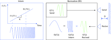
Figure 1: FMCW: Left increasing frequency chirp with slope K. Right: mixed frequencies

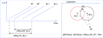
Figure 2: LPM Left: Offset difference between transponder MT, basis station BS and reference station RT. Right: LPM euclidian equation

The LPM was highly inspired by the FMCW frequency modulated continues wave radar (FMCW) and systems based on TOA, such as GPS. Figure 1 illustrates the functionality of a FMCW. The internal system is generating an increasing frequency chirp with a fixed slope K. This chirp is sent and reflected by an object. The received signal does not change its frequency, but during this time $(T2-T1)$ the internal frequency changed from $f1$ to $f2$. The radar can use an additive or multiplicative mixer to obtain the sum of the two frequencies and their differences. As only the frequency difference is required at this point, the frequency sum can be filtered by a low pass filter. The LPM is using this principle already, but in contrast to the FMCW radar, the send frequency chirp is getting compared with the frequency chirp of the other base station $KBS1=KBS2$ (figure 2). If the chirps are synchronized (started at the same time) there is no offset, but since the base stations and transponder are not synchronized, a reference station is required. Every frequency measurement the LPM provides is based on the difference between the transponder and one of the base stations with respect to the reference station at the same base station. Due to this fact, the time offset O is equal for every base station for the same measurement as demonstrated in fig. 2. This all leads to the LPM equation (1), with R: Pseudo Range, O: Offset, M: Transponder- and T: Reference station for different measurements i.

$$R_{i}=O+\left\|M-B_{i}\right\|-\left\|T-B_{i}\right\|$$ (1)

$$\left\|M-B_{i}\right\|=\sqrt{\left(x_{i}-x_{M}\right)^{2}+\left(y_{i}-y_{M}\right)^{2}}$$ (2)

$$\left\|T-B_{i}\right\|=\sqrt{\left(x_{i}-x_{T}\right)^{2}+\left(y_{i}-y_{T}\right)^{2}}$$ (3)

II Previous Work

The measurement principal of the Abatec LPM and its hardware implementation have been presented in [6] [9]. Previously published work about the LPM predominantly focused on the usage of Kalman filters to detect an outlier[3] or to track the position of the transponder [7]. An approach to outlier detection can be found in [3], were the linear Kalman filter in combination with the $\chi^{2}$ test was used to detect outliers within the offset corrupted data. Nonlinear equation solving with Bancroft is analyzed in [8][11] and compared with the least median of squares (LMS) in [2].

Abatec LPM (state-of-the-art):

• Solving of nonlinear TOA equation with a numerical solver.

• Unknown variables are coordinates of the transponder and the offset.

• Filtering after nonlinear multilateration.

New approach:

• TOA to TDOA transformation.

• The TDOA data is filtered before the multilateration.

• Both a linear TDOA solution and a nonlinear TDOA solution may be used to filter data before the lateration.

Advantages of new approach:

• Filtering before solving has the advantage that Gaussian noise inside of measurement data does not change due to numerical solver.

• The linear solution is faster than the nonlinear solution.

• The nonlinear solution does not have to fit the offset.

• Without the offset, outlier detection is enabled.

Disadvantage of new approach:

• The TDOA solution requires an additional base station

• The linear solution is more easily affected by unfavorable conditions .

III Methodology

The previous section introduced the LPM and the following focuses on its position estimation. In general, the exact positions of the reference station and base stations are known. In this way, four base stations are required to obtain the x, y, and z coordinates of the transponder. The euclidean form for this equation can be solved using either the Gauss-Newton method, or another non-linear solver. Alternatively, the equation may be linearized with a Taylor-series expansion [4] within a starting position. Unfortunately, in that case, the solution depends heavily on a good estimation of the starting condition. In order to detect the outlier and to obtain a strong starting conditions, one needs to analyze the data. The general approach for the LPM to detect an outlier was using Chi-test within a linear Kalman filter (LKF) [3] on raw data. Figure 3 shows that the offset ($O$) is $10^{6}$ times higher than the measurement itself. Furthermore, the offset is changing from one measurement to the next, due to the difference in oscillator clocks of reference station and transponder [3].The elimination of the offset allows us to see the relative range changing between the transponder and base station. This can be done by subtracting one base station from another at the same measurement. In figure 4 the result of this transformation on real measurements can be seen. The outliers are now visible with their typical characteristic of reflected data. At this point the TOA equation is changing to the TDOA. In [10] it was proven that the error propagation of the TDOA is equal to that of the TOA. This transformation can be done for two purposes: first, one may obtain the relative range between the base station and eliminate the offset; in this way we are able to filter data and outliers; second, one can rearrange the TOA equation to get the linear form of the transponder x, y, and z coordinates.

Figure 3: LPM real raw data with offset Z at different measurements

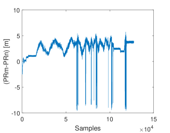
Figure 4: Pseudo range of the real data after the transformation

TOA to TDOA

III-A Linearization

Approaches such as the Taylor-series expansion [4] or other nonlinear solvers can be used to linearize the (1) equations. These methods require start information for the unknown variables. Alternatively one may use a reference station to obtain linear terms for the unknown position of the transponder. The offset will still be a part of the equation, but, just like the coordinates of the transponder, will be linear. This technique is also known as linear least squares multilateration. The main LPM equation (1) can be simplified by adding the known reference transponder range to the measurement term R (pseudo range).

$$L_{i}=R_{i}+\left\|T-B_{i}\right\|$$ (4)

$$\left\|M-B_{j}\right\|^{2}-\left\|M-B_{i}\right\|^{2}=\left(L_{j}-O\right)^{2}-\left(L_{i}-O\right)^{2}$$ (5)

The known quadratic terms of the transponder are eliminated, hence the linear solution for the transponder position at the known base station and reference station position is:

$$\left(\overrightarrow{B_{i}}-\overrightarrow{B_{j}}\right)\cdotp\overrightarrow{M}-\left(L_{i}-L_{j}\right)\cdotp O=$$

$$=\frac{1}{2}\left(\left(\left(\overrightarrow{B_{i}}\right)^{2}-\left(\overrightarrow{B_{j}}\right)^{2}\right)-\left(L_{i}^{2}-L_{j}^{2}\right)\right)$$ (6)

with

$$\begin{array}[]{cc}\overrightarrow{M}=\left(\begin{array}[]{c}x_{M}\\ y_{M}\end{array}\right)&\overrightarrow{B}=\left(\begin{array}[]{c}x_{B}\\ y_{B}\end{array}\right)\end{array}$$

The state-of-the-art Abatec LPM software uses a damped Newton iteration for nonlinear regression [11], requiring some start positions are required. The solution here presented, does not require any start position or nonlinear solvers. The method’s result, however, depends on the condition of the coefficient matrix (A). Should the pivots (diagonal elements of the coefficient matrix) be close to zero the condition is bad.

III-B Filtering

The transformation of the TOA to TDOA by subtracting one base station from a reference station can also be used to filter data. If equation 1 is not getting solved for T and squared before subtracted from a reference station, the term will still be nonlinear for the unknown position of the transponder, but the offset will be eliminated.
As mentioned above, every measurement has its offset, which is usually $10^{6}$ times higher than the location itself. If the numerical solver does not take this into account and the start conditions for the offset are unfavorable, then the changing in x, y, and z coordinates have almost no effect on the residuals. The higher the difference between $||M-B||$ and offset $O$ the higher the deviation between local optima and global optimum. Another problem could appear $R+||T\text{\textendash}B||>O$ in this case, the minimum of the numerical optimization becomes the maximum. The most suitable starting value for the offset would be the mean for every measurement, but we are still not able to set any start condition for the coordinates of the transponder or to interpret the measurements. In addition, the offset is changing from one measurement to the next, hence it promises suitable to use the difference between the base stations with respect to one reference station for the same measurement for further calculations. This method is known as the hyperbolic method [8] , due to the fact that the pseudorange is not maintained from the perspective of the transponder, if moving with a fixed radius on a circle around the basisstion, but in order to maintain the same pseudorange movement has to remain on a hyperbola. Changing the base station’s instead the of transponder’s position would provide a hyperbolic shape from the beginning. This shape is typical for TDOA, however, now the multidimensional damped Newton is utilized to solve the minimization of the equation [11]. Data may be filtered before position estimation, without the offset. The general approach for the LPM was to use the extended Kalman Filter, (EKF)[7] on the data provided by the numerical solver. But even if the data of the measurements has a gaussian noise, it does not necessarily mean that numerical output has a gaussian distribution as well. The least squares method to minimize the residuals $min\overset{n}{\underset{i=1}{\sum}}\frac{1}{2}(f(x,y,z)-y_{i})^{2}$is effected by outliers, but is able to deal with gaussian noise. A bad matrix condition or poorly chosen starting condition could lead to a result, which does not have a gaussian distribution anymore and therefore makes filtering the data before solving an advantage accompanied by a solver that does not have to estimate the offset. The solver converges faster and filtering can be one dimensional instead of three dimensional. The difference between the base stations to one reference station causes a dependency between the equations due to noise [1]. Based on empirical measurements, the variance of the noise (figure 5) for every base station differs from $0.003\,m{{}^{2}}$ to $0.0036\,m{{}^{2}}$ for an immobile transponder. Thus one can assume that the variance is equal for every base station. This is an important fact for iterative solving. There are several filters applicable to filtering the data in question. A very fast and simple filter is the moving average filter. This filter proves helpful when the focus lies on the time domain instead of the frequency domain. Its filter kernel (impulse response of the filter) does not require a convolution with a signal, instead, processing can be reduced to subtracting the oldest measurement and adding one of the latest measurements. Due to the central limit theorem, running the filter several times would lead to a similar result as using a convolution with a gaussian kernel. In this way the over and under oscillations of the frequency domain are reduced. The method is faster than the convolution with a Gaussian kernel. In figure 6 the result of the moving average filter, which is a Finite Impulse Response filter (FIR) illustrating the moving variance on real data after the transformation. All outliers have a high variance with respect to the other measurements. This information can be used not just to detect the transponder, but also the source of the reflection. The disadvantage of this method is a delay $(N-1)/2$ , which is increasing with the number of samples $N$. As an alternative, one could use the linear one dimensional Kalman filter instead. The difference between TOA and TDOA is visible (fig.7) Green circles represent the probability of the transponder location. Every circle represents one euclidean equation at a certain measurement. The correct location fits all the equations, therefore the residuals are the smallest. Smaller residuals are produced where just two equations fit, compared to other positions, hence the found coordinates are the local optimum (LO). The transformation results in simplified, hyperbola and triangles. The position of the transponder can be found by two hyperbola, but three hyperbola can be produced. The third can be represented by the other two, this hyperbola has no further information compared to the other two, but different local optima and another intersection angle. Due to this fact, numerical solving may influence, just by transforming, the probability to find a local optimum

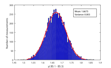
Figure 5: $BS_{1-3}$, Real data based gaussian distribution of the pseudo range difference for a not moving transponder

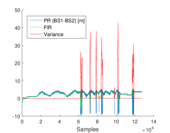
Figure 6: Example of reflection inside real data. Red curve represents variance, blue measurements and the green the filtered data

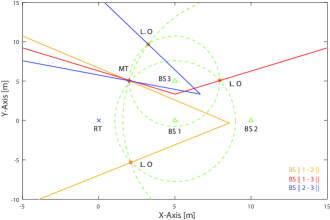
Figure 7: Difference between TOA and TDOA . The triangles are the simplified hyperboloids of TDOA and the green circles the euclidean form of TOA

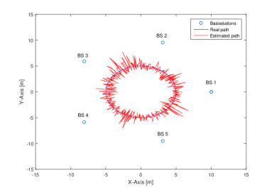
Figure 8: Synthetic data: Real path of transponder is located around the reference station with a radius of 5 m. The base stations have a distance of 10 m from the center and same distance to each other. Measurement data is corrputed by gaussian noise.

.

Combination of the linear equation with filtered data

The linear equation has some advantages over the nonlinear solution. This section presents a method of pre-filtering, which can be used to correct the linear solution. Tests showed that the noise is ten times higher than an immobile transponder, possibly due to the Doppler effect and the micro movements of the carrier. Therefore, we increased the random noise up to a maximum value of $0.1\,m$. The mean error of the estimated path with respect to the real path is $0.506\,m$ (fig. 8). The measurement L1 cannot be filtered as the time offset change with respect to time is $10^{6}$ times higher than the range change itself. Therefore, the offset is eliminated by subtracting one base station measurement from the other $(L_{i}-L_{j})$. In the next step this data is filtered over time. At this point it does not matter what kind of filter is used, it is only important that filtering takes place before position estimation and that the filter uses the measurement difference $(L_{i}-L_{j})$ as an input. For the following calculations we only assume that for every measurement we already have difference $(L_{i}-L_{j})$ the filtered values $F(L_{i}-L_{j})$ the main aim is to use the filtered values instead of the measurement differences between the base stations. The $(L_{i}^{2}-L_{j}^{2})$ term is nonlinear but the filtered values consist of the linear difference between the measurement ranges. One solution to using the filtered values would be to make every base station dependent on the same measurement error term $\alpha_{i}$. Every measurement is corrupted by the measurement error αi, hence the real measurement can be written as $L=\tilde{L}+\alpha$. The connection between the measurement errors αi and αj can be found if the unfiltered measurement difference $(L_{i}+\alpha_{i})-(L_{j}+\alpha_{j})$ is subtracted from the filtered values $F(L_{i}-L_{j})$.

$$F_{ij}=\left(\left(\tilde{L_{i}}+\alpha_{i}\right)-\left(\tilde{L_{j}}+\alpha_{j}\right)\right)-F\left(L_{i}-L_{j}\right)$$ (7)

$$\left(\tilde{L_{i}}-\tilde{L_{j}}\right)\thickapprox F\left(L_{i}-L_{j}\right)$$ (8)

The assumption that the noise can be neglected after the filtering, this leads to the term $F_{ij}$ being the difference between the noises of both signals.

$$F_{ij}=\alpha_{i}-\alpha_{j}$$ (9)

$$\alpha_{j}=-F_{ij}+\alpha_{i}$$ (10)

The measurement error is replaced by eq. 10.

$$\left(\overrightarrow{B_{i}}-\overrightarrow{B_{j}}\right)\cdotp\overrightarrow{M}-\left(\tilde{L_{i}}-\tilde{L_{j}}+F_{ij}\right)\cdotp O=$$

$$=\frac{1}{2}\left(\overrightarrow{B_{i}}^{2}-\overrightarrow{B_{j}}^{2}-\tilde{L_{i}}^{2}-\tilde{L_{j}}^{2}-F_{ij}^{2}\right.+$$

$$\left.+2\cdotp\alpha_{k}\left(\tilde{L_{i}}-\tilde{L_{j}}+F_{ij}\right)\right)$$

It can be observed that the time offset $O$, depends on the same parameters as the measurement error

$$\left(\overrightarrow{B_{i}}-\overrightarrow{B_{j}}\right)\cdotp\overrightarrow{M}-\left(\tilde{L_{i}}-\tilde{L_{j}}+F_{ij}\right)\cdotp\left(O+\alpha_{k}\right)=$$

$$=\frac{1}{2}\left(\overrightarrow{B_{i}}^{2}-\overrightarrow{B_{j}}^{2}-\tilde{L_{i}}^{2}-\tilde{L_{j}}^{2}-F_{ij}^{2}\right)$$

With at least four base stations, the unknown coordinates of the transponder can be estimated. With the filtered values the linear direct solution provides better results, than with the unfiltered equation $Ax=b$. This equation can be solved as:

$$\left(\begin{array}[]{c}x_{M}\\ y_{M}\\ O\end{array}\right)=\left(A^{T}A\right)^{-1}A^{T}b$$

Figure 9 presents the results of the new equation with noise. The mean error with a perfect filter is now below $10^{-11}\,m$. The experiment was repeated with synthetic data and a real moving average filter to investigate the behavior of outliers. Simulating a second base reflection the sample was set from 3500 to 3600 an outlier of 10 meters.

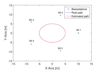
Figure 9: Noise correction

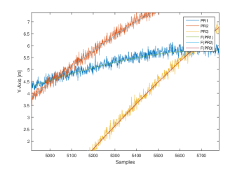
Figure 10: Synthetic data (PR) with gaussian noise and moving average filter F(PR)

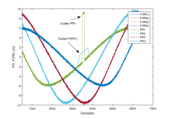
Figure 11: Filter error due to outlier: Such measurements are typical for signal reflections

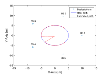
Figure 12: Outlier position estimation

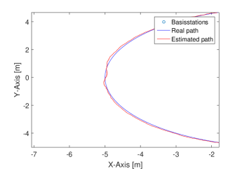
Figure 13: Result of the weighting on synthetic data with outlier

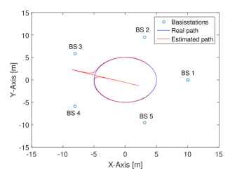
Figure 14: Result of weighting at unfavorable geometric condition

Figure 11 shows the results of the transformed signal and the filtered one (figure 10). The outlier causes some disturbance in the filtered output, which leads to an error in the position estimation (figure 12). This filter error can be minimized by taking variance into account. It is important to remember that the delay of the FIR filter to the signal is $(N-1)/2$ and of the moving variance $(N-1)/2$ plus the delay of the FIR, therefore we need some samples for the initialization and have no position estimation at the beginning (fig. 12). The provided variance is now used to obtain the weighting vector $w=1/var$.

$$\left(\begin{array}[]{c}w_{1}\\ \vdots\\ w_{n}\end{array}\right)Ax=\left(\begin{array}[]{c}w_{1}\\ \vdots\\ w_{n}\end{array}\right)b$$

The result of the weighting is visible in figure 13, the measurement with the highest error now has the smallest weight in the minimizing of the least squares problem. That being said, in applying a working filter eliminates the need for weights. Applying weighting at the position where the equation is sensitive to perturbations like $(PR_{m}-PR_{n}+RT_{m}-RT_{n})\approx 0$ or $B_{x},B_{y},B_{z}\approx 0$ the result of the position estimation will be highly inaccurate, due to corruption of the statistical meaning (fig. 14). In conclusion, we need to compare the nonlinear and the linear solution. Both methods have been transformed and filtered before the lateration. As a nonlinear solver we have used a Levenberg Marquardt method (LVM) [5]. The starting condition for the solver was the result of the previous fit beginning from the starting condition $x,y,z=0$ and fit parameter (table I). Due to the TOA to TDOA equation transformation, there is no need to fit the offset, for every step LVM x, y, and z coordinates of the transponder need to be estimated.

TABLE I: New linear parameter

Parameter	Value
Scaled gradient	0.000001
Relative function improvement	0.00001
Scaled step	0.001
Maximum iterations	20

Figure 15 presents the results of both methods. The linear solution has a slightly higher error rate compared to the nonlinear solution in some positions. The linear calculation, however, took $2596\,ms$ versus the nonlinear’s $4677\,ms$ on a i7-4600u CPU 2.10GHz and 16 GB Ram. It follows that if prefiltering would be a ‘perfect’ approach, both solutions would have the same result as the real path.

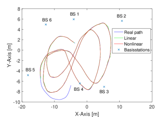
Figure 15: Linear and Nonlinear

IV Conclusions

The transformation from the TOA equation to the TDOA brings several advantages for the LPM. Section 3 demonstrated that the transformation leads to a linear equation, which can be solved without initialization and numerical iterations. Admittedly, the linear solution as compared to the nonlinear TDOA solution is more sensitive to perturbations given specific geometric settings. Obtaining the condition of the coefficient matrix, though, allows detection of these settings, and permitting use of the faster linear solution for every other position. The latter part of section 3 dealt with the TOA to TDOA transformation with the aim to eliminate the offset and to filter the data before the multilateration. Filtering the data before the position estimation, because non-linear function estimation leads to violation of normal distribution, made more sense, however. Furthermore, the transformation allowed the detection of outliers, reducing the number of local optima and decreasing the computational time due to the elimination of the offset. In the end, the linear solution was expanded with the possibility to use pre-filtered data and provide a solution at in half the time that a non-linear solution can.

References

- [1] Lukasz Zwirello et al. Uwb localization system for indoor applications: Concept, realization and analysis,. In Journal of Electrical and Computer Engineering, 2012.
- [2] Pfeil R et al. A robust position estimation algorithm for a local positioning measurement system. In Wireless Sensing, Local Positioning, and RFID, 2009. IMWS 2009. IEEE MTT-S International Microwave Workshop on, pages 1–4, Sept 2009.
- [3] R. Pfeil et al. Distributed fault detection for precise and robust local positioning. In In Proceedings of the 13th IAIN World Congress and Exhibition, 2009.
- [4] W. H. FOY. Position-location solutions by taylor-series estimation. IEEE Transactions on Aerospace and Electronic Systems, AES-12(2):187–194, March 1976.
- [5] Jorge J. Mor . The levenberg-marquardt algorithm: Implementation and theory. Numerical Analysis. Dundee, 1977.
- [6] K. Pourvoyeur, A. Stelzer, Alexander Fischer, and G. Gassenbauer. Adaptation of a 3-D local position measurement system for 1-D applications. In Radar Conference, 2005. EURAD 2005. European, pages 343–346, Oct 2005.
- [7] K. Pourvoyeur, A. Stelzer, T. Gahleitner, S. Schuster, and G. Gassenbauer. Effects of motion models and sensor data on the accuracy of the LPM positioning system. In Information Fusion, 2006 9th International Conference on, pages 1–7, July 2006.
- [8] K. Pourvoyeur, A. Stelzer, and G. Gassenbauer. Position estimation techniques for the local position measurement system LPM. In Microwave Conference, 2006. APMC 2006. Asia-Pacific, pages 1509–1514, Dec 2006.
- [9] A. Resch, R. Pfeil, M. Wegener, and A. Stelzer. Review of the LPM local positioning measurement system. In Localization and GNSS (ICL-GNSS), 2012 International Conference on, pages 1–5, June 2012.
- [10] Dong-Ho Shin and Tae-Kyung Sung. Comparisons of error characteristics between TOA and TDOA positioning. Aerospace and Electronic Systems, IEEE Transactions on, 38(1):307–311, Jan 2002.
- [11] A. Stelzer, K. Pourvoyeur, and A. Fischer. Concept and application of lpm - a novel 3-d local position measurement system. IEEE Transactions on Microwave Theory and Techniques, 52(12):2664–2669, Dec 2004.