Drag force in strongly coupled $\mathcal{N}=4$ SYM plasma in a magnetic field

Abstract

Applying AdS/CFT correspondence, we study the effect of a constant magnetic field $\mathcal{B}$ on the drag force associated with a heavy quark moving through a strongly-coupled $\mathcal{N}=4$ supersymmetric Yang-Mills (SYM) plasma. The quark is considered moving transverse and parallel to $\mathcal{B}$, respectively. It is shown that for transverse case, the drag force is linearly dependent on $\mathcal{B}$ in all regions. While for parallel case, the drag force increases monotonously with increasing $\mathcal{B}$ and also reveals a linear behavior in the regions of strong $\mathcal{B}$. In addition, we find that $\mathcal{B}$ has important effect for transverse case than parallel.

I Introduction

The experiments at Relativistic Heavy Ion Collider (RHIC) and Large Hadron Collider (LHC) have produced a new state of matter so-called quark gluon plasma (QGP) JA ; KA ; EV . One of the interesting properties of QGP is jet quenching: due to the interaction with the medium, high energy partons propagating through the QGP are strongly quenched. Usually, this phenomenon can be characterized by the jet quenching parameter which describes the average transverse momentum square transferred from the traversing parton, per unit mean free path. Alternately, the energy loss can also be analyzed from the drag force, which is related to the interaction between the moving quark and the medium. In the framework of weakly theories, the calculation of the jet quenching has been studied in many papers, see e.g. XN ; BG ; RB1 ; RB2 ; UA ; GLV ; SJ ; AMY . However, many experimental results indicate that QGP is strongly coupled EV . Thus, one would like to study the jet quenching in strongly coupled theory via the use of non-perturbative techniques, such as AdS/CFT Maldacena:1997re ; Gubser:1998bc ; MadalcenaReview .

AdS/CFT, the duality between the type IIB superstring theory formulated on AdS${}_{5}\times S^{5}$ and $\mathcal{N}=4$ SYM theory in four dimensions, has yielded many important insights for studying different aspects of QGP JCA . In this approach, the drag force for $\mathcal{N}=4$ SYM plasma was first investigated in CP ; GB . Therein, the energy loss of heavy quark is understood as the momentum flow along the string into the horizon. Later, this idea has been extended to various cases. For example, the effects of chemical potential on the drag force have been studied in ECA ; LC . The $R^{2}$ correction on the drag force have been discussed in KBF . The effects of constant B-field or non-commutativity on drag force have been investigated in TMA . Also, for the drag force in STU background, see JSA . For this quantity in some AdS/QCD models, see ENA ; PE ; UGU . Other important results can be found, for example, in DGI ; SCH ; MCH ; ANA ; KLP ; SRO ; SSG1 ; NA .

Now we would like to give such analysis under the influence of a magnetic field. The motivation comes from the experiment: the QGP produced in heavy-ion collisions may be subject to a strong electromagnetic field that created by many spectator nucleons DEK0 and the effect of a magnetic field on some topological DT ; KF ; DEK1 and the dynamical GSB ; KA1 ; DD ; RR properties of QGP have been investigated recently. On the other hand, one would like to be able to use holography to study the effect of the magnetic field on various quantities ED ; RCR ; KAMA ; RRO ; KIM ; SI ; SLI . Not long ago, the drag force in a strongly coupled $\mathcal{N}=4$ SYM plasma with a strong magnetic field has been discussed in KIM and the results show that this force is linearly dependent on $\mathcal{B}$, i.e., $f=-\frac{\sqrt{\lambda}\mathcal{B}}{6\pi}v$. However, the metric therein is valid only near the horizon, so the discussions are restricted to the infrared (IR) regime. In this paper, we would like to extend it to the case of all regimes by considering a general magnetic field. Specially, we want to know how an arbitrary magnetic field affects the drag force.

The paper is organized as follows. In the next section, we briefly review the asymptotic $AdS_{5}$ holographic Einstein-Maxwell model and introduce the background metric in the presence of a magnetic field. In section 3, we show numerical procedure and some numerical solutions. In section 4, we investigate the drag force for the quark moving transverse and parallel to the magnetic field, in turn. The last part is devoted to conclusion and discussion.

II Background geometry

The holographic model is Einstein gravity coupled with a Maxwell field, corresponding to strongly coupled $\mathcal{N}=4$ SYM subjected to a constant and homogenous magnetic field. The bulk action is ED

$$S=\frac{1}{16\pi G_{5}}\int d^{5}x\sqrt{-g}(R+\frac{12}{L^{2}}-F^{2})+S_{body},$$ (1)

where $G_{5}$ is the 5-dimensional gravitational constant, $L$ denotes the radius of the asymptotic $AdS_{5}$ spacetime. $F$ stands for the Maxwell field strength 2-form. Moreover, the term $S_{body}$ contains the Chern-Simons terms, Gibbons-Hawking terms and other contributions necessary for a well posed variational principle, but $S_{body}$ does not affect the solutions considered here.

The equations of motion for (1) are given by the Einstein equations

$$R_{\mu\nu}+\frac{4}{L^{2}}g_{\mu\nu}+\frac{1}{3}F_{\rho\sigma}F^{\rho\sigma}g_{\mu\nu}-2F_{\mu\rho}F_{\nu}^{\rho}=0,$$ (2)

and the Maxwell’s field equations

$$\nabla_{\mu}F^{\mu\nu}=0.$$ (3)

The ansatz for the magnetic brane geometry is ED

$$ds^{2}=-H(r)dt^{2}+e^{2P(r)}(dx^{2}+dy^{2})+e^{2V(r)}dz^{2}+\frac{dr^{2}}{H(r)},$$ (4)

with

$$F=Bdx\wedge dy,$$ (5)

where, for simplicity, we have set $L=1$. Note that in (4) the horizon is located at $r=r_{h}$ with $H(r_{h})=0$. The boundary is located at $r=\infty$. The constant $B$ refers to the bulk magnetic field, pointing in the $z$ direction. Also, the three coefficients $H(r)$, $P(r)$, and $V(r)$ can be obtained by solving the equations of motion.

In terms of (4), the Einstein equations reduce to

$$H(P^{\prime\prime}-V^{\prime\prime})+(H^{\prime}+H(2P^{\prime}+V^{\prime}))(P^{\prime}-V^{\prime})=-2B^{2}e^{-4P},$$ (6)

$$2P^{\prime\prime}+V^{\prime\prime}+2(P^{\prime})^{2}+(V^{\prime})^{2}=0,$$ (7)

$$\frac{1}{2}H^{\prime\prime}+\frac{1}{2}H^{\prime}(2P^{\prime}+V^{\prime})=4+\frac{2}{3}B^{2}e^{-4P},$$ (8)

$$2H^{\prime}P^{\prime}+H^{\prime}V^{\prime}+2H(P^{\prime})^{2}+4HP^{\prime}V^{\prime}=12-2B^{2}e^{-4P},$$ (9)

where the derivations are with respect to $r$. Unfortunately, for these coupled equations analytic solution can not be obtained easily. But an exact solution near the horizon ($r\sim r_{h}$), which denotes the product of a Banados, Teitelboim and Zanelli (BTZ) black hole times a two dimensional torus $T^{2}$, can be found as

$$ds^{2}=-\frac{r^{2}f(r)}{\mathcal{R}^{2}}dt^{2}+\mathcal{R}^{2}\mathcal{B}(dx^{2}+dy^{2})+\frac{r^{2}}{\mathcal{R}^{2}}dz^{2}+\frac{\mathcal{R}^{2}}{r^{2}f(r)}dr^{2},$$ (10)

with $f(r)=1-\frac{r_{h}^{2}}{r^{2}}$. Here $\mathcal{B}=\sqrt{3}B$ represents the physical magnetic field at the boundary and $\mathcal{R}=\frac{L}{\sqrt{3}}=\frac{1}{\sqrt{3}}$ denotes the radius of the BTZ black hole. It should be emphasized that the metric (10) is only valid near the horizon, i.e., in the regime $r<<\sqrt{\mathcal{B}}\mathcal{R}^{2}$ where the scale is much smaller than the magnetic field. Recently, several authors have used this metric to study the effect of strong magnetic field (IR regime) on the energy loss KIM and jet quenching parameter SLI .

In this article, rather than using (10), we apply a solution that interpolates between (10) in the IR and $AdS_{5}$ in the ultraviolet (UV). From the point of view of the boundary theory, this refers to an renormalization group (RG) flow between a $D=3+1$ CFT at small $r$ and a $D=1+1$ CFT at large $r$ ED . However, no analytic solution can be found in this case and one needs to resort to numerics. In the next section, we follow the numerical procedure mentioned in ED and present some numerical solutions.

III Numerical solutions

To begin with, we derive some useful equations. By eliminating the $B^{2}e^{-4P}$ terms in (6)$-$(9), we have

$$3H^{\prime\prime}+5(V^{\prime}+2P^{\prime})H^{\prime}+4({P^{\prime}}^{2}+2P^{\prime}V^{\prime})H-48=0,$$ (11)

$$3HP^{\prime\prime}+2H{P^{\prime}}^{2}-H^{\prime}P^{\prime}-5HP^{\prime}V^{\prime}+12-2H^{\prime}V^{\prime}=0,$$ (12)

$$3HV^{\prime\prime}+3H{V^{\prime}}^{2}+4H^{\prime}V^{\prime}+10HP^{\prime}V^{\prime}+2H{P^{\prime}}^{2}+2H^{\prime}P^{\prime}-24=0.$$ (13)

Following ED , it is convenient to use rescaled coordinates. First, we rescale $t\rightarrow\bar{t}$ , $r\rightarrow\bar{r}$ and fix the horizon at $\bar{r}_{h}=1$, so that

$$H(1)=0,\qquad H^{\prime}(1)=1.$$ (14)

In this case, the Hawking temperature is

$$T=\frac{\sqrt{-g^{\prime}_{\bar{t}\bar{t}}g^{\bar{r}\bar{r}\prime}}}{4\pi}\big{|}_{\bar{r}=1}=\frac{1}{4\pi}.$$ (15)

Next we rescale $x$, $y$, $z$ coordinates to have

$$P(1)=V(1)=0,\qquad P^{\prime}(1)=4-\frac{b^{2}}{3},\qquad V^{\prime}(1)=4+\frac{b^{2}}{6},$$ (16)

where $b$ stands for the value of the magnetic field in the rescaled coordinates. Notice that if $P^{\prime}<0$, the geometry will not be asymptotically $AdS_{5}$, thus, the second equation in (16) gives us $0\leq b<2\sqrt{3}$.

Moreover, the geometry will have the asymptotic behavior as $\bar{r}\rightarrow\infty$,

$$H(\bar{r})\rightarrow\bar{r}^{2},\qquad e^{2P(\bar{r})}\rightarrow m(b)\bar{r}^{2},\qquad e^{2V(\bar{r})}\rightarrow n(b)\bar{r}^{2},$$ (17)

where $m(b)$ and $n(b)$ are rescaling parameters which can be determined numerically. Also, the physical magnetic field $B_{0}$ is given by

$$B_{0}=\sqrt{3}\frac{b}{m(b)}.$$ (18)

Actually, the interval of $b$ can be obtained from (18) as well. One can numerically check that $m(b)$ is a decreasing function of $b$ and $m(b\rightarrow 2\sqrt{3})\rightarrow 0$, for this behavior, see in the left panel of fig.1. On the other hand, it implies that one covers in practice all values of $B_{0}$ for $0\leq b<2\sqrt{3}$.

Finally, to have an asymptotic $AdS_{5}$ in the UV, one needs to rescale back to the original coordinate system by setting $(\bar{x},\bar{y},\bar{z})\rightarrow(x/\sqrt{m(b)},y/\sqrt{m(b)},z/\sqrt{n(b)}$, then metric (4) becomes

$$ds^{2}=-H(\bar{r})dt^{2}+\frac{e^{2P(\bar{r})}}{m(b)}(dx^{2}+dy^{2})+\frac{e^{2V(\bar{r})}}{n(b)}dz^{2}+\frac{dr^{2}}{H(\bar{r})}.$$ (19)

When this is done, one can solve the coupled equations (11)$-$(13) with the boundary conditions (14) and (16). As a matter of convenience, we drop from now on the bars in the rescaled coordinates. The numerical procedure can be summarized as follows: First, choosing a value of $b$ for $0\leq b<2\sqrt{3}$, one solves the equations (11)$-$(13) and obtains the numerical solutions of $H(r),P(r)$ and $V(r)$. Then, fitting the asymptotic data for $e^{2P(r)}\rightarrow m(b)r^{2}$ and $e^{2V(r)}\rightarrow n(b)r^{2}$, one gets the values of $m(b)$ and $n(b)$. Then the value of $B_{0}$ can be obtained from (18). Finally, setting $(e^{2P(r)},e^{2V(r)})\rightarrow(e^{2P(r)}/m(b),e^{2V(r)}/n(b))$, one obtains the numerical solutions. Likewise, one can study other cases by varying the value of $b$ . In the right panel of fig.1, we plot $\ln H(r),P(r)$, $V(r)$ versus $r$ for $b=2.7$, we have checked that it matches the fig.3 in RRO .

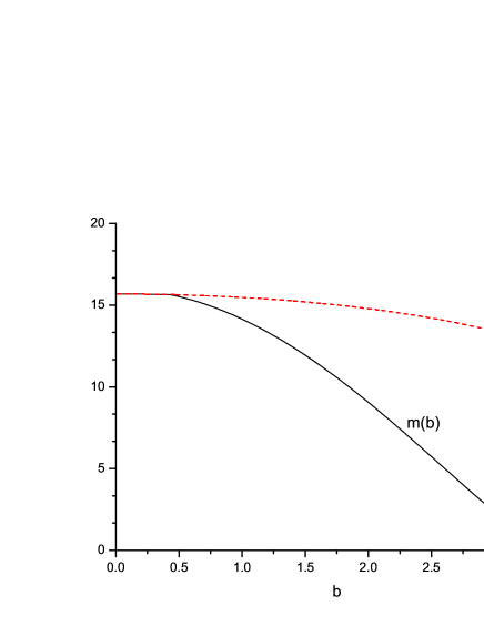
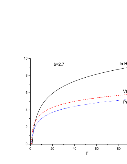
Figure 1: Left: $n(b)$ (dash curve) and $m(b)$ (solid curve) against $b$. Right: $\ln H(r)$ (solid curve), $V(r)$ (dash curve) and $P(r)$ (dot curve) against $r$ for $b=2.7$.

IV drag force

It is known that when a heavy quark moves in a hot medium, its interaction with the medium leads to a drag force thus making it losing energy. On the other hand, the energy loss can be depicted in a dual trailing string picture CP ; GB , that is, a heavy quark moving on the boundary, but with a string tail into the AdS bulk. Under this scenario, the dissipation of the heavy quark could be described by the drag force, which is conjectured to be associated with a string tail in the fifth dimension.

In the proposal of CP ; GB , the drag force is related to the damping rate $\mu$ (or friction coefficient), defined by Langevin equation,

$$\frac{dp}{dt}=-\mu p+f_{1},$$ (20)

subject to a driving force $f_{1}$. And, for constant speed trajectory (or $dp/dt=0$), the driving force is equivalent to a drag force $f$.

Generally, to discuss the magnetic effect, one needs to consider different alignments for the velocity with respect to the direction of the magnetic field, i.e., transverse ($\theta=\pi/2$), parallel ($\theta=0$), or arbitrary direction ($\theta$). Here we consider two cases: transverse and parallel.

IV.1 Transverse case ($\theta=\pi/2$)

First we study the quark moving perpendicularly to the magnetic field in the $x$ direction. The coordinates are parameterized by

$$t=\tau,\qquad x=vt+\xi(r),\qquad y=0,\qquad z=0,\qquad r=\sigma,$$ (21)

where one end point of the trailing string moves with the velocity $v$ on the boundary while the other parts move in the bulk.

The string dynamic is governed by the Nambu-Goto action

$$S=-\frac{1}{2\pi\alpha^{\prime}}\int d\tau d\sigma\sqrt{-g},$$ (22)

where $g$ is the determinant of the induced metric with

$$g_{\alpha\beta}=g_{\mu\nu}\frac{\partial X^{\mu}}{\partial\sigma^{\alpha}}\frac{\partial X^{\nu}}{\partial\sigma^{\beta}},$$ (23)

where $g_{\mu\nu}$ and $X^{\mu}$ represent the brane metric and target space coordinates, respectively. Moreover, $\alpha^{\prime}$ is related to the ’t Hooft coupling by $1/\alpha^{\prime}=\sqrt{\lambda}$.

Plugging (21) into (4), the induced metric reads

$$g_{tt}=-H(r),\qquad g_{xx}=e^{2P(r)},\qquad g_{rr}=\frac{1}{H(r)},$$ (24)

given this, one can identify the lagrangian density as

$$\mathcal{L}=\sqrt{-g_{rr}g_{tt}-g_{rr}g_{xx}v^{2}-g_{xx}g_{tt}{\xi^{\prime}}^{2}}=\sqrt{1-\frac{e^{2P(r)}}{H(r)}v^{2}+e^{2P(r)}H(r){\xi^{\prime}}^{2}},$$ (25)

with $\xi^{\prime}=d\xi/d\sigma$.

The equation of motion implies that $\frac{\partial L}{\partial\xi^{\prime}}$ is a constant. If one calls it $\Pi_{\xi}$, then

$$\Pi_{\xi}=\frac{\partial L}{\partial\xi^{\prime}}=-\xi^{\prime}\frac{g_{tt}g_{xx}}{\sqrt{-g}}=\xi^{\prime}\frac{H(r)e^{2P(r)}}{\sqrt{1-\frac{e^{2P(r)}}{H(r)}v^{2}+e^{2P(r)}H(r){\xi^{\prime}}^{2}}},$$ (26)

results in

$${\xi^{\prime}}^{2}=\frac{{\Pi_{\xi}}^{2}[1-\frac{v^{2}e^{2P(r)}}{H(r)}]}{H(r)e^{2P(r)}[H(r)e^{2P(r)}-{\Pi_{\xi}}^{2}]},$$ (27)

note that in the right hand of (27), near the horizon the denominator and numerator are both positive for large $r$ and negative for small $r$. In addition, it is required that ${\xi^{\prime}}^{2}$ must be everywhere positive. Thus, the denominator and numerator should change sigh at the same point, which leads to

$$H(r_{c})=e^{2P(r_{c})}v^{2},$$ (28)

and

$${\Pi_{\xi}}^{2}=H(r_{c})e^{2P(r_{c})},$$ (29)

where $r=r_{c}$ is the critical point.

On the other hand, the current density for momentum $p_{1}$ along the $x$ direction can be written as

$$\pi_{x}^{r}=-\frac{1}{2\pi\alpha^{\prime}}\xi^{\prime}\frac{g_{tt}g_{xx}}{-g}.$$ (30)

As a result, the drag force is obtained as

$$f_{b}=\frac{dp_{1}}{dt}=\sqrt{-g}\pi_{x}^{r}=-\frac{1}{2\pi\alpha^{\prime}}{\Pi_{\xi}}=-\frac{1}{2\pi\alpha^{\prime}}ve^{2P(r_{c})},$$ (31)

where the minus sign means that the direction of the drag force is against the movement.

To compare with the strong magnetic field case in KIM , we set $e^{2P(r_{c})}=\mathcal{R}^{2}\mathcal{B}=\frac{1}{3}\mathcal{B}$ in (31). After using the relation $1/\alpha^{\prime}=\sqrt{\lambda}$, one gets

$$\frac{dp_{1}}{dt}=-\frac{\sqrt{\lambda}\mathcal{B}}{6\pi}v,$$ (32)

which is exactly Eq.(32) in KIM .

Also, if one sets $H(r)=\frac{r^{2}}{L^{2}}(1-\frac{r_{h}^{4}}{r^{4}})$, $e^{2P(r)}=e^{2V(r)}=\frac{r^{2}}{L^{2}}$ in (4), the drag force for $\mathcal{N}=4$ case CP ; GB can be obtained from (31), that is

$$f_{\mathcal{N}=4}=-\frac{\pi T^{2}\sqrt{\lambda}}{2}\frac{v}{\sqrt{1-v^{2}}},$$ (33)

where we have used the relations

$$L^{4}=\lambda{\alpha^{\prime}}^{2},\qquad r_{h}=\pi L^{2}T.$$ (34)

To proceed, we study the effect of magnetic field on the drag force for the transverse case. Numerically, we plot the absolute value of the drag force versus $B_{0}/T^{2}$ in the left panel of fig.2. (Since our main interest is to consider the magnetic field effect, the coefficient $\frac{1}{2\pi\alpha^{\prime}}$ does not play any role, here we set it as unity). From the figures, one can see that at fixed velocity the drag force is almost linearly dependent on $B_{0}/T^{2}$. Especially, the linear behavior is quite well for the regions of strong magnetic field, in accordance with KIM . Moreover, by comparing the two figures, one finds that at fixed magnetic field, the drag force increases as the velocity increases.

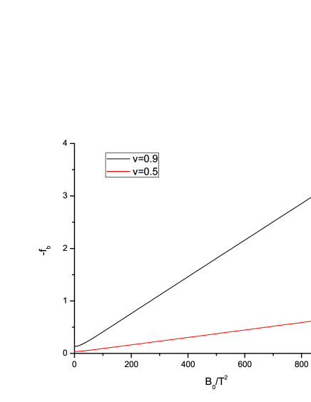
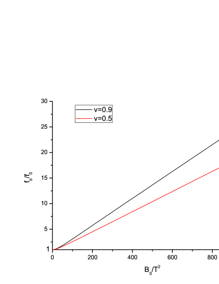
Figure 2: Left: ${-f_{b}}$ against $B_{0}/T^{2}$ for $\theta=\pi/2$. Right: ${f_{b}}/{f_{0}}$ against $B_{0}/T^{2}$ for $\theta=\pi/2$. In all of the plots from top to bottom, $v=0.9,0.5$, respectively. Here the velocity of light is taken as $c=1$.

On the other hand, one can compare the drag force between the cases of $b\neq 0$ and $b=0$ as following,

$$\frac{f_{b}}{f_{0}}=\frac{(\frac{dp_{1}}{dt})_{b}}{(\frac{dp_{1}}{dt})_{b=0}}=\frac{\frac{e^{2P(r_{c})}}{m(b)}|_{b}}{\frac{e^{2P(r_{c})}}{m(b)}|_{b=0}},$$ (35)

the plots of ${f_{b}}/{f_{0}}$ versus $B_{0}/T^{2}$ for two different velocities are presented in the right panel of fig.2. One can see that it also reveals a linear behavior. Therefore, one concludes that for the transverse case, the drag force increases linearly with the increase of the magnetic field.

IV.2 Parallel case ($\theta=0$)

In this subsection we discuss the heavy quark moving parallel to the magnetic field in the $z$ direction. The coordinates are parameterized by

$$t=\tau,\qquad x=0,\qquad y=0,\qquad z=vt+\xi(r).\qquad r=\sigma.$$ (36)

The next analysis is very similar to the transverse case, so we present the final results. The drag force for the parallel case is

$$f_{b}^{\prime}=\frac{dp_{2}}{dt}=\sqrt{-g^{\prime}}\pi_{z}^{r}=-\frac{1}{2\pi\alpha^{\prime}}ve^{2V(r_{c})},$$ (37)

where $r_{c}$ satisfies

$$H(r_{c})=e^{2V(r_{c})}v^{2}.$$ (38)

Likewise, we plot ${-f_{b}^{\prime}}$ versus $B_{0}/T^{2}$ and ${f_{b}^{\prime}}/{f_{0}}$ versus $B_{0}/T^{2}$ in fig.3. From the figures, one finds that the drag force monotonously increases as the magnetic field increases. Also, it reveals a linear behavior for the regime of strong magnetic field. In addition, by comparing fig.2 and fig.3, one can see that the slope of the plot in the parallel case is much less than its counterpart in the transverse case, which means that the magnetic field has important effect for the transverse case. Interestingly, a similar observation has been found in RRO which indicates that the magnetic field has stronger effect on the heavy quark potential for the perpendicular configuration.

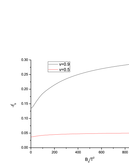
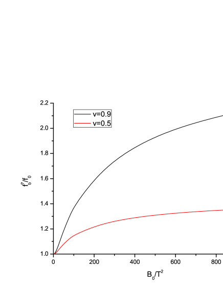
Figure 3: Left: ${-f_{b}^{\prime}}$ against $B_{0}/T^{2}$ for $\theta=0$. Right: ${f_{b}^{\prime}}/{f_{0}}$ against $B_{0}/T^{2}$ for $\theta=0$. In all of the plots from top to bottom, $v=0.9,0.5$, respectively. Here the velocity of light is taken as $c=1$.

Several comments are in order: First, the rate of energy loss $\frac{dE}{dt}=\bar{{f}}\cdot\bar{v}$ is dependent on the magnetic field, and a strong magnetic field also yields a linear behavior, in agreement with KIM . On the other hand, it is known that the drag force is a kind of viscous force, since the magnetic field has the effect of increasing the drag force, one can say that the magnetic field makes the medium more viscous. One step further, the magnetic field increases the effective viscosity of QGP to a heavy quark.

V conclusion and discussion

Motivated by the recent studies which regarding the influence of a strong magnetic field on QGP, in this paper, we analyzed the effect of a constant magnetic field on the drag force with respect to a heavy quark moving in a strongly-coupled $\mathcal{N}=4$ SYM plasma. We considered the quark moving transverse and parallel to the magnetic field, respectively. It is shown that for transverse case, the drag force is linearly dependent on the magnetic field. While for parallel case, the drag force monotonously increases as the magnetic field increases, and in the regions of strong magnetic field it also reveals a linearly behavior, which supports the findings of KIM . In addition, we find that the magnetic field has a stronger effect for transverse case rather than parallel.

On the other hand, the results indicate that the magnetic field increases the effective viscosity of QGP. Interestingly, this finding is contrast to that in TMA . But one should keep in mind that the two results come from two different holographic models. In TMA , the authors consider a non-magnetized plasma (ignoring the effect of the magnetic field on the plasma) and discuss the effect of constant B-field or non-commutativity. In this article, we consider a strongly coupled $\mathcal{N}=4$ SYM plasma in the presence of a constant magnetic field. In short, the later is closer to practical KIM .

Certainly, one should bear in mind that $\mathcal{N}=4$ SYM and QCD are different theories, in particular, in the vacuum. But at finite temperature the two theories appear less different. So the results obtained from $\mathcal{N}=4$ SYM plasma may shed some light to QGP.

Finally, it should be noticed that the plasma considered here is with zero chemical potential and finite magnetic field. So one can take account into finite density in this model as well. It is relevant to mention that the charged magnetic brane solutions has been discussed in ED1 . Using that metric, one can study the effects of both chemical potential and finite magnetic field on the drag force. We leave this for further study.

VI Acknowledgments

The authors would like to thank the anonymous referee for his/her valuable comments and helpful advice. This work is partly supported by the Ministry of Science and Technology of China (MSTC) under the 973 Project No. 2015CB856904(4). Z-q Zhang is supported by NSFC under Grant No. 11705166. D-f. Hou is supported by the NSFC under Grants Nos. 11735007, 11521064.

References

- (1) J. Adams et al. [STAR Collaboration], Nucl. Phys. A 757, 102 (2005).
- (2) K. Adcox et al. [PHENIX Collaboration], Nucl. Phys. A 757, 184 (2005).
- (3) E. V. Shuryak, Nucl. Phys. A 750, 64 (2005).
- (4) X. N. Wang and M. Gyulassy, Phys. Rev. Lett. 68, 1480 (1992).
- (5) B. G. Zakharov, JETP Lett. 63, 952 (1996).
- (6) R. Baier, Y. L. Dokshitzer, A. H. Mueller, S. Peigne and D. Schiff, Nucl. Phys. B 484, 265 (1997).
- (7) R. Baier, Y.L. Dokshitzer, A.H. Mueller and D. Schiff, JHEP 09 (2001) 033.
- (8) U. A. Wiedemann, Nucl. Phys. B 588, 303 (2000).
- (9) M. Gyulassy, P. Levai and I. Vitev, Phys. Rev. Lett. 85, 5535 (2000).
- (10) S. Jeon and G.D. Moore, Phys. Rev. D 71 (2005) 034901.
- (11) P. Arnold, G. D. Moore and L. G. Yaffe, JHEP 0111, 057 (2001).
- (12) J. M. Maldacena, Adv. Theor. Math. Phys. 2, 231 (1998).
- (13) S. S. Gubser, I. R. Klebanov and A. M. Polyakov, Phys. Lett. B 428, 105 (1998).
- (14) O. Aharony, S. S. Gubser, J. Maldacena, H. Ooguri and Y. Oz, Phys. Rept. 323, 183 (2000).
- (15) J. Casalderrey-Solana, H. Liu, D. Mateos, K. Rajagopal and U. A. Wiedemann, arXiv:1101.0618
- (16) C. P. Herzog, A. Karch, P. Kovtun, C. Kozcaz and L. G. Yafe, JHEP 07 (2006) 013.
- (17) S. S. Gubser, Phys.Rev.D 74 126005 (2006).
- (18) E. Caceres and A. Guijosa, JHEP 11 (2006) 077.
- (19) L. Cheng, X.-H. Ge and S.-Y. Wu, Eur.Phys.J. C 76 256 (2016).
- (20) K. B. Fadafan, JHEP 12 (2008) 051.
- (21) T. Matsuo, D. Tomino and W.-Y. Wen, JHEP 10 (2006) 055.
- (22) J. Sadeghi, M. R. Setare, B. Pourhassan and S. Hashmatian, Eur.Phys.J.C 61 527 (2009).
- (23) E. Nakano, S. Teraguchi and W.-Y. Wen, Phys. Rev. D 75 (2007) 085016.
- (24) P. Talavera, JHEP 0701 (2007) 086.
- (25) U. Gursoy, E. Kiritsis, G. Michalogiorgakis and F. Nitti, JHEP 0912 (2009) 056.
- (26) D. Giataganas, JHEP 1207 (2012) 031.
- (27) S. Chakraborty, N. Haque, JHEP 1412 (2014) 175.
- (28) M. Chernicoff, D. Fernandez, D. Mateos and D. Trancanelli, JHEP 1208 (2012) 100.
- (29) A. N. Atmaja and K. Schalm, JHEP 1104 (2011) 070.
- (30) K. L. Panigrahi and S. Roy, JHEP 1004 (2010) 003.
- (31) S. Roy, Phys. Lett. B 682 93 (2009).
- (32) S. S. Gubser, Phys. Rev. D 76 (2007) 126003.
- (33) N. Abbasi, A. Davody JHEP 1206 (2012) 065.
- (34) D. E. Kharzeev, L. D. McLerran, and H. J. Warringa, Nucl. Phys. A 803, 227 (2008).
- (35) D. T. Son and A. R. Zhitnitsky, Phys. Rev. D 70, 074018 (2004).
- (36) K. Fukushima, D. E. Kharzeev, and H. J. Warringa, Phys. Rev. D 78, 074033 (2008).
- (37) D. E. Kharzeev and H. U. Yee, Phys. Rev. D 83, 085007 (2011).
- (38) G. S. Bali, F. Bruckmann, G. Endrodi, Z. Fodor, S. D. Katz, S. Krieg, A. Schaer, and K. K. Szabo, JHEP 02 (2012) 044.
- (39) K. A. Mamo, JHEP 05 (2015) 121.
- (40) D. Dudal, D. R. Granado, and T. G. Mertens, Phys. Rev. D 93, 125004 (2016).
- (41) R. Rougemont, R. Critelli, and J. Noronha, Phys. Rev. D 93, 045013 (2016).
- (42) E. D. Hoker and P. Kraus, JHEP 10 (2009) 088.
- (43) R. Critelli, S. I. Finazzo, M. Zaniboni, and J. Noronha, Phys. Rev. D 90, 066006 (2014).
- (44) K. A. Mamo, JHEP 08 (2013) 083.
- (45) R. Rougemont, R. Critelli and J. Noronha, Phys. Rev. D 91, 066001 (2015).
- (46) K. A. Mamo, Phys. Rev. D 94, 041901(R) (2016).
- (47) S. I. Finazzo, R. Critelli, R. Rougemont and J. Noronha, Phys. Rev. D 94, 054020 (2016).
- (48) S. Li, K. A. Mamo and H.U.Yee, Phys. Rev. D 94, 085016 (2016).
- (49) E. D. Hoker and P. Kraus, JHEP 03 (2010) 095.