Programming infinite machines

Abstract

For infinite machines which are free from the classical Thompson’s lamp paradox we show that they are not free from its inverted version. We provide a program for infinite machines and an infinite mechanism which simulate this paradox. While their finite analogs work predictably, the program and the infinite mechanism demonstrate an undefined behavior. As in the case of infinite Davies’s machines, our examples are free from infinite masses, infinite velocities, infinite forces, etc. Only infinite divisibility of space and timeis assumed. Thus, the considered infinite devices are possible in a continuous Newtonian Universe and they do not conflict with continuous Newtonian mechanics. Some possible applications to the analysis of the Navier-Stokes equations are discussed.

I Introduction

The classical Thompson’s lamp paradox appears in T1 . Let us provide its computer interpretation. Suppose that we have one byte $a$ of memory and some CPU which can carry out an infinite number of operations within a finite length of time. Consider the following set of instructions (so-called Zeno process)

$t=0:$    $a:=0;$

$t=1/2:$   $a:=1;$

$t=3/4:$   $a:=0;$

$t=7/8:$    $a:=1;$

….,

where $t$ is time. Assuming that CPU time of each next operation is twice faster than the CPU time of a previous operation, we can write a pascal code for the Thompson’s program

$a:=0;$

$\rm REPEAT$

$a:={\rm not}\ a;$

$\rm UNTIL\ FALSE;$

The paradox is that, we can not predict or determine the value of $a$ after the time $t$ when all operations are completed. For the first example, this time is $t=1$.

The theoretical description of infinite machines appears in BBJ1 ; H1 . The possibility of producing of such machines in certain exotic relativistic spacetimes (sometimes called Hogarth-Malament spacetimes) is demonstrated in EN1 . The construction of infinite machines in a continuous Newtonian Universe is discussed in D1 . In D1 , it is mentioned that the proposed infinite machine is free from the Thomson paradox. In this paper we show that such infinite machine is not free from the inverted Thompson’s paradox. The rough idea of this paradox consists of changing the order of operations in the classical Thompson’s paradox.

This topic is also closely related to the physical Church-Turing thesis which is the conjecture that no computing device that is physically realizable can exceed the computational barriers of a Turing machine, see, e.g., W ; ND ; S . The result of the paper confirms this thesis since the infinite Davies’s machine, which allows a hypercomputation, demonstrates also an unpredictable behaviour. This raises doubts about the fundamental possibility of constructing this machine and other hypercomputers (even without taking into account the quantum nature of the real world). Moreover, it indicates some fundamental difficulties in a continuous Newtonian Universe itself. In particular, this observation may be helpful in analysis of Newtonian fluid dynamics, e.g. in analysis of the Navier-Stokes equations. For example, if a fluid analog of the mechanism considered in Section IV exists in a continuous Newtonian Universe then the Navier-Stokes equations do not have a unique solution since the mechanism demonstrates an undefined behavior. It is known that fluid motions can be very complex, see, e.g. FS . They can create arbitrary small eddies and turbulent vortices with bizarre shapes. All this allows us to hope for the possibility of constructing the fluid analogs that will be close in some properties to the mechanism depicted on Fig. 4. Then, it can be perspective for presenting a negative answer to the ”millenium problem”.

Another useful information about the physical Church-Turing thesis along with hypercomputation and supertask can be found in CR ; C1 ; HK ; C2 ; N1 . It is also useful to note the paradox called ”paradox of predictability” or ”second oracle paradox”, see, e.g. RC . The infinite analog of the paradox of predictability has some similar features with the inverted Thompson paradox. The corresponding analysis will be presented elsewhere.

The paper is organized as follows. Sections II,III contain the description of the infinite machine and the program ”puzzle” which demonstrates unpredictable behavior. Section IV contains the description of a pure mechanical device which demonstrates the same undefined behavior as the program ”puzzle”. We conclude in Section V.

II The construction

We consider a simplified version of infinite machine from D1 . The machine ${\mathscr{M}}=\cup_{n=1}^{\infty}{\mathcal{M}}_{n}$ consists of infinite number of finite machines ${\mathcal{M}}_{n}$, $n\in{\mathbb{N}}$, see Fig. 1. The machine ${\mathcal{M}}_{n+1}$ is a small copy of the machine ${\mathcal{M}}_{n}$ for all $n$. The machine ${\mathcal{M}}_{n+1}$ is also twice faster than the machine ${\mathcal{M}}_{n}$ for all $n$. For instance, we assume that CPU time $\tau_{n}$ of ${\mathcal{M}}_{n}$ is equal to $1/2^{n}$ for all $n$. We do not assume that the memory of ${\mathcal{M}}_{n+1}$ is large than the memory of ${\mathcal{M}}_{n}$. All machines have the same memory size, say $1$ byte for data and $1$ Kbyte for a program code and for built-in variables. Single-threaded CPU (interpreter) of each ${\mathcal{M}}_{n}$ can perform integer and logic operations and simple data manipulations. Each ${\mathcal{M}}_{n}$ can interact directly with adjacent ${\mathcal{M}}_{n+1}$ only.

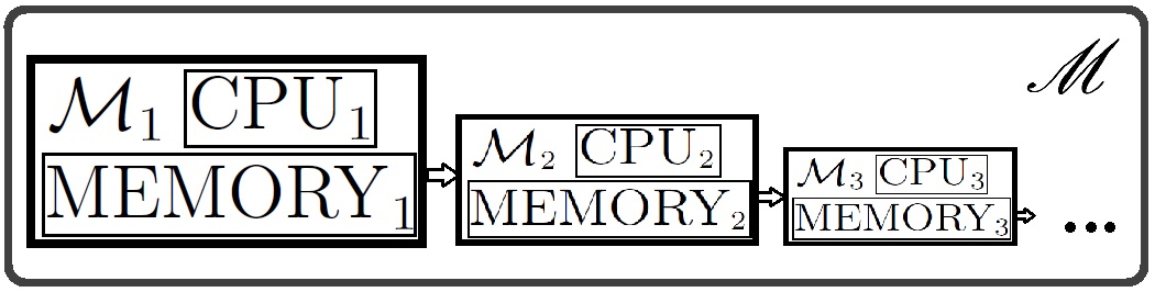
Figure 1: The structure of the infinite machine ${\mathscr{M}}$.

Let us describe some commands of the machine ${\mathscr{M}}$. If CPU of the machine ${\mathcal{M}}_{n}$ gets the instruction

$${\rm COPY\_PROGRAM\_NEXT}\ something;$$

then it copies the code placed between ”${\rm PROGRAM}\ something:$” and ”${\rm END}\ something;$” to the program memory of ${\mathcal{M}}_{n+1}$ and runs the copy there. The instruction

$${\rm IDLE}\ m;$$

says that CPU should skip $m$ CPU time’s $\tau_{n}$ before executing next instructions. CPU time $\tau_{n}(=1/2^{n})$ depends on the machine ${\mathcal{M}}_{n}$, where the instruction ${\rm IDLE}$ is performed. Any ${\mathcal{M}}_{n}$ has built-in variables:

$${\rm VALUE}$$

which refers to the byte data memory of ${\mathcal{M}}_{n}$, and

$${\rm VALUE\_NEXT}$$

which refers to the byte data memory of ${\mathcal{M}}_{n+1}$. At the beginning of a program, all values are initialized to $0$. This remark is very important in the program ”puzzle” considered below. The instructions

$${\rm NOT},\ \ \ :=$$

mean the bitwise ”not” and the assignment operation respectively. In particular, $({\rm NOT}\ 1)=0$ and $({\rm NOT}\ 0)=1$. We assume that all instructions described above (except ${\rm IDLE}$) take one CPU time $\tau_{n}$ for performing. The CPU time $\tau_{n}(=1/2^{n})$ depends on the machine ${\mathcal{M}}_{n}$, where the instruction is performed.

The machine ${\mathscr{M}}$ is free from the classical Thompson’s paradox because the CPU-s can not manipulate with the fixed memory cell an infinite number of times. Nevertheless, ${\mathscr{M}}$ is not free from the inverted Thompson’s paradox.

III The puzzle

The following program emulates the inverted Thompson’s paradox. The code is written in a pascal-based programming language. The comments are placed in parentheses $\{...\}$.

$$\begin{array}[]{ll}{\rm PROGRAM}\ puzzle:&\{entry\ point\}\\ {\rm COPY\_PROGRAM\_NEXT}\ puzzle;&\{instruction\ 1\}\\ {\rm IDLE}\ 2;&\{instruction\ 2\}\\ {\rm VALUE}:={\rm NOT}\ {\rm VALUE\_NEXT};&\{instruction\ 3\ (two\ instructions)\}\\ {\rm END}\ puzzle;&\{exit\}\end{array}$$

The program starts on ${\mathcal{M}}_{1}$, copies to ${\mathcal{M}}_{2}$ and starts there, waits for some time, takes the ”inverted” value from ${\mathcal{M}}_{2}$ and stops. The same happens in ${\mathcal{M}}_{2}$, ${\mathcal{M}}_{3}$, and so on. In fact, the program works like a shader for a multiprocessor system. The corresponding time diagram is plotted in Fig. 2. Let us denote the time when $i$-th instruction ($i=1,2,3$) starts on ${\mathcal{M}}_{n}$ ($n\in{\mathbb{N}}$) by $t_{ni}$. Let us denote the exit time on ${\mathcal{M}}_{n}$ by $t_{n4}$, $n\in{\mathbb{N}}$. Then

$$t_{n1}=\sum_{m=1}^{n-1}\tau_{m}=1-2^{1-n},\ \ \ t_{n2}=t_{n1}+\tau_{n}=1-2^{-n},\\ t_{n3}=t_{n2}+2\tau_{n}=1+2^{-n},\ \ \ t_{n4}=t_{n3}+2\tau_{n}=1+2^{-n}+2^{1-n}.$$ (1)

Due to (1), all values will be initialized and there are no conflicts between parallel programs working on different ${\mathcal{M}}_{n}$, since only adjacent machines can interact. Nevertheless, we can not determine the value on ${\mathcal{M}}_{1}$ at the end of the program ”puzzle”. The reason is similar as in the inverted Thomson paradox. Both values ${\rm VALUE}_{1}=0$ and ${\rm VALUE}_{1}=1$ are possible (and impossible) at the end of the program. More precisely, if we execute ”puzzle” on the finite machine ${\mathscr{M}}_{N}=\cup_{n=1}^{N}{\mathcal{M}}_{n}$ (the cascade stops in ${\mathcal{M}}_{N}$) then ${\rm VALUE}_{1}=1$ for even $N$ and ${\rm VALUE}_{1}=0$ for odd $N$. But for $N=\infty$ we can not say: is $N$ even or odd?

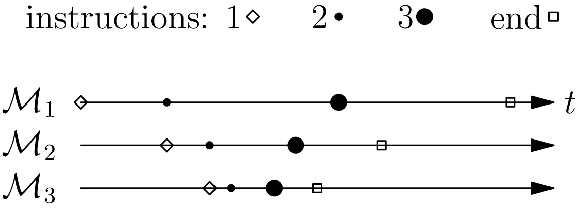
Figure 2: Starting time for each of instructions in machines ${\mathcal{M}}_{1}$, ${\mathcal{M}}_{2}$, ${\mathcal{M}}_{3}$.

IV The mechanical interpretation

Let us consider another variant of the inverted Thompson’s lamp paradox. Consider the mechanism ”mousetrap” depicted in Fig. 3. The mechanism consists of the beam on the spring. The beam in tension (vertical position) is fixed with a thread. When ball is tearing the tread, the beam latches horizontally and it does not let through another ball.

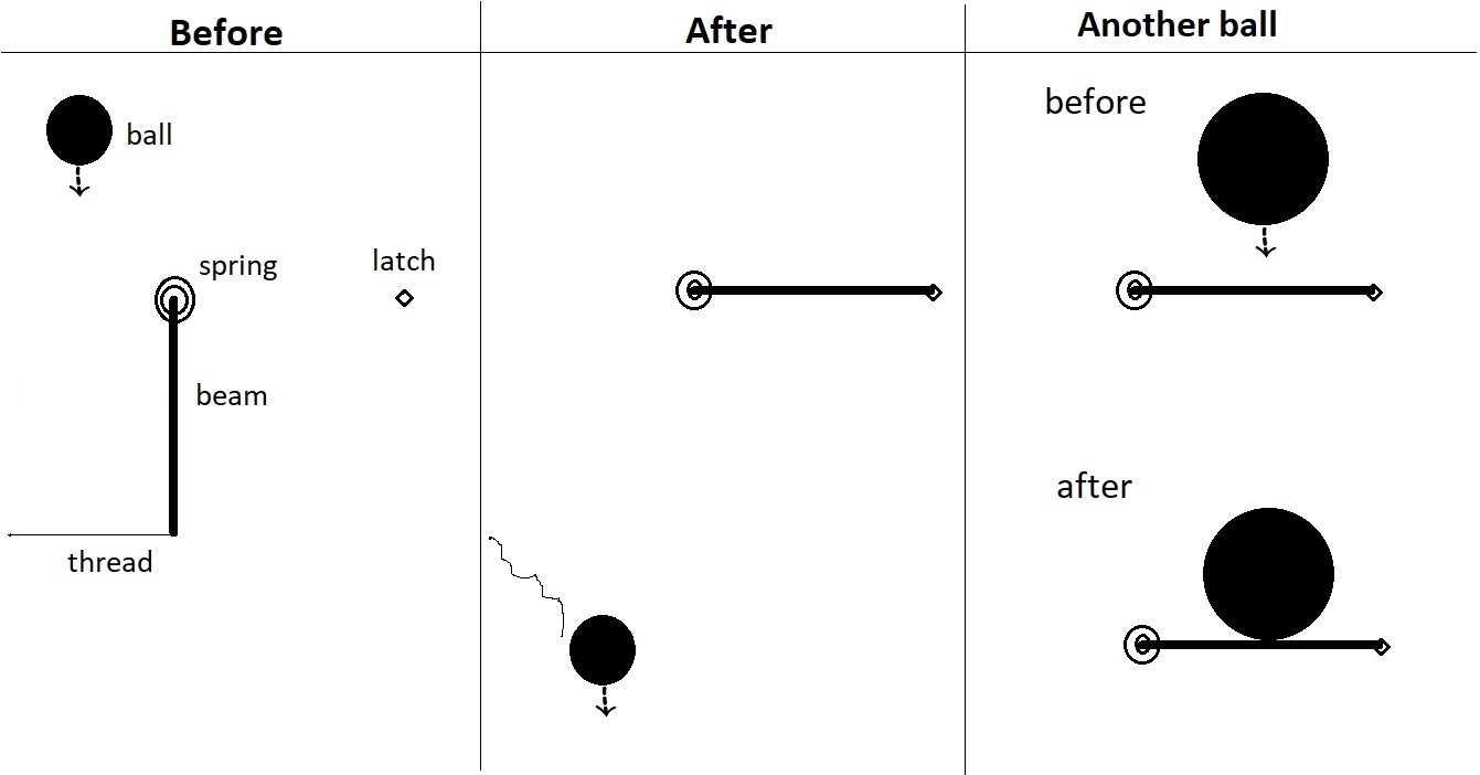
Figure 3: The structure of the finite mechanism.

Consider infinite number of the finite mechanisms depicted in Fig. 4. Each next finite mechanism is a small (half of the size) replica of the previous finite mechanism. To avoid various (e.g. centrifugal) effects, we can tune material properties of the spring and the beam of the next mechanism. We suppose also that there are infinite number of balls that move with a same constant velocity to the threads of the finite mechanisms. The size of each next ball is twice smaller than the size of the previous ball. The distances between the balls and the corresponding threads are chosen such that the smaller ball can tear the thread before the larger ball can reach the clipped horizontal beam corresponding to the smaller ball. Thus, the larger ball can not tear its thread since the beam is latched.

Note that any fixed constant value can be added to the distances between the balls and the threads. It is useful if we want that the smallest (limit) distance between the balls and the threads or beams is non-zero. Thus, there is a non-zero time interval between the start and the time when the balls reach the threads or latched beams.

The behavior of the infinite mechanism from Fig. 4 is indeterminate. We can not predict: will the largest beam be in a vertical or horizontal (latched) position after the balls fall down? The reason is the same as in the programm ”puzzle”. If the number of balls is a finite number, say $N$ then the largest beam is in a horizontal position for odd $N$ and in a vertical position for even $N$. But we can not say $N=\infty$ is even or odd number. Note that in our example we do not assume infinite masses, velocities, densities. So, the unpredictable infinite mechanism may well exist in a Newtonian Universe. Of course, such mechanism is not possible in our world because of the principles of quantum mechanics.

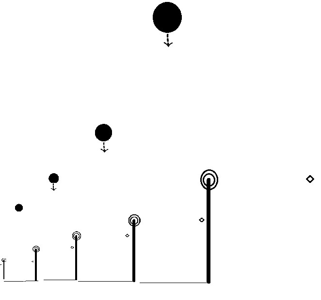
Figure 4: The infinite mechanism.

V Conclusion

Perhaps, any machine which uses the actual infinity is not free from Thompson-type paradoxes. Even physically reasonable assumptions may not be helpful. Probably, the main problem lies in our understanding of infinity. Nevertheless, a part of our mind can successfully develop infinite theories such as Peano arithmetic. Hence, there is a natural question which, however, can not be formulated rigorously: Is that part of our mind is an infinite machine and how it works?

References

- (1) J. Thompson, Tasks and supertasks, Analysis 15 (1954) 1–13.
- (2) G. S. Boolos, J. P. Burgess, R. C. Jeffrey, Computability and logic, Fifth edition, Princeton University, United States, 2007.
- (3) M. Hogarth, Predictability, computability, and spacetime, Cambridge University, 1996, phd thesis.
- (4) J. Earman, J. D. Norton, Infinite pains: The trouble with supertasks, in: A. Morton, S. P. Stich (Eds.), Benacerraf and his critics, Cambridge, MA: Blackwell, 1996, pp. 231–261.
- (5) E. B. Davies, Building infinite machines, Brit. J. Phil. Sci. 52 (2001) 671–682.
- (6) C. Wuthrich, A quantum-information-theoretic complement to a general-relativistic implementation of a beyond-Turing computer, Synthese 192 (2015) 1989–2008.
- (7) I. Nemeti, G. David, Relativistic computers and the Turing barrier, Appl. Math. Comput. 178 (2006) 118–142.
- (8) M. Stannett, Computing the appearance of physical reality, Appl. Math. Comput. 219 (2012) 54–62.
- (9) G. Falkovich, K. R. Sreenivasan, Lessons from hydrodynamic turbulence, Physics Today 59 (2006) 43–49.
- (10) P. Clark, S. Read, Hypertasks, Synthese 61 (1984) 387–390.
- (11) B. J. Copeland, Hypercomputation, Mind. Mach. 12 (2002) 461–502.
- (12) A. Hagar, A. Korolev, Quantum hypercomputability?, Mind. Mach. 16 (2006) 87–93.
- (13) P. Cotogno, A brief critique of pure hypercomputation, Mind. Mach. 19 (2009) 391–405.
- (14) A. Nayebi, Practical intractability: A critique of the hypercomputation movement, Mind. Mach. 24 (2014) 275–305.
- (15) S. Rummens, S. E. Cuypers, Determinism and the paradox of predictability, Erkenntnis 72 (2010) 233–249.