A Sharp Bound on the $s$-Energy and Its Applications to Averaging Systems

Abstract

The $s$-energy is a generating function of wide applicability in network-based dynamics. We derive an (essentially) optimal bound of $(3/\rho s)^{n-1}$ on the $s$-energy of an $n$-agent symmetric averaging system, for any positive real $s\leq 1$, where $\rho$ is a lower bound on the nonzero weights. This is done by introducing the new dynamics of twist systems. We show how to use the new bound on the $s$-energy to tighten the convergence rates of systems in opinion dynamics, flocking, and synchronization.

1 Introduction

Averaging dynamics over time-varying networks is a process commonly observed in many well-studied multiagent systems. It has been used to model swarming, polarization, synchronization, gossip processes, and consensus formation in distributed systems [2, 9, 10]. Because of a dearth of general convergence techniques, results in the area often rely on network connectivity assumptions. The $s$-energy is a powerful analytical tool that allows us to overcome these restrictions [4]. It provides a global parametrized measure of the “footprint” of the system over an infinite horizon. This stands in sharp contrast with the local arguments (spectral or Lyapunov-based) typically used to prove fixed-point attraction.

The main result of this paper is an optimal bound on the $s$-energy of symmetric averaging systems. The new bound is used to tighten the convergence rates of various multiagent systems in opinion dynamics, flocking, and self-synchronization of coupled oscillators [2, 4, 8, 11, 12, 14, 15, 16, 18, 20, 21, 22].

Before moving to the technical discussion, we illustrate the role of the $s$-energy with a toy system. Fix $\rho\in(0,1/2]$ and place $n$ agents at $x_{1},\ldots,x_{n}$ in $[0,1]$. Given any $\varepsilon>0$, for any integer $t>0$, pick two agents $i,j$ such that $x_{j}-x_{i}\geq\varepsilon$ (if any) and move them anywhere in the interval $[x_{i}+\delta,x_{j}-\delta]$, where $\delta=\rho(x_{j}-x_{i})$. Repeat this process as long as possible. Note the high nondeterminism of the dynamics: not only can we choose the pair of agents at each step, but we can move them anywhere we please within the specified interval. Despite this freedom, the process always terminates in $O\bigl{(}\frac{1}{\rho n}\log\frac{1}{\varepsilon}\bigr{)}^{n-1}$ steps, for any small enough $\varepsilon>0$, and the bound is tight. This result is a direct consequence of our new bound on the $s$-energy. The proof relies on a reduction to twist systems, a new type of multiagent dynamics that we define in the next section.

The $s$-energy.

Let $(g_{t})_{t=1}^{\infty}$ be an infinite sequence of graphs over a fixed vertex set $\{1,\ldots,n\}$. Each $g_{t}$ is embedded in $[0,1]$, meaning that its vertices (the “agents”) are represented by $n$ real numbers between 0 and 1. Let $\mu_{1},\ldots,\mu_{k}$ denote the lengths of the intervals formed by the union of the embedded edges of $g_{t}$, and put $\ell_{t}=\mu_{1}^{s}+\cdots+\mu_{k}^{s}$, for real or complex $s$. The $s$-energy ${\mathcal{E}}(s)$ of the system is defined as the infinite sum $\sum_{t>0}\ell_{t}$. Because the $s$-energy follows an obvious scaling law, we note that embedding the graphs in the unit interval is not restrictive.

Averaging systems.

In a (symmetric) averaging system, $g_{t}$ is undirected and supplied with self-loops at the vertices. To simplify the notation, we fix $t\in\mathbb{Z}^{+}$ and denote by $x_{i}$ and $y_{i}$ the positions of vertex $i$ at times $t$ and $t+1$, respectively. Vertices are labeled so that $x_{1}\leq\cdots\leq x_{n}$. For each $i\in\{1,\ldots,n\}$, write $r(i)=\max\{j\,|\,(i,j)\in g_{t}\}$ and $l(i)=\min\{j\,|\,(i,j)\in g_{t}\}$. Fix $\rho\in(0,1/2]$. The move of vertex $i$ from $x_{i}$ to $y_{i}$ is subject to

$$x_{l(i)}+\delta_{i}\leq y_{i}\leq x_{r(i)}-\delta_{i},$$ (1)

where $\delta_{i}=\rho(x_{r(i)}-x_{l(i)})$. In other words, vertex $i$ can move anywhere within the interval covered by its incident edges, but not too close to the endpoints. If $\rho=0$, convergence is clearly impossible to ensure since $i$ can easily oscillate periodically between two fixed vertices. We emphasize the high nondeterminism of the process: $g_{t}$ is arbitrary and so is the motion of $i$ within its allotted interval.

The results.

Although the $0$-energy is typically unbounded, it may come as a surprise that ${\mathcal{E}}(s)$ is always finite for any $s>0$ [4]. In particular, the case $s=1$ shows that it takes only a finite amount of ink to draw the infinite sequence of graphs $g_{t}$. We state the main result of this article, and prove it in §3:

Theorem 1.1

$\!\!\!.\,\,$ The $s$-energy satisfies ${\mathcal{E}}(s)\leq(3/\rho s)^{n-1}$, for any $0<\rho\leq 1/2$ and $0<s\leq 1$.

We prove in §5.A that the bound $O(1/\rho s)^{n-1}$ is optimal for $s=O\bigl{(}1/\log\frac{1}{\rho}\bigr{)}$ and $\rho\leq 1/3$. These are the conditions we encounter in practice, which is why we are able to provide tight bounds for all the applications discussed in this work. For $s=1$, a quasi-optimal lower bound of $\Omega(1/\rho)^{\lfloor n/2\rfloor}$ is already known [4]. Theorem 1.1 lowers the previous upper bound of $(1/s)^{n-1}(1/\rho)^{n^{2}+O(1)}$ [4].

The $s$-energy helps us bound the convergence rates of averaging network systems in full generality. To our knowledge, no other current technique can prove these results. The power of the $s$-energy is that it makes no connectivity requirements about the underlying dynamic networks. We use it typically to bound the communication count $\mathcal{C}_{\varepsilon}$, which is defined as the maximum number of steps $t$ such that $g_{t}$ has at least one edge of length $\varepsilon>0$ or higher. From the inequality $\mathcal{C}_{\varepsilon}\leq\varepsilon^{-s}{\mathcal{E}}(s)$, setting $s=1/\log\frac{1}{\varepsilon}$ and $s=n/\log\frac{1}{\varepsilon}$ in Theorem 1.1 yields:

Theorem 1.2

$\!\!\!.\,\,$ The communication count satisfies $\mathcal{C}_{\varepsilon}=O\Bigl{(}\frac{1}{\rho}\log\frac{1}{\varepsilon}\Bigr{)}^{n-1}$ for any $2^{-n}\leq\varepsilon\leq 1/2$, and $\mathcal{C}_{\varepsilon}=O\Bigl{(}\frac{1}{\rho n}\log\frac{1}{\varepsilon}\Bigr{)}^{n-1}$ for $0<\varepsilon<2^{-n}$.

This lowers the previous upper bound of $(1/\rho)^{n^{2}+O(1)}(\log 1/\varepsilon)^{n-1}$ [4]. We prove in §5.B that the new bound is optimal for any positive $\varepsilon\leq\rho^{2n}$ and $\rho\leq 1/3$. We close this introduction with a few remarks about the results and their context:

1. The results extend to a large family of asymmetric averaging systems. Indeed, Theorems 1.1 and 1.2 hold for any infinite sequence of cut-balanced digraphs $g_{t}$: recall that a directed graph is said to be cut-balanced if its weakly connected components are also strongly connected.

2. The polylogarithmic factor $\bigl{(}\log 1/\varepsilon\bigr{)}^{n-1}$ in the convergence rate of Theorem 1.2 is a distinctive feature of time-varying network-based dynamics. Markov chains, for example, have convergence rates proportional to $\log 1/\varepsilon$.

3. Our definition of the $s$-energy differs slightly from the original formulation [4], which introduced the total $s$-energy as $\sum_{t>0}\sum_{(i,j)\in g_{t}}d_{ij}(t)^{s}$, where $d_{ij}(t)$ is the distance between the vertices $i,j$ in the embedding of $g_{t}$. Up to a correction factor of at most $\binom{n}{2}$, our bounds apply to the total $s$-energy as well.

4. As noted in [7], the $s$-energy can be interpreted as a generalized Dirichlet series or, alternatively, as a partition function with $s$ as the inverse temperature. Both interpretations have their own benefits, such as highlighting the lossless encoding properties of the $s$-energy or the usefulness of Legendre-transform arguments with the relevant thermodynamical quantities.

2 Twist Systems

We reduce averaging systems to a simpler kind of dynamics where agents keep the same ordering at all time. In a twist system, $n$ points move within $[0,1]$ at discrete time steps. As before, we fix $t\in\mathbb{Z}^{+}$ and describe the motion of each point $x_{i}$ at time $t$ to its next position $y_{i}$ at time $t+1$. Unlike the averaging kind, twist systems preserve order; that is, assuming that $x_{1}\leq\cdots\leq x_{n}$, then $y_{1}\leq\cdots\leq y_{n}$. To describe the motion from $t$ to $t+1$, we choose two integers $1\leq u<v\leq n$ and, for any $i$ ($u\leq i\leq v$), we define the twist of $x_{i}$ as the interval within $[x_{u},x_{v}]$ defined by

$$\tau_{i}=\bigl{[}x_{u}+\rho(x_{\min\{i+1,v\}}-x_{u}),x_{v}-\rho(x_{v}-x_{\max\{i-1,u\}})\bigr{]}.$$ (2)

Fixing $\rho\in(0,1/2]$ ensures that all the twists are well-defined. The only constraints on the dynamics are: (i) $y_{1}\leq\cdots\leq y_{n}$; and (ii) $y_{i}\in\tau_{i}$ for any $u\leq i\leq v$, and $y_{i}=x_{i}$ otherwise.

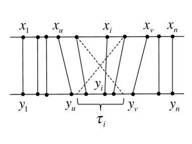
Figure 1: The interval $\tau_{i}$ extends from a distance $\rho(x_{i+1}-x_{u})$ to the right of $x_{u}$ to a distance $\rho(x_{v}-x_{i-1})$ to the left of $x_{v}$: it thus twists $[x_{i-1},x_{i+1}]$ into the allowed interval for $y_{i}$.

Observe that conditions (i,ii) are always feasible: for example, we can choose $y_{i}$ to be the leftmost point in $\tau_{i}$; of course, there is no need to do so and the expressive power of twist systems comes from the freedom they offer. Like their averaging counterparts, such systems are highly nondeterministic: at each step $t$, both the choice of $u,v$ and the motion of the points are entirely arbitrary within the constraints (i,ii). Writing $\ell_{t}=(x_{v}-x_{u})^{s}$, we define the $s$-energy of the twist system as ${\mathcal{E}}(s)=\sum_{t>0}\ell_{t}$. The next result justifies the introduction of twist systems.

Theorem 2.1

$\!\!\!.\,\,$ Any averaging system can be viewed as a twist system with the same parameter $\rho$ and the same $s$-energy.

Proof. Referring to our previous notation, recall that $\mu_{1},\ldots,\mu_{k}$ denote the lengths of the intervals $I_{j}$ formed by the union of the edge embeddings of $g_{t}$. We subdivide the time interval from $t$ to $t+1$ into $k$ time windows and, for $j=1,\ldots,k$, we process the motion within $I_{j}$ during the $j$-th window while keeping the other vertices fixed. All windows are treated similarly, so it suffices to explain the case $k=1$. Let $x_{i}$ (resp. $x_{i}^{\prime}$) be the position of vertex $i$ at time $t$ (resp. $t+1$) and let $y_{1}\leq\cdots\leq y_{n}$ be the sequence of $x_{i}^{\prime}$ sorted in nondecreasing order. Let $x_{u},\ldots,x_{v}$ denote the positions within $I_{1}$; we may assume that $u<v$. The other vertices are kept fixed, so we have $y_{i}=x_{i}$ for $i<u$ or $i>v$. To show that the transition from $x_{i}$ to $y_{i}$ meets the conditions of a twist system, we need to prove that $y_{i}\in\tau_{i}$ for any $i$ between $u$ and $v$. By the symmetry of (2), it suffices to show that, for $u\leq i\leq v$,

$$y_{i}\leq x_{v}-\rho(x_{v}-x_{\max\{i-1,u\}}).$$ (3)

Assume that $u<i\leq v$ and let $\bar{x}_{j}$ be shorthand for $\rho x_{j}+(1-\rho)x_{v}$. The entire interval $I_{1}$ is covered by edges of $g_{t}$, so there must be at least one edge $(a,b)$ that covers $[x_{i-1},x_{i}]$, ie, $b<i\leq a$. By (1), $x_{a}^{\prime}\leq\rho x_{l(a)}+(1-\rho)x_{r(a)}$, with $l(a)\leq b<i$ and $r(a)\leq v$; hence $x_{a}^{\prime}\leq\bar{x}_{i-1}$. It also follows from (1) and the presence of self-loops that $x_{j}^{\prime}\leq\rho x_{l(j)}+(1-\rho)x_{r(j)}\leq\bar{x}_{i-1}$ for any $j$ ($u\leq j<i$); also $x_{j}^{\prime}=x_{j}\leq\bar{x}_{i-1}$ for $j<u$. Putting it all together, this proves the existence of at least $i$ indices $l\leq v$ such that $x_{l}^{\prime}\leq\bar{x}_{i-1}$. It follows that $y_{i}\leq\bar{x}_{i-1}$; hence (3) for $u<i\leq v$. To complete the proof of (3), we note that the case $i=u$ follows from $y_{u}\leq y_{u+1}$. The case $k>1$ is handled by repeating the previous analysis for each interval $I_{j}$. The $s$-energy contributed by one step of the averaging system matches the energetic contribution of the $k$ substeps of the twist system. $\Box$

3 Bounding the $s$-Energy

The proof of Theorem 1.1 is unusual in the context of dynamics because it is algorithmic: it consists of a set of trading rules that allows money to be injected into the system and exchanged among the vertices to meet their needs. As the transactions take place, money is spent to pay for the $s$-energy expended along the way. If all of the energy can be accounted for in this manner, then the amount of money injected in the system is an upper bound on $\mathcal{E}(s)$. In our earlier work [4], we were able to pursue this approach only for the case $s=1$. We show here how to extend it to all $s\in(0,1]$. The idea was to supply each vertex with its own credit account and then let them trade credits to pay for the $s$-energy incrementally. This strategy does not work here because of its inability to cope with all the scales present in the system. The remedy is to supply each pair of vertices with their own account. Only then are we able to accommodate all scales at once. By appealing to Theorem 2.1, we may substitute twist systems for averaging systems. We focus the analysis on the transition at time $t$ from $x_{1}\leq\cdots\leq x_{n}$ to $y_{1}\leq\cdots\leq y_{n}$. Our only assumption is that, for some $u,v$ ($1\leq u<v\leq n$), we have $y_{i}\in\tau_{i}$ for any $u\leq i\leq v$, and $y_{i}=x_{i}$ otherwise.

For each pair $(i,j)$ such that $1\leq i<j\leq n$, we maintain an account $B_{i,j}$ consisting of $(x_{j}-x_{i})^{s}A^{j-i}$ credits, where $A\!:=2/\rho s$ and one credit is used to pay for a single unit of $s$-energy. (Amounts paid need not be integers.) We show that updating each $B_{i,j}$ at time $t$ to $B_{i,j}^{\prime}$ at time $t+1$ leaves us with enough unused money to pay for the $s$-energy $(x_{v}-x_{u})^{s}$ released at that step. No new money is needed past the initial injection at time 1, so the $s$-energy is at most the sum of all the $B_{i,j}$’s at the beginning: ${\mathcal{E}}(s)\leq\sum_{i<j}A^{j-i}<\bigl{(}\frac{A}{A-1}\bigr{)}^{2}A^{n-1}<2(2/\rho s)^{n-1}$, for $n>2$. For $n=2$, ${\mathcal{E}}(s)\leq A$, hence Theorem 1.1. We begin with a few words of intuition:

• We update $B_{i,j}$ to $B^{\prime}_{i,j}$ by considering the pairs $(i,j)$ in descending order of $j-i$, starting with $(1,n)$. In general, the update for $(i,j)$ will rely on money released by the pairs $(i-1,j)$ and $(i,j+1)$, whose accounts will have already been updated. In turn, the pair $(i,j)$ will then be expected to provide money to both $(i,j-1)$ and $(i+1,j)$: the donation will be made in two equal amounts.

• How much money should $(i,j)$ receive from its donors. For the sake of this informal discussion, let us focus on the case $u\leq i<j\leq v$. The account $B_{i,j}$ should receive enough to grow to $(x_{v}-x_{u})^{s}A^{j-i}$. This typically exceeds its balance of $(x_{j}-x_{i})^{s}A^{j-i}$ at time $t$, so an infusion of money is required. Of course, the amount actually needed for $B^{\prime}_{i,j}$ is only $(y_{j}-y_{i})^{s}A^{j-i}$, so this in turn frees $\bigl{(}(x_{v}-x_{u})^{s}-(y_{j}-y_{i})^{s}\bigr{)}A^{j-i}\geq 0$, which can be then passed on to $(i,j-1)$ and $(i+1,j)$.

• We pay for the energetic contribution at time $t$ by spending the leftover money from the update for $(u,u+1)$, which we show to be at least $(x_{v}-x_{u})^{s}$, as required.

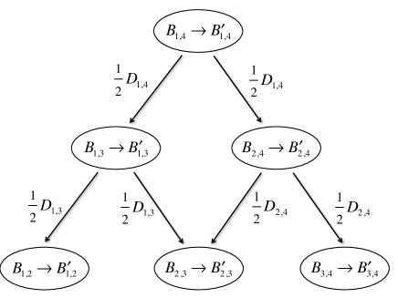
Figure 2: Updating $B_{1,4}$ to its new value of $B^{\prime}_{1,4}$ releases $D_{1,4}$ credits, which are passed on evenly to the pairs $(1,3)$ and $(2,4)$. With this scheme in place, updating $B_{2,3}$ to $B^{\prime}_{2,3}$ can make use of $C_{2,3}=\frac{1}{2}(D_{1,3}+D_{2,4})$ credits.

Proof of Theorem 1.1. We update $B_{i,j}$ by using $C_{i,j}$ credits supplied by the accounts $B_{i-1,j}$ and $B_{i,j+1}$. We show how this produces a leftover $D_{i,j}$, which can then be donated to $(i+1,j)$ and $(i,j-1)$ in equal amounts. Here are the details: for all $1\leq i<j\leq n$ in descending order of $j-i=n-1,\ldots,1$, apply the following assignments (Fig.2):

$$\begin{cases}\,C_{i,j}\leftarrow\,\frac{1}{2}(D_{i-1,j}+D_{i,j+1})\\ \,D_{i,j}\leftarrow\,B_{i,j}+C_{i,j}-B^{\prime}_{i,j},\end{cases}$$ (4)

where $B_{i,j}=(x_{j}-x_{i})^{s}A^{j-i}$, $B^{\prime}_{i,j}=(y_{j}-y_{i})^{s}A^{j-i}$, and $D_{i,j}=0$ if $i<1$ or $j>n$. The assignments denote transfers of money. This explains the factor of $1/2$, which keeps the money pool conserved: for example, one half of $D_{i,j}$ goes to $(i,j-1)$ and the other half to $(i+1,j)$. The soundness of the trading scheme rests entirely on the claimed nonnegativity of all the donations $D_{i,j}$. For any $i\in\{1,\ldots,n\}$, define $u(i)=u$ and $v(i)=v$ if $u\leq i\leq v$; and set $u(i)=v(i)=i$ otherwise. We prove by induction on $j-i>0$ that, for $1\leq i<j\leq n$,

$$\,B_{i,j}+C_{i,j}\geq(x_{v(j)}-x_{u(i)})^{s}A^{j-i}$$ (5)

$$\,D_{i,j}\geq 0.$$ (6)

The next inequality, which follows from $dz^{s}/dz\geq s$ for $s,z\in(0,1]$, will prove useful in establishing (5, 6):

$$1-(1-x)^{s}\geq sx\hskip 8.5359pt\text{for any $s,x\in[0,1]$.}$$ (7)

$\bullet$ Case $u\leq i<j\leq v$. By affine invariance, we can always assume that $x_{u}=x_{v}-1=0$. We begin with the case $u<i<j\leq v$ and observe that $v(j)=v$ and $u(i-1)=u(i)=u$. Because $y_{i-1}\in\tau_{i-1}$, we have $y_{i-1}\geq\rho x_{i}$. Using (7), we find that

$$\begin{split}D_{i-1,j}&=B_{i-1,j}+C_{i-1,j}-B^{\prime}_{i-1,j}\geq\bigl{(}(x_{v(j)}-x_{u(i-1)})^{s}-(y_{j}-y_{i-1})^{s}\bigr{)}A^{j+1-i}\\ &\geq\bigl{(}1-(1-\rho x_{i})^{s}\bigr{)}A^{j+1-i}\geq\rho sx_{i}A^{j+1-i}.\end{split}$$ (8)

If $i=u$, we have $x_{i}=0$, hence (8) merely expresses nonnegativity, which holds inductively. We conclude that (8) obtains for any $u\leq i<j\leq v$. Likewise, by symmetry, $D_{i,j+1}\geq\rho s(1-x_{j})A^{j+1-i}$. It follows from (4) that $C_{i,j}\geq\frac{1}{2}\rho s\bigl{(}1-(x_{j}-x_{i})\bigr{)}A^{j+1-i}\geq\bigl{(}1-(x_{j}-x_{i})^{s}\bigr{)}A^{j-i}$; therefore,

$$B_{i,j}+C_{i,j}\geq(x_{j}-x_{i})^{s}A^{j-i}+\bigl{(}1-(x_{j}-x_{i})^{s}\bigr{)}A^{j-i}=A^{j-i}=(x_{v(j)}-x_{u(i)})^{s}A^{j-i},$$

which establishes (5). Since $x_{u(i)}=x_{u}\leq y_{i}\leq y_{j}\leq x_{v}=x_{v(j)}$, this also proves that

$$D_{i,j}=B_{i,j}+C_{i,j}-B^{\prime}_{i,j}\geq A^{j-i}-(y_{j}-y_{i})^{s}A^{j-i}\geq 0;$$

hence (6).

$\bullet$ Case $i<u\leq j\leq v$. This time, we set $x_{i}=0$ and $x_{v}=1$ and note that $u(i)=i$ and $v(j)=v$. We begin with the case $j<v$, which implies that $v(j+1)=v$. Using (4, 5), $y_{i}=x_{i}$, $y_{j+1}\in\tau_{j+1}$, and (7) in this order, we find that

$$\begin{split}D_{i,j+1}&=B_{i,j+1}+C_{i,j+1}-B^{\prime}_{i,j+1}\geq\bigl{(}(x_{v(j+1)}-x_{u(i)})^{s}-(y_{j+1}-x_{i})^{s}\bigr{)}A^{j+1-i}\\ &\geq\bigl{(}1-(1-\rho(1-x_{j}))^{s}\bigr{)}A^{j+1-i}\geq\rho s(1-x_{j})A^{j+1-i}\geq(1-x_{j})A^{j-i}.\end{split}$$ (9)

Again, by induction, $D_{i-1,j}\geq 0$; therefore, by (4),

$$B_{i,j}+C_{i,j}\geq B_{i,j}+\hbox{$\frac{1}{2}$}D_{i,j+1}\geq\bigl{(}x_{j}^{s}+(1-x_{j})\bigr{)}A^{j-i}\geq A^{j-i}=(x_{v(j)}-x_{u(i)})^{s}A^{j-i};$$

hence (5). For the case $j=v$, again note that the lower bounds on $D_{i-1,j}$ and $D_{i,j+1}$ we just used still hold, and thus so does (5) for all $i<u\leq j\leq v$. Finally, $y_{j}\leq x_{v}$; hence $x_{u(i)}=x_{i}=y_{i}\leq y_{j}\leq x_{v}=x_{v(j)}$, and (6) follows from (4, 5).

The case $u\leq i\leq v<j$ is the mirror image of the last one while the remaining three cases are trivial and require no account updates. We pay for the $s$-energy contribution at time $t$ by tapping into $D_{u,u+1}$, which is unused. For this to work, it suffices to show that $D_{u,u+1}\geq(x_{v}-x_{u})^{s}$. We have $y_{i}\in\tau_{i}$ ($i=u,u+1$); hence

$$\begin{split}y_{u+1}-y_{u}&\leq x_{v}-\rho(x_{v}-x_{u})-(x_{u}+\rho(x_{u+1}-x_{u}))\\ &\leq\rho(x_{u}-x_{u+1})+(1-\rho)(x_{v}-x_{u})\leq(1-\rho)(x_{v}-x_{u}).\end{split}$$

Thus, it follows from (4, 5, 7), together with $u(u)=u$ and $v(u+1)=v$, that

$$\begin{split}D_{u,u+1}&=B_{u,u+1}+C_{u,u+1}-B^{\prime}_{u,u+1}\geq A(x_{v(u+1)}-x_{u(u)})^{s}-A(y_{u+1}-y_{u})^{s}\\ &\geq\bigl{(}1-(1-\rho)^{s}\bigr{)}A(x_{v}-x_{u})^{s}\geq\rho sA(x_{v}-x_{u})^{s}\geq(x_{v}-x_{u})^{s}.\end{split}$$

This completes the proof of Theorem 1.1 for twist systems. By Theorem 2.1, this also implies the same upper bound for averaging systems. $\Box$

4 Applications

A number of known convergence rates for various averaging systems can be sharpened by appealing to Theorems 1.1 and 1.2. We give a few examples below.

4.1 Asymmetric averaging systems

Symmetric averaging systems have been widely used to model backward products of the form $(A_{t}\cdots A_{1}x)_{t>0}$, where each $A_{k}$ is a type-symmetric stochastic matrix with positive diagonal and nonzero entries at least $\rho>0$ [3, 9, 12, 14, 16, 18]. In other words, $A_{k}$ is the matrix of a lazy random walk in an undirected graph $g_{k}$ with a lower bound of $\rho$ on the nonzero probabilities. A close examination of the proof of Theorem 2.1 shows that the graphs $g_{t}$ may be directed as long as the vertices still have self-loops, and, for each $i=u+1,\ldots,v$, there exist edges “hovering” over $i$ from both sides, ie, $(a,b)$ and $(b^{\prime},a^{\prime})$, with $a,a^{\prime}<i\leq b,b^{\prime}$. We note that this property holds if each directed graph $g_{t}$ is cut-balanced. This gives us a strict generalization of Theorems 1.1 and 1.2 for asymmetric averaging systems whose sequences of digraphs are cut-balanced. This goes beyond the convergence of these systems, which was established in [13].

4.2 Opinion dynamics

There has been considerable attention given to consensus formation in social dynamics [9, 10, 11]. Given a set of agents in high-dimensional space, where coordinates model opinions, one imagines that at each step a subset of them come into contact and, through a process of deliberation, adjust their opinions toward agreement. Will such a process converge to consensus, polarization, a mixture of both, or not at all? Mathematically, the agents are represented by their position in $d$-dimensional space: $x_{1},\ldots,x_{n}$ in $[0,1]^{d}$. We fix $0<\alpha\leq 1$ and iterate on the following process forever: (1) choose an arbitrary nonempty subset of the agents and move them anywhere inside the box $(1-\alpha)B+\alpha c$, where $B$ is the smallest (axis-parallel) box enclosing the chosen agents and $c$ is the center of $B$; (2) repeat. Intuitively, one “squeezes” the subset of agents together a little.

Theorem 4.1

$\!\!\!.\,\,$ For any positive $\varepsilon\leq 2^{-dn}$, at all but $O\bigl{(}\frac{1}{d\alpha n}\log\frac{1}{\varepsilon}\bigr{)}^{n-1}$ time steps, the smallest box enclosing the chosen agents has volume less than $\varepsilon$.

Proof. We set up a symmetric averaging system as follows: $g_{t}$ consists of $n$ self-loops, together with the complete graph joining the agents of the chosen subset; along each axis, the dynamics obeys (1) with parameter $\rho=\alpha/2$. Let $\ell_{t}(j)$ be the length of the graph’s projection onto the $j$-th axis. By Theorem 1.1, we know that, for any $0<r\leq 1$, $\sum_{t>0}\ell_{t}(j)^{r}\leq(6/\alpha r)^{n-1}$. Let $V_{t}$ be the volume of the smallest box enclosing the agents picked at time $t$. By the generalized Hölder’s inequality, for $0<s\leq 1/d$,

$$\sum_{t>0}V_{t}^{s}=\sum_{t>0}\prod_{j=1}^{d}\ell_{t}(j)^{s}\leq\prod_{j=1}^{d}\,\Bigl{(}\sum_{t>0}\ell_{t}(j)^{ds}\Bigr{)}^{1/d}\leq(6/d\alpha s)^{n-1}.$$

Set $s=n/\log\frac{1}{\varepsilon}$ and use Markov’s inequality to complete the proof. $\Box$

4.3 Flocking

Many models of bird flocking have been developed over the years and used to great effect in CGI for film and animation. Their mathematical analysis has lagged behind, however. In a simple, popular model tracing its roots back to Cucker & Smale, Vicsek, and ultimately Reynolds, a group of $n$ birds is represented by two $n$-by-$3$ matrices $\mathbf{x}(t)$ and $\mathbf{v}(t)$, where the $i$-th rows encode the location and velocity in $\mathbb{R}^{3}$ of the $i$-th bird, respectively [8, 14, 22]. The dynamics obeys the relations

$$\begin{cases}\,\,\mathbf{x}(t)=\mathbf{x}(t-1)+v(t)\\ \,\,\mathbf{v}(t+1)=P(t)\,\mathbf{x}(t),\end{cases}$$

where $P(t)$ is an $n$-by-$n$ stochastic matrix whose entry $(i,j)$ is positive if and only if birds $i$ and $j$ are within a fixed distance $R$ of each other. All entries are rationals over $O(\log n)$ bits. A tight bound on the convergence of the dynamical system was established in [5, 6]: it was shown that steady state is always reached within a number of steps equal to a tower-of-twos of height proportional to $\log n$; even more amazing, this bound is optimal. The lead-up to steady-state consists of two phases: fragmentation and aggregation. The latter can feature only the merging of flocks while the (much shorter) fragmentation phase can witness the repeated formation and breakup of flocks. Technically, a flock is defined as the birds in a given connected component of the network joining any two birds within distance $R$. It has been shown that the total number of network switches (ie, the number of steps where the communication network changes) is $n^{O(n^{2})}$. We improve this bound to $n^{O(n)}$ by using the $s$-energy. It was demonstrated in [5] (page 21:7) that the number of network switches is bounded by the communication count $C_{\varepsilon}$, for $\varepsilon\geq n^{-bn^{2}}$, $\rho\geq n^{-c}$ and constant $b,c>0$. Our claim follows from Theorem 1.2. $\Box$

4.4 Self-synchronizing oscillators

The self-organized synchronization of coupled oscillators is a well-known phenomenon in physics and biology: it is observed in circadian neurons, firing fireflies, yeast cell suspensions, cardiac pacemaker cells, power plant grids, and even musical composition (eg, Ligeti’s poème symphonique). In the discrete Kuramoto model studied in [17, 18, 19], all oscillators share the same natural frequency and the phase of the $i$-th one obeys the recurrence:

$$\theta_{i}(t+1)=\theta_{i}(t)+\frac{K\Delta T}{|n_{i}(t)|}\sum_{j\in n_{i}(t)}\sin\bigl{(}\theta_{j}(t)-\theta_{i}(t)\bigr{)},$$

where $n_{i}(t)$ is the set of vertices adjacent to $i$ in $g_{t}$ (which includes $i$). Following [18], we assume that all $n$ phases start in the same open half-circle, which we can express as $\alpha-\pi/2\leq\theta_{i}(0)\leq\pi/2$, for some arbitrarily small positive constant $\alpha$. We find that $\sin(\theta_{j}(0)-\theta_{i}(0))=a_{ij}\bigl{(}\theta_{j}(0)-\theta_{i}(0)\bigr{)}$, where $c\alpha\leq a_{ij}\leq 1$, for constant $c>0$. This condition holds for all $t$ since averaging keeps the phases in the same open half-circle. The dynamics is that of a symmetric averaging system provided that we pick $\rho$ small enough so that $b\rho n/\alpha\leq K\Delta T\leq 1$, for a suitable constant $b>0$. By Theorem 1.2, for any $\varepsilon\leq 2^{-n}$, the number of steps where two oscillators are joined by an edge while their phases are off by $\varepsilon$ or more is $O\bigl{(}\frac{1}{\alpha K\Delta T}\log\frac{1}{\varepsilon}\bigr{)}^{n-1}$.

5 The Lower Bound Proofs

A. We prove that the bound $O(1/\rho s)^{n-1}$ from Theorem 1.1 is optimal for $s=O\bigl{(}1/\log\frac{1}{\rho}\bigr{)}$ and $\rho\leq 1/3$. A lower bound construction from [4] (page 1703) describes a system whose $n$-agent $s$-energy satisfies the recurrence $\mathcal{E}_{n}\geq\rho^{s}\mathcal{E}_{n-1}+(1-2\rho)^{s}\mathcal{E}_{n}+1$ for $n>1$; hence, for positive constant $b$, $\mathcal{E}_{2}\geq b/\rho s$ and $\mathcal{E}_{n}\geq(b\rho^{s-1}/s)\mathcal{E}_{n-1}$ for $n>2$. This shows that $\mathcal{E}_{n}\geq(b/\rho s)^{n-1}\rho^{s(n-2)}=\Omega(1/\rho s)^{n-1}$, for $s=O\bigl{(}1/\log\frac{1}{\rho}\bigr{)}$, as claimed. $\Box$

B. We prove that $\mathcal{C}_{\varepsilon}=\Omega\Bigl{(}\frac{1}{\rho n}\log\frac{1}{\varepsilon}\Bigr{)}^{n-1}$, for any positive $\varepsilon\leq\rho^{2n}$ and $\rho\leq 1/3$. Note that $\rho$ must be bounded away from $1/2$ (we choose $1/3$ for convenience): indeed, in the case of two vertices at distance 1 joined by an edge, we have the trivial bound $C_{\varepsilon}=1$ for $\rho=1/2$. The proof revisits an earlier construction [4] and modify its analysis to fit our purposes. If $n>1$, the $n$ vertices of $g_{1}$ are positioned at 0, except for $x_{n}=1$. Besides the self-loops, the graph $g_{1}$ has the single edge $(n-1,n)$. At time 2, the vertices are all at $0$ except for $x_{n-1}=\rho$ and $x_{n}=1-\rho$. The first $n-1$ vertices form a system that stays in place if $n=2$ and, otherwise, proceeds recursively within $[0,\rho]$ until it converges to the fixed point $\rho/(n-1)$: this value is derived from the fact that each step keeps the mass center invariant. After convergence of the vertices labeled $1$ through $n-1$, the $n$-vertex system repeats the previous construction within $[\rho/(n-1),1-\rho]$. Let $C(n,\varepsilon)$ denote the communication count for $n$ agents: we have $C(n,\varepsilon)=0$ if $n=1$ or $\varepsilon>1$; else

$$C(n,\varepsilon)\geq 1+C\,\biggl{(}\,n-1,\frac{\varepsilon}{\rho}\,\biggr{)}+C\,\biggl{(}\,n,\frac{\varepsilon}{1-\rho n/(n-1)}\,\biggr{)}\,.$$ (10)

By expanding the recurrence and using monotonicity,

$$C(n,\varepsilon)\geq k+k\,C\,\biggl{(}\,n-1,\frac{\varepsilon}{\rho(1-2\rho)^{k-1}}\,\biggr{)}\,\,,\hskip 8.5359pt\text{for}\,\,\,k=\biggl{\lceil}\frac{(\log\varepsilon)/n-\log\rho}{2\log(1-2\rho)}\biggr{\rceil}.$$ (11)

Assume now that $\varepsilon\leq\rho^{2n}$. From our choice of $k$, we easily verify that

$$\rho(1-2\rho)^{k-1}\geq\varepsilon^{1/n}\,.$$ (12)

The recurrence (11) requires that $\varepsilon/\bigl{(}\rho(1-2\rho)^{k-1}\bigr{)}<1$, which follows from (12). Since $\varepsilon^{1/2n}\leq\rho\leq 1/3$, we have $k\geq\frac{b}{\rho n}\log\frac{1}{\varepsilon}$, for constant $b>0$. It follows that $C(2,\varepsilon)=\Omega(\frac{1}{\rho}\log\frac{1}{\varepsilon})$ and, for $n>2$, by (12),

$$C(n,\varepsilon)\geq\biggl{(}\,\frac{b}{\rho n}\log\frac{1}{\varepsilon}\,\biggr{)}\,\,C\Bigl{(}n-1,\varepsilon^{1-1/n}\Bigr{)}.$$

We verify that the condition $\varepsilon\leq\rho^{2n}$ holds recursively: $\varepsilon^{1-1/n}\leq\rho^{2(n-1)}$. By induction, it follows that $C(n,\varepsilon)\geq\Omega\Bigl{(}\frac{1}{\rho n}\log\frac{1}{\varepsilon}\Bigr{)}^{n-1}$, as desired. $\Box$

References

- [1]
- [2] Bullo, F., Cortés, J., Martinez, S., Distributed Control of Robotic Networks, Applied Mathematics Series, Princeton University Press, 2009.
- [3] Cao, M., Spielman, D.A. Morse, A.S. A lower bound on convergence of a distributed network consensus algorithm, 44th IEEE Conference on Decision and Control, and the European Control Conference, Seville, Spain (2005), 2356–2361.
- [4] Chazelle, B. The total -energy of a multiagent system, SIAM J. Control Optim. 49 (2011), 1680–1706.
- [5] Chazelle, B. The convergence of bird flocking, Journal ACM 61 (2014), 21:1–35.
- [6] Chazelle, B. How many bits can a flock of birds compute?, Theory of Computing 10 (2014), 421–451.
- [7] Chazelle, B. An algorithmic approach to collective behavior, Journal of Statistical Physics 158 (2015), 514–548.
- [8] Cucker, F., Smale, S. Emergent behavior in flocks, IEEE Transactions on Automatic Control 52 (2007), 852–862.
- [9] Fagnani, F., Frasca, P. Introduction to Averaging Dynamics over Networks, Lecture Notes in Control and Information Sciences 472, Springer, 2018.
- [10] Fortunato S. On the consensus threshold for the opinion dynamics of Krause-Hegselmann, International Journal of Modern Physics C, 16, 2 (2005), 259–270.
- [11] Hegselmann, R., Krause, U. Opinion dynamics and bounded confidence models, analysis, and simulation, J. Artificial Societies and Social Simulation 5, 3 (2002).
- [12] Hendrickx, J.M., Blondel, V.D. Convergence of different linear and non-linear Vicsek models, Proc. 17th International Symposium on Mathematical Theory of Networks and Systems (MTNS2006), Kyoto (Japan), July 2006, 1229–1240.
- [13] Hendrickx, J.M., Tsitsiklis, J. Convergence of type-symmetric and cut-balanced consensus seeking systems, IEEE Transactions on Automatic Control 58 (2013), 214–218.
- [14] Jadbabaie, A., Lin, J., Morse, A.S. Coordination of groups of mobile autonomous agents using nearest neighbor rules, IEEE Transactions on Automatic Control 48 (2003), 988–1001.
- [15] Jadbabaie, A., Motee, N., Barahona, M. On the stability of the Kuramoto model of coupled nonlinear oscillators, Proc. American Control Conference 5 (2004), 4296–4301.
- [16] Lorenz, J. A stabilization theorem for dynamics of continuous opinions, Physica A: Statistical Mechanics and its Applications 355 (2005), 217–223.
- [17] Martinez, S. A convergence result for multiagent systems subject to noise, Proc. American Control Conference (2009), St. Louis, Missouri.
- [18] Moreau, L. Stability of multiagent systems with time-dependent communication links, IEEE Transactions on Automatic Control 50 (2005), 169–182.
- [19] Scardovi, L., Sarlette, A., Sepulchre, R. Synchronization and balancing on the N-torus, Systems & Control Letters 56 (2007), 335–341.
- [20] Strogatz, S.H. From Kuramoto to Crawford: exploring the onset of synchronization in populations of coupled oscillators, Physica D 143 (2000), 1–20.
- [21] Tsitsiklis, J.N., Problems in decentralized decision making and computation, PhD thesis, MIT, 1984.
- [22] Vicsek, T., Czirók, A., Ben-Jacob, E., Cohen, I., Shochet, O. Novel type of phase transition in a system of self-driven particles, Physical Review Letters 75 (1995), 1226–1229.