Toward a Theory of Markov Influence Systems and their Renormalization

Abstract

We introduce the concept of a Markov influence system (MIS) and analyze its dynamics. An MIS models a random walk in a graph whose edges and transition probabilities change endogenously as a function of the current distribution. This article consists of two independent parts: in the first one, we generalize the standard classification of Markov chain states to the time-varying case by showing how to “parse” graph sequences; in the second part, we use this framework to carry out the bifurcation analysis of a few important MIS families. We show that, in general, these systems can be chaotic but that irreducible MIS are almost always asymptotically periodic. We give an example of “hyper-torpid” mixing, where a stationary distribution is reached in super-exponential time, a timescale beyond the reach of any Markov chain.

Keywords: Random walks on time-varying graphs; Markov influence systems; Graph sequence parsing; Renormalization; Hyper-torpid mixing; Chaos

1 Introduction

Nonlinear Markov chains are popular probabilistic models in the natural and social sciences. They are commonly used in interacting particle systems, epidemic models, replicator dynamics, mean-field games, etc. [6, 12, 16, 18, 21, 24, 32]. They differ from the linear kind by allowing transition probabilities to vary as a function of the current state distribution. For example, a traffic network might update its topology and edge transition rates adaptively to alleviate congestion. The systems are Markovian in that the future depends only on the present: in this work, the present will refer to the current state distribution rather than the single state presently visited. The traditional formulation of these models comes from physics and relies on the classic tools of the trade: stochastic differential calculus, McKean interpretations, Feynman-Kac models, Fokker-Planck PDEs, etc. [7, 9, 18, 24]. These techniques assume symmetries that are typically absent from the “mesoscopic” scales of natural algorithms; they also often operate at the thermodynamic limit, which rules out genuine agent-based modeling. Our goal is to initiate a theory of discrete-time Markov chains whose topologies vary as a function of the current probability distribution. Thus the entire theory of finite Markov chains should be recoverable as a special case. Our contribution comes in two independent parts: the first one is a generalization of the classification of Markov chains to the time-varying case; the second part is the bifurcation analysis of Markov influence systems. The work highlights the signature trait of time-varying random walks, which is the possibility of super-exponential (“hyper-torpid”) mixing.

Renormalization.

The term refers to a wide-reaching approach to complex systems that originated in quantum field theory and later expanded into statistical mechanics and dynamics. Whether in its exact or coarse-grained form, the basic idea is to break down a complex system into a hierarchy of simpler parts. When we define a dynamics on the original system (think of interacting particles moving about) then the hierarchy itself creates its own dynamics between the layers. This new “renormalized” dynamics can be entirely different from the original one. Crucially, it can be both easier to analyze and more readily expressive of global properties. For example, second-order phase transitions in the Ising model might correspond to fixed points of the renormalized dynamics.

What is the relation to Markov chains? The standard classification of the states of a Markov chain is an example of exact renormalization. Recall that the main idea behind the classification is to express the chain as an acyclic directed graph, its condensation, whose vertices correspond to its strongly connected components. This creates a two-level hierarchy (fig.1): a tree with a root (the condensation) and its children (the strongly connected components). In a random walk, the probability mass will flow entirely into the $k\,\,(=2)$ sinks of the condensation. The stationary distribution lies on an attracting manifold of dimension $k-1\,\,(=1)$. The hierarchy has only two levels. The situation is different with time-varying Markov chains, which can have deep hierarchies.

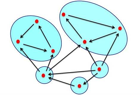
Figure 1: The condensation of a graph.

Consider an infinite sequence $(g_{k})_{k>0}$ of digraphs over a fixed set of labelled vertices. A temporal random walk is defined by picking a starting vertex, moving to a random neighbor in $g_{1}$, then a random neighbor in $g_{2}$, and so on, forever [10, 11, 20, 25, 33]. Note that a temporal walk might not match a path in any of the graphs. How would one classify the states of this “dynamic” Markov chain? Repeating the condensation decomposition at each step makes little sense, as it carries no information about the temporal walks. Instead, we want to monitor when and where temporal walks are extended. The cumulant graph compiles all such extensions and, when the process stalls at time $t^{\prime}$, reboots it by restarting from scratch at $t=t^{\prime}$. We define a grammar with which we parse the sequence $(g_{k})_{k>0}$ accordingly. The method, explained in detail in the next section, is very general and likely to be useful elsewhere.

Markov influence systems.

All finite Markov chains oscillate periodically or mix to a stationary distribution. One key fact about their dynamics is that the timescales never exceed a single exponential in the number of states. Allowing the transition probabilities to fluctuate over time at random does not change that basic fact [3, 13, 14]. Markov influence systems are quite different in that regard. Postponing formal definitions, let us think of an MIS for now as a dynamical system defined by iterating the map $f\!:\mathbf{x}^{\top}\mapsto\mathbf{x}^{\top}S(\mathbf{x})$, where $\mathbf{x}$ is a probability distribution represented as a column vector in $\mathbb{R}^{n}$ and $S(\mathbf{x})$ is a stochastic matrix that is piecewise-constant as a function of $\mathbf{x}$. We assume that the discontinuities are flats (ie, affine subspaces). The assumption is not nearly as restrictive as it appears, as we explain with a simple example.

Consider a random variable $\xi$ over the distribution $\mathbf{x}$ and fix two $n$-by-$n$ stochastic matrices $A$ and $B$. Define $S(\mathbf{x})=A$ (resp. $B$) if $\text{\rm var}_{\mathbf{x}}\,\xi>1$ (resp. else); in other words, the random walk picks one of two stochastic matrices at each step depending on the variance of $\xi$ with respect to the current state distribution $\mathbf{x}$. Note that, in violation of our assumption, the discontinuity is quadratic in $\mathbf{x}$. This is not an issue because we can always linearize the variance: we begin with the identity $\text{\rm var}_{\mathbf{x}}\,\xi=\frac{1}{2}\sum_{i,j}\,(\xi_{i}-\xi_{j})^{2}x_{i}x_{j}$ and the fact that $\mathbf{y}\!:=(x_{i}x_{j})_{i,j}$ is a probability distribution. We form the Kronecker square $T(\mathbf{y})=S(\mathbf{x})\otimes S(\mathbf{x})$ and lift the system into the $(n^{2}-1)$-dimensional unit simplex to get a brand-new MIS defined by the map $\mathbf{y}^{\top}\mapsto\mathbf{y}^{\top}T(\mathbf{y})$. We now have linear discontinuities. This same type of tensor lift can be used to linearize any algebraic constraints; this requires making the polynomials over $x_{i}$ homogeneous, which we can do by using the identity $\sum_{i}x_{i}=1$. Using ideas from [8], one can go even further than that and base the stepwise edge selection on the outcome of any first-order logical formula we may fancy (with the $x_{i}$’s acting as free variables). The key fact behind this result is that the first-order theory of the reals is decidable by quantifier elimination. This allows us to pick the next stochastic matrix at each time step on the basis of the truth value of a Boolean logic formula with arbitrarily many quantifiers (see [8] for details). This discussion is meant to highlight the fact that assuming linear discontinuities is not truly restrictive.

We prove in this article that an irreducible Markov influence system is almost always asymptotically periodic. (An MIS is irreducible if $S(\mathbf{x})$ forms an irreducible chain for each $\mathbf{x}$.) We extend this result to larger families of Markov influence systems. We also give an example of “hyper-torpid” mixing: an MIS that converges to a stationary distribution in time equal to a tower-of-twos in the size of the chain. This bound also applies to the period of certain periodic MIS. The emergence of timescales far beyond the reach of standard Markov chains is a distinctive feature of Markov influence systems.

Unlike in a standard random walk, the noncontractive eigenspace of an MIS may vary over time. It is this spectral incoherence that renormalization attempts to “tame.” To see why this has a strong graph-theoretic flavor, observe that at each time step the support of the stationary distribution can be read off the topology of the current graph: for example, the number of sinks in the condensation is equal to the dimension of the principal eigenspace plus one. Renormalization can thus be seen as an attempt to restore coherence to an ever-changing spectral landscape via a dynamic hierarchy of graphs, subgraphs, and homomorphs.

The bifurcation analysis at the heart of the analysis depends on a notion of “general position” aimed at bounding the growth rate of the induced symbolic dynamics [5, 22, 34]. The root of the problem is a clash between order and randomness similar to the conflict between entropy and energy encountered in the Ising model. The tension between these two “forces” is mediated by the critical values of a perturbation parameter, which are shown to form a Cantor set of Hausdorff dimension strictly less than 1. Final remark: There is a growing body of literature on dynamic graphs [2, 4, 7, 17, 20, 23, 25, 26, 29, 30] and their random walks [3, 10, 11, 12, 16, 13, 14, 21, 27, 28, 31, 33]. What distinguishes this work from its predecessors is that the changes in topology are induced endogenously by the system itself (via a feedback loop).

2 How to Parse a Graph Sequence

Throughout this work, a digraph refers to a directed graph with vertices in $[n]\!:=\{1,\ldots,n\}$ and a self-loop at each vertex. Graphs and digraphs (words we use interchangeably) have no multiple edges. We denote digraphs by lower-case letters ($g,h$, etc) and use boldface symbols for sequences. A digraph sequence $\mathbf{g}=(g_{k})_{k>0}$ is an ordered, finite or infinite, list of digraphs over the vertex set $[n]$. The digraph $g_{i}\times g_{j}$ consists of all the edges $(x,y)$ such that there exist an edge $(x,z)$ in $g_{i}$ and another one $(z,y)$ in $g_{j}$ for at least one vertex $z$. The operation $\times$ is associative but not commutative; it corresponds roughly to matrix multiplication. We define the cumulant $\prod_{\leq k}\mathbf{g}=g_{1}\times\cdots\times g_{k}$ and write $\prod\mathbf{g}=g_{1}\times g_{2}\times\cdots$ for finite $\mathbf{g}$. The cumulant indicates all the pairs of vertices that can be joined by a temporal walk of a given length. The mixing time of a random walk on a (fixed) graph depends on the speed at which information propagates and, in particular, how quickly the cumulant becomes transitive. In the time-varying case, mixing is a more complicated proposition, but the emergence of transitive cumulants is still what guides the parsing process.

An edge $(x,y)$ of a digraph $g$ is leading if there is $u$ such that $(u,x)$ is an edge of $g$ but $(u,y)$ is not. The non-leading edges form a subgraph of $g$, which is denoted by $\text{\em{tf}}\,(g)$ and called the transitive front of $g$. For example, $\text{\em{tf}}\,(x\rightarrow y\rightarrow z)$ is the graph over $x,y,z$ with the single edge $x\rightarrow y$ (and the three self-loops); on the other hand, the transitive front of a directed cycle over three or more vertices has no edges besides the self-loops. We denote by $\text{\em{cl}}(g)$ the transitive closure of $g$: it is the graph that includes an edge $(x,y)$ for any two vertices $x,y$ with a path from $x$ to $y$. Note that $\text{\em{tf}}\,(g)\preceq g\preceq\text{\em{cl}}(g)$.

• An equivalent definition of the transitive front is that the edges of $\text{\em{tf}}\,(g)$ are precisely the pairs $(i,j)$ such that $C_{i}\subseteq C_{j}$, where $C_{k}$ denotes the set of vertices $l$ such that $(l,k)$ is an edge of $g$. Because each vertex has a self-loop, the inclusion $C_{i}\subseteq C_{j}$ implies that $(i,j)$ is an edge of $g$. If $g$ is transitive, then $\text{\em{tf}}\,(g)=g$. The set-inclusion definition of the transitive front shows that it is indeed transitive: ie, if $(x,y)$ and $(y,z)$ are edges, then so is $(x,z)$. Given two graphs $g,h$ over the same vertex set, we write $g\preceq h$ if all the edges of $g$ are in $h$ (with strict inclusion denoted by the symbol $\prec$). Because of the self-loops, $g,h\preceq g\times h$.

• A third characterization of $\text{\em{tf}}\,(g)$ is as the unique densest graph $h$ over $[n]$ such that $g\times h=g$: we call this the maximally-dense property of the transitive front, and it is the motivation behind our use of the concept. Indeed, the failure of subsequent graphs to grow the cumulant implies a structural constraint on them. This is the sort of structure that parsing attempts to tease out.

The parser.

The parse tree of a (finite or infinite) graph sequence $\mathbf{g}=(g_{k})_{k>0}$ is a rooted tree whose leaves are associated with $g_{1},g_{2},\ldots$ from left to right. The purpose of the parse tree is to monitor the formation of new temporal walks as time progresses. This is based on the observation that, because of the self-loops, the cumulant $\prod_{\leq k}\mathbf{g}$ is monotonically nondecreasing with $k$ (with all references to graph ordering being relative to $\preceq$). If the increase were strict at each step then the parse tree would look like a fishbone. But, of course, the increase cannot go on forever. To continue to extract structure even when the cumulant is “stuck” is what parsing is all about. The underlying grammar consists of three productions: (1a) and (1b) renormalize the graph sequence along the time axis, while (2) creates the hierarchical clustering of the graphs in the sequence $\mathbf{g}$.

1. Temporal renormalization     We express the sequence $\mathbf{g}$ in terms of minimal subsequences with cumulants equal to $\prod\mathbf{g}$. There is a unique decomposition

   $$\mathbf{g}=\mathbf{g}_{1},g_{m_{1}},\ldots,\mathbf{g}_{k},g_{m_{k}},\mathbf{g}_{k+1}$$

   such that

   • $\mathbf{g}_{1}=g_{1},\ldots,g_{m_{1}-1}$; $\mathbf{g}_{i}=g_{m_{i-1}+1},\ldots,g_{m_{i}-1}$ ($1<i\leq k$); and $\mathbf{g}_{k+1}=g_{m_{k}+1},\ldots\,$.

   • $\bigl{(}\prod\mathbf{g}_{i}\bigr{)}\times g_{m_{i}}=\prod\mathbf{g}$, for any $i\leq k$; and $\prod\mathbf{g}_{i}\prec\prod\mathbf{g}$, for any $i\leq k+1$.

   The two productions below create the temporal parse tree.

   • Transitivization. Assume that $\prod\mathbf{g}$ is not transitive. We define $h=\text{\em{tf}}\,(\prod\mathbf{g})$ and note that $h\prec\prod\mathbf{g}$. It follows from the maximally-dense property of the transitive front that $k=1$. Indeed, $k>1$ implies that $\prod\mathbf{g}=\bigl{(}\prod\mathbf{g}_{2}\bigr{)}\times g_{m_{2}}\preceq\text{\em{tf}}\,\bigl{\{}\bigl{(}\prod\mathbf{g}_{1}\bigr{)}\times g_{m_{1}}\bigr{\}}=\text{\em{tf}}\,(\prod\mathbf{g})$, which contradicts the non-transitivity of $\prod\mathbf{g}$. We have the production

     $$\mathbf{g}\,\,\longrightarrow\,\,\bigl{(}\,\mathbf{g}_{1}\bigr{)}\,g_{m_{1}}\,\bigl{(}\,(\mathbf{g}_{2})\bigtriangleup h\,\bigr{)},$$ (1a)

     In the parse tree, the node for $\mathbf{g}$ has three children: the first one serves as the root of the temporal parse subtree for $\mathbf{g}_{1}$; the second one is the leaf associated with the graph $g_{m_{1}}$; the third one is a special node annotated with the label $h$, which serves as the parent $v$ of the node $w$ rooting the parse subtree for $\mathbf{g}_{2}$. The node $w$ is labeled (implicitly) by the transitive graph $\text{\em{cl}}(\prod\mathbf{g}_{2})$, which serves as a coarse-grained approximation of $\prod\mathbf{g}_{2}$. The purpose of annotating a special node with the label $h$ is to provide an intermediate approximation of $\prod\mathbf{g}_{2}$ that is strictly finer than the “obvious” $\text{\em{cl}}(\prod\mathbf{g})$. These coarse-grained approximations are called sketches.

   • Cumulant completion. Assume that $\prod\mathbf{g}$ is transitive. We have the production

     $$\mathbf{g}\,\,\longrightarrow\,\,\bigl{(}\,\mathbf{g}_{1}\bigr{)}\,g_{m_{1}}\,\bigl{(}\,\mathbf{g}_{2}\bigr{)}\,g_{m_{2}}\,\cdots\bigl{(}\,\mathbf{g}_{k}\bigr{)}\,g_{m_{k}}\,\bigl{(}\,\mathbf{g}_{k+1}\bigr{)}.$$ (1b)

     Note that the index $k$ may be infinite and any of the subsequences $\mathbf{g}_{i}$ might be empty (for example, $\mathbf{g}_{k+1}$ if $k=\infty$).

2. Topological renormalization     Network renormalization exploits the fact that the information flowing across the system might get stuck in portions of the graph for some period of time: when this happens, we cluster the graphs using topological renormalization. As we just discussed, each node $v$ of the temporal parse tree that is not annotated by (1a) is labeled by the sketch $\text{\em{cl}}(\prod\mathbf{g})$, where $\mathbf{g}$ is the graph sequence formed by the leaves of the subtree rooted at $v$. In this way, every path from the root of the temporal parse tree comes with a nested sequence of sketches $h_{1}\succeq\cdots\succeq h_{l}$. Pick two consecutive ones, $h_{i},h_{i+1}$: these are two transitive graphs whose strongly connected components, therefore, are cliques. Let $V_{1},\ldots,V_{a}$ and $W_{1},\ldots,W_{b}$ be the vertex sets of the cliques corresponding to $h_{i}$ and $h_{i+1}$, respectively. Since $h_{i+1}$ is a subgraph of $h_{i}$, it follows that each $V_{i}$ is a disjoint union of the form $W_{i_{1}}\cup\cdots\cup W_{i_{s_{i}}}$.

   • Decoupling. We decorate the temporal parse tree with an additional tree connecting the sketches present along each one of its paths. These topological parse trees are formed by all the productions of the type:

     $$V_{i}\,\,\longrightarrow\,\,W_{i_{1}}\cdots W_{i_{s_{i}}}.$$ (1)

     A sketch at a node $v$ of the temporal tree can be viewed as an acyclic digraph over cliques: its purpose is to place limits on the movement of the probability mass in any temporal random walk corresponding to the leaves of the subtree rooted at $v$. In particular, it indicates how decoupling might arise in the system.

The maximum depth of the temporal parse tree is $O(n^{2})$ because each child’s cumulant loses at least one edge from its parent’s (or grandparent’s) cumulant. To see why the quadratic bound is tight, consider a bipartite graph $V=L\cup R$, where $|L|=|R|$ and each pair from $L\times R$ is added one at a time as a bipartite graph with a single nonloop edge; the leftmost path of the parse tree is of quadratic length.

Left-to-right parsing.

The temporal tree can be built on-line by scanning the graph sequence $\mathbf{g}$ with no need to back up. Let $\mathbf{g^{\prime}}$ denote the sequence formed by appending the graph $g$ to the end of the finite graph sequence $\mathbf{g}$. If $\mathbf{g}$ is empty, then the tree $\mathcal{T}(\mathbf{g^{\prime}})$ consists of a root with one child labeled $g$. If $\mathbf{g}$ is not empty and $\prod\mathbf{g}\prec\prod\mathbf{g^{\prime}}$, the root of $\mathcal{T}(\mathbf{g^{\prime}})$ has one child formed by the root of $\mathcal{T}(\mathbf{g})$ as well as a child labeled $g$. Assume now that $\mathbf{g}$ is not empty and that $\prod\mathbf{g}=\prod\mathbf{g^{\prime}}$. Let $v$ be the lowest internal node on the rightmost path of $\mathcal{T}(\mathbf{g})$ such that $c_{v}\times g=c_{v}$, where $c_{u}$ denotes the product of the graphs associated with the leaves of the subtree rooted at node $u$ of $\mathcal{T}(\mathbf{g})$. Let $w$ be the rightmost child of $v$; note that $v$ and $w$ always exist. We explain how to form $\mathcal{T}(\mathbf{g^{\prime}})$ by editing $\mathcal{T}(\mathbf{g})$.

1. $c_{v}$ is transitive and $w$ is a leaf: We add a leaf labeled $g$ as the new rightmost child $z$ of $v$ if $g=c_{v}$; otherwise, we do the same but, instead of attaching $g$ directly to $v$, we make it the unique child of $z$.

2. $c_{v}$ is transitive and $w$ is not a leaf: We add a leaf labeled $g$ as the new rightmost child of $v$ if $c_{w}\times g=c_{v}$; otherwise, we add a new rightmost child $z$ to $v$ and we give $z$ two children: its left child is $w$ and its subtree below; its right child is a leaf labeled $g$.

3. $c_{v}$ is not transitive and $w$ is a leaf: We attach a new rightmost child $z$ to $v$, and we make it a special node annotated with the label $\text{\em{tf}}\,(c_{v})$. We give $z$ a single child $z^{\prime}$, which is itself the parent of a new leaf labeled $g$.

4. $c_{v}$ is not transitive and $w$ is not a leaf: We note that $c_{w}\times g\preceq\text{\em{tf}}\,(c_{v})\prec c_{v}$. We attach a new rightmost child $z$ to $v$, and we make it a special node annotated with the label $\text{\em{tf}}\,(c_{v})$. We give $z$ a single child $z^{\prime}$, to which we attach two children: one of them is $w$ (and its subtree) and the other one is the leaf labeled $g$.

Undirected graphs.

A graph is called undirected if any edge $(x,y)$ with $x\neq y$ comes with its companion $(y,x)$. Consider a sequence of undirected graphs over $[n]$. We begin with the observation that the cumulant of a subsequence might itself be directed; for example, the product $g_{1}\times g_{2}=(x\leftrightarrow y\ \ \ \ z)\times(x\ \ \ \ y\leftrightarrow z)$ has a directed edge from $x$ to $z$ but not from $z$ to $x$. We can use undirectedness to strengthen the definition of the transitive front. Recall that $\text{\em{tf}}\,(g)$ is the unique densest graph $h$ such that $g\times h=g$. Its purpose is the following: if $g$ is the current cumulant, the transitive front of $g$ is intended to include any edge that might appear in subsequent graphs in the sequence without extending any path in $g$. Since, in the present case, the only edges considered for extension will be undirected, we might as well require that $h$ itself (unlike $g$) should be undirected. In this way, we redefine the transitive front, now denoted by $\text{\em{utf}}\,(g)$, as the unique densest undirected graph $h$ such that $g\times h=g$. Its edge set includes all the pairs $(i,j)$ such that $C_{i}=C_{j}$. Because of self-loops, the condition implies that $(i,j)$ is an undirected edge of $g$. This forms an equivalence relation among the vertices, so that $\text{\em{utf}}\,(g)$ actually consists of disconnected, undirected cliques. To see the difference with the directed case, we take our previous example and note that $\text{\em{tf}}\,(g_{1}\times g_{2})$ has the edges $(x,y),(x,z),(y,z),(z,y)$ in addition to the self-loops, whereas $\text{\em{utf}}\,(g_{1}\times g_{2})$ has the single undirected edge $(y,z)$ plus self-loops.

The depth of the parse tree can still be as high as quadratic in $n$. To see why, consider the following recursive construction. Given a clique $C_{k}$ over $k$ vertices $x_{1},\ldots,x_{k}$ at time $t$, attach to it, at time $t+1$, the undirected edge $(x_{1},y)$. The cumulant gains the undirected edge $(x_{1},y)$ and the directed edges $(x_{i},y)$ for $i=2,\ldots,k$. At time $t+2,\ldots,t+k$, visit each one of the $k-1$ undirected edges $(x_{1},x_{i})$ for $i>1$, using single-edge undirected graphs. Each such step will see the addition of a new directed edge $(y,x_{i})$ to the cumulant, until it becomes the undirected clique $C_{k+1}$. The quadratic lower bound on the tree depth follows immediately.

Backward parsing.

The sequence of graphs leads to products where each new graph is multiplied to the right, as would happen in a time-varying Markov chain. Algebraically, the matrices are multiplied from left to right. In diffusive systems (eg, multiagent agreement systems, Hegselmann-Krause models, Deffuant systems), however, matrices are multiplied from right to left. Although the dynamics can be quite different, the same parsing algorithm can be used. Given a sequence $\mathbf{g}=(g_{k})_{k>0}$, its backward parsing is formed by applying the parser to the sequence $\overleftarrow{\,\mathbf{g}}=(h_{k})_{k>0}$, where $h_{k}$ is derived from $g_{k}$ by reversing the direction of every edge, ie, $(x,y)$ becomes $(y,x)$. Once the parse tree for $\overleftarrow{\,\mathbf{g}}$ has been built, we simply restore each edge to its proper direction to produce the backward parse tree of $\mathbf{g}$.

3 The Markov Influence Model

Let $\mathbb{S}^{n-1}$ (or $\mathbb{S}$ when the dimension is understood) be the standard simplex $\bigl{\{}\,\mathbf{x}\in\mathbb{R}^{n}\,|\,\,\mathbf{x}\geq\mathbf{0}\,,\,\|\mathbf{x}\|_{1}=1\,\bigr{\}}$ and let $\mathcal{S}$ denote set of all $n$-by-$n$ rational stochastic matrices. A Markov influence system (MIS ) is a discrete-time dynamical system with phase space $\mathbb{S}$, which is defined by the map $f\!:\mathbf{x}^{\top}\mapsto f(\mathbf{x})\!:=\mathbf{x}^{\top}S\!(\mathbf{x})$, where $\mathbf{x}\in\mathbb{S}$ and $S$ is a function $\mathbb{S}\mapsto\mathcal{S}$ that is constant over the pieces of a finite polyhedral partition $\mathcal{P}\!=\!\{P_{k}\}$ of $\mathbb{S}$; we define $f$ as the identity on the discontinuities of the partition (fig.2).

(i)  We define the digraph $g(\mathbf{x})$ (and its corresponding Markov chain) formed by the positive entries of $S\!(\mathbf{x})$. To avoid inessential technicalities, we assume that the diagonal of each $S\!(\mathbf{x})$ is strictly positive (ie, $g(\mathbf{x})$ has self-loops). In this way, any orbit of an MIS corresponds to a lazy, time-varying random walk with transitions defined endogenously. We recall some basic terminology. The orbit of $\mathbf{x}\in\mathbb{S}$ is the infinite sequence $(f^{t}(\mathbf{x}))_{t\geq 0}$ and its itinerary is the corresponding sequence of cells $P_{k}$ visited in the process. The orbit is periodic if $f^{t}(\mathbf{x})=f^{s}(\mathbf{x})$ for any $s=t$ modulo a fixed integer. It is asymptotically periodic if it gets arbitrarily close to a periodic orbit over time.

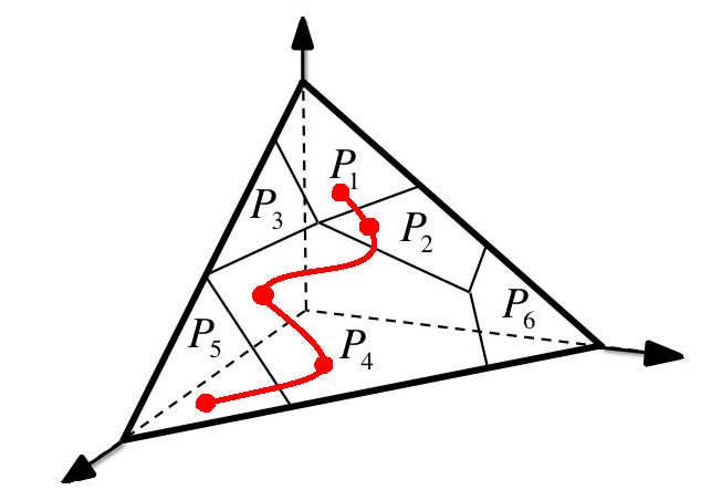
Figure 2: A Markov influence system: each region $P_{k}$ is associated with a single stochastic matrix. The first five steps of an orbit are shown to visit regions $P_{1},P_{2},P_{4},P_{4},P_{5}$ in this order.

(ii)  The discontinuities in $\mathcal{P}$ are formed by hyperplanes in $\mathbb{R}^{n}$ of the form $\mathbf{a}_{i}^{\top}\mathbf{x}=1+\delta$, where $\delta$ is confined to an interval $\Omega:=[-\omega,\omega]$. Assuming general position, we can pick a small positive $\omega<1/2$ so that $\mathcal{P}$ remains (topologically) the same over $\Omega$. Thus, the MIS remains well-defined for all $\delta\in\Omega$. As we show in Section 5, the parameter $\delta$ is necessary to keep chaos at bay.

(iii)  The coefficient of ergodicity $\tau(M)$ of a matrix $M$ is defined as half the maximum $\ell_{1}$-distance between any two of its rows [32]. It is submultiplicative for stochastic matrices, a direct consequence of the identity $\tau(M)=\max\,\Bigl{\{}\,\|\mathbf{x}^{\top}M\|_{1}:\mathbf{x}^{\top}\mathbf{1}=0\hskip 5.69046pt\text{and}\hskip 5.69046pt\|\mathbf{x}\|_{1}=1\,\Bigr{\}}$.

(iv)  Given $\Delta\subseteq\Omega$, let $L_{\Delta}^{t}$ denote the set of $t$-long prefixes of any itinerary for any starting position $\mathbf{x}\in\mathbb{S}$ and any $\delta\in\Delta$. We define the ergodic renormalizer $\eta_{\Delta}$ as the smallest integer such that, for any $t\geq\eta_{\Delta}$ and any matrix sequence $S_{\!1},\ldots,S_{\!t}$ associated with an element of $L_{\Delta}^{t}$, the product $S_{\!1}\cdots S_{\!t}$ is primitive (ie, some high enough power is a positive matrix) and its coefficient of ergodicity is less than $1/2$. We assume in this section that $\eta\!:=\eta_{\Omega}<\infty$ and discuss in Section 4 how to relax this assumption via renormalization. Let $D$ be the union of the hyperplanes from $\mathcal{P}$ in $\mathbb{R}^{n}$ (where $\delta$ is understood). We define $Z_{t}=\bigcup_{0\leq k\leq t}f^{-k}(D)$ and $Z=\bigcup_{t\geq 0}Z_{t}$. Note that $Z\subseteq\mathbb{S}$ since the latter is the domain of $f$. Remarkably, for almost all $\delta\in\Omega$, $Z_{t}$ becomes strictly equal to $Z$ in a finite number of steps.

Lemma 3.1

$\!\!\!.\,\,$ There is a constant $c>0$ such that, for any $\varepsilon>0$, there exists an integer $\nu\leq 2^{\eta^{c}}\log(1/\varepsilon)$ and a finite union $K$ of intervals of total length less than $\varepsilon$ such that $Z_{\nu}=Z_{\nu-1}$, for any $\delta\in\Omega\setminus K$.

Note that $Z_{\nu}=Z_{\nu-1}$ implies that $Z=Z_{\nu}$. Indeed, suppose that $Z_{t+1}\supset Z_{t}$ for $t\geq\nu$; then, $f^{t+1}(\mathbf{y})\in D$ but $f^{t}(\mathbf{y})\not\in D$ for some $\mathbf{y}\in\mathbb{S}$; in other words, $f^{\nu}(\mathbf{x})\in D$ but $f^{\nu-1}(\mathbf{x})\not\in D$ for $\mathbf{x}=f^{t-\nu+1}(\mathbf{y})$, which contradicts the equality $Z_{\nu}=Z_{\nu-1}$.

Corollary 3.2

$\!\!\!.\,\,$ For $\delta$ almost everywhere in $\Omega$, every orbit is asymptotically periodic.

Proof. The equality $Z=Z_{\nu}$ implies the eventual periodicity of the symbolic dynamics. The period cannot exceed the number of connected components in the complement of $Z$. Once an itinerary becomes periodic at time $t_{o}$ with period $\sigma$, the map $f^{t}$ can be expressed locally by matrix powers. Indeed, divide $t-t_{o}$ by $\sigma$ and let $q$ be the quotient and $r$ the remainder; then, locally, $f^{t}=g^{q}\circ f^{t_{o}+r}$, where $g$ is specified by a stochastic matrix with a positive diagonal, which implies convergence to a periodic point at an exponential rate. Finally, apply Lemma 3.1 repeatedly, with $\varepsilon=2^{-l}$ for $l=1,2,\ldots$ and denote by $K_{l}$ be the corresponding union of “forbidden” intervals. Define $K^{l}=\bigcup_{j\geq l}K_{j}$ and $K^{\infty}=\bigcap_{l>0}K^{l}$; then Leb$(K^{l})\leq 2^{1-l}$ and hence Leb$(K^{\infty})=0$. The lemma follows from the fact that any $\delta\in\Omega$ outside of $K^{\infty}$ lies outside of $K^{l}$ for some $l>0$. $\Box$

The corollary states that the set of “nonperiodic” values of $\delta$ has measure zero in parameter space. Our result is actually stronger than that. We prove that the nonperiodic set can be covered by a Cantor set of Hausdorff dimension strictly less than 1. The remainder of this section is devoted to a proof of Lemma 3.1.

3.1 Shift spaces and growth rates

The growth exponent of a language is defined as $\lim_{n\rightarrow\infty}\frac{1}{n}\max_{k\leq n}\log N(k)$, where $N(k)$ is the number of words of length $k$; for example, the growth exponent of $\{0,1\}^{*}$ is 1 (all logarithms taken to the base 2). The language consisting of all the itineraries of a Markov influence system forms a shift space and its growth exponent is the topological entropy of its symbolic dynamics [34]—not to be confused with the topological entropy of the MIS itself. It can be strictly positive, which is a sign of chaos. We show that, for a typical system, it is zero, the key fact underlying periodicity. Let $M_{1},\ldots,M_{T}$ be $n$-by-$n$ matrices from a finite set $\mathcal{M}$ of primitive stochastic rational matrices with positive diagonals, and assume that $\tau(M)<1/2$ for $M\in\mathcal{M}$; hence $\tau(M_{1}\cdots M_{k})<2^{-k}$. Because each product $M_{1}\cdots M_{k}$ is a primitive matrix, it can be expressed as $\mathbf{1}\bm{\pi}_{k}^{\top}+Q_{k}$ (by Perron-Frobenius), where $\bm{\pi}_{k}$ is its (unique) stationary distribution. If $\bm{\pi}$ is a stationary distribution for a stochastic matrix $S$, then its $j$-th row $\bm{s}_{j}$ satisfies $\bm{s}_{j}-\bm{\pi}^{\top}=\bm{s}_{j}-\bm{\pi}^{\top}S=\sum_{i}\bm{\pi}_{i}(\bm{s}_{j}-\bm{s}_{i})$; hence, by the triangular inequality, $\|\bm{s}_{j}-\bm{\pi}^{\top}\|_{1}\leq\sum_{i}\pi_{i}\|\bm{s}_{j}-\bm{s}_{i}\|_{1}\leq 2\tau(S)$. This implies that

$$\begin{cases}\hskip 5.69046ptM_{1}\cdots M_{k}=\mathbf{1}\bm{\pi}_{k}^{\top}+Q_{k}\\ \hskip 5.69046pt\|Q_{k}\|_{\infty}\leq 2\tau(M_{1}\cdots M_{k})<2^{1-k}.\end{cases}$$ (2)

Property $\mathbf{U}$.

Fix a vector $\mathbf{a}\in\mathbb{Q}^{n}$, and denote by $M^{\,(\theta)}$ the $n$-by-$m$ matrix with the $m$ column vectors $M_{1}\cdots M_{k_{i}}\,\mathbf{a}$, where $\theta=(k_{1},\ldots,k_{m})$ is an increasing sequence of integers in $[T]$. We say that property $\mathbf{U}$ holds if there exists a rational vector $\mathbf{u}=\mathbf{u}(\theta)$ such that $\mathbf{1}^{\top}\mathbf{u}=1$ and $\mathbf{x}^{\top}M^{\,(\theta)}\mathbf{u}$ does not depend on the variable $\mathbf{x}\in\mathbb{S}$. Property $\mathbf{U}$ is a quantifier elimination device for expressing a notion of “general position” for an MIS. To see why, consider a simple statement such as “the three points $\bigl{(}x,x^{2}\bigr{)}$, $\bigl{(}x+1,(x+1)^{2}\bigr{)}$, and $\bigl{(}x+2,(x+2)^{2}\bigr{)}$ cannot be collinear for any value of $x$.” This can be expressed by saying that a certain determinant polynomial in $x$ is constant. Likewise, the vector $\mathbf{u}$ manufactures a quantity, $\mathbf{x}^{\top}M^{\,(\theta)}\mathbf{u}$, that “eliminates” the variable $\mathbf{x}$. Some condition on $\mathbf{u}$ is needed since otherwise we could pick $\mathbf{u}=\mathbf{0}$. Note that property $\mathbf{U}$ would be obvious if all the matrices $Q_{k}$ in (2) were null: indeed, we would have $\mathbf{x}^{\top}M^{\,(\theta)}=\mathbf{x}^{\top}\mathbf{1}(b_{1},\ldots,b_{m})=(b_{1},\ldots,b_{m})$, where $b_{i}=\bm{\pi}_{k_{i}}^{\top}\,\mathbf{a}$. This suggests that property $\mathbf{U}$ rests on the decaying properties of $Q_{k}$.

To see the relevance of general position to the dynamics of an MIS, consider the iterates of a small ball through the map $f$. To avoid chaos, it is intuitively obvious that these iterated images should not fall across discontinuities too often. Fix such a discontinuity: if we think of the ball as being so small it looks like a point, then the case we are trying to avoid consists of many points (the ball’s iterates) lying on (or near) a given hyperplane. This is similar to the definition of general position, which requires that a set of point should not lie on the same hyperplane.

Lemma 3.3

$\!\!\!.\,\,$ There exists a constant $b>0$ (linear in $n$) such that, given any integer $T>0$ and any increasing sequence $\theta$ in $[T]$ of length at least $T^{1-\alpha}/\alpha$, property $\mathbf{U}$ holds, where $\alpha\!:=\mu^{-b}$ and $\mu$ is the maximum number of bits needed to encode any entry of $M_{k}$ for any $k\in[T]$.

Proof. By choosing $b$ large enough, we can ensure that $T$ is as big as we want. The proof is a mixture of algebraic and combinatorial arguments. We begin with a Ramsey-like statement about stochastic matrices.

Fact 3.4

$\!\!\!.\,\,$ There is a constant $d>0$ such that, if the sequence $\theta$ contains $j_{0},\ldots,j_{n}$ with $j_{i}\geq d\mu j_{i-1}$ for each $i\in[n]$, then property $\mathbf{U}$ holds.

Proof. By (2), $\|Q_{k}\mathbf{a}\|_{\infty}<c_{0}2^{-k}$ for constant $c_{0}>0$. Note that $Q_{k}$ has rational entries over $O(\mu k)$ bits: the bound follows from the fact that the stationary distribution $\bm{\pi}_{k}$ has rational coordinates over $O(\mu k)$ bits; as noted earlier, the constant factors may depend on $n$. We write $M^{\,(\theta)}=\mathbf{1}\mathbf{a}^{\top}\Pi^{\,(\theta)}+Q^{\,(\theta)}$, where $\Pi^{\,(\theta)}$ and $Q^{\,(\theta)}$ are the $n$-by-$m$ matrices formed by the $m$ column vectors $\bm{\pi}_{k_{i}}$ and $Q_{k_{i}}\mathbf{a}$, respectively, for $i\in[m]$; recall that $\theta=(k_{1},\ldots,k_{m})$. The key fact is that the dependency on $\mathbf{x}\in\mathbb{S}$ is confined to the term $Q^{\,(\theta)}$: indeed,

$$\mathbf{x}^{\top}M^{\,(\theta)}\mathbf{u}=\mathbf{a}^{\top}\Pi^{\,(\theta)}\mathbf{u}+\mathbf{x}^{\top}Q^{\,(\theta)}\mathbf{u}.$$ (3)

This shows that, in order to satisfy property $\mathbf{U}$, it is enough to ensure that $Q^{\,(\theta)}\mathbf{u}=0$ has a solution such that $\mathbf{1}^{\top}\mathbf{u}=1$. Let $\sigma=(j_{0},\ldots,j_{n-1})$. If $Q^{\,(\sigma)}$ is nonsingular then, because each one of its entries is a rational over $O(\mu j_{n-1})$ bits, we have $|\det Q^{\,(\sigma)}|\geq c_{1}^{\mu j_{n-1}}$, for constant $c_{1}>0$. Let $R$ be the $(n+1)$-by-$(n+1)$ matrix derived from $Q^{\,(\sigma)}$ by adding the column $Q_{j_{n}}\mathbf{a}$ to its right and then adding a row of ones at the bottom. If $R$ is nonsingular, then $R\,\mathbf{u}=(0,\ldots,0,1)^{\top}$ has a (unique) solution in $\mathbf{u}$ and property $\mathbf{U}$ holds (after padding $\mathbf{u}$ with zeroes). Otherwise, we expand the determinant of $R$ along the last column. Suppose that $\det Q^{\,(\sigma)}\neq 0$. By Hadamard’s inequality, all the cofactors are at most a constant $c_{2}>0$ in absolute value; hence, for $d$ large enough,

$$0=|\det R\,|\geq|\det Q^{\,(\sigma)}\,|-nc_{2}\|Q_{j_{n}}\mathbf{a}\,\|_{\infty}\geq c_{1}^{\mu j_{n-1}}-nc_{2}c_{0}2^{-j_{n}}>0.$$

This contradiction implies that $Q^{\,(\sigma)}$ is singular, so (at least) one of its rows can be expressed as a linear combination of the others. We form the $n$-by-$n$ matrix $R^{\prime}$ by removing that row from $R$, together with the last column, and setting $u_{j_{n}}=0$ to rewrite $Q^{\,(\theta)}\mathbf{u}=0$ as $R^{\prime}\mathbf{u^{\prime}}=(0,\ldots,0,1)^{\top}$, where $\mathbf{u^{\prime}}$ is the restriction of $\mathbf{u^{\prime}}$ to the columns indexed by $R^{\prime}$. Having reduced the dimension of the system by one variable, we can proceed inductively in the same way; either we terminate with the discovery of a solution or the induction runs its course until $n=1$ and the corresponding 1-by-1 matrix is null, so that the solution 1 works. Note that $\mathbf{u}$ has rational coordinates over $O(\mu T)$ bits. $\Box$

Let $N(T)$ be the largest sequence $\theta$ in $[T]$ such that property $\mathbf{U}$ does not hold. Divide $[T]$ into bins $[(d\mu)^{k},(d\mu)^{k+1}-1]$ for $k\geq 0$. By Fact 3.4, the sequence $\theta$ can intersect at most $2n$ of them; thus, if $T>t_{0}$, for some large enough $t_{0}=(d\mu)^{O(n)}$, there is at least one empty interval in $T$ of length $T/(d\mu)^{2n+3}$. This gives us the recurrence $N(T)\leq T$ for $T\leq t_{0}$ and $N(T)\leq N(T_{1})+N(T_{2})$, where $T_{1}+T_{2}\leq\beta T$, for a positive constant $\beta=1-(d\mu)^{-2n-3}$. The recursion to the right of the empty interval, say, $N(T_{2})$, warrants a brief discussion. The issue is that the proof of Fact 3.4 relies crucially on the property that $Q_{k}$ has rational entries over $O(\mu k)$ bits—this is needed to lower-bound $|\!\det Q^{\,(\sigma)}|$ when it is not 0. But this is not true any more, because, after the recursion, the columns of the matrix $M^{\,(\theta)}$ are of the form $M_{1}\cdots M_{k}\,\mathbf{a}$, for $T_{1}+L<k\leq T$, where $L$ is the length of the empty interval and $T=T_{1}+L+T_{2}$. Left as such, the matrices use too many bits for the recursion to go through. To overcome this obstacle, we observe that the recursively transformed $M^{\,(\theta)}$ can be factored as $AB$, where $A=M_{1}\cdots M_{T_{1}+L}$ and $B$ consists of the column vectors $M_{T_{1}+L+1}\cdots M_{k}\,\mathbf{a}$. The key observation now is that, if $\mathbf{x}^{\top}B\,\mathbf{u}$ does not depend on $\mathbf{x}$, then neither does $\mathbf{x}^{\top}M^{\,(\theta)}\,\mathbf{u}$, since it can be written as $\mathbf{y}^{\top}B\,\mathbf{u}$ where $\mathbf{y}=A^{\top}\mathbf{x}\in\mathbb{S}$. In this way, we can enforce property $\mathbf{U}$ while having restored the proper encoding length for the entries of $M^{\,(\theta)}$.

Plugging in the ansatz $N(T)\leq t_{0}T^{\gamma}$, for some unknown positive $\gamma<1$, we find by Jensen’s inequality that, for all $T>0$, $N(T)\leq t_{0}(T_{1}^{\gamma}+T_{2}^{\gamma})\leq t_{0}2^{1-\gamma}\beta^{\gamma}T^{\gamma}$. For the ansatz to hold true, we need to ensure that $2^{1-\gamma}\beta^{\gamma}\leq 1$. Setting $\gamma=1/(1-\log\beta)<1$ completes the proof of Lemma 3.3. $\Box$

Define $\phi^{k}(\mathbf{x})=\mathbf{x}^{\top}M_{1}\cdots M_{k}$ for $\mathbf{x}\in\mathbb{R}^{n}$ and $k\leq T$; and let $h_{\delta}\!:\mathbf{a}^{\top}\mathbf{x}=1+\delta$ be some hyperplane in $\mathbb{R}^{n}$. We consider a set of canonical intervals of length $\rho$ (or less): $\mathcal{D}_{\rho}=\bigl{\{}\,[k\rho,(k+1)\rho]\cap\Omega\,|\,k\in\mathbb{Z}\,\bigr{\}}$, where $\rho>0$ (specified below), $\Omega=\omega\mathbb{I}$, $\mathbb{I}\!:=[-1,1]$, and $0<\omega<1/2$. Roughly, the “general position” lemma below says that, for most $\delta$, the $\phi^{k}$-images of any $\rho$-wide cube centered in the simplex $\mathbb{S}$ cannot come very near the hyperplane $h_{\delta}$ for most values of $k\leq T$. This may be counterintuitive. After all, if the stochastic matrices $M_{i}$ are the identity, the images stay put, so if the initial cube collides then all of the images will! The point is that $M_{i}$ is primitive so it cannot be the identity. The low coefficients of ergodicity will also play a key role. The crux of the lemma is that the exclusion set $U$ does not depend on the choice of $\mathbf{x}\in\mathbb{S}$. A point of notation: $\alpha$ refers to its use in Lemma 3.3.

Lemma 3.5

$\!\!\!.\,\,$ For any real $\rho>0$ and any integer $T>0$, there exists $U\subseteq\mathcal{D}_{\rho}$ of size $c_{T}=2^{O(\mu T)}$, where $c_{T}$ is independent of $\rho$, such that, for any $\Delta\in\mathcal{D}_{\rho}\!\setminus\!U$ and $\mathbf{x}\in\mathbb{S}$, there are at most $T^{1-\alpha}/\alpha$ integers $k\leq T$ such that $\phi^{k}(X)\cap h_{\Delta}\neq\emptyset$, where $X=\mathbf{x}+\rho\mathbb{I}^{n}$ and $h_{\Delta}\!:=\bigcup_{\delta\in\Delta}h_{\delta}$.

Proof. In what follows, $b_{0},b_{1},\ldots$ refer to suitably large positive constants (which, we shall recall, may depend on $n,\mathbf{a}$, etc). We assume the existence of more than $T^{1-\alpha}/\alpha$ integers $k\leq T$ such that $\phi^{k}(X)\cap h_{\Delta}\neq\emptyset$ for some $\Delta\in\mathcal{D}_{\rho}$ and draw the consequences: in particular, we infer certain linear constraints on $\delta$; by negating them, we define the forbidden set $U$ and ensure the conclusion of the lemma. Let $k_{1}<\cdots<k_{m}$ be the integers in question, where $m>T^{1-\alpha}/\alpha$. For each $i\in[m]$, there exists $\mathbf{x}(i)\in X$ and $\delta_{i}\in\Delta$ such that $|\,\mathbf{x}(i)^{\top}M_{1}\cdots M_{k_{i}}\mathbf{a}-1-\delta_{i}\,|\leq\rho$. Note that $|\delta_{i}-\delta|\leq\rho$ for some $\delta\in\Delta$ common to all $i\in[m]$. By the stochasticity of the matrices, it follows that $|\,\bigl{(}\mathbf{x}(i)-\mathbf{x}\bigr{)}^{\top}M_{1}\cdots M_{k_{i}}\mathbf{a}\,|\leq b_{0}\,\rho$; hence $|\,\mathbf{x}^{\top}M_{1}\cdots M_{k_{i}}\mathbf{a}-1-\delta\,|\leq(b_{0}+2)\rho$. By Lemma 3.3, there is a rational vector $\mathbf{u}$ such that $\mathbf{1}^{\top}\mathbf{u}=1$ and $\mathbf{x}^{\top}M^{\,(\theta)}\mathbf{u}=\psi(M^{\,(\theta)},\mathbf{a})$ does not depend on the variable $\mathbf{x}\in\mathbb{S}$; on the other hand, $|\,\mathbf{x}^{\top}M^{\,(\theta)}\mathbf{u}-(1+\delta)\,|\leq b_{1}\rho$. Two quick remarks: (i) the term $1+\delta$ is derived from $(1+\delta)\mathbf{1}^{\top}\mathbf{u}=1+\delta$; (ii) $b_{1}\leq(b_{0}+2)\|\mathbf{u}\|_{1}$, where $\mathbf{u}$ is a rational over $O(\mu T)$ bits. We invalidate the condition on $k_{1},\ldots,k_{m}$ by keeping $\delta$ outside the interval $\psi(M^{\,(\theta)},\mathbf{a})-1+b_{1}\rho\mathbb{I}$, which rules out at most $2(b_{1}+1)=2^{O(\mu T)}$ intervals from $\mathcal{D}_{\rho}$. Repeating this for all sequences $(k_{1},\ldots,k_{m})$ raises the number of forbidden intervals by a factor of at most $2^{T}$. $\Box$

Topological entropy.

We identify the family $\mathcal{M}$ with the set of all matrices of the form $S_{\!1}\cdots S_{\!k}$, for $\eta\leq k\leq 3\eta$ ($\eta=\eta_{\Omega}$), where the matrix sequence $S_{\!1},\ldots,S_{\!k}$ matches some element of $L_{\Omega}^{k}$. By definition of the ergodic renormalizer, any $M\in\mathcal{M}$ is primitive and $\tau(M)<1/2$; furthermore, both $\mu$ and $\log|\mathcal{M}\,|$ are in $O(\eta)$. Our next result shows that the topological entropy of the shift space of itineraries vanishes.

Lemma 3.6

$\!\!\!.\,\,$ For any real $\rho>0$ and any integer $T>0$, there exist $t_{\rho}=O(\eta|\log\rho\,|)$ and an exclusion set $V\subseteq\mathcal{D}_{\rho}$ of size $d_{T}=2^{O(T)}$ such that, for any $\Delta\in\mathcal{D}_{\rho}\!\setminus\!V$, any integer $t\geq t_{\rho}$, and any $\sigma\in L_{\Delta}^{t}$, $\log\,\bigl{|}\,\bigl{\{}\,\sigma^{\prime}\,|\,\sigma\cdot\sigma^{\prime}\in L_{\Delta}^{t+T}\,\bigr{\}}\,\bigr{|}\leq\eta^{b}T^{1-\eta^{-b}}$, for constant $b>0$.

Proof. In the lemma, $t_{\rho}$ (resp. $d_{T}$) is independent of $T$ (resp. $\rho$). The main point is that the exponent of $T$ is bounded away from 1. We define $V$ as the union of the sets $U$ formed by applying Lemma 3.5 to each one of the hyperplanes $h_{\delta}$ involved in $\mathcal{P}$ and every possible sequence of $T$ matrices in $\mathcal{M}$. This increases $c_{T}$ to $2^{O(\eta T)}$. Fix $\Delta\in\mathcal{D}_{\rho}\!\setminus\!V$ and consider the (lifted) phase space $\mathbb{S}\times\Delta$ for the dynamical system induced by the map $f_{\uparrow}\!:\bigl{(}\mathbf{x}^{\top},\delta)\mapsto(\,\mathbf{x}^{\top}S\!(\mathbf{x}),\delta\,\bigr{)}$. The system is piecewise-linear with respect to the polyhedral partition $\mathcal{P}_{\uparrow}$ of $\mathbb{R}^{n+1}$ formed by treating $\delta$ as a variable in $h_{\delta}$. Let $\Upsilon_{t}$ be a continuity piece for $f_{\uparrow}^{t}$, ie, a maximal region of $\mathbb{S}\times\Delta$ over which the $t$-th iterate of $f_{\uparrow}$ is linear. Reprising the argument leading to (2), any matrix sequence $S_{\!1},\ldots,S_{\!t}$ matching an element of $L_{\Delta}^{t}$ is such that $S_{\!1}\cdots S_{\!t}=\mathbf{1}\bm{\pi}^{\top}+Q$, where

$$\|Q\|_{\infty}<2^{2-t/\eta}.$$ (4)

Thus there exists $t_{\rho}=O(\eta|\log\rho\,|)$ such that, for any $t\geq t_{\rho}$, $f_{\uparrow}^{t}(\Upsilon_{t})\subseteq(\mathbf{x}+\rho\mathbb{I}^{n})\times\Delta$, for some $\mathbf{x}=\mathbf{x}(t,\Upsilon_{t})\in\mathbb{S}$. Consider a nested sequence $\Upsilon_{1}\supseteq\Upsilon_{2}\supseteq\cdots$. Note that $\Upsilon_{1}$ is a cell of $\mathcal{P}_{\uparrow}$, $f_{\uparrow}^{k}(\Upsilon_{k+1})\subseteq f_{\uparrow}^{k}(\Upsilon_{k})$, and $S_{\!l}$ is the stochastic matrix used to map $f_{\uparrow}^{l-1}(\Upsilon_{l})$ to $f_{\uparrow}^{l}(\Upsilon_{l})$ (ignoring the $\delta$-axis). We say there is a split at $k$ if $\Upsilon_{k+1}\subset\Upsilon_{k}$, and we show that, given any $t\geq t_{\rho}$, there are only $O(\eta T^{1-\alpha}/\alpha)$ splits between $t$ and $t+\eta T$, where $\alpha=\eta^{-b}$, for constant $b$. We may confine our attention to splits caused by the same hyperplane $h_{\delta}$ since $\mathcal{P}$ features only a constant number of them. Arguing by contradiction, we assume the presence of at least $6\eta T^{1-\alpha}/\alpha$ splits, which implies that at least $N\!:=2T^{1-\alpha}/\alpha$ of those splits occur for values of $k$ at least $2\eta$ apart. This is best seen by binning $[t+1,t+\eta T]$ into $T$ intervals of length $\eta$ and observing that at least $3N$ intervals must feature splits. In fact, this proves the existence of $N$ splits at positions separated by a least two consecutive bins. Next, we use the same binning to produce the matrices $M_{1},\ldots,M_{T}$, where $M_{j}=S_{\!t+1+(j-1)\eta}\cdots S_{\!t+j\eta}$.

Suppose that all of the $N$ splits occur for values $k$ of the form $t+j\eta$. In this case, a straightforward application of Lemma 3.5 is possible: we set $X\times\Delta=f_{\uparrow}^{t}(\Upsilon_{t})$ and note that the functions $\phi^{k}$ are all products of matrices from the family $\mathcal{M}$, which happen to be $\eta$-long products. The number of splits, $2T^{1-\alpha}/\alpha$, exceeds the number allowed by the lemma and we have a contradiction. If the splits do not fall neatly at endpoints of the bins, we use the fact that $\mathcal{M}$ includes matrix products of any length between $\eta$ and $3\eta$. This allows us to reconfigure the bins so as to form a sequence $M_{1},\ldots,M_{T}$ with the splits occurring at the endpoints: for each split, merge its own bin with the one to its left and the one to its right (neither of which contains a split) and use the split’s position to subdivide the resulting interval into two new bins; we leave all the other bins alone. This leads to the same contradiction, which implies the existence of fewer than $O(\eta T^{1-\alpha}/\alpha)$ splits at $k\in[t,t+\eta T]$; hence the same bound on the number of strict inclusions in the nested sequence $\Upsilon_{t}\supseteq\cdots\supseteq\Upsilon_{t+\eta T}$. The set of all such sequences forms a tree of depth $\eta T$, where each node has at most a constant number of children and any path from the root has $O(\eta T^{1-\alpha}/\alpha)$ nodes with more than one child. Rescaling $T$ to $\eta T$ and raising $b$ completes the proof. $\Box$

3.2 Proof of Lemma 3.1

We show that the nonperiodic $\delta$-intervals can be covered by a Cantor set of Hausdorff dimension less than one. All the parameters below refer to Lemma 3.6. We fix $\varepsilon>0$ and $\Delta\in\mathcal{D}_{\rho}\!\setminus\!V$ and assume that $\delta\in\Delta$. Set $T=2^{\eta^{2b}}$, $\rho=\varepsilon/(2d_{T})$, and $\nu=t_{\rho}+kT$, where $k=c\eta\log(1/\rho)$ for a large enough constant $c>0$. Since $t_{\rho}=O(\eta|\log\rho\,|)$ and $d_{T}=2^{O(T)}$, we have

$$\nu=2^{\eta^{O(1)}}\log(1/\varepsilon).$$ (5)

Let $M$ be the matrix $S_{\!1}\cdots S_{\!\nu}$, where $S_{\!1},\ldots,S_{\!\nu}$ the matrix sequence matching an element of $L_{\Delta}^{\nu}$. By (4), $\text{diam}_{\ell_{\infty}}(\mathbb{S}\,M)\leq 2^{2-\nu/\eta}$. There exists a point $\mathbf{x}_{M}$ such that, given any point $\mathbf{y}\in\mathbb{S}$ whose $\nu$-th iterate $f^{\nu}(\mathbf{y})=\mathbf{z}^{T}$ is specified by the matrix $M$, that is, $\mathbf{z}^{T}=\mathbf{y}^{T}M$, we have $\|\mathbf{x}_{M}-\mathbf{y}\|_{\infty}\leq 2^{2-\nu/\eta}$. Consider a discontinuity $h_{\delta}:\mathbf{a}_{i}^{\top}\mathbf{x}=1+\delta$ of the system. Testing which side of it the point $\mathbf{z}$ lies is equivalent to checking the point $\mathbf{x}_{M}$ instead with respect to $h_{\delta^{\prime}}$ for some $\delta^{\prime}$ that differs from $\delta$ by $O(2^{-\nu/\eta})$. It follows that adding an interval of length $O(2^{-\nu/\eta})$ to the exclusion set $V$ ensures that all the $\nu$-th iterates $f^{\nu}(\mathbf{y})$ (specified by $M$) lie strictly on the same side of $h_{\delta}$ for all $\delta\in\Delta$. Repeating this for every string $L_{\Delta}^{\nu}$ and every $\Delta\in\mathcal{D}_{\rho}\!\setminus\!V$ increases the length covered by $V$ from its original $d_{T}\rho=\varepsilon/2$ to at most $d_{T}\rho+O(|L_{\Delta}^{\nu}|2^{-\nu/\eta}/\rho)<\varepsilon$. This last bound follows from the consequence of Lemma 3.6 that $\log|L_{\Delta}^{\nu}|\leq k\eta^{b}T^{1-\eta^{-b}}+O(t_{\rho})$. Thus, for any $\delta\in\Omega$ outside a set of intervals covering a length less than $\varepsilon$, no $f^{\nu}(\mathbf{x})$ lies on a discontinuity. It follows that, for any such $\delta$, we have $Z_{\nu}=Z_{\nu-1}$ and, by (5), the proof is complete. $\Box$

4 Applications

We can use the renormalization and bifurcation analysis techniques developed above to resolve several important families of MIS. We discuss two simple cases here.

4.1 Irreducible systems

A Markov influence system is called irreducible if the Markov chain $g(\mathbf{x})$ is irreducible for all $\mathbf{x}\in\mathbb{S}$; given the assumed presence of self-loops, each chain is ergodic. All the digraphs $g(\mathbf{x})$ of an irreducible MIS are strongly connected. Every step from the beginning sees growth in the cumulant until it is a clique. To see why, assume by contradiction that the cumulant fails to grow at an earlier step, ie, $\prod_{<k}\mathbf{g}=\prod_{\leq k}\mathbf{g}$ for $k\leq m_{1}$, where $m_{1}$ is the smallest index for which $\prod_{\leq m_{1}}\mathbf{g}$ is a clique. If so, then $g_{k}$ is a subgraph of $\text{\em{tf}}\,(\prod_{<k}\mathbf{g})$. Because the latter is transitive and it has in $g_{k}$ a strongly connected subgraph that spans all the vertices, it must be a clique; therefore $\prod_{<m_{1}}\mathbf{g}$ is a clique, which contradicts our assumption. Because $m_{1}\leq n$, each product of at most $n$ graphs is a clique, so its coefficient of ergodicity is at most $1-\gamma$, for $\gamma>0$. Since the number of distinct matrices is finite, their positive entries are uniformly bounded away from zero; hence $\eta_{\Omega}$ is bounded from below by a positive constant (which may depend on $n$). By Lemma 3.1 and Corollary 3.2, we conclude with:

Theorem 4.1

$\!\!\!.\,\,$ Typically, every orbit of an irreducible Markov influence system is asymptotically periodic.

4.2 Weakly irreducible systems

We strengthen the previous result by assuming a fixed partition of the vertices such that each digraph $g(\mathbf{x})$ consists of disjoint strongly connected graphs defined over the subsets $V_{1},\ldots,V_{l}$ of the partition. This means that no edges ever join two distinct $V_{i},V_{j}$ and, within each $V_{i}$, the graphs are always strongly connected with self-loops. Irreducible systems correspond to the case $l=1$. What makes weak irreducibility interesting is that the systems are not simply the union of independent irreducible systems. Indeed, communication flows among states in two ways: (i) directly, vertices collect information from incoming neighbors to update their states; and (ii) indirectly, via the polyhedral partition $\mathcal{P}$, the sequence of graphs for $V_{i}$ may be determined by the current states within other groups $V_{j}$. In the extreme case, we can have the co-evolution of two systems $V_{1}$ and $V_{2}$, each one depending entirely on the other one yet with no links between the two of them. If the two subsystems were independent, their joint dynamics could be expressed as a direct sum and resolved separately. This cannot be done, in general, and the bifurcation analysis requires some modifications.

By using topological renormalization, we can partition the vertex set $[n]$ into $l$ subsets and deal with each one separately. For the bifurcation analysis, Fact 3.4 relies on the rank-$l$ expansion

$$\mathbf{x}^{\top}M^{\,(\theta)}=\sum_{i=1}^{l}\,\,\Bigl{(}\,\sum_{j\in V_{i}}x_{j}\,\Bigr{)}\,\mathbf{a}^{\top}\Pi_{i}^{\,(\theta)}+\mathbf{x}^{\top}Q^{\,(\theta)}\,,$$

where (i) $M_{1}\cdots M_{k}=\sum_{i=1}^{l}\mathbf{1}_{|V_{i}}\bm{\pi}_{i,k}^{\top}+Q_{k}$; (ii) all vectors $\mathbf{1}_{|V_{i}}$ and $\bm{\pi}_{i,k}$ have support in $V_{i}$; (iii) $Q_{k}$ is block-diagonal and $\|Q_{k}\|_{\infty}<2^{1-k}$; (iv) $\Pi_{i}^{\,(\theta)}$ and $Q^{\,(\theta)}$ are formed, respectively, by the column vectors $\bm{\pi}_{i,k_{j}}$ and $Q_{k_{j}}\mathbf{a}$ for $j\in[m]$, with $\theta=(k_{1},\ldots,k_{m})$. Property $\mathbf{U}$ no longer holds, however: if $l>1$, indeed, it is no longer true that $\mathbf{x}^{\top}M^{\,(\theta)}\mathbf{u}$ is independent of the variable $\mathbf{x}\in\mathbb{S}$. The dependency is confined to the sums $s_{i}:=\sum_{j\in V_{i}}x_{j}$ for $i\in[l]$. The key observation is that these sums are time-invariant. We assume them to be rational and we redefine the phase space as the invariant manifold $\prod_{i=1}^{l}\bigl{(}s_{i}\,\mathbb{S}^{|V_{i}|-1}\bigr{)}$. The rest of the proof mimics the irreducible case, whose conclusion therefore still applies.

Theorem 4.2

$\!\!\!.\,\,$ Typically, every orbit of a weakly irreducible Markov influence system is asymptotically periodic.

5 Hyper-Torpid Mixing and Chaos

Among the MIS that converge to a single stationary distribution, we show that the mixing time can be super-exponential. Very slow clocks can be designed in the same manner: the MIS is periodic with a period of length equal to a tower-of-twos. The creation of new timescales is what most distinguishes MIS from standard Markov chains. As we mentioned earlier, the system can be chaotic. We prove all of these claims below.

5.1 A super-exponential mixer

How can reaching a fixed point distribution take so long? Before we answer this question formally, we provide a bit of intuition. Imagine having three unit-volume water reservoirs $A,B,C$ alongside a clock that rings at noon every day. Initially, the clock is at 1pm and $A$ is full while $B$ and $C$ are empty. Reservoir $A$ transfers half of its content to $B$ and repeats this each hour until the clock rings noon. At this point, reservoir $A$ empties into $C$ the little water that it has left and $B$ empties its content into $A$. At 1pm, we resume what we did the day before at the same hour, ie, $A$ transfers half of its water content to $B$, etc. This goes on until some day, the noon hour rings and reservoir $C$ finds its more than half full. (Note that the water level of $C$ rises by about $10^{-3}$ every day.) At this point, both $B$ and $C$ transfer all their water back to $A$, so that at 1pm on that same day, we are back to square one. The original 12-step clock has been extended into a new clock of period roughly 1,000. The proof below shows how to simulate this iterative process with an MIS.

Theorem 5.1

$\!\!\!.\,\,$ There exist Markov influence systems that mix to a stationary distribution in time equal to a tower-of-twos of height linear in the number of states.

Proof. We construct an MIS with a periodic orbit of length equal to a power-of-twos of height proportional to $n$; this is the function $f(n)=2^{f(n-1)}$, with $f(1)=1$. It is easy to turn it into one with an orbit that is attracted to a stationary distribution (a fixed point) with an equivalent mixing rate, and we omit this part of the discussion. Assume, by induction, that we have a Markov influence system $M$ cycling through states $1,\ldots,p$, for $p\geq 4$. We build another one with period at least $2^{p}$ by adding a “gadget” to it consisting of a graph over the vertices $1,2,3$ with probability distribution $(x,y,z)\in\mathbb{S}$. We initialize the system by placing $M$ in state 1 (ie, 1pm in our clock example) and setting $x=1$. The dynamic graph is specified by these rules:

1. Suppose that $M$ is in state $1,\ldots,p-1$. The graph has the edge $(1,2)$, which is assigned probability $1/2$, as is the self-loop at 1. There are self-loops at 2 and 3.

2. Suppose that $M$ is in state $p$. If $z\leq 1/2$, then the graph has the edge $(2,1)$ and $(1,3)$, both of them assigned probability $1$, with one self-loop at 3. If $z>1/2$, then the graph has the edge $(2,1)$ and $(3,1)$, both of them assigned probability $1$, with one self-loop at 3.

Suppose that $M$ is in state 1 and that $y=0$ and $z\leq 1/2$. When $M$ reaches state $p-1$, then $x=(1-z)2^{1-p}$ and $y=(1-z)(1-2^{1-p})$. Since $z\leq 1/2$, the system cycles back to state 1 with the updates $z\leftarrow x+z$ and $x\leftarrow y$. Note that $z$ increases by a number between $2^{-p}$ and $2^{1-p}$. Since $z$ begins at 0, such increases will occur consecutively at least $p2^{p}/4\geq 2^{p}$ times, before $x$ is reset to $1$. The construction on top of $M$ adds three new vertices so we can push this recursion roughly $n/3$ times to produce a Markov influence system that is periodic with a period of length equal to a tower-of-twos of height roughly $n/3$.

We need to tie up a few loose ends. The construction needs to recognize state $p-1$ by a polyhedral cell; in fact, any state will do. The easiest choice is state 1, which corresponds to $x\geq 1$ (to express it as an inequality). The base case of our inductive construction consists of a two-vertex system of period $p=4$ with initial distribution $(1,0)$. If $x>2^{1-p}$, the graph has an edge from 1 to 2 and a self-loop at 1, both of them assigned probability $1/2$; else an edge from 2 to 1 given probability 1 to reset the system. Finally, the construction assumes probabilities summing up to 1 within each of the $\lfloor(n-2)/3\rfloor+1$ gadgets, which is clearly wrong: we fix this by dividing the probability weights equally among the gadget and adjusting the linear discontinuities appropriately. $\Box$

5.2 Chaos

We give a simple 5-state construction with chaotic symbolic dynamics. The idea is to build an MIS that simulates the classic baker’s map.

$${\small A=\frac{1}{3}\begin{pmatrix}\,2&1&0&0&0\\ \,0&1&2&0&0\\ \,0&0&3&0&0\\ \,0&0&0&2&1\\ \,0&0&0&0&3\,\end{pmatrix}}\hskip 8.5359pt\text{if}\hskip 5.69046ptx_{1}+x_{2}>x_{4}\hskip 19.91684pt\text{and}\hskip 17.07182pt\small{B=\frac{1}{3}\begin{pmatrix}\,1&0&2&0&0\\ \,1&2&0&0&0\\ \,0&0&3&0&0\\ \,0&0&0&2&1\\ \,0&0&0&0&3\,\end{pmatrix}}\hskip 5.69046pt\text{else},$$

for $\mathbf{x}\in\mathbb{S}^{4}$. We focus our attention on $\Sigma=\bigl{\{}\,(x_{1},x_{2},x_{4})\,|\,0<x_{1}\leq x_{4}/2\leq x_{2}<x_{4}\,\bigr{\}}$, and easily check that it is an invariant manifold. At time $0$, we fix $x_{4}=1/4$ and $x_{5}=0$; at all times, of course, $x_{3}=1-x_{1}-x_{2}-x_{4}-x_{5}$. The variable $y\!:=(2x_{2}-x_{4})/(2x_{1}-x_{4})$ is always nonpositive over $\Sigma$. It evolves as follows:

$$y\leftarrow\begin{cases}\,\frac{1}{2}(y+1)\hskip 38.26898pt\text{ if $y<-1$}\\ \,\frac{2y}{y+1}\hskip 56.9055pt\,\text{ if $-1\leq y\leq 0$.}\end{cases}$$

Writing $z=(y+1)/(y-1)$, we note that $-1\leq z<1$ and it evolves according to $z\mapsto 2z+1$ if $z\leq 0$, and $z\mapsto 2z-1$ otherwise, a map that conjugates with the baker’s map and is known to be chaotic [15].

Acknowledgments

I wish to thank Maria Chudnovsky and Ramon van Handel for helpful comments.

References

- [1]
- [2] Anagnostopoulos, A., Kumar, R., Mahdian, M., Upfal, E., Vandin, F. Algorithms on evolving graphs, Proc. 3rd Innovations in Theoretical Computer Science ITCS (2012) 149–160.
- [3] Avin, C., Koucký, M., Lotker, Z. How to explore a fast-changing world (cover time of a simple random walk on evolving graphs), Proc. 35th ICALP (2008), 121–132.
- [4] Barrat, A., Barthélemy, M., Vespignani, A. Dynamical Processes on Complex Networks, Cambridge University Press, 2008.
- [5] Bruin, H., Deane, J.H.B. Piecewise contractions are asymptotically periodic, Proc. American Mathematical Society 137, 4 (2009), 1389–1395.
- [6] Cao, M., Spielman, D.A. Morse, A.S. A lower bound on convergence of a distributed network consensus algorithm, 44th IEEE Conference on Decision and Control, and the European Control Conference, Seville, Spain (2005), 2356–2361.
- [7] Castellano, C., Fortunato, S., Loreto, V. Statistical physics of social dynamics, Rev. Mod. Phys. 81 (2009), 591–646.
- [8] Chazelle, B. Diffusive influence systems, SIAM J. Comput. 44 (2015), 1403–1442.
- [9] Chazelle, B. Jiu, Q., Li, Q., Wang, C. Well-posedness of the limiting equation of a noisy consensus model in opinion dynamics, J. Differential Equations 263 (2017), 365–397.
- [10] Condon, A., Hernek, D. Random walks on colored graphs, Random Structures and Algorithms 5 (1994), 285–303.
- [11] Condon, A., Lipton, R.J. On the complexity of space bounded interactive proofs, Proc. 30th IEEE Symp. on Foundations of Computer Science (1989), 462–267.
- [12] Coppersmith, D., Diaconis, P. Random walk with reinforcement (1986), Unpublished manuscript.
- [13] Denysyuk, O., Rodrigues, L. Random walks on directed dynamic graphs, Proc. 2nd International Workshop on Dynamic Networks: Algorithms and Security (DYNAS10), Bordeaux, France, July, 2010. Also arXiv:1101.5944 (2011).
- [14] Denysyuk, O., Rodrigues, L. Random walks on evolving graphs with recurring topologies, Proc. 28th International Symposium on Distributed Computing (DISC), Austin, Texas, USA, October 2014.
- [15] Devaney, R.L. An Introduction to Chaotic Dynamical Systems, 2nd edition, Westview Press, 2003.
- [16] Diaconis, P. Recent progress on de Finetti’s notions of exchangeability, Bayesian Statistics 3 (1988).
- [17] Fagnani, F., Frasca, P. Introduction to Averaging Dynamics over Networks, Lecture Notes in Control and Information Sciences, 472, Springer, 2018.
- [18] Frank, T.D. Strongly nonlinear stochastic processes in physics and the life sciences, ISRN Mathematical Physics 2013, Article ID 149169 (2013).
- [19] Holme, P., Modern temporal networks theory: a colloquium, European Physical Journal B, 88, 234 (2015).
- [20] Holme, P., Saramäki, J. Temporal networks, Physics Reports 519 (2012), 97–125.
- [21] Iacobelli, G., Figueiredo, D.R. Edge-attractor random walks on dynamic networks, J. Complex Networks 5 (2017), 84–110.
- [22] Katok, A., Hasselblatt, B. Introduction to the Modern Theory of Dynamical Systems, Cambridge University Press; revised ed. edition (December 28, 1996).
- [23] Kempe, D., Kleinberg, J. Kumar, A. Connectivity and inference problems for temporal networks, J. Computer and System Sciences 64 (2002), 820–842.
- [24] Kolokoltsov, V.N. Nonlinear Markov Processes and Kinetic Equations, Cambridge Tracks in Mathematics 182, Cambridge Univ. Press, 2010.
- [25] Michail, O. An introduction to temporal graphs: an algorithmic perspective, Internet Mathematics 12 (2016).
- [26] Michail, O., Spirakis, P.G. Elements of the theory of dynamic networks, Commun. ACM 61, 2 (2018), 72–72.
- [27] Nguyen, G.H., Lee, J.B., Rossi, R.A., Ahmed, N., Koh, E., Kim, S. Dynamic network embeddings: from random walks to temporal random walks, 2018 IEEE International Conference on Big Data (2018), 1085–1092.
- [28] Perra, N., Baronchelli, A., Mocanu, D., Gonçalves, B., Pastor-Satorras, R., Vespignani, A. Random walks and search in time-varying networks, Phys. Rev. Lett. 109, 238701, 2012.
- [29] Proskurnikov, A.V., Tempo, R. A tutorial on modeling and analysis of dynamic social networks, I. Annual Reviews in Control 43 (2017), 65–79.
- [30] Proskurnikov, A.V., Tempo, R. A tutorial on modeling and analysis of dynamic social networks, Part II. Annual Reviews in Control 45 (2018), 166–190.
- [31] Ramiro, V., Lochin, E., Sénac, P., Rakotoarivelo, T. Temporal random walk as a lightweight communication infrastructure for opportunistic networks, 2014 IEEE 15th International Symposium (WoWMoM), June 2014.
- [32] Seneta, E. Non-Negative Matrices and Markov Chains, Springer, 2nd ed., 2006.
- [33] Starnini, M., Baronchelli, A., Barrat, A., Pastor-Satorras, R. Random walks on temporal networks, Phys. Rev. E 85, 5 (2012), 056115–26.
- [34] Sternberg, S. Dynamical Systems, Dover Books on Mathematics, 2010.