On the Formation of Eyes in Large-scale Cyclonic Vortices

Abstract

We present numerical simulations of steady, laminar, axisymmetric convection of a Boussinesq fluid in a shallow, rotating, cylindrical domain. The flow is driven by an imposed vertical heat flux and shaped by the background rotation of the domain. The geometry is inspired by that of tropical cyclones and the global flow pattern consists of a shallow, swirling vortex combined with a poloidal flow in the $r-z$ plane which is predominantly inward near the bottom boundary and outward along the upper surface. Our numerical experiments confirm that, as suggested by Oruba et al. (2017), an eye forms at the centre of the vortex which is reminiscent of that seen in a tropical cyclone and is characterised by a local reversal in the direction of the poloidal flow. We establish scaling laws for the flow and map out the conditions under which an eye will, or will not, form. We show that, to leading order, the velocity scales with $V=(\alpha g\beta)^{1/2}H$, where $g$ is gravity, $\alpha$ the expansion coefficient, $\beta$ the background temperature gradient, and $H$ is the depth of the domain. We also show that the two most important parameters controlling the flow are ${\rm Re}={VH}/{\nu}$ and ${\rm Ro}={V}/\left(\Omega H\right)$, where $\Omega$ is the background rotation rate and $\nu$ the viscosity. The Prandtl number and aspect ratio also play an important, if secondary, role. Finally, and most importantly, we establish the criteria required for eye formation. These consist of a lower bound on ${\rm Re}$, upper and lower bounds on ${\rm Ro}$, and an upper bound on Ekman number.

I Introduction

A well-documented and intriguing feature of atmospheric vortices, such as tropical cyclones and dust-devils, is that they often develop an eye, defined as a region of reversed, downward flow in and around the axis of the vortex (see Lugt, 1983, and references therein). In the case of tropical cyclones, such an eye is readily identified in satellite images by the absence of cloud cover. Despite their common appearance, there is still little agreement as to the mechanisms of eye formation (Pearce, 2005a; Smith, 2005; Pearce, 2005b), and indeed it is not even clear that the same basic mechanisms are responsible in different classes of atmospheric vortices (Rotunno, 2014). In the absence of such a fundamental understanding, one cannot reliably predict when eyes should, or should not, form.

Recently, however, Oruba et al Oruba et al. (2017), (hereafter denoted ODD17) identified one mechanism of eye formation in the context of a simple model problem. Inspired by the geometry of tropical cyclones, they considered convection in a shallow, rotating, cylindrical domain of low aspect ratio. In particular, they investigated the simplest physical system that can support an eye in such a geometry, which is the steady, laminar, axisymmetric convection of a Boussinesq fluid. Such a simple system is free from the complexities which hamper our understanding of real atmospheric vortices, such as turbulence, stable stratification, ill-defined boundary conditions, latent heat release from moist convection, and transient evolution. This allowed the mechanism of eye formation to be unambiguously identified, at least for the model system considered. It turns out that the eye in such cases is a passive response to the formation of an eyewall, a thin conical annulus of upward moving fluid which forms near the axis and separates the eye from the rest of the vortex (see Figure 1). Such eyewalls are characterised by a particularly intense level of negative azimuthal (horizontal) vorticity, and ODD17 showed that the eye, which is also characterised by a region of negative azimuthal vorticity, receives its vorticity by slow, cross-stream diffusion from the eyewall. Since the main body of the vortex has positive azimuthal vorticity, it is natural to ask where the intense, negative azimuthal vorticity of the eyewall comes from, and ODD17 established that the eyewall vorticity has its origins in the boundary layer on the bottom surface.

Perhaps it is worth taking a moment to describe the model system of ODD17, if only because we shall adopt the same system here. It consists of a rotating, cylindrical domain of low aspect ratio in which the lower surface is a no-slip boundary and the upper surface is stress free. The motion is driven by a prescribed vertical heat flux through the lower boundary and, in a frame of reference rotating with the lower boundary, the flow is organised and shaped by the Coriolis force. Crucially, this Coriolis force induces positive excess swirl in the fluid adjacent to the lower boundary, which in turn sets up an Ekman-like boundary layer on the lower surface. This boundary layer then drives flow inward towards the axis, and so the primary motion in the vertical plane is radially inward near the lower boundary and outward at the upper surface. As the fluid spirals inward, it tries to conserve its angular momentum, and this results in a region of particularly intense swirl near the axis.

In the force balance for the bulk of the vortex it was found that the buoyancy, Coriolis and inertial forces are of similar magnitudes, with a local Rossby number of order unity. However, near the eyewall the intense swirl means that the local Rossby number is large, with the buoyancy and Coriolis forces almost completely irrelevant by comparison with inertia. So, surrounding the eyewall there exists a conventional converging, swirling boundary layer, which separates before reaching the axis, carrying its intense azimuthal vorticity up into the bulk of the flow. The resulting free shear layer then constitutes the eyewall, which in turn gives rise to an eye.

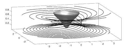
Figure 1: Streamlines highlighting the cyclonic vortex in the center of our convection cell. The conical eyewall is represented in shaded gray. Parameters: $\varepsilon=0.1$, $\Pr=0.1$, ${\rm E}=0.1$ and ${\rm Ra}=2\times 10^{4}$.

For the limited range of parameters considered in ODD17, the requirement for an eye to form is that the Reynolds number based on the peak inflow velocity must exceed ${\rm Re}\sim 37$. By contrast, at lower values of Re the flow is relatively diffusive, and so the negative azimuthal vorticity in the lower boundary layer cannot be advected upward to form an eyewall; hence the absence of an eye. To the best of our knowledge, this is the first attempt to establish a simple criterion for eye formation. However, ODD17 considered only a relatively small range of parameters, keeping the aspect ratio and Ekman number fixed and varying the Rayleigh number by a factor of only $30$. Here we revisit the entire problem and consider a much wider range of parameters. In particular, we present the results of a suite of over 150 numerical simulations in which the Rayleigh number, Ekman number and aspect ratio are all varied. The analysis of this suite of simulations shows that the conditions required for eye formation are more subtle than those suggested in ODD17.

II A Model Problem and Key Dimensionless Groups

Our model problem is the same as that in Oruba et al. (2017). It consists of the steady, laminar flow of a Boussinesq fluid in a closed, rotating cylinder of height $H$ and radius $R$, with aspect ratio $\varepsilon=H/R\ll 1$. We adopt cylindrical polar coordinates, $(r,\phi,z)$, with the upper and lower boundaries at $z=H$ and $z=0$. The motion is maintained by buoyancy with a prescribed heat flux between the two horizontal boundaries. The surfaces at $z=0$ and $r=R$ are no-slip boundaries, while the upper surface is taken to be stress free. This choice of boundary conditions is essential to our model as the vorticity generation in the bottom boundary layer is essential in the eyewall formation. It does not necessarily imply that counter-vortices (associated with a downward flow near the axis) are not possible under different configurations, such as for example a stress-free bottom boundary. However such structures would not feature a sharp eyewall as in the present model.

The choice of fixed heat flux boundary condition is motivated by our intention to model an elongated vortex: we want to drive a large-scale convective cell in an elongated domain. It is well known (e.g. Turner, 1973) that imposed flux boundary conditions will cause the convective cell to extend horizontally and fill the entire domain. This choice of boundary conditions is also the natural choice to model intense atmospheric vortices over the ocean, the main source of energy being the flux of water vapour from the ocean.

In the absence of convection there is an imposed, uniform temperature gradient of ${\rm d}T_{0}/{\rm d}z=-\beta$, and we write the temperature distribution in the presence of convection as $T=T_{0}(z)+\vartheta$. The governing equation for the temperature disturbance is then

$$\frac{{\rm D}\vartheta}{{\rm D}t}=\kappa\,\mbox{\boldmath$\nabla$}^{2}\vartheta+\beta u_{z}\,,$$ (1)

where $\kappa$ is the thermal diffusivity and $u_{z}$ the vertical velocity. We impose $\partial\vartheta/\partial z$ at $z=0$ and $z=H$ in order to maintain a constant axial heat flux, and the outer radial boundary is taken to be thermally insulating.

Let ${\bf\Omega}$ be the background rotation rate, and $\nu$, $\alpha$ and $\rho_{0}$ be the kinematic viscosity, expansion coefficient and mean density of the fluid. In a frame of reference which rotates with the boundaries $z=0$ and $r=R$, the governing equation of motion is then

$$\frac{{\rm D}{\bf u}}{{\rm D}t}=\,-{\mbox{\boldmath$\nabla$}}\left(p/\rho_{0}\right)\,+2\,{\bf u}\times{\bf\Omega}\,+\nu\mbox{\boldmath$\nabla$}^{2}{\bf u}\,-\alpha\vartheta{\bf g}\,,$$ (2)

where ${\bf u}$ is the solenoidal velocity field in the rotating frame, $p$ the departure from a hydrostatic pressure distribution, and $-\alpha\vartheta{\bf g}$ the buoyancy force per unit mass. The associated vorticity equation is

$$\frac{{\rm D}{\mbox{\boldmath$\omega$}}}{{\rm D}t}={\mbox{\boldmath$\omega$}}\cdot{\mbox{\boldmath$\nabla$}}{\bf u}\,+2\,{\bf\Omega}\cdot{\mbox{\boldmath$\nabla$}}{\bf u}\,+\nu\mbox{\boldmath$\nabla$}^{2}{\mbox{\boldmath$\omega$}}\,+\alpha{\bf g}\times\mbox{\boldmath$\nabla$}\vartheta\,,$$ (3)

where ${\mbox{\boldmath$\omega$}}={\mbox{\boldmath$\nabla$}}\times{\bf u}$.

Since we restrict ourselves to axisymmetric velocity fields it is convenient to decompose ${\bf u}$ into poloidal, ${\bf u}_{p}=(u_{r},0,u_{z})$, and azimuthal, ${\bf u}_{\phi}=(0,\Gamma/r,0)$, components, in which $\mbox{\boldmath$\nabla$}\cdot{\mbox{\bf u}}_{p}=0$ and $\Gamma=ru_{\phi}$ is the angular momentum density in the rotating frame. The azimuthal component of (2) and (3) then becomes evolution equations for $\Gamma$ and $\omega_{\phi}=\left(\nabla\times{\mbox{\bf u}}_{p}\right)\cdot\mbox{\boldmath$\hat{e}$}_{\phi}$,

$$\displaystyle\frac{{\rm D}}{{\rm D}t} \left(\Gamma+\Omega r^{2}\right)=\,\nu\mbox{$\nabla_{\star}^{2}$}{\Gamma}$$ (4)

$$\displaystyle\frac{{\rm D}}{{\rm D}t} \left(\frac{\omega_{\phi}}{r}\right)=\frac{\partial}{\partial z}\left(\frac{\Gamma^{2}}{r^{4}}\right)+\frac{2\,\Omega}{r}\frac{\partial u_{\phi}}{\partial z}-\frac{\alpha g}{r}\,\frac{\partial\vartheta}{\partial r}+\frac{\nu}{r^{2}}\mbox{$\nabla_{\star}^{2}$}\left(r\omega_{\phi}\right)\,,$$ (5)

where $\nabla_{\star}^{2}$ is the Stokes operator,

$$\mbox{$\nabla_{\star}^{2}$}=r\frac{\partial}{\partial r}\left(\frac{1}{r}\frac{\partial}{\partial r}\right)+\frac{\partial^{2}}{\partial z^{2}}\,.$$ (6)

(See, for example, Davidson, 2013, for a derivation of equations (4) and (5)). The Stokes stream-function, defined by $\mbox{\bf u}_{p}=\mbox{\boldmath$\nabla$}\times\left[\left(\psi/r\right)\mbox{\boldmath$\hat{e}$}_{\phi}\right]$, can be determined from $\omega_{\phi}$ by inverting the Poisson equation $r\omega_{\phi}=-\mbox{$\nabla_{\star}^{2}$}\psi$. It follows that the two scalar fields $\Gamma$ and $\omega_{\phi}$ uniquely determine the instantaneous velocity distribution, and so the governing equations for our model system are (1), (4) and (5).

The dimensionless control parameters normally used to investigate the stability of this kind of rotating convection are

$$\varepsilon=\frac{H}{R}\,,\qquad\Pr=\frac{\nu}{\kappa}\,,\qquad{\rm E}=\frac{\nu}{\Omega H^{2}}\,,\qquad{\rm Ra}=\frac{\alpha g\beta H^{4}}{\nu\kappa}\,,$$ (7)

where $\Pr$ is the Prandtl number, ${\rm E}$ the Ekman number and ${\rm Ra}$ the Rayleigh number. However, since we are looking at fully-developed flow, rather than the stability of a static equilibrium, we shall find it convenient to work with an alternative set of dimensionless parameters. Let us introduce the velocity scale $V=(\alpha g\beta)^{1/2}H$, which will turn out to be characteristic of the actual fluid velocity. Then an alternative, if equivalent, set of dimensionless control parameters is

$$\varepsilon=\frac{H}{R}\,,\qquad\Pr=\frac{\nu}{\kappa}\,,\qquad{\rm Re}=\frac{VH}{\nu}\,,\qquad{\rm Ro}=\frac{V}{\Omega H}\,,$$ (8)

where ${\rm Re}$ and ${\rm Ro}$ are characteristic Reynolds and Rossby numbers. One potential advantage of (8) over (7) is that, if we are allowed to take $V$ as truly representative of fluid velocity, then ${\rm Re}$ and ${\rm Ro}$ have a simple physical interpretation in terms of the relative dynamical balance in (2). The dimensionless control parameters (8) indeed naturally enter the non-dimensional form of equations (1) and (2) using $H$, $V$ and $\beta H$ as units of length, speed and temperature, which provides

$$\frac{{\rm D}\vartheta^{\star}}{{\rm D}t^{\star}} = {\rm Re}^{-1}\,{\Pr}^{-1}\,\mbox{\boldmath$\nabla$}^{2}\vartheta^{\star}+u_{z}^{\star}$$ (9)

$$\frac{{\rm D}{\bf u^{\star}}}{{\rm D}t^{\star}} = \,-{\mbox{\boldmath$\nabla$}}\pi\,+2\,{\rm Ro}^{-1}\,{\bf u^{\star}}\times{\mbox{\boldmath$\hat{e}$}_{z}}\,+{\rm Re}^{-1}\,\mbox{\boldmath$\nabla$}^{2}{\bf u^{\star}}\,+\vartheta^{\star}{\mbox{\boldmath$\hat{e}$}_{z}}\,,$$ (10)

where a ^⋆ denotes dimensionless quantities. Moreover, ODD17 have already noted the importance of ${\rm Re}$ as a control parameter for the appearance of an eye. Of course, it is easy to go from (7) to (8), with ${\rm Ro}={\rm Ra}^{1/2}{\rm E}\Pr^{-1/2}$ and ${\rm Re}={\rm Ra}^{1/2}\Pr^{-1/2}$.

The eyewall tends to be confined to the region $r<H$ and, as noted above, the dynamics in the vicinity of the eyewall tends to be quite different to be that in the bulk of the vortex. In particular, although the Coriolis and buoyancy forces are of the same order of magnitude as inertia in the bulk, they are negligible near the eyewall where inertia is particularly high. Consequently, for diagnostic purposes, we shall find it convenient to introduce the following local definitions of ${\rm Re}$ and ${\rm Ro}$. Let $u_{\phi,m}$ be the maximum azimuthal velocity on the surface $r=H$, and $u_{r,\delta}$ be the magnitude of the radial velocity at location $\left(r=H,z=\delta\right)$, where $z=\delta$ is the upper edge of the bottom boundary layer, defined at a given radius as the point where negative azimuthal vorticity $\omega_{\phi}$ in the boundary layer becomes positive. We then define local values of ${\rm Re}$ and ${\rm Ro}$ in the vicinity of the eyewall as ${\rm Re}_{r}=u_{r,\delta}H/\nu$, ${\rm Re}_{\phi}=u_{\phi,m}H/\nu$, ${\rm Ro}_{r}=u_{r,\delta}/(\Omega H)$ and ${\rm Ro}_{\phi}=u_{\phi,m}/(\Omega H)$. More generally, we introduce local values of ${\rm Ro}_{r}(r)$ and ${\rm Ro}_{\phi}(r)$ for any radius, based on the local values of $u_{r,\delta}(r)$ and $u_{\phi,m}(r)$.

The numerical values of the dimensionless control parameters used in our suite of numerical simulations are tabulated in the Appendix, along with the corresponding values of ${\rm Ro}$, ${\rm Re}$, ${\rm Ro}_{r}$, ${\rm Re}_{r}$ and the magnitude of the maximum downward velocity on the axis, $|{\rm u}_{z}|^{\rm max}_{\rm r=0}$. The dimensionless parameters listed in (7) are restricted to the ranges $0.1<\varepsilon<0.3$, $0.1<\Pr<1$, $0.07<{\rm E}<0.4$ and $10^{3}<{\rm Ra}<4.5\times 10^{4}$. These correspond to values of ${\rm Re}$, ${\rm Ro}$ and ${\rm Re}_{r}$ of $45<{\rm Re}<616$, $4.5<{\rm Ro}<124$ and $6<{\rm Re}_{r}<188$. A zero entry for $|{\rm u}_{z}|^{\rm max}_{\rm r=0}$ in the table indicates that no eye formed in that simulation, while a non-zero value provides a measure of the strength of the eye.

There are 157 simulations in total. Each numerical experiment comprises an initial value problem which is run until a steady state is reached. We solve equations (1), (4) and (5) using second-order finite differences with an implicit second-order backward differentiation in time. The grid resolution is $1000$ radial $\times 500$ axial cells and grid resolution studies were performed to ensure convergence.

The strength and shape of the eye depends on the parameter regime, see table 1, and figure 2.

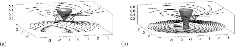
Figure 2: Similar representation as Figure 1 for different choices of parameters: (a) $\varepsilon=0.1$, $\Pr=0.1$, ${\rm E}=0.15$ and ${\rm Ra}=1\times 10^{4}\,,$ (b) $\varepsilon=0.1$, $\Pr=1$, ${\rm E}=0.1$ and ${\rm Ra}=4.5\times 10^{4}\,.$

III General Flow Structure and Scaling Laws

As a prelude to our discussion of the conditions under which eyes form, it is useful to consider the general structure of the flow and the scaling laws for the velocity field. In order to illustrate some of the more general features of the flow, let us start by considering the specific (though typical) case in which the control parameters are $\varepsilon=0.1$, $\Pr=0.1$, ${\rm E}=0.1$ and ${\rm Ra}=2\times 10^{4}$, or equivalently ${\rm Re}=447$ and ${\rm Ro}=44.7$. The Reynolds number and Rossby number in the vicinity of the eyewall are ${\rm Re}_{r}=176$ and ${\rm Ro}_{\phi}=30$.

The Stokes stream-function and radial variations of ${\rm Ro}_{r}(r)$ and ${\rm Ro}_{\phi}(r)$ for this case are shown in Figure 3, and it is evident that an eye has formed near the axis. Note that ${\rm Ro}_{\phi}(r)$, and hence $u_{\phi}$, rises rapidly as we approach the eyewall, which is a consequence of approximate angular momentum conservation in the incoming flow. The local value of ${\rm Ro}_{\phi}$ near the eye is therefore large and background rotation has no direct influence on the flow in this region. Note also that $u_{\phi,m}$ is smaller than $u_{r,\delta}$ in the bulk of the vortex, but that $u_{\phi,m}$ exceeds $u_{r,\delta}$ near the eyewall.

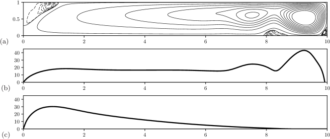
Figure 3: (a) The Stokes stream-function. (b) The radial variations of ${\rm Ro}_{r}(r)$ and (c) ${\rm Ro}_{\phi}(r)$. Parameters: $\varepsilon=0.1$, $\Pr=0.1$, ${\rm E}=0.1$ and ${\rm Ra}=2\times 10^{4}$.

Figure 4 shows the corresponding distributions of azimuthal velocity, $u_{\phi}$, angular momentum, $\Gamma$, and total temperature, $T=T_{0}(z)+\vartheta$. The intensification of $u_{\phi}$ by the inward advection of angular momentum is evident in Figure 4(a), while  4(b) shows that, in the region immediately to the right of the eye, the contours of constant angular momentum are roughly aligned with the streamlines, indicative of ${\rm D}{\Gamma}/{{\rm D}t}\simeq 0$. This is to be expected from (4), given that the background rotation is locally weak and diffusion is largely restricted to the boundary layer and the eyewall. This figure also shows a substantial region of negative $u_{\phi}$ (anti-cyclonic rotation) at large radius, something that is also noted in ODD17 and is observed in tropical cyclones. From Figure 4(c) we see that the poloidal flow sweeps hot fluid upward near the axis and cold fluid downward and inwards at $r=R$. The resulting negative radial gradient in temperature drives the main poloidal vortex, ensuring that it has positive azimuthal vorticity in accordance with equation (5).

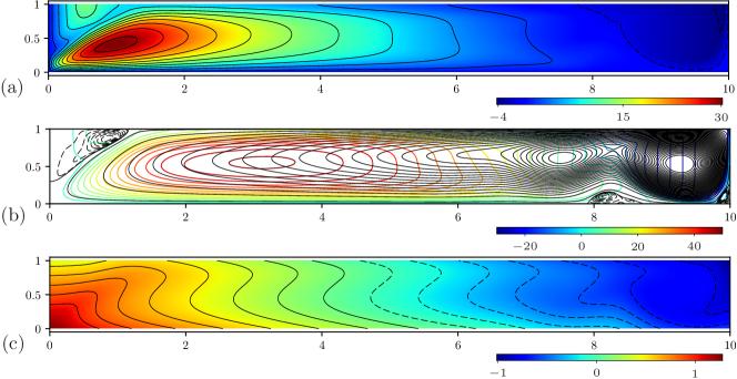
Figure 4: Colour maps of: (a) the azimuthal velocity, $u_{\phi}$, (b) the angular momentum, $\Gamma$, superimposed on the stream-function, and (c) the total temperature $T=T_{0}(z)+\vartheta$. Parameters: $\varepsilon=0.1$, $\Pr=0.1$, ${\rm E}=0.1$ and ${\rm Ra}=2\times 10^{4}$.

The structure of the eyewall is particularly evident in Figure 5, which shows the distribution of azimuthal vorticity, $\omega_{\phi}/r$. It is clear that there are intense levels of azimuthal vorticity in the vicinity of the eyewall, and indeed it is natural to define the eyewall as the conical annulus of strong negative azimuthal vorticity. The eyewall then separates the eye from the primary vortex. Note also that an intense region of negative azimuthal vorticity has built up in the lower boundary layer, and it is shown in ODD17 that this is the ultimate source of the eyewall vorticity. A region of strong positive azimuthal vorticity is also evident between the lower boundary and the eyewall. As noted in ODD17, this is a local effect caused by the source term $\mbox{\boldmath$\nabla$}\cdot\left[\left(\Gamma^{2}/r^{4}\right)\mbox{\boldmath$\hat{e}$}_{z}\right]$ in (5), which is particularly large near the base of the eyewall. However, since this source term takes the form of a flux it cannot contribute to the mean azimuthal vorticity in the eyewall (see ODD17).

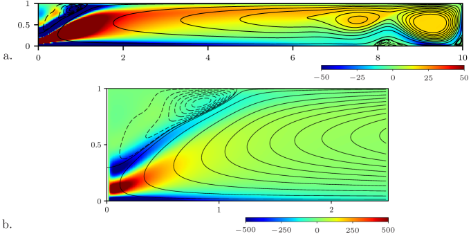
Figure 5: Colour map of $\omega_{\phi}/r$ superimposed on the streamlines. (a) Full flow field. (b) Flow in the inner quarter of the domain. Parameters: $\varepsilon=0.1$, $\Pr=0.1$, ${\rm E}=0.1$ and ${\rm Ra}=2\times 10^{4}$.

The general structure of the flow shown in Figures 3, 4 and 5 is typical of all of our simulations which exhibit an eye. However, the scaling of the various velocity components and the characteristic thickness of the bottom boundary layer depends on the precise values of the control parameters. Let us start with some observations about the thickness of the bottom boundary layer.

Figure 6 shows $\delta^{\star}=\delta/H$, the dimensionless boundary-layer thickness, evaluated at mid radius, $r=R/2$, and plotted as a function of ${\rm Ro}$ in Figure 6(a) and ${\rm E}$ in Figure 6(b). The results of all 87 numerical simulations for $\varepsilon=0.1$ and $\Pr=0.1$ are shown. It is clear from Figure 6(a) that there are two regimes. For ${\rm Ro}<25$ we see that $\delta$ is an increasing function of ${\rm Ro}$, while for ${\rm Ro}>30$ there is evidence that $\delta$ saturates at approximately $H/4$. We shall see shortly that these two distinct regimes also manifest themselves in the scaling laws for the velocity field, with a transition at around ${\rm Ro}\sim 25$. Figure 7 shows the same data, but for the location $r=H$. The boundary layer is now much thinner and there is some suggestion in Figure 7(b) that $\delta^{\star}\sim{\rm E}^{1/2}$. This, in turn, suggests that the boundary layer at $r=H$ scales approximately as $\delta\sim(\nu/\Omega)^{1/2}$, as in a conventional Ekman layer.

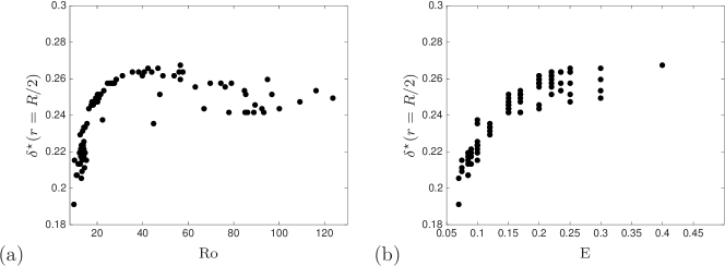
Figure 6: The dimensionless boundary-layer thickness at mid radius, $\delta^{\star}(r=R/2)$, as a function of: (a) ${\rm Ro}$, and (b) ${\rm E}$.

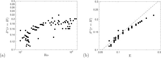
Figure 7: The dimensionless boundary-layer thickness at $r=H$, $\delta^{\star}(r=H)$, as a function of: (a) ${\rm Ro}$, and (b) ${\rm E}$. The dashed line corresponds to $\delta^{\star}\sim{\rm E}^{1/2}$.

We now consider the velocity ratio $u_{\phi,m}/u_{r,\delta}$. A preliminary analysis of the data indicates that this velocity ratio scales approximately as $u_{\phi,m}/u_{r,\delta}\sim{\rm E}^{-1/2}$, a scaling which is highlighted on Figure 8, together with the remaining Rossby number dependence.

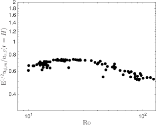
Figure 8: The velocity ratio ${\rm E}^{1/2}u_{\phi,m}/u_{r,\delta}$ at $r=H$ as a function of ${\rm Ro}$.

Regarding the scaling laws for the velocity field, it is instructive to integrate equation (2) once around a closed streamline. The inertial, pressure and Coriolis terms all drop out and we are left with the simple expression

$$\nu\oint\mbox{\boldmath$\nabla$}^{2}{\bf u}\cdot{\rm d}{\bf r}=\oint\left(\alpha\vartheta\mbox{\bf g}\right)\cdot{\rm d}{\bf r}\,.$$ (11)

This represents an energy balance for a fluid particle as it is swept once around a closed streamline. In particular, it represents the balance between the viscous dissipation of energy and the work done on the fluid particle by the buoyancy force as the particle is carried around a streamline. For those cases in which the dissipation occurs primarily in the bottom boundary layer, this yields the estimate

$$\nu\frac{u_{r,\delta}}{\delta^{2}}R\sim\alpha g\beta H^{2}=V^{2}\,.$$ (12)

(We have taken advantage of the fact that $u_{\phi,m}/u_{r,\delta}\leq 1$ at most radii to omit the contribution from $u_{\phi}$.) If, in addition, we adopt the suggestion of Figure 7(b) that the boundary layer thickness scales as $\delta\sim(\nu/\Omega)^{1/2}$, as in an Ekman layer, then we conclude that

$$\frac{u_{r,\delta}}{V}\sim\frac{V}{\Omega R}=\varepsilon{\rm Ro}\,.$$ (13)

However, this estimate holds only when there is a well-developed boundary layer on the lower surface in which $\delta$ is much thinner than $H$. If the boundary layer grows to be of order $H$, on the other hand, the dissipation will be distributed throughout the bulk of the fluid and we would expect a different scaling law to hold. Figure 6(a) tentatively suggests that scaling (13) might be appropriate for ${\rm Ro}<25$, but not for ${\rm Ro}>30$.

Figure 9 shows: (a) $u_{r,\delta}/V$, (b) $u_{\phi,m}/V$, and (c) ${\rm E}^{1/2}u_{\phi,m}/V$, all evaluated at $r=H$ and plotted against ${\rm Ro}$. The data in Figure 9(a) supports the idea that there are two regimes, with a transition at around ${\rm Ro}\sim 25$. Moreover, for ${\rm Ro}<25$ there is some evidence in support of (13), while for ${\rm Ro}>25$ the radial velocity saturates at $u_{r,\delta}\sim V$. There is considerably more scatter in Figure 9(b), which shows $u_{\phi,m}/V$ as a function of ${\rm Ro}$. However, we have already noted that $u_{\phi,m}/u_{r,\delta}\sim{\rm E}^{-1/2}$ at $r=H$ and so Figure 9(c) shows the same data in the form ${\rm E}^{1/2}u_{\phi,m}/V$. The data is now reasonably well collapsed and again there is clear evidence of a transition in regimes at around ${\rm Ro}\sim 25$.

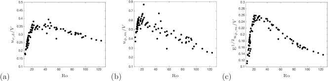
Figure 9: (a) $u_{r,\delta}/V$ at $r=H$ as a function of ${\rm Ro}$. (b) $u_{\phi,m}/V$ versus ${\rm Ro}$. (c) ${\rm E}^{1/2}u_{\phi,m}/V$ versus ${\rm Ro}$.

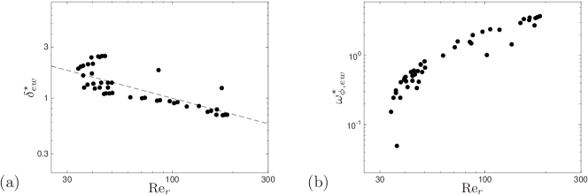
Figure 10: Variation of (a) the width of the eyewall as measured by $\delta^{\star}_{ew}$ (the dashed line indicates a ${\rm Re}_{r}^{-1/2}$ scaling) and (b) the peak azimuthal vorticity in the eyewall $\omega^{\star}_{\phi,ew}\,,$ both as a function of the Reynolds number ${\rm Re}_{r}\,.$

Let us finally consider the thickness and strength of the vorticity in the eyewall. We define the width of the eyewall $\delta^{\star}_{ew}$ as the horizontal extent of the negative azimuthal vorticity at the height of the eye center $z_{eye}$ (we restrict ourselves here to cases in which an eye was observed). It is to be expected that the width of the eyewall $\delta^{\star}_{ew}$ depends on the ratio of advection along the eyewall to that of cross-stream diffusion. This appears to be well supported by Figure 10(a). Indeed the width of the eyewall appears to scale as ${\rm Re}_{r}^{-1/2}$ as anticipated from a balance of streamwise advection and cross-stream diffusion. The strength of the vorticity in the eyewall can be estimated as $\omega^{\star}_{\phi,ew}=-{\rm min}(\omega^{\star}_{\phi}(r,z_{eye}))\,.$ Figure 10(b) shows the increase of $\omega^{\star}_{\phi,ew}$ as the Reynolds number ${\rm Re}_{r}$ is increased. The nature of the supercritical bifurcation to an eye will be the object of the next section.

IV The Transition to an Eye

It was noted in ODD17 that, for the limited set of cases examined, an eye would not form when ${\rm Re}_{r}<37$. The reason is that the flow is then too diffusive for the boundary layer vorticity to be advected up in the bulk for the flow, and without this boundary layer vorticity, an eyewall cannot form. We now revisit this transition from no eye to an eye, focussing exclusively on the flow in the region $r\leq H$. We shall use as a measure of the strength of the eye the magnitude of the maximum downward velocity on the axis, $|{\rm u}_{z}|^{\rm max}_{\rm r=0}$. The value of $|{\rm u}_{z}|^{\rm max}_{\rm r=0}$ observed in each simulation is tabulated in the Appendix, with a zero entry for $|{\rm u}_{z}|^{\rm max}_{\rm r=0}$ in the tables indicating that no eye formed in that simulation.

Figure 11 shows $|{\rm u}_{z}|^{\rm max}_{\rm r=0}$ plotted as a function of (a) the measured ${\rm Re}_{r}$ and (b) the controlled ${\rm Re}$ for different values of ${\rm E}$. (Both $\Pr$ and $\varepsilon$ are held fixed at $\varepsilon=0.1$ and $\Pr=0.1$.) There is indeed a supercritical bifurcation to an eye at around ${\rm Re}_{r,crit}\sim 40$, but there is also clear evidence that the critical Reynolds number, ${\rm Re}_{r,crit}$, depends on ${\rm E}$, with ${\rm Re}_{r,crit}$ varying from around $34$ up to a maximum of $50$. Considering the control parameter ${\rm Re}$ yields somewhat more scatter in the plot of $|{\rm u}_{z}|^{\rm max}_{\rm r=0}$ versus ${\rm Re}$, but the general trend is similar, with a supercritical bifurcation in the range $110<{\rm Re}_{crit}<170$.

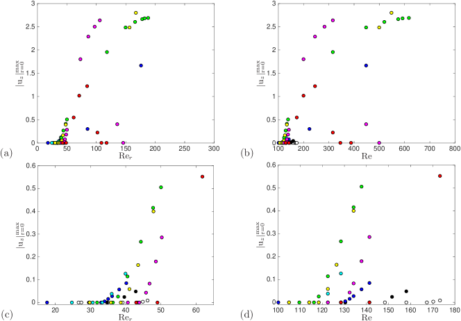
Figure 11: Bifurcation diagrams of $|{\rm u}_{z}|^{\rm max}_{\rm r=0}$ versus Reynolds number, with the bottom panels focused on the region of the bifurcation. The Ekman number is allowed to vary, but $\Pr$ and $\varepsilon$ are fixed at $\Pr=\varepsilon=0.1$. The colour code indicates the values of ${\rm E}$, with ${\rm E}=0.085$ (white), ${\rm E}=0.090$ (black), ${\rm E}=0.10$ (blue), ${\rm E}=0.12$ (light blue), ${\rm E}=0.15$ (green), ${\rm E}=0.17$ (yellow), ${\rm E}=0.20$ (pink), ${\rm E}=0.22$ (red). (a), (c) $|{\rm u}_{z}|^{\rm max}_{\rm r=0}$ plotted as a function of ${\rm Re}_{r}$. (b), (d) $|{\rm u}_{z}|^{\rm max}_{\rm r=0}$ plotted as a function of ${\rm Re}$.

The degree to which the critical Reynolds numbers ${\rm Re}_{r,crit}$ and ${\rm Re}_{crit}$ vary with ${\rm E}$, $\Pr$ and $\varepsilon$ is explored in Figure 12. Panels (a) and (b) show the dependency on ${\rm E}$, (c) and (d) the dependency on $\Pr$, and (e) and (f) the dependency on $\varepsilon$. Interestingly, there is an optimum Ekman number for eye formation in the sense that ${\rm Re}_{r,crit}$ and ${\rm Re}_{crit}$ both exhibit minima. This minimum is around ${\rm E}\sim 0.1$ for ${\rm Re}_{r,crit}$ and ${\rm E}\sim 0.15$ for ${\rm Re}_{crit}$. Note also that no eyes are observed when ${\rm E}$ falls below $0.07$ or rises above $0.25$, as indicated by the grey areas in panels (a) and (b). We shall return to this observation shortly. There is also an optimal value of $\varepsilon$ for eye formation, at around $\varepsilon\sim 0.15-0.2$, with a complete absence of eyes for $\varepsilon>0.3$ (at least for the range of parameters considered here). This suggests that a low aspect ratio is important for eye formation in this particular model problem.

The dependency of ${\rm Re}_{r,crit}$ and ${\rm Re}_{crit}$ on $\Pr$ is more complicated. While ${\rm Re}_{r,crit}$ is only weakly dependent on $\Pr$, ${\rm Re}_{crit}$ displays a marked dependency on $\Pr$, with ${\rm Re}_{crit}$ rising sharply as $\Pr$ is increased. However, since ${\rm Re}_{r,crit}$ is evaluated near the eyewall, and ${\rm Re}_{crit}$ is a global quantity, we interpret the left-hand panel as indicating that $\Pr$ plays little or no role in the local dynamics of eye formation. The apparent dependency on $\Pr$ in the right-hand panel is then a manifestation of the fact that the global flow structure, and hence the ratio ${\rm Re}_{r}/{\rm Re}$, is a function of $\Pr$.

While there are clearly lower bounds on ${\rm Re}_{r,crit}$ and ${\rm Re}_{crit}$ for eye formation, it is natural to ask if other conditions need to be satisfied. For example, the absence of eyes in Figure 12 for ${\rm E}<0.07$ and ${\rm E}>0.25$ is intriguing. This is explored in Figure 13, which presents scatter plots (or phase diagrams) of (a) ${\rm E}$ versus ${\rm Re}_{r}$ and (b) ${\rm E}$ versus ${\rm Re}$. In both cases the filled circles indicate the absence of an eye and the empty circles the presence of an eye. As in Figure 11, $\Pr$ and $\varepsilon$ are both held fixed at $\Pr=\varepsilon=0.1$. A more complex picture now emerges, with both upper and lower limits on ${\rm E}$ for eye formation, in addition to the lower bounds on ${\rm Re}_{r,crit}$ and ${\rm Re}_{crit}$.

The upper limit on ${\rm E}$ is to be expected from a consideration of global dynamics. That is to say, the presence of an eye rests on the formation of an eyewall, and this, in turn, requires the presence of a thin Ekman-like boundary layer surrounding the axis within which the fluid spirals inward. If ${\rm E}$ is too large, then the Coriolis force acting in the bulk is unable to establish such a thin boundary layer in the face of strong viscous forces.

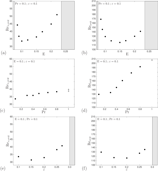
Figure 12: Critical Reynolds numbers ${\rm Re}_{r,crit}$ (left column) and ${\rm Re}_{crit}$ (right column). The grey areas denote an absence of an eye. The diamonds correspond to a hysteretic case.

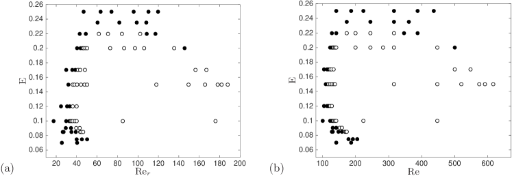
Figure 13: Scatter plots of (a) ${\rm E}$ versus ${\rm Re}_{r}$ and (b) ${\rm E}$ versus ${\rm Re}$. The filled circles indicate the absence of an eye and the empty circles the presence of an eye. Both $\Pr$ and $\varepsilon$ are held fixed at $\Pr=\varepsilon=0.1$.

V Discussion

Let us now pull together the results of the section IV and summarise the conditions under which an eye is likely to form, at least in the particular model system investigated here. This is summarised in cartoon fashion in Figure 14 as a phase diagram of ${\rm E}$ versus ${\rm Re}$, with $\Pr$ and $\varepsilon$ both held fixed.

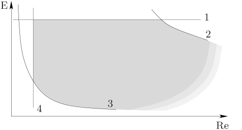
Figure 14: Schematic structure of the phase diagram for the appearance of eyes in the model system considered in this paper. Eyes are not expected to form outside the shaded region limited by the four curves shown. Extension of this domain to the right of this figure is so far unexplored.

We suggest that the regime in which eyes are expected to form is limited by four curves. Line $4$ is the lower bound on ${\rm Re}$ identified by ODD17, while line $1$ is the upper bound on ${\rm E}$ discussed above. Curves $2$ and $3$ are both of the form

$${\rm E}={\rm Ro}_{crit}/{\rm Re}\,,$$ (14)

and represent upper and lower bounds on the Rossby number. While there is clear evidence in favour of lines $1$ and $4$ in Figure 13, there is only moderate support for lines $2$ and $3$. However, upper and lower bounds on ${\rm Ro}$, as expressed by (14), are conceptually necessary, as we now discuss.

The idea behind an upper bound on ${\rm Ro}$ is the assertion that the Coriolis force is essential for shaping the global flow pattern into a configuration favourable to eye formation. In particular, an appreciable Coriolis force acting on the bulk of the vortex is required to induce an Ekman-like boundary layer on the lower surface, without which an eyewall cannot form. So the Coriolis force cannot be significantly smaller than either the viscous or the inertial forces in the main body of the vortex. The restriction that the Coriolis force out-ways the viscous stresses leads to line $1$, as discussed above, while the requirement that it is at least as large as the inertial forces places an upper bound on ${\rm Ro}$ and yields line $2$.

The lower bound on ${\rm Ro}$ stems from the fact that the local dynamics of eye formation occurs without any significant local influence from the buoyancy or Coriolis forces, as emphasised in ODD17. Indeed, it is essential that ${\rm Ro}_{\phi}$ is large (or at least greater than unity) at $r=H$, as otherwise quasi-geostrophy near the axis would prevent the lower boundary separating to form a conical shear layer, and hence prevent the formation of an eyewall. So we require ${\rm Ro}_{\phi}>1$ for an eye to form and this, in turn, suggests a lower bound on ${\rm Ro}$ in the bulk of the flow, thus leading to curve $3$. Certainly, it is noticeable that in tropical cyclones ${\rm Ro}_{\phi}$ near the eyewall is invariably significantly larger than unity.

In summary, then, there is clear supporting evidence for lines $1$ and $4$ in Figure 13, and also some support for lines $2$ and $3$. Never-the-less, conceptually consistency requires an upper bound on ${\rm Ro}$ and a lower bound on ${\rm Ro}_{\phi}$ for eye formation, at least for the particular model system considered here.

It is interesting to consider the applicability of our simplified model to large-scale cyclonic vortices occurring in atmospheric flows, such as tropical cyclones. Of course, one must be cautious in such attempts, and it is important to stress that certain essential characteristics of atmospheric vortices have been dropped in the present model. These include vertical stratification, spatially varying and anisotropic eddy viscosity, as well as latent heat release due to water vapour condensation. However, most large-scale atmospheric vortices (tropical cyclones, medicanes, polar lows) exhibit an eye, which may be related to the eye in our simplified model.

The appropriate level of turbulent diffusion required to model a tropical cyclone is a poorly constrained quantity (Rotunno et al., 2009). It is most certainly non-uniform in space and anisotropic. For the sake of simplicity, we could estimate an order of magnitude for the relevant Ekman number, based on eddy viscosities in the range $1\rightarrow 10^{3}$ m².s^-1 and latitudes varying between some $10^{\circ}$ and $30^{\circ}$. This yields an estimate of the Ekman number in the range $10^{-4}\rightarrow 0.2\,.$ Dropwindsonde observations in actual tropical cyclones indicate that the inward radial flow above the boundary layer and at a radius close to the eye is smaller by a factor about 10 than the azimuthal flow at the same location (Giammanco et al., 2013). This suggests, via the ratio $u_{\phi,m}/u_{r,\delta}\sim{\rm E}^{-1/2}\,,$ an effective Ekman number of the order of $10^{-2}$. Such estimates happen to be consistent with estimates of the eddy viscosity above the boundary layer as well as with observations of the boundary layer thickness in actual tropical cyclones (Bryan et al., 2017). Reynolds and Rossby number estimates may then be constructed on the basis of such eddy viscosity orders of magnitude and in situ measurements of the inward radial flow (typically $5$ m.s^-1) and azimuthal flow (typically $50$ m.s^-1). These estimates suggest ${\rm Re}_{r}$ lies in the range $10^{2}\rightarrow 10^{5}$ and ${\rm Ro}_{\phi}$ in the range $70\rightarrow 220$, which include the parameter range covered by our numerical study. Another encouraging observation concerns the tilt of the eyewall. Airborne Doppler radar data indicate that the eyewall in hurricanes is on average characterised by a tilt angle of some $45^{\circ}$ (Hazelton and Hart, 2013; Stern et al., 2014), comparable to the tilt produced in the simplified model (see Figure 5). These observations may indicate that the fluid mechanics model presented here, albeit simplified, is not irrelevant to some aspects of the dynamics of tropical cyclones, and could capture some of the important physical mechanisms.

We should stress however the important distinction between the large-scale vortices discussed here and elongated atmospheric vortices, such as tornadoes or dust devils. These tornado-like vortices have an inversed aspect ratio compared to our model. They do exhibit an eye-like structure, possibly associated with vortex breakdown. However, this breakdown is characterised by a much steeper wall (see for example Fiedler, 1994; Nolan, 2005; Rotunno, 2013). Such phenomena correspond to a different configuration (both in terms of aspect ratio and of controlling parameters), and our model is not relevant to such flows. Rather, we intend to model atmospheric vortices characterised by a large horizontal scale.

VI Conclusions

We have extended the study of ODD17, establishing scaling laws for the flow and mapping out the conditions under which an eye will form. We have shown that, to leading order, the velocity scales on $V=(\alpha g\beta)^{1/2}H$, and that the two most important parameters controlling the dynamics are ${\rm Re}={VH}/{\nu}$ and ${\rm Ro}={V}/\left(\Omega H\right)$, with $\Pr$ and $\varepsilon$ playing an important but secondary role. We have also shown that the criterion for eye formation in ODD17 is too simplistic, and that upper and lower bounds on ${\rm Ro}$, as well as an upper bound on ${\rm E}$, must be taken into consideration.

Appendix A Numerical results

The following table presents the controlling parameters ${\rm Ra}$, ${\rm Ro}$, ${\rm Re}$, and the diagnostic quantities ${\rm Ro}_{r}$, ${\rm Re}_{r}$ and $|{\rm u}_{z}|^{\rm max}_{\rm r=0}$ in our numerical database.

Table Ia: Numerical results.

${\rm Ra}$	${\rm Ro}$	${\rm Re}$	${\rm Ro}_{r}$	${\rm Re}_{r}$	$|{\rm u}_{z}|^{\rm max}_{\rm r=0}$
$\varepsilon=0.1$  ${\rm E}=0.07$  $\Pr=0.1$
2000	9.90	141.42	1.80	25.72	0
3500	13.10	187.08	2.84	40.56	0
$\varepsilon=0.1$  ${\rm E}=0.075$  $\Pr=0.1$
3200	13.42	178.89	2.99	39.82	0
3700	14.43	192.35	3.38	45.00	0
4200	15.37	204.94	3.77	50.23	0
$\varepsilon=0.1$  ${\rm E}=0.085$  $\Pr=0.1$
1650	10.92	128.45	2.26	26.56	0
1700	11.08	130.38	2.33	27.36	0
2200	12.61	148.32	2.96	34.86	0
2500	13.44	158.11	3.33	39.19	0
2800	14.22	167.33	3.69	43.46	0
2900	14.47	170.29	3.81	44.87	0.0023
3000	14.72	173.21	3.93	46.25	0.0076
$\varepsilon=0.1$  ${\rm E}=0.09$  $\Pr=0.1$
1700	11.73	130.38	2.66	29.55	0
2000	12.73	141.42	3.12	34.69	0
2300	13.65	151.66	3.57	39.63	0.0230
2500	14.23	158.11	3.86	42.87	0.0486
$\varepsilon=0.1$  ${\rm E}=0.1$  $\Pr=0.1$
1000	10.00	100.00	1.77	17.66	0
1500	12.25	122.47	2.97	29.71	0
1650	12.85	128.45	3.30	32.96	0
1700	13.04	130.38	3.40	34.01	0.0041
1750	13.23	132.29	3.51	35.06	0.0150
1800	13.42	134.16	3.61	36.10	0.0281
1900	13.78	137.84	3.81	38.14	0.0563
2000	14.14	141.42	4.01	40.15	0.0840
5000	22.36	223.61	8.53	85.28	0.3024
20000	44.72	447.21	17.61	176.10	1.6691
$\varepsilon=0.1$  ${\rm E}=0.1$  $\Pr=0.3$
2000	8.16	81.65	1.90	18.95	0
4000	11.55	115.47	3.03	30.33	0
5000	12.91	129.10	3.46	34.56	0
5500	13.54	135.40	3.64	36.44	0.0168
6000	14.14	141.42	3.82	38.20	0.0699
8000	16.33	163.30	4.43	44.26	0.3565
9000	17.32	173.21	4.68	46.83	0.4369

Table Ib: Numerical results (cont.)

${\rm Ra}$	${\rm Ro}$	${\rm Re}$	${\rm Ro}_{r}$	${\rm Re}_{r}$	$|{\rm u}_{z}|^{\rm max}_{\rm r=0}$
$\varepsilon=0.1$  ${\rm E}=0.1$  $\Pr=0.4$
6000	12.25	122.47	2.98	29.82	0
8000	14.14	141.42	3.50	34.96	0
8300	14.40	144.05	3.57	35.66	0
8450	14.53	145.34	3.60	35.99	0.0016
8600	14.66	146.63	3.63	36.33	0.0080
8800	14.83	148.32	3.68	36.78	0.0203
9000	15.00	150.00	3.72	37.22	0.0359
$\varepsilon=0.1$  ${\rm E}=0.1$  $\Pr=0.5$
6000	10.95	109.54	2.42	24.24	0
8000	12.65	126.49	2.86	28.58	0
10000	14.14	141.42	3.23	32.34	0
11500	15.17	151.66	3.49	34.88	0
12000	15.49	154.92	3.57	35.68	0
13000	16.12	161.25	3.72	37.21	0.0246
15000	17.32	173.21	3.99	39.85	0.6992
$\varepsilon=0.1$  ${\rm E}=0.1$  $\Pr=0.65$
16000	15.69	156.89	3.29	32.90	0
18000	16.64	166.41	3.51	35.09	0
19000	17.10	170.97	3.61	36.13	0
21000	17.97	179.74	3.81	38.11	0.0523
21250	18.08	180.81	3.83	38.34	0.0944
$\varepsilon=0.1$  ${\rm E}=0.1$  $\Pr=0.8$
8000	10.00	100.00	1.82	18.15	0
15000	13.69	136.93	2.61	26.08	0
25000	17.68	176.78	3.48	34.80	0
27000	18.37	183.71	3.63	36.35	0
28700	18.94	189.41	3.76	37.60	0
29300	19.14	191.38	3.80	38.04	0
29400	19.17	191.70	3.81	38.11	0
29500	19.20	192.03	3.82	38.18	0
29650	19.25	192.52	3.83	38.29	0.0005
29700	19.27	192.68	3.83	38.33	0.0020
$\varepsilon=0.1$  ${\rm E}=0.1$  $\Pr=1$
2000	4.47	44.72	0.62	6.22	0
40000	20.00	200.00	3.71	37.10	0
42000	20.49	204.94	3.81	38.15	0
43000	20.74	207.36	3.87	38.69	0
43000	20.74	207.36	3.98	39.76	3.1408
44000	20.98	209.76	4.03	40.34	3.2326
45000	21.21	212.13	4.09	40.90	3.3116
$\varepsilon=0.1$  ${\rm E}=0.12$  $\Pr=0.1$
1100	12.59	104.88	2.97	24.72	0
1300	13.68	114.02	3.67	30.59	0
1400	14.20	118.32	4.00	33.36	0
1500	14.70	122.47	4.32	36.03	0.0384
1650	15.41	128.45	4.79	39.90	0.1263

Table Ic: Numerical results (cont.)

${\rm Ra}$	${\rm Ro}$	${\rm Re}$	${\rm Ro}_{r}$	${\rm Re}_{r}$	$|{\rm u}_{z}|^{\rm max}_{\rm r=0}$
$\varepsilon=0.1$  ${\rm E}=0.15$  $\Pr=0.1$
1200	16.43	109.54	4.78	31.90	0
1350	17.43	116.19	5.45	36.35	0.0003
1400	17.75	118.32	5.67	37.77	0.0260
1500	18.37	122.47	6.07	40.49	0.1134
1650	19.27	128.45	6.64	44.29	0.2669
1800	20.12	134.16	7.18	47.83	0.4154
1900	20.68	137.84	7.51	50.05	0.5049
10000	47.43	316.23	17.70	118.03	1.9520
20000	67.08	447.21	22.44	149.59	2.4840
27000	77.94	519.62	24.85	165.68	2.6067
33000	86.17	574.46	26.71	178.05	2.6655
35000	88.74	591.61	27.30	182.00	2.6783
38000	92.47	616.44	28.17	187.78	2.6902
$\varepsilon=0.1$  ${\rm E}=0.17$  $\Pr=0.1$
1100	17.83	104.88	5.06	29.79	0
1300	19.38	114.02	6.09	35.84	0
1400	20.11	118.32	6.55	38.55	0
1500	20.82	122.47	6.99	41.12	0.0583
1600	21.50	126.49	7.40	43.51	0.1636
1800	22.81	134.16	8.15	47.92	0.4005
25000	85.00	500.00	26.55	156.18	2.4819
30000	93.11	547.72	28.41	167.12	2.8008
$\varepsilon=0.1$  ${\rm E}=0.2$  $\Pr=0.1$
1500	24.49	122.47	8.13	40.63	0
1650	25.69	128.45	8.77	43.85	0
1750	26.46	132.29	9.16	45.82	0.0429
1800	26.83	134.16	9.35	46.77	0.0835
1900	27.57	137.84	9.71	48.55	0.1797
2000	28.28	141.42	10.05	50.25	0.2859
4000	40.00	200.00	14.58	72.92	1.8018
6000	48.99	244.95	17.32	86.62	2.2864
8000	56.57	282.84	19.42	97.08	2.5055
10000	63.25	316.23	21.17	105.86	2.6395
20000	89.44	447.21	27.10	135.50	0.4030
25000	100.00	500.00	29.13	145.65	0
$\varepsilon=0.1$  ${\rm E}=0.22$  $\Pr=0.1$
1650	28.26	128.45	9.45	42.96	0
2000	31.11	141.42	10.80	49.08	0
3000	38.11	173.21	13.59	61.77	0.5521
4000	44.00	200.00	15.58	70.83	1.0177
6000	53.89	244.95	18.51	84.15	1.2230
10000	69.57	316.23	22.47	102.12	0.2218
12000	76.21	346.41	23.93	108.80	0
15000	85.21	387.30	25.80	117.28	0
$\varepsilon=0.1$  ${\rm E}=0.235$  $\Pr=0.1$
3000	40.70	173.21	14.20	60.41	0
6000	57.56	244.95	19.25	81.92	0
10000	74.31	316.23	23.21	98.77	0
13000	84.73	360.56	25.41	108.11	0

Table Id: Numerical results (cont.)

${\rm Ra}$	${\rm Ro}$	${\rm Re}$	${\rm Ro}_{r}$	${\rm Re}_{r}$	$|{\rm u}_{z}|^{\rm max}_{\rm r=0}$
$\varepsilon=0.1$  ${\rm E}=0.25$  $\Pr=0.1$
2000	35.36	141.42	11.76	47.03	0
3500	46.77	187.08	15.85	63.41	0
5000	55.90	223.61	18.49	73.97	0
10000	79.06	316.23	23.95	95.81	0
15000	96.82	387.30	27.59	110.36	0
19000	108.97	435.89	29.95	119.78	0
$\varepsilon=0.1$  ${\rm E}=0.3$  $\Pr=0.1$
2000	42.43	141.42	13.03	43.44	0
10000	94.87	316.23	26.64	88.81	0
15000	116.19	387.30	30.97	103.22	0
17000	123.69	412.31	32.43	108.10	0
$\varepsilon=0.1$  ${\rm E}=0.4$  $\Pr=0.1$
2000	56.57	141.42	15.52	38.79	0
$\varepsilon=0.15$  ${\rm E}=0.1$  $\Pr=0.1$
1300	11.40	114.02	2.93	29.28	0
1400	11.83	118.32	3.24	32.44	0.0175
1500	12.25	122.47	3.55	35.45	0.0711
1700	13.04	130.38	4.10	40.99	0.1898
$\varepsilon=0.2$  ${\rm E}=0.1$  $\Pr=0.1$
1000	10.00	100.00	2.12	21.25	0
1200	10.95	109.54	2.83	28.33	0
1450	12.04	120.42	3.55	35.46	0.0588
1500	12.25	122.47	3.67	36.68	0.0878
2000	14.14	141.42	4.65	46.53	0.3919
4000	20.00	200.00	6.73	67.28	1.0136
10000	31.62	316.23	9.63	96.27	1.3347
20000	44.72	447.21	12.65	126.50	1.6677
$\varepsilon=0.25$  ${\rm E}=0.1$  $\Pr=0.1$
1500	12.25	122.47	3.54	35.44	0
2000	14.14	141.42	4.34	43.41	0.1366
2500	15.81	158.11	4.94	49.35	0.2948
4000	20.00	200.00	6.22	62.23	0.5584
$\varepsilon=0.27$  ${\rm E}=0.1$  $\Pr=0.1$
1000	10.00	100.00	2.26	22.62	0
2000	14.14	141.42	4.29	42.88	0.0168
3000	17.32	173.21	5.36	53.60	0.1041
5000	22.36	223.61	6.79	67.85	0.0026
7000	26.46	264.58	7.79	77.94	0
$\varepsilon=0.3$  ${\rm E}=0.1$  $\Pr=0.1$
1000	10.00	100.00	2.17	21.70	0
2000	14.14	141.42	4.09	40.85	0
4000	20.00	200.00	5.77	57.67	0
6000	24.49	244.95	6.80	67.96	0
9000	30.00	300.00	7.90	79.01	0
12000	34.64	346.41	8.74	87.39	0

References

- Oruba et al. (2017) L. Oruba, P. A. Davidson, and E. Dormy, “Eye formation in rotating convection,” J. Fluid Mech. 812, 890–904 (2017).
- Lugt (1983) H. J. Lugt, Vortex flow in nature and technology (Wiley, 1983).
- Pearce (2005a) R. Pearce, “Why must hurricanes have eyes?” Weather 60, 19–24 (2005a).
- Smith (2005) R. K. Smith, ““Why must hurricanes have eyes?” revisited,” Weather 60, 326–328 (2005).
- Pearce (2005b) R. Pearce, “Comments on “Why must hurricanes have eyes?” revisited,” Weather 60, 329–330 (2005b).
- Rotunno (2014) R. Rotunno, “Secondary circulations in rotating-flow boundary layers,” Aust. Met. Oceanogr. J. 64, 27–35 (2014).
- Turner (1973) J. S. Turner, Buoyancy Effects in Fluids (Cambridge Univ. Press, 1973).
- Davidson (2013) P. A. Davidson, Turbulence in Rotating, Stratified and Electrically Conducting Fluids (Cambridge Univ. Press, 2013).
- Rotunno et al. (2009) R. Rotunno, Y. Chen, W. Wang, C. Davis, J. Dudhia, and G. J. Holland, “Large-eddy simulation of an idealized tropical cyclone,” Bull. Amer. Meteor. Soc. 90, 1783–1788 (2009).
- Giammanco et al. (2013) I. M. Giammanco, J. L. Schroeder, and M. D. Powell, “GPS dropwindsonde and WSR-88D observations of tropical cy- clone vertical wind profiles and their characteristics.” Wea. Forecasting 28, 77–99 (2013).
- Bryan et al. (2017) G. H. Bryan, R. P. Worsnop, J. K. Lundquist, and J. A. Zhang, “A simple method for simulating wind profiles in the boundary layer of tropical cyclones.” Boundary-Layer Meteorol. 162, 475–502 (2017).
- Hazelton and Hart (2013) A. T. Hazelton and R. E. Hart, “Hurricane eyewall slope as determined from airborne radar reflectivity data: Composites and case studies.” Wea. Forecasting 28, 368–386 (2013).
- Stern et al. (2014) D. P. Stern, J. R. Brisbois, and D. S. Nolan, “An expanded dataset of hurricane eyewall sizes and slopes.” J. Atmos. Sci. 71, 2747–2762 (2014).
- Fiedler (1994) B. H. Fiedler, “The thermodynamic speed limit and its violation in axisymmetric numerical simulations of tornado-like vortices.” Atmos.–Ocean 32, 335–359 (1994).
- Nolan (2005) D. S. Nolan, “A new scaling for tornado-like vortices.” J. Atmos. Sci. 62, 2639–45 (2005).
- Rotunno (2013) R. Rotunno, “The Fluid Dynamics of Tornadoes.” Annu. Rev. Fluid Mech. 45, 59–84 (2013).