Nature of the chiral phase transition of two flavor QCD from imaginary chemical potential with HISQ fermions

Abstract

The nature of the thermal phase transition of two flavor QCD in the chiral limit has an important implication for the QCD phase diagram. We carry out lattice QCD simulations in an attempt to address this problem. Simulations are conducted with a Symanzik-improved gauge action and the HISQ fermion action. Within the imaginary chemical potential formulation, five different quark masses, $am=0.020,\,0.018,\,0.015,\,0.013,\,0.010$, and four different lattice volumes $N_{s}=8,\,12,\,16,\,20$ with temporal extent $N_{t}=4$ are used to explore the scaling behavior. At each of the quark masses, the Binder cumulants of the chiral condensate on different lattice volumes approximately intersect at one point. We find that at the intersection point, the Binder cumulant $B_{4}(am,a\mu_{c})$ is around $3$ which deviates from the $Z(2)$ universality class value 1.604. However, based on the expectations of $Z(2)$ criticality, the fitting result only with the data from the largest lattice volume $N_{s}=20$ agrees well with earlier result [ Phys. Rev., D90, 074030(2014) ]Bonati:2014kpa . This fact implies that, although the finite cut-off effects could be reduced with HISQ fermions even on $N_{t}=4$ lattices, larger lattices with spatial extent $N_{s}>=20$ for such studies are needed to control finite volume effects.

I INTRODUCTION

The thermodynamics of matter described by QCD is characterized by a transition from the low-temperature hadronic phase with confined quarks and gluons to the high-temperature phase with deconfined quarks and gluons. This phase transition is relevant to the early Universe, compact stars, and heavy ion collision experiments. Reviews on the study of the phase diagram can be found in Refs. Fukushima:2010bq ; Fukushima:2011jc ; Aarts:2015tyj and references therein. Mapping out the phase diagram of QCD is one of the most challenging tasks presented for theoretical physics. Although substantial progress has been achieved in determining the phase diagram of QCD at zero density, the nature of the phase transition of QCD with two massless flavors remains still open.

At the transition point, if the $U_{A}(1)$ symmetry is not restored, QCD with two massless flavors has the symmetry-breaking pattern $[SU(2)_{L}\times SU(2)_{R}]/Z(2)_{V}\rightarrow SU(2)_{V}/Z(2)_{V}$, on the other hand, if the $U_{A}(1)$ symmetry is effectively and fully restored, QCD with two massless flavors has the symmetry-breaking pattern $[U(2)_{L}\times U(2)_{R}]/U(1)_{V}\rightarrow U(2)_{V}/U(1)_{V}$ Pisarski:1983ms ; Butti:2003nu ; Pelissetto:2013hqa . For two-flavor QCD, Pisarsky and Wilczek pointed out that, if the $U_{A}(1)$ symmetry is broken at transition point $T_{c}$, the system undergoes second-order transition with $O(4)$ scaling, although not necessarily. On the other hand, if the $U_{A}(1)$ symmetry is restored at $T_{c}$, the system undergoes a first-order transition. However, further studies Butti:2003nu ; Pelissetto:2013hqa show that, even if the $U_{A}(1)$ symmetry is restored at $T_{c}$, the system also may have an infrared stable fixed point, so the transition can be of either first order or second order with different critical exponents from the O(4) universality class. Reference Sato:2014axa suggests the transition is of second order, but one of critical exponents is different from the standard $O(4)$ model.

As the interaction between the quarks and gluons is inherently strong at hadronic energy scales, lattice QCD simulation is the most reliable method up to date. The standard method to address the nature of QCD with two massless flavors is to carry out simulations by successively reducing the quark mass, and in the meantime, monitoring the transition behaviour. If the transition is of second order in the chiral limit, then this second-order transition disappears immediately when finite quark masses are turned on. On the other hand, if the transition is of first order in the chiral limit, it will get weakened gradually until at a certain $Z(2)$ point as the quark masses increase.

Considerable work using lattice QCD simulations has been devoted to this problem. Some lattice QCD simulation studies favor a second-order transition Ejiri:2009ac ; Aoki:1998wg ; Karsch:1994hm ; Iwasaki:1996ya ; AliKhan:2000wou ; Ejiri:2015vip ; Bernard:1996iz ; Burger:2011zc , some support that the transition is of the first order DElia:2005nmv ; Bonati:2014kpa ; Philipsen:2016hkv ; Cossu:2013uua ; Aoki:2012yj ; Cuteri:2017gci , and some favor neither Fukugita:1990dv ; Bernard:1999fv . For a discussion, see Refs. Meyer:2015wax ; Bonati:2014kpa ; Burger:2011zc and references therein.

Apart from the conventional method which focuses on the critical exponents, the nature of the phase transition of QCD with two massless flavors can be addressed by exploring the fate of $U_{A}(1)$ symmetry at high temperature Aoki:2012yj ; Cossu:2013uua ; Ohno:2012br ; Dick:2015twa ; Brandt:2016daq ; Tomiya:2016jwr ; Bazavov:2012qja . Reference Cuteri:2017gci discusses this problem from the aspect of noninteger number of flavors. In Ref. Bonati:2014kpa , a novel approach has been developed to address the nature the phase transition of QCD with two massless flavors within the staggered fermion formulation, and this approach is employed in Ref. Philipsen:2016hkv within the Wilson fermion formulation. The approach takes advantage of the fact that when the imaginary chemical potential is switched on, the second-order line which separates the first-order region from the crossover region is governed by the tricritical scaling law, and the critical exponents around $am=0$ are known Bonati:2012pe ; Bonati:2014kpa ; Philipsen:2016hkv .

So far, the investigation to address the nature of the phase transition of QCD with two massless flavors using this method are implemented through standard gauge and fermion actions Bonati:2014kpa ; Philipsen:2016hkv . Standard KS fermions suffer from taste symmetry breaking at nonzero lattice spacing $a$ Bazavov:2011nk . This taste symmetry breaking can be illustrated by the smallest pion mass taste splitting which is comparable to the pion mass even at lattice spacing $a\sim 0.1fm$ Bazavov:2009bb .

In this paper, we aim to investigate the nature of the phase transition of QCD with two massless flavors with a one quark-loop Symanzik-improved gauge action Symanzik:1983dc ; Luscher:1985zq ; Lepage:1992xa ; Alford:1995hw ; Hao:2007iz ; Hart:2008sq and the HISQ action Follana:2006rc . The one quark-loop Symanzik-improved gauge action has a discretization error of $O(\alpha_{s}^{2}a^{2},a^{4})$, and the HISQ action completely eliminates the $O(a^{2})$ error at tree level by including smeared one-link and “Naik terms” Naik:1986bn ; Bernard:1997mz . Moreover, the HISQ action yields the smallest violation of taste symmetry among the currently used staggered actions Bazavov:2011nk ; Bazavov:2010ru ; Cea:2014xva . These improvements are significant on the $N_{t}=4$ lattice where the lattice spacing is quite large.

The paper is organized as follows. In Sec. II, we define the lattice action with imaginary chemical potential and the physical observables we calculate. Our simulation results are presented in Sec. III, followed by discussion in Sec. IV.

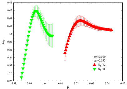
Figure 1: Susceptibility of chiral condensate $\chi_{\bar{\psi}\psi}$ as a function of coupling $\beta$ at $am=0.020$, $a\mu_{I}=0.240$ on lattice $12^{3}\times 4$ and $16^{3}\times 4$.

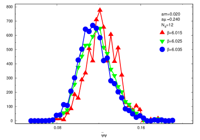
Figure 2: Reweighted distribution of $\bar{\psi}\psi$ at different $\beta$ at $am=0.020$, $a\mu_{I}=0.240$ on lattice $N_{s}=12$. $\beta=6.025$ corresponds to the pseudocritical temperature. The horizontal axis represents the value of $\bar{\psi}\psi$, and the vertical axis stands for the number of $\bar{\psi}\psi$, which is transformed from the probability of corresponding $\bar{\psi}\psi$.

Figure 3: Reweighted distribution of $\bar{\psi}\psi$ at different $\beta$ at $am=0.020$, $a\mu_{I}=0.240$ on lattice $N_{s}=16$ . $\beta=5.998$ corresponds to the pseudocritical temperature. The horizontal axis represents the value of $\bar{\psi}\psi$, and the vertical axis stands for the number of $\bar{\psi}\psi$, which is transformed from the probability of corresponding $\bar{\psi}\psi$.

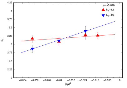
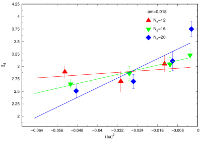
Figure 4: Binder cumulants of $\bar{\psi}\psi$ at quark masses $am=0.020$ (left panel) and $am=0.018$ (right panel) on different lattice volumes intersect at one point.

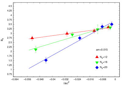
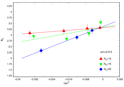
Figure 5: Binder cumulants of $\bar{\psi}\psi$ at quark masses $am=0.015$ (left panel) and $am=0.013$ (right panel) on different lattice volumes intersect at one point.

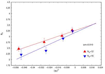
Figure 6: Binder cumulants of $\bar{\psi}\psi$ at quark mass $am=0.010$ on different lattice volumes intersect at one point.

II LATTICE FORMULATION WITH IMAGINARY CHEMICAL POTENTIAL

After introducing a pseudofermion field $\Phi$, the partition function of the system can be represented as:

$$Z = \int[dU][d\Phi^{*}][d\Phi]e^{-S_{g}-S_{f}},$$ (1)

where $S_{g}$ is the Symanzik-improved gauge action, and $S_{f}$ is the HISQ quark action with the quark chemical potential $\mu$. Here $\mu=i\mu_{I}$ is purely imaginary. For $S_{g}$, we use

$$S_{g}=\beta\left(C_{P}\sum_{x;\mu<\nu}(1-P_{\mu\nu})+C_{R}\sum_{x;\mu<\nu}(1-R_{\mu\nu})\right.$$

$$\left.+C_{T}\sum_{x;\mu<\nu<\sigma}(1-T_{\mu\nu\sigma})\right),$$ (2)

with $P_{\mu\nu},R_{\mu\nu}$, and $T_{\mu\nu\sigma}$ standing for $1/3$ of the real part of the trace of $1\times 1$, $1\times 2$ planar Wilson loops and $1\times 1\times 1$ “parallelogram” loops, respectivley,

$$P_{\mu\nu} = \frac{1}{3}{\rm Re\rm Tr}\ \raisebox{-11.38104pt}{\begin{picture}(10.0,12.0)\put(0.0,0.0){\vector(1,0){7.0}} \put(0.0,0.0){\line(1,0){10.0}} \put(10.0,0.0){\vector(0,1){7.0}} \put(10.0,0.0){\line(0,1){10.0}} \put(10.0,10.0){\vector(-1,0){7.0}} \put(10.0,10.0){\line(-1,0){10.0}} \put(0.0,10.0){\vector(0,-1){7.0}} \put(0.0,10.0){\line(0,-1){10.0}} \end{picture}}\ ,$$ (3)

$$R_{\mu\nu} = \frac{1}{3}{\rm Re\rm Tr}\ \raisebox{-11.38104pt}{\begin{picture}(20.0,12.0)\put(0.0,0.0){\vector(1,0){7.0}} \put(0.0,0.0){\line(1,0){10.0}} \put(10.0,0.0){\vector(1,0){7.0}} \put(10.0,0.0){\line(1,0){10.0}} \put(20.0,0.0){\vector(0,1){7.0}} \put(20.0,0.0){\line(0,1){10.0}} \put(20.0,10.0){\vector(-1,0){7.0}} \put(20.0,10.0){\line(-1,0){10.0}} \put(10.0,10.0){\vector(-1,0){7.0}} \put(10.0,10.0){\line(-1,0){10.0}} \put(0.0,10.0){\vector(0,-1){7.0}} \put(0.0,10.0){\line(0,-1){10.0}} \put(10.0,1.0){\circle*{0.1}}\put(10.0,2.0){\circle*{0.1}}\put(10.0,3.0){\circle*{0.1}}\put(10.0,4.0){\circle*{0.1}}\put(10.0,5.0){\circle*{0.1}}\put(10.0,6.0){\circle*{0.1}}\put(10.0,7.0){\circle*{0.1}}\put(10.0,8.0){\circle*{0.1}}\put(10.0,9.0){\circle*{0.1}} \end{picture}}\ ,$$ (4)

$$T_{\mu\nu\sigma} = \frac{1}{3}{\rm Re\rm Tr}\ \raisebox{-11.38104pt}{\begin{picture}(16.0,16.0)\put(0.0,0.0){\vector(1,0){7.0}} \put(0.0,0.0){\line(1,0){10.0}} \put(10.0,0.0){\vector(2,1){4.0}} \put(10.0,0.0){\line(2,1){6.0}} \put(16.0,3.0){\vector(0,1){7.0}} \put(16.0,3.0){\line(0,1){10.0}} \put(16.0,13.0){\vector(-1,0){7.0}} \put(16.0,13.0){\line(-1,0){10.0}} \put(6.0,13.0){\vector(-2,-1){4.0}} \put(6.0,13.0){\line(-2,-1){6.0}} \put(0.0,10.0){\vector(0,-1){7.0}} \put(0.0,10.0){\line(0,-1){10.0}} \put(1.0,0.5){\circle*{0.1}}\put(2.0,1.0){\circle*{0.1}}\put(3.0,1.5){\circle*{0.1}}\put(4.0,2.0){\circle*{0.1}}\put(5.0,2.5){\circle*{0.1}}\put(6.0,3.0){\circle*{0.1}} \put(6.0,4.0){\circle*{0.1}}\put(6.0,5.0){\circle*{0.1}}\put(6.0,6.0){\circle*{0.1}}\put(6.0,7.0){\circle*{0.1}}\put(6.0,8.0){\circle*{0.1}}\put(6.0,9.0){\circle*{0.1}}\put(6.0,10.0){\circle*{0.1}}\put(6.0,11.0){\circle*{0.1}}\put(6.0,12.0){\circle*{0.1}} \put(7.0,3.0){\circle*{0.1}}\put(8.0,3.0){\circle*{0.1}}\put(9.0,3.0){\circle*{0.1}}\put(10.0,3.0){\circle*{0.1}}\put(11.0,3.0){\circle*{0.1}}\put(12.0,3.0){\circle*{0.1}}\put(13.0,3.0){\circle*{0.1}}\put(14.0,3.0){\circle*{0.1}}\put(15.0,3.0){\circle*{0.1}} \end{picture}}\ ,$$ (5)

The coefficents $C_{P},C_{R}$, and $C_{T}$ are tadpole improved Bazavov:2010ru ,

$$C_{P} = 1.0,$$ (6)

$$C_{R} = \frac{-1}{20u_{0}^{2}}\left(1-\left(0.6264-1.1746n_{f}\right){\rm ln}(u_{0})\right),$$ (7)

$$C_{T} = \frac{1}{u_{0}^{2}}\left(0.0433-0.0156n_{f}\right){\rm ln}(u_{0}).$$ (8)

with $u_{0}=(<P_{\mu\nu}>)^{3/4}$.

The HISQ action with pseudofermion field $\Phi$ is

$$S_{f}=\left<\Phi\left|\left[M^{{\dagger}}[U]M[U]\right]^{-n_{f}/4}\right|\Phi\right>,$$ (9)

where the form of $M_{x,y}\left[U\right]=2m_{x,y}+2\lower-0.77496pt\hbox{\makebox[-1.0pt][l]{\,/}}D_{x,y}(U)$ with $2\lower-0.77496pt\hbox{\makebox[-1.0pt][l]{\,/}}D_{x,y}(U)$ reading

$$2\lower-0.77496pt\hbox{\makebox[-1.0pt][l]{\,/}}D_{x,y}=\sum\limits_{\rho=1}^{3}\left\{X_{\rho}(x)\delta_{x+\hat{\rho},y}-X_{\rho}^{\dagger}(x-\hat{\rho})\delta_{x-\hat{\rho},y}\right\}$$

$$+\sum\limits_{\rho=1}^{3}\left\{N_{\rho}(x)\delta_{x+3\hat{\rho},y}\right.-\left.N_{\rho}^{\dagger}(x-3\hat{\rho})\delta_{x-3\hat{\rho},y}\right\}$$

$$+\left\{e^{ia\mu_{I}}X_{4}(x)\delta_{x+\hat{4},y}-e^{-ia\mu_{I}}X_{4}^{\dagger}(x-\hat{4})\delta_{x-\hat{4},y}\right\}+$$

$$\left\{e^{i3a\mu_{I}}N_{4}(x)\delta_{x+3\hat{4},y}-e^{-i3a\mu_{I}}N_{4}^{\dagger}(x-3\hat{4})\delta_{x-3\hat{4},y}\right\}.$$ (10)

The Dirac operator $\lower-0.77496pt\hbox{\makebox[-1.0pt][l]{\,/}}D$ is constructed from smeared links Bazavov:2010ru . The fundamental gauge links are $U_{\mu}(x)$, the fat links after a level-1 fat7 smearing are $V_{\mu}(x)$, the reunitarized links are $W_{\mu}(x)$, and the fat links after level-2 asqtad smearing are $X_{\mu}(x)$. For simplicity, we use $N_{x,\rho}=W_{\rho}(x)W_{\rho}(x+\hat{\rho})W_{\rho}(x+2\hat{\rho})$. The staggered fermion phases are absorbed into the link variables. $\hat{\rho}$ and $\hat{4}$ are the unit vectors along $\rho-$direction and $4$ direction, respectively.

In the study to address the chiral transition, it is natural to choose the chiral condensate as our observable. The chiral condensate is defined as:

$$X=\bar{\psi}\psi=\frac{1}{N_{s}^{3}N_{t}}{\rm Tr}(M^{-1}),$$ (11)

$N_{s}$ and $N_{t}$ are the spatial and temporal extent of lattice, respectively. To simplify notation, we use $X$ to represent the chiral condensate. The susceptibility of chiral condensate is defined as

$$\chi_{\bar{\psi}\psi}=\left\langle(X-\langle X\rangle)^{2}\right\rangle.$$ (12)

We also calculate the Binder cumulant of chiral condensate which is defined as:

$$B_{4}=\left\langle(X-\langle X\rangle)^{4}\right\rangle/\left\langle(X-\langle X\rangle)^{2}\right\rangle^{2}.$$ (13)

The Binder cumulant of the chiral condensate can be expanded around $a\mu_{c}$ as  Bonati:2014kpa ; Philipsen:2016hkv

$$B_{4}(am,a\mu)=B_{4}(am,a\mu_{c})+b_{1}((a\mu)^{2}-(a\mu_{c})^{2})N_{s}^{1/\nu}+\cdots.$$ (14)

III MC SIMULATION RESULTS

Before presenting the simulation results, we describe the computation details. Simulations are carried out at quark masses $am=0.020,\,$ $0.018,\,$ $0.015,\,$ $0.013,\,$ $0.010$. The Rational Monte Carlo algorithm Clark:2003na ; Clark:2006wp ; Clark:2006fx is used to generate configurations. We use different molecular dynamics step sizes for the gauge and fermion parts of the action, with three gauge steps for each fermion step SEXTON . The Omelyan integration algorithm Takaishi:2005tz ; omeylan is employed for the gauge and fermion action. For the molecular dynamics evolution, we use a ninth rational function to approximate $[M^{+}(U)M(U)]^{-n_{f}/4}$ for the pseudofermion field. For the heat bath updating and for computing the action at the beginning and end of the molecular dynamics trajectory, two tenth rational function are used to approximate $[M^{+}(U)M(U)]^{n_{f}/8}$ and $[M^{+}(U)M(U)]^{-n_{f}/8}$, respectively. The step is chosen to ensure the acceptance rate is around $72\%\!\!-\!\!82\%$. Five thousand trajectories of configuration are taken as warmup from a cold start. To fill in observables at additional $\beta$ values, we employ the Ferrenberg-Swendsen reweighting method Ferrenberg:1989ui .

At a certain pair of the value of quark mass $am$ and chemical potential $a\mu_{I}$, we scan the $\beta$ values and calculate the susceptibility $\chi_{\bar{\psi}\psi}$ of chiral condensate $\bar{\psi}\psi$. The location of peak of susceptibility of the chiral condensate is interpreted as the transition point. For clarity, we only present the results of $\chi_{\bar{\psi}\psi}$ on lattice $N_{s}=12$ and $N_{s}=16$ at $am=0.020$, $a\mu_{I}=0.240$ in Fig 1. Similar behavior of $\chi_{\bar{\psi}\psi}$ can be observed at other couples of $(am,a\mu_{I})$ on different lattice volumes.

To monitor the change of $\bar{\psi}\psi$ near the pseudotransition point, we present the reweighted distribution of $\bar{\psi}\psi$ at three temperatures around the transition on $N_{s}=12$ and $N_{s}=16$ at $am=0.020$ , $a\mu_{I}=0.240$ in Figs. 2 and 3, respectively. The horizontal axis represents the value of $\bar{\psi}\psi$, and the vertical axis stands for the number of $\bar{\psi}\psi$ which is transformed from the probability of corresponding $\bar{\psi}\psi$. From Figs. 2 and 3, we can find that the reweighted distribution of $\bar{\psi}\psi$ does not show the signal of first-order transition. At other quark masses, similar behavior can be observed.

The results of critical couplings $\beta_{c}$ and the corresponding $B_{4}$ values on different spatial volumes at different quark masses $am$ are summarized in Table. 1. These $\beta_{c}$’s are determined from the locations of peak susceptibility $\chi_{\bar{\psi}\psi}$ of chiral condensate $\bar{\psi}\psi$.

Table 1: Results of critical couplings $\beta_{c}$ obtained by the locations of peak of $\chi_{\bar{\psi}\psi}$ and the $B_{4}$ values on different spatial volumes at different quark masses $am$.

	$N_{s}=8$			$N_{s}=12$			$N_{s}=16$			$N_{s}=20$
$am$	$a\mu_{I}$	$\beta_{c}$	$B_{4}$	$a\mu_{I}$	$\beta_{c}$	$B_{4}$	$a\mu_{I}$	$\beta_{c}$	$B_{4}$	$a\mu_{I}$	$\beta_{c}$	$B_{4}$
0.010	0.040	5.998(40)	3.68(12)	0.050	6.058(20)	3.28(13)	0.045	6.018(20)	3.25(10)	-	-	-
	0.100	6.018(40)	5.33(12)	0.110	6.048(20)	3.04(12)	0.105	5.998(20)	2.93(12)	-	-	-
	0.160	6.008(20)	4.03(13)	0.170	5.988(60)	2.77(17)	0.165	5.998(40)	2.39(14)	-	-	-
	0.220	5.988(20)	4.31(10)	0.230	6.048(20)	2.48(11)	0.225	6.098(20)	2.22(22)	-	-	-
0.013	0.040	5.998(40)	3.39(15)	0.035	6.008(60)	3.31(10)	0.030	6.008(60)	3.55(11)	-	-	-
	0.090	5.998(20)	3.42(11)	0.085	5.968(40)	3.28(18)	0.080	6.008(10)	3.08(14)	0.070	6.048(10)	3.21(13)
	0.140	5.988(30)	3.43(11)	0.135	5.988(28)	3.17(12)	0.130	5.964(30)	2.23(11)	0.110	6.048(30)	2.91(11)
	0.190	6.048(24)	3.94(12)	0.185	5.984(34)	3.09(11)	0.180	6.090(30)	1.84(11)	0.170	6.098(50)	2.34(10)
0.015	0.050	6.078(30)	2.35(22)	0.065	6.018(20)	3.35(14)	0.055	5.988(30)	3.33(13)	0.045	6.028(20)	3.51(14)
	0.100	5.968(40)	3.78(11)	0.115	6.008(70)	3.14(12)	0.105	5.988(20)	3.22(25)	0.090	6.028(20)	3.37(15)
	0.160	6.028(30)	3.90(11)	0.175	6.068(110)	2.98(14)	0.165	6.058(30)	2.93(14)	0.150	6.098(10)	2.74(14)
	0.220	5.988(10)	4.10(13)	0.230	6.028(20)	2.74(12)	0.225	5.968(100)	2.12(18)	0.210	5.968(10)	1.52(16)
0.018	0.060	5.978(30)	2.20(12)	0.065	6.018(20)	3.05(10)	0.055	6.018(40)	3.24(12)	0.050	6.058(10)	3.75(15)
	0.110	5.958(50)	2.69(23)	0.115	5.978(50)	3.05(16)	0.105	6.018(10)	3.04(14)	0.100	5.978(40)	3.12(19)
	0.170	5.968(90)	3.22(12)	0.175	5.968(40)	2.70(21)	0.165	5.998(30)	2.86(14)	0.160	5.978(10)	2.70(14)
	0.230	5.988(30)	3.61(14)	0.235	6.028(20)	2.89(12)	0.225	6.018(20)	2.65(10)	0.220	5.988(40)	2.51(14)
0.020	0.060	5.998(20)	2.16(11)	0.120	6.005(30)	3.26(10)	0.120	6.038(80)	3.10(16)	-	-	-
	0.130	5.998(90)	3.19(17)	0.150	6.078(70)	3.28(13)	0.150	6.018(40)	3.40(14)	-	-	-
	0.190	6.048(40)	3.31(14)	0.200	6.058(30)	3.08(10)	0.200	6.078(40)	3.12(10)	-	-	-
	0.250	5.998(20)	3.62(10)	0.240	6.025(10)	3.18(10)	0.240	5.998(50)	2.87(11)	-	-	-

Table 2: Results of critical chemical potential $a\mu_{c}$ at  different quark masses obtained by fitting $B_{4}=1.604+b\left((a\mu)^{2}-(a\mu_{c})^{2}\right)$ to data on lattice $N_{s}=20$.

$am$	$b$	$a\mu_{c}$	$r$-square
0.013	35.84(7)	0.2218(2)	0.998
0.015	48.23(12))	0.209(1)	0.993
0.018	24.28(27)	0.282(1)	0.899

After the critical couplings $\beta_{c}$ and the corresponding $B_{4}$ values are obtained, we can monitor their behavior on different lattice spatial volumes at a certain quark mass. The results are presented in Figs. 4,5,and 6. From Figs. 4,5, and 6, we can find that with the decreasing absolute value of the chemical potential, the $B_{4}$ value increases on lattice $N_{s}=12,\,16\,$ and $N_{s}=20$. On the contrary, on lattice $N_{s}=8$, the values of $B_{4}$ fall with the declining absolute value of chemical potential due to large finite size effect. So we do not include them in Figs. 4,5, and 6. Nevertheless, at a certain quark mass, we can find that the $B_{4}$ values on different lattice volume intersect approximately at one point.

However, from Figs. 4,5, and 6, we can find that the values of $B_{4}$ on different lattice sizes approximately intersect at $B_{4}(am,a\mu_{c})\sim 3$. We think that it is because of large finite lattice effects. To gain some understanding about the result, we fit expression

$$B_{4}=1.604+b\left((a\mu)^{2}-(a\mu_{c})^{2}\right)$$ (15)

to the data on the $N_{s}=20$ lattice to get the critical $a\mu_{c}$. The results are presented in Table 2.

From the results in Table 2, we can see that the critical $a\mu_{c}$’s on lattice $20^{3}\times 4$ are approximately in a reasonable region, which should be smaller than 0.262 on the $N_{t}=4$ lattice. If we use Eq. (15) to fit the data on the smaller lattice, it can be found that the critical $a\mu_{c}$’s are much larger than 0.262. Moreover, the $r$-square values in Table 2 that are close to 1 show that the fit is good. All these facts imply that the smaller lattices have significant finite volume effects.

From Fig. 8 in Ref. Bonati:2014kpa , we can see that the value of $B_{4}$ at the intersection point is 1.604, which is consistent with the $Z(2)$ universality class value. This shows that the finite lattice volume effects in Ref. Bonati:2014kpa are very small.

IV DISCUSSIONS

We have made a simulation in an attempt to understand the nature of the phase transition of QCD with two massless flavors with the one quark-loop Symanzik-improved gauge action and the HISQ fermion action by using the method proposed in Ref. Bonati:2014kpa at the quark masses $am=0.020,\,0.018,\,0.015,\,0.013,\,0.010$.

In our simulation, we found that the Binder cumulants of the chiral condensate on different lattice volumes at one quark mass intersect at one point. The value of $B_{4}$ at the intersection point $B_{4}(am,a\mu_{c})$ was renormalization-invariant. At the quark masses we used , the value of $B_{4}$ at the intersection point $B_{4}(am,a\mu_{c})$ was around $3$.

At a nonvanishing quark mass, an additive and multiplicative renormalization of $\bar{\psi}\psi$ was needed to define the order parameter $\bar{\psi}\psi$ when the scaling property was under consideration Ejiri:2009ac ; Bazavov:2011nk ; Cheng:2007jq . Equations. (9) and (12) in Ref. Ejiri:2009ac , Eq. (36) in Ref. Cheng:2007jq , and Eq. (30) in Ref. Bazavov:2011nk were used to subtract the finite quark mass influence on $\bar{\psi}\psi$. However, if we start from Eqs. (12) and (13) and subtract the finite quark mass influence from the chiral condensate, then put the subtracted chiral condensate into Eqs. (12) and (13), we think that multiplicative or additive renormalization of $\bar{\psi}\psi$ would have no effect on the value of $B_{4}(am,a\mu_{c})$.

If we can detect the $Z(2)$ transition line, the value of $B_{4}$ at the intersection point should be $1.604$ Bonati:2014kpa ; Philipsen:2016hkv . However, in our simulation, $B_{4}(am,a\mu_{c})\sim 3$ deviated from the $Z(2)$ universality class value. If we just used Eq. (15) to fit the data on $N_{s}=20$ lattice, we found the fit was good and the $a\mu_{c}$’s obtained were reasonable. So, we think that $B_{4}(am,a\mu_{c})\sim 3$ is because of large finite volume effects as described in Sec. III.

Similar behavior was observed in Ref. Jin:2017jjp , in which Wilson-type fermions were employed to determine the critical point separating the crossover from the first-order phase transition region for three-flavour QCD. In that research, the value of kurtosis of the chiral condensate at the intersection point deviated from the universality class value on the $N_{t}=8,\,10$ lattice due to finite volume correction. This observation indicates that simulation with HISQ action along this direction on the $N_{s}>20$ lattice is of great importance.

- (1) K. Fukushima and T. Hatsuda, Rept. Prog. Phys. 74 014001 (2011).
- (2) K. Fukushima, J. Phys. G 39 013101 (2012).
- (3) G. Aarts, J. Phys. Conf. Ser. 706, no. 2, 022004 (2016) doi:10.1088/1742-6596/706/2/022004 [arXiv:1512.05145 [hep-lat]].
- (4) R. D. Pisarski and F. Wilczek, Phys. Rev. D 29, 338 (1984). doi:10.1103/PhysRevD.29.338
- (5) A. Butti, A. Pelissetto and E. Vicari, JHEP 0308, 029 (2003) doi:10.1088/1126-6708/2003/08/029 [hep-ph/0307036].
- (6) A. Pelissetto and E. Vicari, Phys. Rev. D 88, no. 10, 105018 (2013) doi:10.1103/PhysRevD.88.105018 [arXiv:1309.5446 [hep-lat]].
- (7) T. Sato and N. Yamada, Phys. Rev. D 91, no. 3, 034025 (2015) doi:10.1103/PhysRevD.91.034025 [arXiv:1412.8026 [hep-lat]].
- (8) S. Ejiri et al., Phys. Rev. D 80, 094505 (2009) doi:10.1103/PhysRevD.80.094505 [arXiv:0909.5122 [hep-lat]].
- (9) F. Karsch and E. Laermann, Phys. Rev. D 50, 6954 (1994) doi:10.1103/PhysRevD.50.6954 [hep-lat/9406008].
- (10) A. Ali Khan et al. [CP-PACS Collaboration], Phys. Rev. D 63, 034502 (2001) doi:10.1103/PhysRevD.63.034502 [hep-lat/0008011].
- (11) S. Ejiri, R. Iwami and N. Yamada, Phys. Rev. D 93, no. 5, 054506 (2016) doi:10.1103/PhysRevD.93.054506 [arXiv:1511.06126 [hep-lat]].
- (12) F. Burger et al. [tmfT Collaboration], Phys. Rev. D 87, no. 7, 074508 (2013) doi:10.1103/PhysRevD.87.074508 [arXiv:1102.4530 [hep-lat]].
- (13) S. Aoki et al. [JLQCD Collaboration], Phys. Rev. D 57, 3910 (1998) doi:10.1103/PhysRevD.57.3910 [hep-lat/9710048].
- (14) C. W. Bernard et al., Phys. Rev. Lett. 78, 598 (1997) doi:10.1103/PhysRevLett.78.598 [hep-lat/9611031].
- (15) Y. Iwasaki, K. Kanaya, S. Kaya and T. Yoshie, Phys. Rev. Lett. 78, 179 (1997) doi:10.1103/PhysRevLett.78.179 [hep-lat/9609022].
- (16) C. Bonati, P. de Forcrand, M. D’Elia, O. Philipsen and F. Sanfilippo, Phys. Rev. D 90, no. 7, 074030 (2014) doi:10.1103/PhysRevD.90.074030 [arXiv:1408.5086 [hep-lat]].
- (17) O. Philipsen and C. Pinke, Phys. Rev. D 93, no. 11, 114507 (2016) doi:10.1103/PhysRevD.93.114507 [arXiv:1602.06129 [hep-lat]].
- (18) F. Cuteri, O. Philipsen and A. Sciarra, arXiv:1711.05658 [hep-lat].
- (19) M. D’Elia, A. Di Giacomo and C. Pica, Phys. Rev. D 72, 114510 (2005) doi:10.1103/PhysRevD.72.114510 [hep-lat/0503030].
- (20) G. Cossu, S. Aoki, H. Fukaya, S. Hashimoto, T. Kaneko, H. Matsufuru and J. I. Noaki, Phys. Rev. D 87, no. 11, 114514 (2013) Erratum: [Phys. Rev. D 88, no. 1, 019901 (2013)] doi:10.1103/PhysRevD.88.019901, 10.1103/PhysRevD.87.114514 [arXiv:1304.6145 [hep-lat]].
- (21) S. Aoki, H. Fukaya and Y. Taniguchi, Phys. Rev. D 86, 114512 (2012) doi:10.1103/PhysRevD.86.114512 [arXiv:1209.2061 [hep-lat]].
- (22) M. Fukugita, H. Mino, M. Okawa and A. Ukawa, Phys. Rev. D 42, 2936 (1990). doi:10.1103/PhysRevD.42.2936
- (23) C. W. Bernard, C. E. Detar, S. A. Gottlieb, U. M. Heller, J. Hetrick, K. Rummukainen, R. L. Sugar and D. Toussaint, Phys. Rev. D 61, 054503 (2000) doi:10.1103/PhysRevD.61.054503 [hep-lat/9908008].
- (24) H. B. Meyer, PoS LATTICE 2015, 014 (2016) [arXiv:1512.06634 [hep-lat]].
- (25) H. Ohno, U. M. Heller, F. Karsch and S. Mukherjee, PoS LATTICE 2012, 095 (2012) [arXiv:1211.2591 [hep-lat]].
- (26) V. Dick, F. Karsch, E. Laermann, S. Mukherjee and S. Sharma, Phys. Rev. D 91, no. 9, 094504 (2015) doi:10.1103/PhysRevD.91.094504 [arXiv:1502.06190 [hep-lat]].
- (27) B. B. Brandt, A. Francis, H. B. Meyer, O. Philipsen, D. Robaina and H. Wittig, JHEP 1612, 158 (2016) doi:10.1007/JHEP12(2016)158 [arXiv:1608.06882 [hep-lat]].
- (28) A. Tomiya, G. Cossu, S. Aoki, H. Fukaya, S. Hashimoto, T. Kaneko and J. Noaki, Phys. Rev. D 96, no. 3, 034509 (2017) Addendum: [Phys. Rev. D 96, no. 7, 079902 (2017)] doi:10.1103/PhysRevD.96.034509, 10.1103/PhysRevD.96.079902 [arXiv:1612.01908 [hep-lat]].
- (29) A. Bazavov et al. [HotQCD Collaboration], Phys. Rev. D 86, 094503 (2012) doi:10.1103/PhysRevD.86.094503 [arXiv:1205.3535 [hep-lat]].
- (30) C. Bonati, P. de Forcrand, M. D’Elia, O. Philipsen and F. Sanfilippo, PoS LATTICE 2011, 189 (2011) [arXiv:1201.2769 [hep-lat]].
- (31) A. Bazavov et al., Phys. Rev. D 85, 054503 (2012) doi:10.1103/PhysRevD.85.054503 [arXiv:1111.1710 [hep-lat]].
- (32) A. Bazavov et al. [MILC Collaboration], Rev. Mod. Phys. 82 1349 (2010).
- (33) Z. Hao, G. M. von Hippel, R. R. Horgan, Q. J. Mason and H. D. Trottier, Phys. Rev. D 76, 034507 (2007) doi:10.1103/PhysRevD.76.034507 [arXiv:0705.4660 [hep-lat]].
- (34) K. Symanzik, Nucl. Phys. B 226, 187 (1983). doi:10.1016/0550-3213(83)90468-6
- (35) M. Luscher and P. Weisz, Phys. Lett. 158B, 250 (1985). doi:10.1016/0370-2693(85)90966-9
- (36) G. P. Lepage and P. B. Mackenzie, Phys. Rev. D 48, 2250 (1993) doi:10.1103/PhysRevD.48.2250 [hep-lat/9209022].
- (37) M. G. Alford, W. Dimm, G. P. Lepage, G. Hockney and P. B. Mackenzie, Phys. Lett. B 361, 87 (1995) doi:10.1016/0370-2693(95)01131-9 [hep-lat/9507010].
- (38) A. Hart et al. [HPQCD Collaboration], Phys. Rev. D 79, 074008 (2009) doi:10.1103/PhysRevD.79.074008 [arXiv:0812.0503 [hep-lat]].
- (39) E. Follana et al. [HPQCD and UKQCD Collaborations], Phys. Rev. D 75, 054502 (2007) doi:10.1103/PhysRevD.75.054502 [hep-lat/0610092].
- (40) S. Naik, 1989 Nucl. Phys. B 316 238 (1989).
- (41) C. W. Bernard et al. [MILC Collaboration], Phys. Rev. D 58 014503 (1998).
- (42) P. Cea, L. Cosmai and A. Papa, Phys. Rev. D 89, no. 7, 074512 (2014) doi:10.1103/PhysRevD.89.074512 [arXiv:1403.0821 [hep-lat]].
- (43) A. Bazavov et al. [MILC Collaboration], Phys. Rev. D 82, 074501 (2010) doi:10.1103/PhysRevD.82.074501 [arXiv:1004.0342 [hep-lat]].
- (44) M. A. Clark and A. D. Kennedy, Nucl. Phys. Proc. Suppl. 129 850 (2004).
- (45) M. A. Clark and A. D. Kennedy, Phys. Rev. D 75 011502 (2007).
- (46) M. A. Clark and A. D. Kennedy, Phys. Rev. Lett. 98 051601 (2007).
- (47) J.C. Sexton and D.H. Weingarten, Nucl. Phys. B380, 665 (1992).
- (48) T. Takaishi and P. De Forcrand, Phys. Rev. E 73 036706 (2006).
- (49) I. P. Omeylan, I. M. Mryglod and R. Folk, Comp. Phys. Comm. 151 272 (2003).
- (50) A. M. Ferrenberg and R. H. Swendsen, Phys. Rev. Lett. 63, 1195 (1989).
- (51) M. Cheng et al., Phys. Rev. D 77, 014511 (2008) doi:10.1103/PhysRevD.77.014511 [arXiv:0710.0354 [hep-lat]].
- (52) X. Y. Jin, Y. Kuramashi, Y. Nakamura, S. Takeda and A. Ukawa, Phys. Rev. D 96, no. 3, 034523 (2017) doi:10.1103/PhysRevD.96.034523 [arXiv:1706.01178 [hep-lat]].
- (53) http://physics.utah.edu/~detar/milc/.
- (54) http://crd-legacy.lbl.gov/~dhbailey/mpdist/.