Singularities in Einstein-conformally coupled Higgs cosmological models

Abstract

The dynamics of Einstein–conformally coupled Higgs field (EccH) system is investigated near the initial singularities in the presence of Friedman–Robertson–Walker symmetries. We solve the field equations asymptotically up to fourth order near the singularities analytically, and determine the solutions numerically as well. We found all the asymptotic, power series singular solutions, which are (1) solutions with a scalar polynomial curvature singularity but the Higgs field is bounded (‘Small Bang’), or (2) solutions with a Milne type singularity with bounded spacetime curvature and Higgs field, or (3) solutions with a scalar polynomial curvature singularity and diverging Higgs field (‘Big Bang’). Thus, in the present EccH model there is a new kind of physical spacetime singularity (‘Small Bang’). We also show that, in a neighbourhood of the singularity in these solutions, the Higgs sector does not have any symmetry breaking instantaneous vacuum state, and hence then the Brout–Englert–Higgs mechanism does not work. The large scale behaviour of the solutions is investigated numerically as well. In particular, the numerical calculations indicate that there are singular solutions that cannot be approximated by power series.

1 Introduction

The two most successful theories of the 20th century physics are General Relativity (see e.g. [1]) and the Standard Model of particle physics (see e.g. [2]). In our previous paper [3] we investigated the origin of the rest masses of the classical fields of the Einstein–Standard Model system in which the Higgs field is conformally coupled to gravity (‘Einstein–conformally coupled–Standard Model’, or shortly, EccSM system). In this theory, in addition to the familiar Big Bang singularity, another (slightly less violent) singularity may also emerge (‘Small Bang’). In the latter all the matter field variables are finite, and this singularity corresponds to a special, finite value of the pointwise norm of the Higgs field. In [3] we primarily concentrated on how the Brout–Englert–Higgs (or shortly BEH) mechanism works in this system. We found that there could be extreme gravitational situations in which the system does not have any vacuum state, even instantaneous ones, and hence the notion of rest mass of the Higgs field cannot be introduced at all and the gauge and the fermion fields are still massless. When the system has vacuum states, then these states are only instantaneous and necessarily gauge symmetry breaking. Then, via the BEH mechanism, the fields get rest mass. Therefore, the rest mass (and electric charge in the Weinberg–Salam model) has a non-trivial genesis after the initial singularity.

To derive these results it was enough to consider only the kinematical structure of the EccSM system (using only the constraint equations) [3], but we did not investigate its dynamics (i.e. we did not use the evolution equations). In the present paper our aim is two-fold: (1) to clarify the dynamics of the model near both the points where the Higgs field takes the critical value above (where the Small Bang is expected to be present) and the Big Bang singularity, and, in particular, to demonstrate that the Small Bang is not fictitious, but it is a genuine scalar polynomial curvature singularity; and (2) to justify the key observation of [3] that the rest masses of the classical fields could emerge in a non-trivial ‘phase transition’ in the very early period of the history of the Universe in a dynamical process after the initial singularity. In this very early era the dominant matter field is the Higgs field. Thus, for the sake of simplicity, we consider only the Einstein–conformally coupled Higgs (or shortly EccH) system in which the Higgs field is a single real self-interacting scalar field $\Phi$ in the presence of Friedman–Robertson–Walker (or FRW) symmetries. We determine all the asymptotic (power series) solutions near the singularities. Since the asymptotic, power series techniques are appropriate to determine the behaviour of the solutions only in the very small neighbourhoods of the singularities, to see the structure of the solutions on larger scales, we should find numerical solutions as well.

We found all the asymptotic singular (power series) solutions of the field equations, which are (1) solutions with a scalar polynomial curvature singularity but in which the Higgs field is bounded (‘Small Bang’), or (2) solutions with a Milne type singularity [4] with bounded spacetime curvature and Higgs field, or (3) solutions with a scalar polynomial curvature singularity and diverging Higgs field (‘Big Bang’). The solutions with a Small Bang or a Big Bang singularity form a 1-parameter family of solutions for any value $k=\pm 1$ of the discrete cosmological parameter. The solutions for $k=0$ are determined (up to an overall scale factor) by the parameters of the theory. The solutions with a Milne type singularity exist only for $k=-1$, but these depend on a continuous parameter. The latter solutions can be continued through the (fictitious) Milne type singularity, describing a contracting and then expanding universe. Already these asymptotic solutions answer the questions above: (1) the Small Bang singularity is a genuine physical spacetime singularity, and (2) in a neighbourhood of the initial singularity there is, indeed, a very early period in the history of the Universe when the BEH mechanism does not work and hence the fields of the Standard Model could not get non-zero rest mass via the BEH mechanism.

We solve the equations of motion numerically, too. We show that the approximate, power series solutions can be extended from $10^{-3}$ to $10^{22}$ Planck times, and this time interval has an overlap with the era governed by the weak interactions. Moreover, we found that, in addition to the power series type singular solutions, there are other singular solutions that cannot be approximated by any power series in a neighbourhood of the singularity.

In section 2 we recall briefly the key points of the EccH model with the FRW symmetries. Section 3 is devoted to the asymptotic (power series) solutions in which the Higgs field remain bounded; while the solutions with diverging Higgs field are determined in section 4. The numerical results are presented and discussed in section 5; and the results and the main messages of the paper are summarized in section 6.

Our conventions are those of [3]. In particular, the signature of the spacetime metric is $(+,-,-,-)$ and Einstein’s equations take the form $R_{ab}-\frac{1}{2}Rg_{ab}=-\kappa T_{ab}-\Lambda g_{ab}$. Here $\Lambda$ is the cosmological constant and $\kappa:=8\pi G$ with Newton’s gravitational constant $G$.

2 The EccSM system with FRW symmetries

2.1 The field equations

Let $\Sigma_{t}:=\{t={\rm const}\}$ be the foliation of the FRW symmetric spacetime by the transitivity surfaces of the isometries, where $t$ is the proper time coordinate along the integral curves of the future pointing unit normals of the hypersurfaces $\Sigma_{t}$ (see e.g. [1]). Thus the lapse is $N=1$. Let $S=S(t)$ be the (strictly positive) scale function for which the induced metric on $\Sigma_{t}$ is $h_{ab}=S^{2}{}_{1}h_{ab}$, where ${}_{1}h_{ab}$ is the standard negative definite metric on the unit 3-sphere, the flat 3-space and the unit hyperboloidal 3-space, respectively, for $k=1,0,-1$. The extrinsic curvature of the hypersurfaces is $\chi_{ab}=(\dot{S}/S)h_{ab}$, where over-dot denotes derivative with respect to $t$, and hence its trace is $\chi=3\dot{S}/S$. The curvature scalar of the intrinsic Levi-Civita connection is ${\cal R}=6k/S^{2}$. In the initial value formulation of Einstein’s theory the initial data are $h_{ab}$ and $\chi_{ab}$, and hence in the present case $S$ and $\dot{S}$, restricted by the constraint equations.

For the metric with FRW symmetries Einstein’s equations are well known [1] to reduce to

$$3\bigl{(}\frac{\dot{S}}{S}\bigr{)}^{2}=\Lambda+\kappa\varepsilon-3\frac{k}{S^{2}},\hskip 20.0pt3\frac{\ddot{S}}{S}=\Lambda-\frac{1}{2}\kappa\bigl{(}\varepsilon+3P\bigr{)},$$ (2.1)

where $\varepsilon$ is the energy density and $P$ is the isotropic pressure in the energy-momentum tensor of the matter fields. The first of these equations is the Hamiltonian constraint, while the second is the evolution equation. (The momentum constraint is satisfied identically.)

If the fields of the matter sector of the EccSM system are required to be invariant under the isometries of the spacetime, then all the fields with spatial vector or spinor index must be vanishing and the Higgs field $\Phi^{\bf i}$ and its canonical momentum, $\Pi^{\bf i}=\dot{\Phi}^{\bf i}+\frac{1}{3}\chi\Phi^{\bf i}$, must be constant on the hypersurfaces $\Sigma_{t}$. Thus, the EccSM system restricted by the FRW symmetries reduces to the Einstein–conformally coupled Higgs (EccH) system. For the sake of simplicity, instead of a non-trivial multiplet of scalar fields, we consider the Higgs field only to be a single real scalar field $\Phi$, the gauge group to be $\mathbb{Z}_{2}$ acting on the Higgs field as $\Phi\mapsto-\Phi$, and the Lagrangian for the Higgs field is

$${\cal L}_{H}:=\frac{1}{2}g^{ab}(\nabla_{a}\Phi)(\nabla_{b}\Phi)-\frac{1}{12}R\Phi^{2}-\frac{1}{2}\mu^{2}\Phi^{2}-\frac{1}{4}\lambda\Phi^{4}.$$

Here $R$ is the curvature scalar of the spacetime, $\lambda>0$ is the Higgs self-interaction and $\mu^{2}<0$ is the mass parameter. (In the $\hbar=c=1$ units the numerical value of the various constants of the model are $\Lambda=10^{-58}cm^{-2}$, $6/\kappa=8.6\times 10^{64}cm^{-2}$, $\lambda=1/8$ and $\mu^{2}=-1.8\times 10^{31}cm^{-2}$.) A simple calculation gives that the trace of the energy-momentum tensor of the Higgs field is $\mu^{2}\Phi^{2}$. Then, using the trace of Einstein’s equation, $R=4\Lambda+\kappa\mu^{2}\Phi^{2}$, the field equation for the Higgs field takes the form

$$\ddot{\Phi}+3\frac{\dot{S}}{S}\dot{\Phi}=-\bigl{(}\mu^{2}+\frac{2}{3}\Lambda\bigr{)}\Phi-\bigl{(}\lambda+\frac{1}{6}\kappa\mu^{2}\bigr{)}\Phi^{3}.$$ (2.2)

The initial data for the evolution equations is the quadruplet $(\Phi,S;\dot{\Phi},\dot{S})$, or, equivalently, $(\Phi,S;\Pi,\chi)$, subject to the constraint part of (2.1). Thus the configuration space ${\cal Q}$ of the dynamical system (2.1)-(2.2) is the set of the pairs $(\Phi,S)$, where $S>0$; while its velocity and momentum phase spaces, $T{\cal Q}$ and $T^{*}{\cal Q}$, are the sets of the quadruplets $(\Phi,S;\dot{\Phi},\dot{S})$ and $(\Phi,S;\Pi,\chi)$, respectively, with $S>0$. The first of (2.1) yields the constraint hypersurface, $C(\Phi,S,\Pi,\chi)=0$, in $T^{*}{\cal Q}$. On time intervals in which $\dot{\chi}$ is non-zero, $\chi$ can also be used as a natural time variable (‘York time’), and hence the hypersurfaces $\Sigma_{t}$ of the foliation can be labelled by $\chi$.

2.2 The energy density

Calculating the energy-momentum tensor from the matter action based on ${\cal L}_{H}$ and using Einstein’s equations, for the energy density of the Higgs field on the hypersurfaces $\Sigma_{t}$ we obtain

$$\varepsilon=\frac{1}{2}\frac{1}{1-\frac{1}{6}\kappa\Phi^{2}}\Bigl{(}\Pi^{2}+\bigl{(}\mu^{2}+\frac{1}{3}\Lambda-\frac{1}{9}\chi^{2}\bigr{)}\Phi^{2}+\frac{1}{2}\lambda\Phi^{4}\Bigr{)},$$ (2.3)

the momentum density is zero, and the spatial stress is pure trace, in which the isotropic pressure is $P=\frac{1}{3}\varepsilon-\frac{1}{3}\mu^{2}\Phi^{2}$ (see [3]). Hence $\varepsilon=\varepsilon(\Phi,\Pi,\chi)$, i.e. it does not depend on the gravitational configuration variable $S$. Using $3P=\varepsilon-\mu^{2}\Phi^{2}$, a piece of the ‘conservation law’, $0=(\nabla_{a}T^{a}{}_{b})t^{b}$, takes the form $\frac{\rm d}{{\rm d}t}(\varepsilon S^{4})=\frac{1}{4}\mu^{2}\Phi^{2}\frac{\rm d}{{\rm d}t}(S^{4})$. If $\mu^{2}$ were zero, then this equation would yield $\varepsilon(t)={\rm const}\,S^{-4}(t)$, which is the familiar time dependence of the energy density in the radiation filled standard cosmological models.

In the momentum phase space the energy density has two singularities: The first is when $\Phi^{2}\rightarrow\infty$ or $\Pi^{2}\rightarrow\infty$ (Big Bang), and the other could be when $\Phi^{2}\rightarrow 6/\kappa$. In fact, in the $\Phi=\pm\sqrt{6/\kappa}$, $S={\rm const}$ 2-planes of $T^{*}{\cal Q}$ the energy density is finite, viz. $\Pi^{2}/2-9\lambda/\kappa^{2}$, precisely only on the two hyperbolas $\chi^{2}-3\kappa\Pi^{2}/2=\chi^{2}_{c}$, where $\chi^{2}_{c}:=9(\mu^{2}+\Lambda/3+3\lambda/\kappa)$. (In the $\hbar=c=1$ units $\frac{1}{9}\chi^{2}_{c}\simeq 5.4\times 10^{63}cm^{-2}$.) Thus, apart from these lines, any point of the $\Phi^{2}=6/\kappa$, $S={\rm const}$ 2-planes is a singularity of $\varepsilon$. (As we will see, the Small Bang will be such a singularity.) For given $\chi$ the energy density (i.e. $\varepsilon$ as a function of $\Phi$ and $\Pi$) can have local minima only if $\chi^{2}<\chi^{2}_{c}$. These minima are at $\Pi=0$ and $\Phi=\Phi_{v}$ given by

$$\Phi^{2}_{v}=\frac{6}{\kappa}\Biggl{(}1-\sqrt{1+\frac{\kappa}{3\lambda}\bigl{(}\mu^{2}+\frac{1}{3}\Lambda-\frac{1}{9}\chi^{2}\bigr{)}}\Biggr{)}=\frac{6}{\kappa}\Biggl{(}1-\sqrt{\frac{\kappa}{27\lambda}}\sqrt{\chi^{2}_{c}-\chi^{2}}\Biggr{)}.$$ (2.4)

Clearly, $\Phi^{2}_{v}\rightarrow 6/\kappa$ if $\chi\rightarrow\chi_{c}$ and $\lim_{\chi\rightarrow 0}\Phi^{2}_{v}$ is also finite. A simple calculation shows that $({\rm d}\Phi_{v}/{\rm d}\chi)$ tends to $\infty$ if $\chi\rightarrow\chi_{c}$, and to zero if $\chi\rightarrow 0$. Hence the graph of $\Phi_{v}(\chi)$ in the $(\Phi,\chi)$–plane of the phase space is confined to the square $\Phi^{2}\leq 6/\kappa$, $\chi^{2}<\chi^{2}_{c}$; and the states of minimal energy density are all on the 2-surfaces $(\Phi,S;\Pi,\chi)=(\Phi_{v}(\chi),S;0,\chi)$ in $T^{*}{\cal Q}$ for $S>0$ and $\chi^{2}<\chi^{2}_{c}$. At $\chi=\chi_{c}$ the curve $\Phi_{v}(\chi)$ reaches the $\Pi=0$ point of the hyperbola of non-singular points of the energy density on the $\Phi=\sqrt{6/\kappa}$, $S={\rm const}$ 2-plane. The minimal value of the energy density at the point $(\Phi_{v},S;0,\chi)$ is $\varepsilon_{v}(\chi)=-\frac{1}{4}\lambda\Phi^{4}_{v}(\chi)$. (For a more detailed discussion, see [3].)

2.3 The vacuum states

The usual notion of spacetime vacuum states of field theories cannot be introduced in the EccSM system: There are no solutions of all the field equations which would admit maximal spacetime symmetry and minimize the energy density at the same time [3]. Hence, these criteria in the definition of vacuum states should be relaxed, e.g. to instantaneous states on the spacelike hypersurfaces $\Sigma_{t}$ satisfying only the constraint (rather than all the field) equations and minimizing the energy functional. In particular, in the presence of FRW symmetries, these states on the hypersurface labelled by $\chi$ are those $(\Phi_{v},S_{v};0,\chi)$ in which the Higgs field configurations $\Phi_{v}=\Phi_{v}(\chi)$ are given by (2.4) and $S_{v}=S_{v}(\chi)$ solves the Hamiltonian constraint $\frac{1}{3}\chi^{2}=\Lambda-\lambda\Phi^{4}_{v}/4-3k/S^{2}_{v}$. The solution of the latter is $S^{2}_{v}=-k/(\lambda\Phi^{2}_{v}+\mu^{2})$. However, since $S^{2}_{v}$ must be non-negative and $\lambda\Phi^{2}_{v}(\chi)+\mu^{2}>0$ holds for any $\chi\in(-\chi_{c},\chi_{c})$, it follows that $k=-1$, and hence

$$S^{2}_{v}=\frac{1}{\mu^{2}+\lambda\Phi^{2}_{v}(\chi)}.$$ (2.5)

This is finite and bounded on the whole interval $(-\chi_{c},\chi_{c})$. Therefore, the constraint equations (actually, the Hamiltonian constraint) can be solved globally on $\Sigma_{t}$ (‘global instantaneous vacuum states’) precisely when the discrete parameter $k$ in the field equations (2.1) is $k=-1$. If $\chi^{2}\geq\chi^{2}_{c}$, then the energy density (2.3) is not bounded from below, and hence no vacuum state (symmetric or symmetry breaking) exists. Therefore, the rest mass of the Higgs field is not defined at all. (In this case, in the more general EccSM system the BEH mechanism does not work, and the gauge and fermion fields remain massless.) If $\chi^{2}<\chi^{2}_{c}$, then the vacuum states are symmetry breaking, the rest mass of the Higgs field is well defined, and, in the EccSM system, the gauge and spinor fields get rest masses via the BEH mechanism. The time dependence of $\Phi^{2}_{v}$ (via the time dependence of $\chi$) yields time dependence of the rest masses [3]. The 1-parameter family of these instantaneous vacuum states does not solve the evolution equations: The evolution equations take instantaneous vacuum states into non-vacuum states, and non-vacuum sates may develop into instantaneous vacuum states.

3 Asymptotic solutions with bounded Higgs field

In this section we determine all the asymptotic power series solutions of the field equations (2.1)-(2.2) when the Higgs field is bounded. Since primarily we are interested in solutions that are singular at $t=0$, and since the energy density $\varepsilon$ is formally singular at $\Phi^{2}=6/\kappa$, we should consider the disjoint cases when $\Phi^{2}(t)\rightarrow 6/\kappa$, and when $\Phi^{2}(t)\not\rightarrow 6/\kappa$ in the $t\rightarrow 0$ limit. Hence, in the former case, we should consider the possibilities when $S^{2}(t)\rightarrow 0$ and $S^{2}(t)\rightarrow S_{0}>0$, but in the latter only when $S^{2}(t)\rightarrow 0$. (In the second case the solution with $S^{2}(t)\rightarrow S_{0}>0$ would be a priori regular at $t=0$.) Thus, we write the Higgs field $\Phi(t)$ and the scale function $S^{2}(t)$ as

$$\Phi \!\!\!\!= \!\!\!\!\sqrt{\frac{6}{\kappa}}\Bigl{(}\phi_{0}+\phi_{1}t+\phi_{2}t^{2}+\phi_{3}t^{3}+\phi_{4}t^{4}+{\cal O}(t^{5})\Bigr{)},$$ (3.1)

$$S^{2} \!\!\!\!= \!\!\!\!S_{0}+S_{1}t+S_{2}t^{2}+S_{3}t^{3}+S_{4}t^{4}+{\cal O}(t^{5}),$$ (3.2)

where $\phi_{0},...,\phi_{4}$ and $S_{0},...,S_{4}$ are real constants. The details of the analysis depend on the order of the first non-zero expansion coefficient, say $S_{n}$, in (3.2). Thus we write the scale function as $S^{2}(t)=S_{n}t^{n}+S_{n+1}t^{n+1}+...$, where $n\geq 0$. Moreover, if $n>0$, then we allow $n$ to be a positive real, rather than only a positive integer.

3.1 The field equations

Substituting the expansion of $\Phi$ and $S^{2}$ above into the evolution equation (2.2) for the Higgs field, we obtain

$$0\!\!\!\! =\!\!\!\! \frac{3n}{2}\phi_{1}\frac{1}{t}+\Bigl{(}(2+3n)\phi_{2}+\frac{3}{2}\phi_{1}\frac{S_{n+1}}{S_{n}}+(\mu^{2}+\frac{2}{3}\Lambda)\phi_{0}+(\mu^{2}+6\frac{\lambda}{\kappa})\phi^{3}_{0}\Bigr{)}+$$ (3.3)

$$+\!\!\!\! \Bigl{(}(6+\frac{9}{2}n)\phi_{3}+3\phi_{2}\frac{S_{n+1}}{S_{n}}+3\phi_{1}\bigl{(}\frac{S_{n+2}}{S_{n}}-\frac{1}{2}\frac{S^{2}_{n+1}}{S^{2}_{n}}\bigr{)}+\phi_{1}\bigl{(}\mu^{2}+\frac{2}{3}\Lambda\bigr{)}+3\phi^{2}_{0}\phi_{1}\bigl{(}\mu^{2}+6\frac{\lambda}{\kappa}\bigr{)}\Bigr{)}t+$$

$$+\!\!\!\! \Bigl{(}6(n+2)\phi_{4}+\frac{9}{2}\phi_{3}\frac{S_{n+1}}{S_{n}}+6\phi_{2}\bigl{(}\frac{S_{n+2}}{S_{n}}-\frac{1}{2}\frac{S^{2}_{n+1}}{S^{2}_{n}}\bigr{)}+\frac{9}{2}\phi_{1}\frac{S_{n+3}}{S_{n}}-\frac{9}{2}\phi_{1}\frac{S_{n+1}S_{n+2}}{S^{2}_{n}}+$$

$$+\frac{3}{2}\phi_{1}\frac{S^{3}_{n+1}}{S^{3}_{n}}+(\mu^{2}+\frac{2}{3}\Lambda)\phi_{2}+3(\mu^{2}+6\frac{\lambda}{\kappa})(\phi_{0}\phi^{2}_{1}+\phi^{2}_{0}\phi_{2})\Bigr{)}t^{2}+{\cal O}(t^{3}).$$

Similarly, the sum of the two Einstein equations in (2.1) is

$$0\!\!\!\! =\!\!\!\! n(n-1)\frac{1}{t^{2}}+2n\frac{S_{n+1}}{S_{n}}\frac{1}{t}+2\Bigl{(}(1+2n)\frac{S_{n+2}}{S_{n}}-n\frac{S^{2}_{n+1}}{S^{2}_{n}}-\mu^{2}\phi^{2}_{0}-\frac{2}{3}\Lambda)\Bigr{)}+$$ (3.4)

$$+\!\!\!\! 2\Bigl{(}3(n+1)\frac{S_{n+3}}{S_{n}}-(3n+1)\frac{S_{n+1}S_{n+2}}{S^{2}_{n}}+n\frac{S^{3}_{n+1}}{S^{3}_{n}}-2\mu^{2}\phi_{0}\phi_{1}\Bigr{)}t+{\cal O}(t^{2})+$$

$$+\!\!\!\! \frac{2k}{S_{n}}\frac{1}{t^{n}}-2k\frac{S_{n+1}}{S^{2}_{n}}\frac{1}{t^{n-1}}+2k\Bigl{(}\frac{S^{2}_{n+1}}{S^{3}_{n}}-\frac{S_{n+2}}{S^{2}_{n}}\Bigr{)}\frac{1}{t^{n-2}}-$$

$$-\!\!\!\! 2k\Bigl{(}\frac{S^{3}_{n+1}}{S^{4}_{n}}-2\frac{S_{n+1}S_{n+2}}{S^{3}_{n}}+\frac{S_{n+3}}{S^{2}_{n}}\Bigr{)}\frac{1}{t^{n-3}}+{\cal O}(t^{-n+4}),$$

while their difference is

$$0\!\!\!\! =\!\!\!\! \frac{4\kappa}{3}\varepsilon-\frac{n}{t^{2}}+\Bigl{(}2\frac{S_{n+2}}{S_{n}}-\frac{S^{2}_{n+1}}{S^{2}_{n}}-2\mu^{2}\phi^{2}_{0}\Bigr{)}+$$ (3.5)

$$+\!\!\!\! 2\Bigl{(}3\frac{S_{n+3}}{S_{n}}-3\frac{S_{n+1}S_{n+2}}{S^{2}_{n}}+\frac{S^{3}_{n+1}}{S^{3}_{n}}-2\mu^{2}\phi_{0}\phi_{1}\Bigr{)}t+{\cal O}(t^{2})-\frac{2k}{S_{n}}\frac{1}{t^{n}}+2k\frac{S_{n+1}}{S^{2}_{n}}\frac{1}{t^{n-1}}-$$

$$-\!\!\!\! 2k\Bigl{(}\frac{S^{2}_{n+1}}{S^{3}_{n}}-\frac{S_{n+2}}{S^{2}_{n}}\Bigr{)}\frac{1}{t^{n-2}}+2k\Bigl{(}\frac{S^{3}_{n+1}}{S^{4}_{n}}-2\frac{S_{n+1}S_{n+2}}{S^{3}_{n}}+\frac{S_{n+3}}{S^{2}_{n}}\Bigr{)}\frac{1}{t^{n-3}}+{\cal O}(t^{-n+4}).$$

The advantage of these combinations is that the energy density $\varepsilon$ appears only in the second. Thus (3.3) and (3.4) can be evaluated without the explicit form of $\varepsilon$. The actual structure of $\varepsilon$ depends on the order of the first non-trivial expansion coefficient in (3.1). Thus we calculate its asymptotic expansion in the specific cases.

3.2 The asymptotic solutions with a Small Bang singularity

First let us consider the case $\Phi^{2}\rightarrow 6/\kappa$, and choose $\phi_{0}=1$ (rather than $\phi_{0}=-1$). Let us suppose that $S_{0}=0$, i.e. now we search for a solution in which the spacetime geometry could be singular. Let us start with the assumption $n=1$, i.e. $S_{1}\not=0$ in the expansion (3.2). Then equations (3.3)-(3.4) with $\phi_{0}=1$ and $n=1$ yield

$$S_{2}=-k,$$ (3.6)

$$S_{3}=\frac{1}{3}(\mu^{2}+\frac{2}{3}\Lambda)S_{1},$$ (3.7)

$$S_{4}=-\frac{1}{6}(\mu^{2}+\frac{2}{3}\Lambda)k,$$ (3.8)

$$\phi_{1}=0,$$ (3.9)

$$\phi_{2}=-\frac{2}{5}(\mu^{2}+\frac{\Lambda}{3}+3\frac{\lambda}{\kappa}),$$ (3.10)

$$\phi_{3}=-\frac{4}{35}(\mu^{2}+\frac{\Lambda}{3}+3\frac{\lambda}{\kappa})\frac{k}{S_{1}},$$ (3.11)

$$\phi_{4}=\frac{2}{15}(\mu^{2}+\frac{\Lambda}{3}+3\frac{\lambda}{\kappa})\Bigl{(}\mu^{2}+\frac{\Lambda}{3}+3\frac{\lambda}{\kappa}-\frac{5}{7}\frac{k^{2}}{S^{2}_{1}}\Bigr{)};$$ (3.12)

while the difference of the two Einstein equations is

$$0=-\frac{4\kappa}{3}\varepsilon+\frac{1}{t^{2}}+\frac{2k}{S_{1}}\frac{1}{t}+\bigl{(}\frac{4}{3}\mu^{2}-\frac{4}{9}\Lambda+3\frac{k^{2}}{S_{1}^{2}}\bigr{)}-\frac{k}{S_{1}}\Bigl{(}\frac{4}{3}(\mu^{2}+\frac{2}{3}\Lambda)-4\frac{k^{2}}{S^{2}_{1}}\Bigr{)}t+{\cal O}(t^{2}).$$ (3.13)

Using (3.1)-(3.2) and (3.6)-(3.12), the asymptotic form of the energy density (2.3) is

$$\varepsilon=\frac{3}{4\kappa}\frac{1}{t^{2}}+\frac{3}{2\kappa}\frac{k}{S_{1}}\frac{1}{t}+\frac{1}{\kappa}\Bigl{(}\mu^{2}-\frac{\Lambda}{3}+\frac{9}{4}\frac{k^{2}}{S^{2}_{1}}\Bigr{)}+{\cal O}(t).$$ (3.14)

Hence (3.13) is satisfied identically in the ${\cal O}(t^{-2})$, ${\cal O}(t^{-1})$ and ${\cal O}(1)$ orders. We expect that (3.5) is satisfied identically in any order, and hence, in particular, (3.13) provides the energy density even with ${\cal O}(t)$ accuracy. Indeed, using Mathematica, we found that (3.13) is satisfied identically even in the ${\cal O}(t^{8})$ order with the ${\cal O}(t^{8})$ accurate solutions of the other two field equations. For $k=0$ the expansion coefficients $\phi_{m}$ do not depend on $S_{1}$, while the non-zero expansion coefficients $S_{n}$ are all proportional to $S_{1}$ even in the ${\cal O}(t^{8})$ accurate solutions. Hence, in the solutions for $k=0$ the parameter $S_{1}$ plays the role only of a physically irrelevant overall scale factor.

Therefore, (3.1)-(3.2) with (3.6)-(3.12) provide the asymptotic solution of the field equations that is singular at $\Phi^{2}=6/\kappa$. The only freely specifiable initial datum is $S_{1}$ (and the discrete parameter $k$). Since $h_{ab}={}_{1}h_{ab}(S_{1}t-kt^{2}+\frac{1}{3}(\mu^{2}+\frac{2}{3}\Lambda)S_{1}t^{3}+{\cal O}(t^{4}))$, this specifies the intrinsic 3-geometry of the hypersurfaces $\Sigma_{t}$. Since we want real scale function $S(t)$ for any $t>0$, the coefficient $S_{1}$ must be positive. Hence, this solution cannot be extended to the domain $t<0$, where $S(t)$ would be imaginary. By

$$\chi=3\frac{\dot{S}}{S}=\frac{3}{2}\frac{1}{t}\Bigl{(}1-\frac{k}{S_{1}}t+\bigl{(}\frac{2}{3}(\mu^{2}+\frac{2}{3}\Lambda)-\frac{k^{2}}{S^{2}_{1}}\bigr{)}t^{2}+{\cal O}(t^{3})\Bigr{)}$$ (3.15)

and (3.14), near the singularity, both the mean curvature and the energy density have a universal character: They do not depend on the initial datum $S_{1}$ in the leading order, and not even on the parameters $\mu^{2}$ and $\lambda$ of the Higgs sector in the first two orders. Since by (3.14) and $3P=\varepsilon-\mu^{2}\Phi^{2}$ we have that

$$\bigl{(}R_{ab}-\frac{1}{2}Rg_{ab}+\Lambda g_{ab}\bigr{)}\bigl{(}R^{ab}-\frac{1}{2}Rg^{ab}+\Lambda g^{ab}\bigr{)}=\kappa^{2}T_{ab}T^{ab}=\kappa^{2}(\varepsilon^{2}+3P^{2})\sim t^{-4},$$ (3.16)

the singularity at $t=0$ is a physical, scalar polynomial curvature singularity of the spacetime (see [1]). Since the Higgs field and the curvature scalar remains finite, $\Phi^{2}\rightarrow 6/\kappa$ and $R\rightarrow 4\Lambda+6\mu^{2}<0$ as $t\rightarrow 0$, this singularity is ‘weaker’ then the Big Bang of subsection 4.2 (in which $R$, $R_{ab}R^{ab}$ and $\Phi^{2}$ are all diverging). Thus, we call this the Small Bang singularity.

Since by (3.15) $\chi$ is strictly monotonically decreasing, this can in fact be used as a natural time coordinate (‘York time’) in a neighbourhood of the singularity. By (3.15) the proper time corresponding to the hypersurface $\Sigma_{t}$ with the critical value $\chi_{c}$ of the mean curvature, i.e. to the instant of the ‘genesis’ of the rest masses and electric charge via the BEH mechanism, is $t_{c}\simeq 3/(2\chi_{c})$. For earlier times the rest mass of the Higgs field is not defined.

Since $\chi^{2}_{c}:=9(\mu^{2}+\Lambda/3+3\lambda/\kappa)>0$, by (3.1), (3.9) and $\phi_{2}<0$ (see (3.10)) the Higgs field locally takes its maximal value at $t=0$; i.e. this solution cannot be continued to the $\Phi^{2}>6/\kappa$ side of the $\Phi=\sqrt{6/\kappa}$ line in the configuration space. Moreover, even though $S^{2}(t)$ with $S_{1}<0$ for $t<0$ appears to be a solution reaching the $\Phi=\sqrt{6/\kappa}$ line from the $\Phi^{2}>6/\kappa$ side of the configuration space, it cannot be a solution. In fact, if $(\Phi(t),S(t))$ were such a solution which approached the $\Phi=\sqrt{6/\kappa}$ line form the $\Phi^{2}>6/\kappa$ side of the configuration space, then the Higgs field would take its minimum on the $\Phi=\sqrt{6/\kappa}$ line, which would contradict $\phi_{1}=0$ and $\phi_{2}<0$. Therefore, this line, as a singularity, cannot be reached by solutions with asymptotics $S^{2}(t)={\cal O}(t)$ from the $\Phi^{2}>6/\kappa$ part of the configuration space.

To summarize, the field equations have asymptotic power series solutions in which the scale function is $S^{2}={\cal O}(t)$, the norm of the Higgs field $|\Phi|$ tends to its maximal value, $\sqrt{6/\kappa}$, as ${\cal O}(t^{2})$, and the energy density of the Higgs field is diverging. For $k=\pm 1$ the solutions depend on a positive, freely specifiable parameter, viz. $S_{1}$, but for $k=0$ this parameter plays the role only as an overall scale factor. The singularity is a physical, scalar polynomial curvature singularity of the spacetime, though the curvature scalar remains bounded. Thus we call this the Small Bang singularity. This singularity can be reached by power series type asymptotic solutions only from the $\Phi^{2}<6/\kappa$ side of the configuration space. In the vicinity of the initial singularity the EccH system does not have any instantaneous vacuum state, and hence then the rest mass of the Higgs field is not defined.

3.3 An exceptional solution with a Milne type singularity

Next, let us suppose that $S_{0}=S_{1}=0$ and $S_{2}\not=0$ (i.e. $\phi_{0}=1$ and $n=2$ in (3.3)-(3.5)). Then, repeating the analysis of the previous subsection, we find that $k\not=0$ and

$$S_{2}=-k,\hskip 10.0ptS_{3}=S_{5}=0,\hskip 10.0ptS_{4}=-\frac{k}{6}\bigl{(}\mu^{2}+\frac{2}{3}\Lambda\bigr{)};\hskip 10.0pt\phi_{1}=\phi_{3}=0,$$ (3.17)

$$\phi_{2}=-\frac{1}{4}\bigl{(}\mu^{2}+\frac{\Lambda}{3}+3\frac{\lambda}{\kappa}\bigr{)},\hskip 10.0pt\phi_{4}=\frac{1}{96}\bigl{(}5\mu^{2}+\frac{4}{3}\Lambda+18\frac{\lambda}{\kappa}\bigr{)}(\mu^{2}+\frac{\Lambda}{3}+3\frac{\lambda}{\kappa}).$$ (3.18)

The scale function $S(t)$ can be real for any $t>0$ only if $k=-1$. Hence, this asymptotic solution, being an even function of time, is time symmetric (with respect to the $t=0$ hypersurface), and, by $\phi_{2}<0$, the Higgs field takes its maximal value at $t=0$. Thus, in particular, the dynamical trajectory corresponding to this solution in the configuration space only touches, but does not cross the $\Phi=\sqrt{6/\kappa}$ line. Also, this line cannot be reached by a solution with asymptotics $S^{2}(t)={\cal O}(t^{2})$ from the $\Phi^{2}>6/\kappa$ side of the configuration space. This solution appears to be exceptional in the sense that it is uniquely determined by the parameters $\Lambda$, $\kappa$, $\mu^{2}$ and $\lambda$ of the EccH model and does not depend on any freely specifiable initial condition. However, as we will see in subsection 3.5, this solution belongs to a whole 1-parameter family of solutions.

By $S^{2}(t)=t^{2}(1+\frac{1}{6}(\mu^{2}+\frac{2}{3}\Lambda)t^{2}+{\cal O}(t^{4}))$ the curvature scalar of the intrinsic metric and the mean curvature of the hypersurfaces $\Sigma_{t}$, respectively, are

$${\cal R}=-\frac{6}{t^{2}}\Bigl{(}1-\frac{1}{6}\bigl{(}\mu^{2}+\frac{2}{3}\Lambda\bigr{)}t^{2}+{\cal O}(t^{4})\Bigr{)},\hskip 20.0pt\chi=\frac{3}{t}\Bigl{(}1+\frac{1}{6}\bigl{(}\mu^{2}+\frac{2}{3}\Lambda\bigr{)}t^{2}+{\cal O}(t^{4})\Bigr{)};$$

and hence the singularity has a universal character, independently of the parameters $\mu^{2}$ and $\lambda$ of the Higgs sector. Since the mean curvature is diverging as $t\rightarrow 0$, the rest mass of the Higgs field cannot be defined on the time interval $(0,t_{c})$ for some $t_{c}>0$.

In this solution the energy density is bounded:

$$\varepsilon=\frac{3}{2\kappa}\mu^{2}+{\cal O}(t^{2}).$$ (3.19)

At the singularity $t=0$ it is not only the spacetime curvature scalar, but also the whole Ricci tensor remains finite. In fact, by Einstein’s equations, $3P=\varepsilon-\mu^{2}\Phi^{2}$ and equation (3.19) it is $R_{ab}=t_{a}t_{b}(\Lambda+\frac{1}{2}\kappa\mu^{2}\Phi^{2}-\kappa\varepsilon)+h_{ab}(\Lambda+\frac{1}{2}\kappa\mu^{2}\Phi^{2}+\kappa P)=(\Lambda+\frac{3}{2}\mu^{2}+{\cal O}(t^{2}))g_{ab}$. We show that the singularity in this solution is analogous to that in the Milne universe [4], i.e. it corresponds to a regular boundary point of the spacetime through which the solution can be extended into a larger spacetime manifold.

To see this, let us recall that the Milne universe is a special FRW spacetime (e.g. with the line element $ds^{2}=dt^{2}-S^{2}(t)(d\rho^{2}+\sinh^{2}\rho(d\theta^{2}+\sin^{2}\theta d\phi^{2}))$ with the coordinate ranges $t>0$, $\rho\geq 0$ and $(\theta,\phi)\in S^{2}$) in which the scale function is $S(t)=t$. In the new coordinates $\tau:=t\cosh\rho$, $r:=t\sinh\rho$ the Milne universe turns out to be the $\tau>r\geq 0$ part, i.e. just the chronological future of the origin, of the Minkowski spacetime [4]. Since in our solution the scale function deviates from that of the Milne universe only in higher order terms, viz. $S^{2}(t)=t^{2}(1+\frac{1}{6}(\mu^{2}+\frac{2}{3}\Lambda)t^{2}+{\cal O}(t^{4}))$, it seems natural to introduce the new coordinates analogously: $\tau:=S(t)\cosh\rho$ and $r:=S(t)\sinh\rho$. The range of these coordinates is $\tau>0$ and $r\geq 0$; and the singularity $t=0$ of the solution corresponds to $\tau=0$. In these coordinates the line element is

$$ds^{2}\!\!\!\! =\!\!\!\! \Bigl{(}\frac{1}{\dot{S}^{2}}\cosh^{2}\rho-\sinh^{2}\rho\Bigr{)}d\tau^{2}-2\sinh\rho\cosh\rho\Bigl{(}\frac{1}{\dot{S}^{2}}-1\Bigr{)}\,d\tau\,dr-$$

$$-\Bigl{(}\cosh^{2}\rho-\frac{1}{\dot{S}^{2}}\sinh^{2}\rho\Bigr{)}dr^{2}-r^{2}\bigl{(}d\theta^{2}+\sin^{2}\theta\,d\phi^{2})=$$

$$=\!\!\!\! d\tau^{2}-dr^{2}-r^{2}\bigl{(}d\theta^{2}+\sin^{2}\theta\,d\phi^{2}\bigr{)}-$$

$$-\bigl{(}\frac{1}{2}(\mu^{2}+\frac{2}{3}\Lambda)t^{2}+{\cal O}(t^{4})\bigr{)}\Bigl{(}\cosh^{2}\rho\,d\tau^{2}-2\cosh\rho\sinh\rho\,d\tau\,dr+\sinh^{2}\rho\,dr^{2}\Bigr{)},$$

where now $t$ and $\rho$ are considered to be functions of $\tau$ and $r$. Clearly, this line element is perfectly regular even at $\tau=0$ (when $t=0$), and the range of the new time coordinate certainly can be extended to zero and even to negative values. Therefore, the singularity of the solution at $t=0$ is a singularity of the foliation $\Sigma_{t}$ only, but not of the spacetime itself. Since this solution is an even function of $t$, it is well defined for $t<0$. Hence, in the leading order, it describes an evolution of the EccH system in which, near $\tau=0$ for $\tau<0$, the Higgs field is increasing; the system reaches the regular state at $\tau=0$ in which $\Phi^{2}=6/\kappa$ and when it ‘bounces back’; and then it continues its evolution (for $\tau>0$) in the $\Phi^{2}<6/\kappa$ regime in which the Higgs field is decreasing. At the instant of the ‘bounce’ the foliation $\Sigma_{t}$ becomes singular. However, taking into account the next order correction, by $S_{4}=(\mu^{2}+2\Lambda/3)/6<0$, the scale function $S^{2}(t)$ has local maximum at $t^{2}_{m}\simeq-3(\mu^{2}+2\Lambda/3)$. Nevertheless, the large scale behaviour of the solution can be revealed only by numerics.

As we already noted, in subsection 3.5 we will see that this exceptional solution can be considered as a member of a 1-parameter family of asymptotic solutions.

Finally, in the rest of this subsection, we show that there is no more asymptotic power series solution in the $\Phi^{2}\rightarrow 6/\kappa$, $S^{2}\rightarrow 0$ case. Thus, first, let us suppose that $S_{0}=S_{1}=...=S_{n-1}=0$ and $S_{n}\not=0$ for some $n\geq 3$. Then a straightforward calculation shows that this assumption on the structure of the scale function contradicts equation (3.4); i.e. there is no asymptotic solution of the field equations with this structure. Similarly, if $0<n<1$ or $1<n<2$, then the leading order term in equation (3.4) would be only $n(n-1)t^{-2}$, which cannot be vanishing. If $n\in(2,\infty)-\mathbb{N}$, then the leading order term in (3.4) would be $(2k/S_{n})t^{-n}$, whose vanishing would imply $k=0$. Substituting this back into (3.4) the leading order term in the resulting equation would be $n(n-1)t^{-2}$ again, yielding a contradiction.

3.4 A family of regular asymptotic solutions

Now let us still suppose that $\phi_{0}=1$, but assume that $S_{0}>0$; i.e. although the energy density is formally singular, but the spacetime geometry is not. Now we show that this singularity of $\varepsilon$ is only fictitious, and the solution is completely regular. Then equations (3.3)-(3.4) (with $\phi_{0}=1$ and $n=0$) yield

$$\frac{S_{2}}{S_{0}}=-\frac{k}{S_{0}}+(\mu^{2}+\frac{2}{3}\Lambda),$$ (3.20)

$$\frac{S_{3}}{S_{0}}=\frac{1}{3}(\mu^{2}+\frac{2}{3}\Lambda)\frac{S_{1}}{S_{0}}+\frac{2}{3}\mu^{2}\phi_{1},$$ (3.21)

$$\phi_{2}=-\frac{3}{4}\phi_{1}\frac{S_{1}}{S_{0}}-(\mu^{2}+\frac{\Lambda}{3}+3\frac{\lambda}{\kappa}),$$ (3.22)

$$\phi_{3}=\frac{1}{2}(\mu^{2}+\frac{\Lambda}{3}+3\frac{\lambda}{\kappa})\frac{S_{1}}{S_{0}}+\frac{1}{6}\phi_{1}\Bigl{(}3\frac{k}{S_{0}}+\frac{15}{4}\frac{S^{2}_{1}}{S^{2}_{0}}-7\mu^{2}-\frac{8}{3}\Lambda-18\frac{\lambda}{\kappa}\Bigr{)},$$ (3.23)

$$\phi_{4}=-\frac{1}{2}\phi^{2}_{1}(\mu^{2}+3\frac{\lambda}{\kappa})+\phi_{1}\frac{S_{1}}{S_{0}}\Bigl{(}-\frac{35}{64}\frac{S^{2}_{1}}{S^{2}_{0}}-\frac{15}{16}\frac{k}{S_{0}}+\frac{21}{16}\mu^{2}+\frac{5}{8}\Lambda+\frac{9}{4}\frac{\lambda}{\kappa}\Bigr{)}+$$

$$\hskip 26.0pt+(\mu^{2}+\frac{\Lambda}{3}+3\frac{\lambda}{\kappa})\Bigl{(}-\frac{7}{16}\frac{S^{2}_{1}}{S^{2}_{0}}-\frac{1}{2}\frac{k}{S_{0}}+\frac{5}{6}\mu^{2}+\frac{7}{18}\Lambda+\frac{3}{2}\frac{\lambda}{\kappa}\Bigr{)}.$$ (3.24)

Thus, $S_{0}$, $S_{1}$, $\phi_{1}$ and the discrete parameter $k$ determine $\Phi$ and $S^{2}$ up to order ${\cal O}(t^{4})$ and ${\cal O}(t^{3})$, respectively, provided (3.5), the difference of the two Einstein equations, is satisfied. Using (3.20) and (3.21), equation (3.5) takes the form

$$\frac{4\kappa}{3}\varepsilon=\frac{S^{2}_{1}}{S^{2}_{0}}-\frac{4}{3}\Lambda+\frac{4k}{S_{0}}-2\frac{S_{1}}{S_{0}}\Bigl{(}\frac{S^{2}_{1}}{S^{2}_{0}}-\frac{4}{3}\Lambda+\frac{4k}{S_{0}}-2\mu^{2}\Bigr{)}t+{\cal O}(t^{2}).$$ (3.25)

To evaluate this, we need the asymptotic expansion of the energy density (2.3).

Thus, first suppose that $\phi_{1}\not=0$. Then the leading term in the expansion of $\varepsilon$ will be

$$\frac{2}{3}\kappa\varepsilon=-\frac{1}{t}\frac{1}{\phi_{1}}\Bigl{(}\phi^{2}_{1}+\frac{S_{1}}{S_{0}}\phi_{1}+\mu^{2}+\frac{\Lambda}{3}+3\frac{\lambda}{\kappa}\Bigr{)}+{\cal O}(1).$$

Substituting this into (3.25), we find that this leading order term in $\varepsilon$ must be zero:

$$0=\phi^{2}_{1}+\frac{S_{1}}{S_{0}}\phi_{1}+\mu^{2}+\frac{\Lambda}{3}+3\frac{\lambda}{\kappa}.$$ (3.26)

Then, it is a lengthy but straightforward calculation to check that (3.25), with the ${\cal O}(t)$ accurate expansion of the energy density, is already satisfied identically even in the next two (i.e. ${\cal O}(1)$ and ${\cal O}(t)$) orders, and then (3.25) becomes the ${\cal O}(t)$ accurate expression of the energy density. In particular, (3.25) shows that the energy density is bounded. By equation (3.26), the expansion coefficients in $\Phi$ with ${\cal O}(t^{4})$ accuracy are

$$\phi_{1}\!\!\!\! =\!\!\!\! -\frac{1}{2}\frac{S_{1}}{S_{0}}\pm\frac{1}{2}\sqrt{(\frac{S_{1}}{S_{0}})^{2}-4(\mu^{2}+\frac{\Lambda}{3}+3\frac{\lambda}{\kappa})},$$ (3.27)

$$\phi_{2}\!\!\!\! =\!\!\!\! \phi_{1}\bigl{(}\phi_{1}+\frac{1}{4}\frac{S_{1}}{S_{0}}\bigr{)},$$ (3.28)

$$\phi_{3}\!\!\!\! =\!\!\!\! -\frac{1}{2}\phi_{1}\Bigl{(}\frac{S_{1}}{S_{0}}\phi_{1}-\frac{1}{4}(\frac{S_{1}}{S_{0}})^{2}+\frac{7}{3}\mu^{2}+\frac{8}{9}\Lambda+6\frac{\lambda}{\kappa}-\frac{k}{S_{0}}\Bigr{)},$$ (3.29)

$$\phi_{4}\!\!\!\! =\!\!\!\! \frac{1}{4}\phi_{1}\frac{S_{1}}{S_{0}}\Bigl{(}-\frac{7}{4}\frac{k}{S_{0}}-\frac{7}{16}\frac{S^{2}_{1}}{S^{2}_{0}}+\frac{23}{12}\mu^{2}+\frac{17}{18}\Lambda+3\frac{\lambda}{\kappa}\Bigr{)}-$$ (3.30)

$$-\frac{1}{2}\phi^{2}_{1}\Bigl{(}-\frac{k}{S_{0}}-\frac{7}{8}\frac{S^{2}_{1}}{S^{2}_{0}}+\frac{8}{3}\mu^{2}+\frac{7}{9}\Lambda+6\frac{\lambda}{\kappa}\Bigr{)}.$$

To ensure the reality of $\phi_{1}$, the mean curvature at $t=0$ cannot be smaller than its critical value: $\chi^{2}(0)=\frac{9}{4}(S_{1}/S_{0})^{2}\geq 9(\mu^{2}+\Lambda/3+3\lambda/\kappa)=:\chi^{2}_{c}$. Since the canonical momentum $\Pi$ at $t=0$ is

$$\Pi(0)=\sqrt{\frac{6}{\kappa}}(\phi_{1}+\frac{1}{2}\frac{S_{1}}{S_{0}})=\pm\frac{1}{2}\sqrt{\frac{6}{\kappa}}\sqrt{(\frac{S_{1}}{S_{0}})^{2}-4(\mu^{2}+\frac{\Lambda}{3}+3\frac{\lambda}{\kappa})}=\pm\sqrt{\frac{2}{3\kappa}}\sqrt{\chi^{2}(0)-\chi^{2}_{c}},$$ (3.31)

this condition is equivalent to the reality of $\Pi(0)$, too. Therefore, the freely specifiable parameters of the solution are

$$S_{0}>0,\qquad|\frac{S_{1}}{S_{0}}|\geq\frac{2}{3}\chi_{c},$$ (3.32)

the discrete parameter $k$ and the sign of $\Pi(0)$. By means of these the initial value of the basic canonical field variables at $t=0$ can be given: $\Phi(0)=\sqrt{6/\kappa}$, the $\Pi(0)$ given above, $\chi(0)=\frac{3}{2}S_{1}/S_{0}$ and $S^{2}(0)=S_{0}$. The smallest allowed value for $\chi^{2}(0)$, viz. $\chi^{2}_{c}$, corresponds to $\Pi(0)=0$; and $S_{1}>0$ corresponds to expansion of the universe at $t=0$. With these conditions on $S_{1}$ and the mean curvature $\chi(0)$ the expansion coefficient $\phi_{1}$ is always negative for any sign in (3.27). Thus, the present regular solutions can be continued for $t<0$ in the $\Phi^{2}>6/\kappa$ domain of the configuration space.

If $\chi^{2}(0)>\chi^{2}_{c}$, then, on the interval $[0,t_{c})$ for some $t_{c}>0$, the mean curvature $\chi$ is certainly greater than $\chi_{c}$. Thus, on this interval, the EccH system does not have any instantaneous vacuum state, and hence the rest mass of the Higgs field cannot be defined.

Next suppose that $\chi^{2}(0)=\chi^{2}_{c}$. In this case the mean curvature is

$$\chi=\chi_{c}-3\Bigl{(}\mu^{2}+6\frac{\lambda}{\kappa}+\frac{k}{S_{0}}\Bigr{)}t+\chi_{c}\Bigl{(}\mu^{2}+12\frac{\lambda}{\kappa}+3\frac{k}{S_{0}}\Bigr{)}t^{2}+{\cal O}(t^{3}).$$ (3.33)

Since $\mu^{2}+6\lambda/\kappa>0$ holds, $\dot{\chi}(0)<0$ follows for $k=0,1$ and for any value of $S_{0}$. Hence, for $k=0,1$, the rest mass of the Higgs field cannot be defined on the time interval $(-t_{c},0]$ for some $t_{c}>0$, and the BEH mechanism could start to work only after $t=0$. If $k=-1$, then $\dot{\chi}(0)<0/=0/>0$ holds precisely when $S_{0}>S^{2}_{c}/=S^{2}_{c}/<S^{2}_{c}$, respectively, where

$$S^{2}_{c}:=\Bigl{(}\mu^{2}+6\frac{\lambda}{\kappa}\Bigr{)}^{-1}\simeq(10^{-32}cm)^{2}.$$ (3.34)

(Interestingly enough, $S^{2}_{c}$ is just the $\chi\rightarrow\pm\chi_{c}$ limit of the scale function $S^{2}_{v}(\chi)$ at the global instantaneous gauge symmetry breaking vacuum states given by (2.5).) Thus, for $S_{0}\in(0,S^{2}_{c})$ the mean curvature is definitely greater than $\chi_{c}$ on $[0,t_{c})$ for some $t_{c}>0$, and hence the BEH mechanism could start to work only after $t=t_{c}$. If $S_{0}\in(S^{2}_{c},\infty)$, then the mean curvature exceeds $\chi_{c}$ on some interval $(-t_{c},0]$, $t_{c}>0$, and the BEH mechanism starts to work only after $t=0$.

On the other hand, since $\mu^{2}+3\lambda/\kappa>0$, in the special solution with $S_{0}=S^{2}_{c}$ one has $\ddot{\chi}(0)=-4\chi_{c}(\mu^{2}+3\lambda/\kappa)<0$, i.e. the mean curvature takes its maximal value, $\chi_{c}$, at $t=0$. Therefore, in the single, exceptional asymptotic power series solution with the initial data $S_{0}=S^{2}_{c}$, $S_{1}/S_{0}=2\chi_{c}/3$ and $k=-1$ the criterion $\chi^{2}<\chi^{2}_{c}$ of the existence of instantaneous vacuum states is satisfied on a time interval around $t=0$ except only the instant $t=0$.

Next, suppose that in the expansion (3.1) $\phi_{1}=0$ but $\phi_{2}\not=0$. Then (3.3) yields $\phi_{2}=-(\mu^{2}+\Lambda/3+3\lambda/\kappa)$, the energy density (2.3) has the structure

$$\frac{2}{3}\kappa\varepsilon=-\frac{1}{t^{2}}\frac{1}{\phi_{2}}\bigl{(}\mu^{2}+\frac{\Lambda}{3}+3\frac{\lambda}{\kappa}\bigr{)}+{\cal O}(t^{-1}),$$

while (3.4) still gives $S_{2}=-k+(\mu^{2}+2\Lambda/3)S_{0}$. Using these, (3.5) yields $(\mu^{2}+\Lambda/3+3\lambda/\kappa)/\phi_{2}=0$, which is a contradiction. Finally, suppose that $\phi_{1}=\phi_{2}=...=\phi_{k-1}=0$, but $\phi_{k}\not=0$ for some $k=3,4,...$. Then (3.3) gives $\mu^{2}+\Lambda/3+3\lambda/\kappa=0$ and $\phi_{k}=0$, which is a contradiction. Therefore, in addition to the solution given by (3.20)-(3.21) and (3.26)-(3.30), there is no more asymptotic power series solution with $S_{0}>0$, $\phi_{0}=1$.

To summarize, according to the two signs in (3.27), there are two regular 2-parameter families of asymptotic power series solutions of the field equations through the $\Phi=\sqrt{6/\kappa}$ line of the configuration space for $k=0,\pm 1$. The two parameters, $S_{0}$ and $S_{1}$, are subject to the inequalities $S_{0}>0$ and $(S_{1}/S_{0})^{2}\geq 4\chi^{2}_{c}/9$. A solution represents an expanding universe at $t=0$ precisely when $S_{1}>0$. The significance of these regular solutions is that, although formally the configuration $\Phi^{2}=6/\kappa$ is a singularity of the energy density, there could be solutions describing a large expanding universe at the late, weakly gravitating era but with Big Bang type initial singularity: The $\Phi^{2}=6/\kappa$ hypersurface in spacetime could be ‘traversable’. Apart from an exceptional, regular solution (with specific parameters), in all these regular solutions there is an open time interval (before or after the instant $t=0$) on which the EccH system does not have any instantaneous vacuum state; while in the exceptional regular solution it is only the instant $t=0$.

3.5 A family of solutions with a Milne type singularity

Finally, let us suppose that the Higgs field is still bounded and $S^{2}(t)\rightarrow 0$, but $\Phi^{2}(t)\not\rightarrow 6/\kappa$ as $t\rightarrow 0$. Thus in the expansion of the scale function $S_{0}=0$ but $S_{n}\not=0$ for some $n>0$, and in the expansion of the Higgs field $\phi^{2}_{0}\not=1$. The field equation (3.3) for the Higgs field (with $\phi^{2}_{0}\not=1$) yields

$$\phi_{1}\!\!\!\! =\!\!\!\! 0,$$ (3.35)

$$(2+3n)\phi_{2}\!\!\!\! =\!\!\!\! -\phi_{0}\Bigl{(}\mu^{2}+\frac{2}{3}\Lambda+\bigl{(}\mu^{2}+6\frac{\lambda}{\kappa}\bigr{)}\phi^{2}_{0}\Bigr{)},$$ (3.36)

$$(2+\frac{3}{2}n)\phi_{3}\!\!\!\! =\!\!\!\! -\frac{S_{n+1}}{S_{n}}\phi_{2},$$

$$6(2+n)\phi_{4}\!\!\!\! =\!\!\!\! -\Bigl{(}6\frac{S_{n+2}}{S_{n}}-3\frac{7+3n}{4+3n}(\frac{S_{n+1}}{S_{n}})^{2}+\mu^{2}+\frac{2}{3}\Lambda+3\bigl{(}\mu^{2}+6\frac{\lambda}{\kappa}\bigr{)}\phi^{2}_{0}\Bigr{)}\phi_{2}.$$

Then by (3.35) and (3.36) the energy density is

$$\kappa\varepsilon=\frac{6n}{2+3n}\mu^{2}\phi^{2}_{0}+3\frac{2-n}{2+3n}\frac{\phi^{2}_{0}}{1-\phi^{2}_{0}}\bigl{(}\mu^{2}+\frac{\Lambda}{3}+3\frac{\lambda}{\kappa}\phi^{2}_{0}\bigr{)}+{\cal O}(t).$$

Hence, by (3.5), $n=2$ must hold. In fact, if $n$ were greater than $2$, then the leading order term in (3.5) would be $(2k/S_{n})t^{-n}$, whose vanishing would imply $k=0$. However, substituting $k=0$ back into (3.5) the leading term would be $n/t^{2}$, which cannot be zero. On the other hand, if $2>n>0$ held, then the leading order term would also be $n/t^{2}$, which cannot be vanishing.

With the substitution $n=2$ and $\phi_{1}=0$ equation (3.4) yields that $k\not=0$ and

$$S_{2}=-k,\hskip 20.0ptS_{3}=0,\hskip 20.0ptS_{4}=-\frac{k}{6}\bigl{(}\frac{2}{3}\Lambda+\mu^{2}\phi^{2}_{0}\bigr{)},\hskip 20.0ptS_{5}=0;$$ (3.37)

by means of which

$$\phi_{3}=0,\hskip 20.0pt\phi_{4}=\frac{1}{192}\Bigl{(}\mu^{2}+\frac{4}{3}\Lambda+4\mu^{2}\phi^{2}_{0}+18\frac{\lambda}{\kappa}\phi^{2}_{0}\Bigr{)}\bigl{(}\mu^{2}+\frac{2}{3}\Lambda+(\mu^{2}+6\frac{\lambda}{\kappa})\phi^{2}_{0}\bigr{)}\phi_{0}.$$ (3.38)

Since $S^{2}(t)$ must be positive for any $t>0$, $k=-1$ must hold. With these substitutions the energy density takes the form

$$\varepsilon=\frac{3}{2\kappa}\mu^{2}\phi^{2}_{0}+{\cal O}(t^{2}).$$ (3.39)

Calculating the energy density with ${\cal O}(t^{4})$ accuracy and substituting the resulting expression to the field equation (3.5) we find that it is satisfied identically.

Thus, (3.36)-(3.38) provide a 1-parameter family of solutions of the field equations. The solution is an even function of the cosmological proper time with scale function $S^{2}(t)=t^{2}(1+{\cal O}(t^{2}))$, and the domain of the parameter $\phi_{0}$ is the union of the disjoint intervals $(-\infty,-1)$, $(-1,1)$ and $(1,\infty)$. Because of the $\mathbb{Z}_{2}:\Phi\mapsto-\Phi$ gauge symmetry, it is enough to consider only the domain $[0,1)\cup(1,\infty)$ for $\phi_{0}$. Comparing the expansion coefficients (3.35)-(3.38) with those in (3.17)-(3.18), and also (3.39) with (3.19), we find that the exceptional solution found in subsection 3.3 fits naturally into the present 1-parameter family of solutions with parameter value $\phi^{2}_{0}=1$.

However, because of the presence of the free parameter $\phi_{0}$, the qualitative properties of the scale function $S^{2}(t)$ of the present 1-parameter family of solutions can be even more diverse than that of the exceptional solution of subsection 3.3. In particular, the expansion coefficient $S_{4}$ is not necessarily negative: That could be zero or can have any sign.

Also, the behaviour of the Higgs field could be even qualitatively different from that of the exceptional solution of subsection 3.3. First, for $\phi_{0}=0$ the Higgs field is vanishing; in which case the expansion coefficients of the scale function are just those of the de Sitter spacetime. Thus, for $\phi_{0}=0$, the solution could be expected to be locally isometric to the de Sitter spacetime. If $\phi_{0}\not=0$, then by $\phi_{1}=0$ the singularity at $t=0$ is still a critical point of the Higgs field. By (3.36) this is a local maximum precisely when

$$\phi^{2}_{0}>(\phi^{crit}_{0})^{2}:=-\frac{\kappa}{6}\frac{\mu^{2}+\frac{2}{3}\Lambda}{\lambda+\frac{\kappa}{6}\mu^{2}}\simeq 1.8\times 10^{-33}.$$ (3.40)

The corresponding maximal value is not bounded from above, that can even be greater than $\sqrt{6/\kappa}$; while the infimum of these maximal values is $\phi^{crit}_{0}\sqrt{6/\kappa}\simeq\sqrt{-\mu^{2}/\lambda}$, just the vacuum value of the Higgs field of the Weinberg–Salam model in Minkowski spacetime. If $\phi_{0}=\phi^{crit}_{0}$, then $\Phi$ is constant in the ${\cal O}(t^{4})$ order, while for $\phi_{0}<\phi^{crit}_{0}$ it is has a local minimum at $t=0$.

To summarize, the field equations have a 1-parameter family of asymptotic power series singular solutions in which the scale function is $S^{2}(t)={\cal O}(t^{2})$, the Higgs field is bounded, the parameter of the solutions is just the value of the Higgs field at $t=0$, and this cosmological model is necessarily the hyperboloidal one ($k=-1$). However, the singularity is a singularity only of the foliation of the spacetime, but the spacetime itself is not singular. These solutions are even functions of $t$, and hence they can be extended to $t\leq 0$. In this form, near $t=0$, the solutions describe contracting, and then expanding universes. In an early period just after the ‘bouncing’ at $t=0$, the Higgs sector does not have any instantaneous vacuum state.

4 Asymptotic solutions with diverging Higgs field

In this section we determine all the asymptotic power series solutions of the field equations in which the Higgs field is diverging, $\Phi^{2}(t)\rightarrow\infty$ if, say, $t\rightarrow 0$. Since then the energy density is also diverging, the geometry is necessarily singular: $S^{2}(t)\rightarrow 0$. Thus, let us suppose that this singularity is reached at $t=0$, and we can expand these fields as

$$\Phi \!\!\!\!= \!\!\!\!\sqrt{\frac{6}{\kappa}}\Bigl{(}\phi_{-m}t^{-m}+\phi_{-m+1}t^{-m+1}+\phi_{-m+2}t^{-m+2}+\phi_{-m+3}t^{-m+3}+{\cal O}(t^{-m+4})\Bigr{)},$$ (4.1)

$$S^{2} \!\!\!\!= \!\!\!\!S_{n}t^{n}+S_{n+1}t^{n+1}+S_{n+2}t^{n+2}+S_{n+3}t^{n+3}+{\cal O}(t^{n+4})$$ (4.2)

for some $n,m>0$ and real constant coefficients $\phi_{-m},\phi_{-m+1},...$ and $S_{n},S_{n+1},...$ with $\phi_{-m}\not=0$ and $S_{n}>0$.

4.1 The field equations

Substituting these expansions into the evolution equation (2.2) for the Higgs field, we obtain

$$0\!\!\!\! =\!\!\!\! m(m+1-\frac{3}{2}n)\phi_{-m}t^{-m-2}+\Bigl{(}(m-1)(m-\frac{3}{2}n)\phi_{-m+1}-\frac{3}{2}m\frac{S_{n+1}}{S_{n}}\phi_{-m}\Bigr{)}t^{-m-1}+$$ (4.3)

$$+\!\!\!\! \Bigl{(}(\mu^{2}+\frac{2}{3}\Lambda)\phi_{-m}-\frac{3}{2}m\bigl{(}2\frac{S_{n+2}}{S_{n}}-\frac{S^{2}_{n+1}}{S^{2}_{n}}\bigr{)}\phi_{-m}-\frac{3}{2}(m-1)\frac{S_{n+1}}{S_{n}}\phi_{-m+1}+$$

$$+(m-2)(m-1-\frac{3}{2}n)\phi_{-m+2}\Bigr{)}t^{-m}+$$

$$+\!\!\!\! \Bigl{(}-\frac{3}{2}m\bigl{(}3\frac{S_{n+3}}{S_{n}}-3\frac{S_{n+1}S_{n+2}}{S^{2}_{n}}+\frac{S^{3}_{n+1}}{S^{3}_{n}}\bigr{)}\phi_{-m}+(\mu^{2}+\frac{2}{3}\Lambda)\phi_{-m+1}-$$

$$-\frac{3}{2}(m-1)\bigl{(}2\frac{S_{n+2}}{S_{n}}-\frac{S^{2}_{n+1}}{S^{2}_{n}}\bigr{)}\phi_{-m+1}-\frac{3}{2}(m-2)\frac{S_{n+1}}{S_{n}}\phi_{-m+2}+$$

$$+(m-3)(m-2-\frac{3}{2}n)\phi_{-m+3}\Bigr{)}t^{-m+1}+{\cal O}(t^{-m+2})+$$

$$+\!\!\!\! (\mu^{2}+6\frac{\lambda}{\kappa})t^{-3m}\Bigl{(}\phi_{-m}+\phi_{-m+1}t+\phi_{-m+2}t^{2}+\phi_{-m+3}t^{3}+{\cal O}(t^{4})\Bigr{)}^{3}.$$

The sum of the two Einstein equations in (2.3) is

$$0\!\!\!\! =\!\!\!\! \frac{n(n-1)}{2}\frac{1}{t^{2}}+n\frac{S_{n+1}}{S_{n}}\frac{1}{t}+\Bigl{(}(1+2n)\frac{S_{n+2}}{S_{n}}-n\frac{S^{2}_{n+1}}{S^{2}_{n}}-\frac{2}{3}\Lambda\Bigr{)}+$$ (4.4)

$$+\!\!\!\! \Bigl{(}3(n+1)\frac{S_{n+3}}{S_{n}}-(3n+1)\frac{S_{n+1}S_{n+2}}{S^{2}_{n}}+n\frac{S^{3}_{n+1}}{S^{3}_{n}}\Bigr{)}t+{\cal O}(t^{2})+$$

$$+\!\!\!\! \frac{k}{t^{n}}\Bigl{(}\frac{1}{S_{n}}-\frac{S_{n+1}}{S^{2}_{n}}t+\bigl{(}\frac{S^{2}_{n+1}}{S^{3}_{n}}-\frac{S_{n+2}}{S^{2}_{n}}\bigr{)}t^{2}-\bigl{(}\frac{S_{n+3}}{S^{2}_{n}}-2\frac{S_{n+1}S_{n+2}}{S^{3}_{n}}+\frac{S^{3}_{n+1}}{S^{4}_{n}}\bigr{)}t^{3}+{\cal O}(t^{4})\Bigr{)}-$$

$$-\!\!\!\! \frac{\mu^{2}}{t^{2m}}\Bigl{(}\phi^{2}_{-m}+2\phi_{-m}\phi_{-m+1}t+\bigl{(}2\phi_{-m}\phi_{-m+2}+\phi^{2}_{-m+1}\bigr{)}t^{2}+$$

$$+2\bigl{(}\phi_{-m}\phi_{-m+3}+\phi_{-m+1}\phi_{-m+2}\bigr{)}t^{3}+{\cal O}(t^{4})\Bigr{)};$$

while their difference is

$$0\!\!\!\! =\!\!\!\! \frac{4\kappa}{3}\varepsilon-\frac{n}{t^{2}}+\Bigl{(}2\frac{S_{n+2}}{S_{n}}-\frac{S^{2}_{n+1}}{S^{2}_{n}}\Bigr{)}+2\Bigl{(}3\frac{S_{n+3}}{S_{n}}-3\frac{S_{n+1}S_{n+2}}{S^{2}_{n}}+\frac{S^{3}_{n+1}}{S^{3}_{n}}\Bigr{)}t+{\cal O}(t^{2})+$$ (4.5)

$$-\!\!\!\! \frac{2k}{t^{n}}\Bigl{(}\frac{1}{S_{n}}-\frac{S_{n+1}}{S^{2}_{n}}t+\bigl{(}\frac{S^{2}_{n+1}}{S^{3}_{n}}-\frac{S_{n+2}}{S^{2}_{n}}\bigr{)}t^{2}-\bigl{(}\frac{S_{n+3}}{S^{2}_{n}}-2\frac{S_{n+1}S_{n+2}}{S^{3}_{n}}+\frac{S^{3}_{n+1}}{S^{4}_{n}}\bigr{)}t^{3}+{\cal O}(t^{4})\Bigr{)}-$$

$$-\!\!\!\! \frac{2\mu^{2}}{t^{2m}}\Bigl{(}\phi^{2}_{-m}+2\phi_{-m}\phi_{-m+1}t+\bigl{(}2\phi_{-m}\phi_{-m+2}+\phi^{2}_{-m+1}\bigr{)}t^{2}+$$

$$+2\bigl{(}\phi_{-m}\phi_{-m+3}+\phi_{-m+1}\phi_{-m+2}\bigr{)}t^{3}+{\cal O}(t^{4})\Bigr{)}.$$

We specify the energy density (2.1) in the next subsection.

4.2 The asymptotic solutions with a Big Bang singularity

If $m$ in (4.3) were greater than $1$, then $3m>m+2$ would hold, and hence the leading order term would be $(\mu^{2}+6\frac{\lambda}{\kappa})\phi^{3}_{-m}t^{-3m}$. However, its vanishing would yield $\phi_{-m}=0$, which is a contradiction. Similarly, if $1>m>1/2$ or $1/2>m>0$ held, then the power $-3m$ would differ from $-m-2$, $-m-1$, $-m$ and $-m+1$. Hence the only term of order $t^{-3m}$ would be $(\mu^{2}+6\frac{\lambda}{\kappa})\phi^{3}_{-m}t^{-3m}$ again, implying the contradiction $\phi_{-m}=0$. Therefore, $m$ could be only $1$ or $1/2$.

Thus first suppose that $m=1$. Then, in the leading order, equations (4.3)-(4.5) take the form

$$0=\Bigl{(}(\mu^{2}+6\frac{\lambda}{\kappa})\phi^{2}_{-1}+2-\frac{3}{2}n\Bigr{)}\phi_{-1}\frac{1}{t^{3}}+{\cal O}(t^{-2}),$$ (4.6)

$$0=\Bigl{(}-2\mu^{2}\phi^{2}_{-1}+n(n-1)\Bigr{)}\frac{1}{t^{2}}+\frac{2k}{S_{n}}\frac{1}{t^{n}}+{\cal O}(t^{-1})+{\cal O}(t^{-n+1}),$$ (4.7)

$$0=\Bigl{(}\bigl{(}\mu^{2}+6\frac{\lambda}{\kappa}\bigr{)}\phi^{2}_{-1}+2-\frac{3}{2}n\Bigr{)}\frac{1}{t^{2}}+\frac{k}{S_{n}}\frac{1}{t^{n}}+{\cal O}(t^{-1})+{\cal O}(t^{-n+1}),$$ (4.8)

where, to derive (4.8), we used the leading order expression

$$\frac{4\kappa}{3}\varepsilon=-4\Bigl{(}3\frac{\lambda}{\kappa}\phi^{2}_{-1}+1-n\Bigr{)}\frac{1}{t^{2}}+{\cal O}(t^{-1})$$

of the energy density (2.3). We show that equations (4.6)-(4.8) lead to contradictions, i.e. the field equations do not have any asymptotic power series solution with $m=1$.

If $n>2$ held, then the leading order term in (4.7) would be $(k/S_{n})t^{-n}$, whose vanishing would yield $k=0$. But then the leading order term in (4.7) with $k=0$ would be of order $t^{-2}$, the vanishing of whose coefficient would give $n(n-1)=2\mu^{2}\phi^{2}_{-1}$. Since $\mu^{2}<0$, this is a contradiction. Similarly, if $2>n>1$, then the only term of order $t^{-n}$ in (4.7) would be $(k/S_{n})t^{-n}$, whose vanishing would give $k=0$, which would leave us to the contradiction above again. If $n=2$, then from (4.6) and (4.8) it follows that $k=0$, which, by (4.7), implies that $\mu^{2}\phi^{2}_{-1}=1$. However, by $\mu^{2}<0$ this is a contradiction. If $n=1$, then the leading order term in (4.7) is $-\mu^{2}\phi^{2}_{-1}t^{-2}$, whose vanishing yields the contradiction $\phi_{-1}=0$. Finally, if $1>n>0$, then (4.6) gives $2(\mu^{2}+6\lambda/\kappa)\phi^{2}_{-1}=3n-4$, whose right hand side is negative, while $\mu^{2}+6\lambda/\kappa$ is positive, which is a contradiction.

Next suppose that $m=1/2$ in the expansion (4.1). Then the leading order term in (4.3) is $\frac{3}{4}(1-n)\phi_{-1/2}t^{-5/2}$, whose vanishing implies $n=1$. With this substitution equations (4.3) and (4.4), respectively, give

$$2\phi_{\frac{1}{2}}=3\frac{S_{2}}{S_{1}}\phi_{-\frac{1}{2}}-4\bigl{(}\mu^{2}+6\frac{\lambda}{\kappa}\bigr{)}\phi^{3}_{-\frac{1}{2}},$$ (4.9)

$$3\phi_{\frac{3}{2}}=\frac{3}{2}\frac{S_{3}}{S_{1}}\phi_{-\frac{1}{2}}-\frac{3}{4}\frac{S_{2}}{S_{1}}\bigl{(}\frac{S_{2}}{S_{1}}\phi_{-\frac{1}{2}}+\phi_{\frac{1}{2}}\bigr{)}-\bigl{(}\mu^{2}+\frac{2}{3}\Lambda\bigr{)}\phi_{-\frac{1}{2}}-3\bigl{(}\mu^{2}+6\frac{\lambda}{\kappa}\bigr{)}\phi^{2}_{-\frac{1}{2}}\phi_{\frac{1}{2}},$$ (4.10)

$$\frac{15}{2}\phi_{\frac{5}{2}}=\frac{9}{4}\frac{S_{4}}{S_{1}}\phi_{-\frac{1}{2}}-\frac{3}{2}\frac{S_{3}}{S_{1}}\phi_{\frac{1}{2}}-\frac{9}{4}\frac{S_{3}S_{2}}{S^{2}_{1}}\phi_{-\frac{1}{2}}+\frac{3}{4}\frac{S^{2}_{2}}{S^{2}_{1}}\phi_{\frac{1}{2}}+\frac{3}{4}\frac{S^{3}_{2}}{S^{3}_{1}}\phi_{-\frac{1}{2}}-\frac{9}{4}\frac{S_{2}}{S_{1}}\phi_{\frac{3}{2}}-$$

$$\hskip 30.0pt-\bigl{(}\mu^{2}+\frac{2}{3}\Lambda\bigr{)}\phi_{\frac{1}{2}}-3\bigl{(}\mu^{2}+6\frac{\lambda}{\kappa}\bigr{)}\phi_{-\frac{1}{2}}\bigl{(}\phi_{\frac{3}{2}}\phi_{-\frac{1}{2}}+\phi^{2}_{\frac{1}{2}}\bigr{)};$$ (4.11)

and

$$\frac{S_{2}}{S_{1}}=-\frac{k}{S_{1}}+\mu^{2}\phi^{2}_{-\frac{1}{2}},$$ (4.12)

$$3\frac{S_{3}}{S_{1}}=\frac{S^{2}_{2}}{S^{2}_{1}}+k\frac{S_{2}}{S^{2}_{1}}+\frac{2}{3}\Lambda+2\mu^{2}\phi_{-\frac{1}{2}}\phi_{\frac{1}{2}},$$ (4.13)

$$6\frac{S_{4}}{S_{1}}=4\frac{S_{2}S_{3}}{S^{2}_{1}}-\frac{S^{3}_{2}}{S^{3}_{1}}+k\frac{S_{3}}{S^{2}_{1}}-k\frac{S^{2}_{2}}{S^{3}_{1}}+\mu^{2}\bigl{(}2\phi_{\frac{3}{2}}\phi_{-\frac{1}{2}}+\phi^{2}_{\frac{1}{2}}\bigr{)}.$$ (4.14)

These equations form a hierarchical system, and can be solved successively for $S_{2}$, $\phi_{\frac{1}{2}}$, $S_{3}$, $\phi_{\frac{3}{2}}$, $S_{4}$ and $\phi_{\frac{5}{2}}$ in terms of $\phi_{-\frac{1}{2}}$, $S_{1}>0$ and the discrete parameter $k$.

The ${\cal O}(t)$ accurate expression of the energy density is

$$\frac{4\kappa}{3}\varepsilon\!\!\!\! =\!\!\!\! \frac{1}{t^{2}}+\Bigl{(}\frac{1}{\phi^{2}_{-\frac{1}{2}}}+2\frac{S_{2}}{S_{1}}-12\frac{\lambda}{\kappa}\phi^{2}_{-\frac{1}{2}}\Bigr{)}\frac{1}{t}+\Bigl{(}4\frac{S_{3}}{S_{1}}-2\frac{S^{2}_{2}}{S^{2}_{1}}-4\frac{\phi_{\frac{1}{2}}}{\phi_{-\frac{1}{2}}}\frac{S_{2}}{S_{1}}+\frac{2}{\phi^{2}_{-\frac{1}{2}}}\frac{S_{2}}{S_{1}}-$$

$$-4\frac{\phi^{2}_{\frac{1}{2}}}{\phi^{2}_{-\frac{1}{2}}}-2\frac{\phi_{\frac{1}{2}}}{\phi^{3}_{-\frac{1}{2}}}+\frac{1}{\phi^{4}_{-\frac{1}{2}}}-24\frac{\lambda}{\kappa}\phi_{\frac{1}{2}}\phi_{-\frac{1}{2}}-4\bigl{(}\mu^{2}+\frac{\Lambda}{3}+3\frac{\lambda}{\kappa}\bigr{)}\Bigr{)}+$$

$$+\!\!\!\! \Bigl{(}6\frac{S_{4}}{S_{1}}-6\frac{S_{2}S_{3}}{S^{2}_{1}}+2\frac{S^{3}_{2}}{S^{3}_{1}}+\frac{4}{\phi^{2}_{-\frac{1}{2}}}\frac{S_{3}}{S_{1}}(1-2\phi_{\frac{1}{2}}\phi_{-\frac{1}{2}})-\frac{2}{\phi^{2}_{-\frac{1}{2}}}\frac{S^{2}_{2}}{S^{2}_{1}}(1-2\phi_{\frac{1}{2}}\phi_{-\frac{1}{2}})+$$

$$+2\frac{S_{2}}{S_{1}}\bigl{(}-4\frac{\phi_{\frac{3}{2}}}{\phi_{-\frac{1}{2}}}+2\frac{\phi^{2}_{\frac{1}{2}}}{\phi^{2}_{-\frac{1}{2}}}-4\frac{\phi_{\frac{1}{2}}}{\phi^{3}_{-\frac{1}{2}}}+\frac{1}{\phi^{4}_{-\frac{1}{2}}}\bigr{)}-16\frac{\phi_{\frac{3}{2}}\phi_{\frac{1}{2}}}{\phi^{2}_{-\frac{1}{2}}}-2\frac{\phi_{\frac{3}{2}}}{\phi^{3}_{-\frac{1}{2}}}+8\frac{\phi^{3}_{\frac{1}{2}}}{\phi^{3}_{-\frac{1}{2}}}-$$

$$-\frac{\phi^{2}_{\frac{1}{2}}}{\phi^{4}_{-\frac{1}{2}}}-4\frac{\phi_{\frac{1}{2}}}{\phi^{5}_{-\frac{1}{2}}}+\frac{1}{\phi^{6}_{-\frac{1}{2}}}-\frac{4}{\phi^{2}_{-\frac{1}{2}}}\bigl{(}\mu^{2}+\frac{\Lambda}{3}+3\frac{\lambda}{\kappa}\bigr{)}-12\frac{\lambda}{\kappa}\bigl{(}\phi^{2}_{\frac{1}{2}}+2\phi_{\frac{3}{2}}\phi_{-\frac{1}{2}}\bigr{)}\Bigr{)}t+{\cal O}(t^{2}).$$

With this substitution the field equation (4.5) (with $m=1/2$ and $n=1$) is identically satisfied in the ${\cal O}(t^{-2})$ order, and the requirement of the vanishing of its ${\cal O}(t^{-1})$ order part yields

$$2\frac{S_{2}}{S_{1}}=-\frac{1}{\phi^{2}_{-\frac{1}{2}}}+2\frac{k}{S_{1}}+2\mu^{2}\phi^{2}_{-\frac{1}{2}}+12\frac{\lambda}{\kappa}\phi^{2}_{-\frac{1}{2}}.$$ (4.15)

Comparing (4.15) with (4.12), we find that

$$\frac{4k}{S_{1}}=\frac{1}{\phi^{2}_{-\frac{1}{2}}}-12\frac{\lambda}{\kappa}\phi^{2}_{-\frac{1}{2}}.$$ (4.16)

Thus, if $k=0$, then $\phi^{4}_{-\frac{1}{2}}=\kappa/12\lambda$, i.e. it is already fixed by the parameters of the model, but $S_{1}$ is still arbitrary, but positive. If $k=\pm 1$, then $S_{1}$ is determined by $\phi_{-\frac{1}{2}}$ by (4.16). But since $S_{1}$ must be positive, the domain of $\phi^{2}_{-\frac{1}{2}}$ is restricted: $\phi^{4}_{-\frac{1}{2}}<\kappa/12\lambda$ if $k=1$, and $\phi^{4}_{-\frac{1}{2}}>\kappa/12\lambda$ if $k=-1$.

The structure of the formulae (4.9)-(4.14) shows that when we intend to express $S_{2}$, $\phi_{\frac{1}{2}}$, $S_{3}$, $\phi_{\frac{3}{2}}$, $S_{4}$ and $\phi_{\frac{5}{2}}$ in terms of the remaining free parameter (i.e. by $\phi_{-\frac{1}{2}}$ if $k=\pm 1$ and by $S_{1}$ if $k=0$) via (4.16), the resulting formulae will be expressions of $\phi_{-\frac{1}{2}}$ alone even when $k=0$. Thus, $S_{1}$ plays the role only of an uninteresting uniform scale factor that fixes the unit of spatial length.

In the next two orders, the field equation (4.5) yields

$$6\frac{S_{3}}{S_{1}}\!\!\!\! =\!\!\!\! 3\frac{S^{2}_{2}}{S^{2}_{1}}+4\frac{\phi_{\frac{1}{2}}}{\phi_{-\frac{1}{2}}}\frac{S_{2}}{S_{1}}-\frac{2}{\phi^{2}_{-\frac{1}{2}}}\frac{S_{2}}{S_{1}}-2k\frac{S_{2}}{S^{2}_{1}}-\frac{1}{\phi^{4}_{-\frac{1}{2}}}+4\frac{\phi^{2}_{\frac{1}{2}}}{\phi^{2}_{-\frac{1}{2}}}+2\frac{\phi_{\frac{1}{2}}}{\phi^{3}_{-\frac{1}{2}}}-$$ (4.17)

$$-4\bigl{(}\mu^{2}+6\frac{\lambda}{\kappa}\bigr{)}\phi_{\frac{1}{2}}\phi_{-\frac{1}{2}}+4\bigl{(}\mu^{2}+\frac{\Lambda}{3}+3\frac{\lambda}{\kappa}\bigr{)},$$

$$12\frac{S_{4}}{S_{1}}\!\!\!\! =\!\!\!\! 12\frac{S_{2}S_{3}}{S^{2}_{1}}-4\frac{S^{3}_{2}}{S^{3}_{1}}+\frac{S^{2}_{2}}{S^{2}_{1}}\frac{2}{\phi^{2}_{-\frac{1}{2}}}\bigl{(}1+\frac{k}{S_{1}}\phi^{2}_{-\frac{1}{2}}-2\phi_{\frac{1}{2}}\phi_{-\frac{1}{2}}\bigr{)}-$$ (4.18)

$$-\frac{S_{3}}{S_{1}}\frac{2}{\phi^{2}_{-\frac{1}{2}}}\bigl{(}2+\frac{k}{S_{1}}\phi^{2}_{-\frac{1}{2}}-4\phi_{\frac{1}{2}}\phi_{-\frac{1}{2}}\bigr{)}+2(\mu^{2}+6\frac{\lambda}{\kappa})\bigl{(}\phi^{2}_{\frac{1}{2}}+2\phi_{\frac{3}{2}}\phi_{-\frac{1}{2}}\bigr{)}+$$

$$+\frac{4}{\phi^{2}_{-\frac{1}{2}}}\bigl{(}\mu^{2}+\frac{\Lambda}{3}+3\frac{\lambda}{\kappa}\bigr{)}+2\frac{S_{2}}{S_{1}}\bigl{(}4\frac{\phi_{\frac{3}{2}}}{\phi_{-\frac{1}{2}}}-2\frac{\phi^{2}_{\frac{1}{2}}}{\phi^{2}_{-\frac{1}{2}}}+4\frac{\phi_{\frac{1}{2}}}{\phi^{3}_{-\frac{1}{2}}}-\frac{1}{\phi^{4}_{-\frac{1}{2}}}\bigr{)}+$$

$$+16\frac{\phi_{\frac{3}{2}}\phi_{\frac{1}{2}}}{\phi^{2}_{-\frac{1}{2}}}+2\frac{\phi_{\frac{3}{2}}}{\phi^{3}_{-\frac{1}{2}}}-8\frac{\phi^{3}_{\frac{1}{2}}}{\phi^{3}_{-\frac{1}{2}}}+\frac{\phi^{2}_{\frac{1}{2}}}{\phi^{4}_{-\frac{1}{2}}}+4\frac{\phi_{\frac{1}{2}}}{\phi^{5}_{-\frac{1}{2}}}-\frac{1}{\phi^{6}_{-\frac{1}{2}}}.$$

Then, it is a lengthy but straightforward calculation to check that, as a consequence of (4.9)-(4.14) and (4.16), these equations are identically satisfied.

Therefore, (4.1)-(4.2) with $n=1$ and $m=1/2$ and expansion coefficients satisfying (4.9)-(4.14) and (4.16) provide an asymptotic solution of the field equations. For $k=0$ this solution is uniquely determined (up to an overall scale parameter), but for $k=\pm 1$ this is in fact a whole 1-parameter family of solutions. Since $R=4\Lambda+\kappa\mu^{2}\Phi^{2}\sim-1/t$ and $R_{ab}R^{ab}\sim 1/t^{4}$, the instant $t=0$ corresponds to a physical, scalar polynomial curvature singularity of the spacetime (Big Bang). Since in a neighbourhood of the singularity the mean curvature diverges, in a neighbourhood of the Big Bang it plays the role of a correct time function, and also the rest mass of the Higgs field cannot be defined and the BEH mechanism does not work.

5 Numerical results

To clarify the global properties and the large scale behaviour of the solutions of the exact field equations (2.1)-(2.2) of the EccH system, global techniques or numerical calculations should be used. These could provide links between the asymptotic solutions obtained in the different situations. Also, new, unexpected qualitative behaviour of them may be revealed.

In this section we present the results of numerical calculations. The role of the asymptotic solutions above in these calculations is to provide only the appropriate initial conditions in physically well formulated situations.

In the numerical calculations near the initial singularities it is natural to use the Planck units. In Planck length units, $L_{P}:=\sqrt{\hbar G/c^{3}}=1.6\times 10^{-33}cm$, the dimensional parameters of the EccH model are $\mu^{2}=-4.6\times 10^{-35}L^{-2}_{P}$, $\Lambda=2.6\times 10^{-124}L^{-2}_{P}$, $6/\kappa=2.2\times 10^{-1}L^{-2}_{P}$ and $\frac{1}{9}\chi^{2}_{c}=1.4\times 10^{-2}L^{-2}_{P}$. Hence, in these calculations, the cosmological constant can be considered to be zero, and the rest-mass parameter $\mu^{2}$ of the Higgs field plays only a marginal role. To obtain proper initial conditions from the expansions, the series in equations (3.1) and (3.2) should converge, i.e. $\xi t\ll 1$, where $\xi$ is the largest dimensional parameter of the model in inverse time units. Since $\sqrt{\kappa}$ is of order $1/T_{P}$, where $T_{P}\simeq 5.4\times 10^{-44}sec$ is the Planck time, the numerical calculations should be started at $t_{0}\ll T_{P}$. Hence, in the calculations of the singular solutions, we set our initial conditions at $t_{0}=0.001\,T_{P}$.

The dynamics of the system is given by the second equation of (2.1) and equation (2.2). The constraint equation, the first of (2.1), is used for measuring the numerical precision of the solutions. For solving this system of ordinary differential equations we use the 4th order Runge-Kutta method with adaptive stepsize control [5].

All of the numerical solutions fulfill the constraint equation with very high precision: the difference of the two sides of the constraint is always less than $10^{-4}L^{-2}_{P}$. In all the figures the numerical inaccuracy is smaller than the line widths used in the figures. With the numerical method we use here we could reach approximately $10^{22}T_{P}\simeq 10^{-22}\,sec$ (while the characteristic time scale of the weak interactions is only $\sim 10^{-27}\,sec$).

5.1 Solutions with a Small Bang singularity

By (3.6)-(3.8) and (3.14) the scale function and the energy density in the asymptotic solution with the Small Bang singularity can be written, respectively, as

$$\frac{S^{2}(t)}{S^{2}_{1}}\!\!\!\! =\!\!\!\! (\frac{t}{S_{1}})-k(\frac{t}{S_{1}})^{2}+\frac{1}{3}(\mu^{2}+\frac{2}{3}\Lambda)S^{2}_{1}(\frac{t}{S_{1}})^{3}-\frac{1}{6}(\mu^{2}+\frac{2}{3}\Lambda)kS^{2}_{1}(\frac{t}{S_{1}})^{4}+{\cal O}(t^{5}),$$

$$\kappa\varepsilon(t)S^{2}_{1}\!\!\!\! =\!\!\!\! \frac{3}{4}(\frac{S_{1}}{t})^{2}+\frac{3}{2}k(\frac{S_{1}}{t})+\frac{9}{4}k^{2}+(\mu^{2}-\frac{\Lambda}{3})S^{2}_{1}+{\cal O}(t).$$

Therefore, in the first two and three terms, respectively, there is a scaling property: The scale function, measured in units of the freely specifiable initial datum $S_{1}$ and considered to be a function of $t/S_{1}$, is independent of the initial datum; and the same holds for the combination $\varepsilon S^{2}_{1}$, too. (See Fig. 1.) (It might be worth noting that $S^{2}_{1}$ is just the leading term in $S^{4}(t)$, which appears as a weight function in front of the energy density in the ‘conservation law’ $\nabla_{a}T^{a}{}_{b}=0$ mentioned in subsection 2.2.) Since the order of magnitude of the coefficients of the next terms in which the initial datum $S_{1}$ appears in itself is only about $10^{-35}$ times the preceding terms, even in the numerical calculations it seems natural to compute $S(t)/S_{1}$ and $\varepsilon S^{2}_{1}$ as a function of $t/S_{1}$. Therefore, the asymptotic solution, already with its first few terms, provides a surprisingly good approximation of the exact solution: The curves corresponding to different initial conditions $S_{1}$ coincide even though $S_{1}$ is changing from $10^{-1}$ to $10^{4}$. For $k=0,-1$ the universe is expanding forever, but it recollapses for $k=1$.

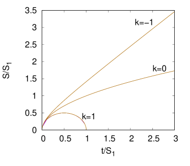
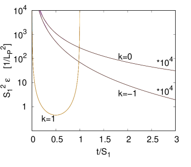
Figure 1: The rescaled scale function (left) and energy density (right) in the solutions with a Small Bang singularity as a function of the scaled time for $k=0,\pm 1$. In the right figure the $k=0$ and $k=-1$ lines are multiplied by $10000$. Each line in the figures is actually six lines on top of each other for $S_{1}$ changing from $10^{-1}$ to $10^{4}$ for the same $k$. The universe recollapses for $k=1$, but expands forever for $k=0,-1$.

The mean curvature in all the three cases $k=0,\pm 1$ is strictly monotonically decreasing (hence it can indeed be used as a correct time coordinate, the ‘York time’), and it shows similar universal, scaling character. In case of $k=0$ even the $S_{1}$ dependence disappears (see equation (3.15)). The Higgs field also has this scaling property in its first two orders:

$$\sqrt{\frac{\kappa}{6}}\Phi(t)-1=S^{2}_{1}\Bigl{(}\!\!\!\! -\!\!\!\! \frac{2}{5}\bigl{(}3\frac{\lambda}{\kappa}+\mu^{2}+\frac{\Lambda}{3}\bigr{)}(\frac{t}{S_{1}})^{2}-\frac{4}{35}\bigl{(}3\frac{\lambda}{\kappa}+\mu^{2}+\frac{\Lambda}{3}\bigr{)}k(\frac{t}{S_{1}})^{3}+$$

$$+\!\!\!\! \frac{2}{15}\bigl{(}3\frac{\lambda}{\kappa}+\mu^{2}+\frac{\Lambda}{3}\bigr{)}\bigl{(}3\frac{\lambda}{\kappa}+\mu^{2}+\frac{\Lambda}{3}-\frac{5}{7}\frac{k^{2}}{S^{2}_{1}}\bigr{)}S^{2}_{1}(\frac{t}{S_{1}})^{4}+{\cal O}(t^{5})\Bigr{)}.$$

However, this scaling property is not showing up in the numerical solutions, because in the third term (where $S_{1}$ shows up without the $1/t$) the numerical coefficient has the same order of magnitude as the previous two. Hence this is not negligible, so already around the Planck time this starts to play an important role, spoiling the scaling behaviour. In (2.2), the equation of motion for the Higgs field, the scale factor appears through the term $\dot{S}/S=\chi/3$. Therefore, since for $k=0$ the mean curvature is independent of $S_{1}$, the time evolution of the Higgs field for $k=0$ is universal, and the numerical solutions confirm this (see Fig. 2).

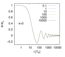
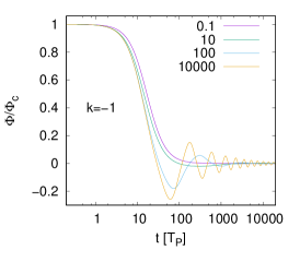
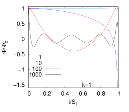
Figure 2: The Higgs field in the solutions with a Small Bang singularity for $k=0,\pm 1$ and for $S_{1}$ changing from $10^{-1}$ to $10^{4}$. In the $k=0$ case $\Phi$ does not depend on $S_{1}$. In the $k=1$ case we use the time coordinate $t/S_{1}$, in which the total ‘lifetime’ of the universe is $1$, independently of $S_{1}$. $\Phi_{c}$ denotes $\sqrt{6/\kappa}$.

5.2 Solutions with a Milne type singularity

In subsection 3.5 we derived the equations for the one-parameter family of solutions with the Milne type singularity. In a neighbourhood of the singularity $\dot{S}=1+{\cal O}(t)$. However, the numerical calculations show that it does not change significantly even on much larger scales, i.e. as far as we can calculate, $S(t)={\cal O}(t)$. If $\phi_{0}>\phi_{0}^{crit}$ (see equation (3.40)) the Higgs field is decreasing with time near $t=0$, but later it oscillates around zero. If $\phi_{0}<\phi_{0}^{crit}$, then the time derivative of the Higgs field is positive but negligible. Thus the Higgs field is although increasing, practically it remains constant.

5.3 Solutions with a Big Bang singularity

In subsection 4.2 we saw that the asymptotic power series solutions with the Big Bang singularity form a 1-parameter family; and for the parameter value $\phi^{2}_{-1/2}$ smaller than $\sqrt{\kappa/12\lambda}$ the discrete parameter $k$ is necessarily 1, for $\phi^{2}_{-1/2}=\sqrt{\kappa/12\lambda}$ it is zero, while for $\phi^{2}_{-1/2}>\sqrt{\kappa/12\lambda}$ it is $-1$. The universe is necessarily recollapsing for $k=1$, in which case the Higgs field diverges (tending either to $\infty$ or $-\infty$) in the ‘Big Crunch’ singularity. The moment of the ‘Big Crunch’ depends on the parameter $\phi^{2}_{-1/2}$ of the solution: The closer the parameter $\phi^{2}_{-1/2}$ to the critical value is, the later the time of the ‘Big Crunch’ is (see Fig. 3).

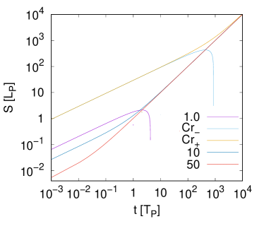
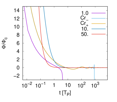
Figure 3: The scale function and the Higgs field as a function of time for various values of the parameter $\phi_{-1/2}$ in solutions with a Big Bang singularity. The discrete parameter $k$ is necessarily $1$ for $\phi^{2}_{-1/2}$ less, and it is $-1$ for $\phi^{2}_{-1/2}$ greater than its critical value $Cr:=\sqrt{\kappa/12\lambda}\simeq 2.054312...$; and $k=0$ for the critical value. Here $Cr_{\pm}:=Cr\pm 0.01$. When $k=0$, then the slope of the scale function agrees with the slope of the linear part of the scale functions with $\phi_{-1/2}$ close to the critical value. $\Phi_{c}$ denotes $\sqrt{6/\kappa}$.

If $k=0$ or $-1$, then the universe is expanding forever, and the rate of expansion for large proper time is getting to be independent of the parameter of the solution. This behaviour is, indeed, compatible with the asymptotic vanishing of the Higgs field.

5.4 Solutions with initial data on the $\Phi=\sqrt{6/\kappa}$ hypersurface

5.4.1 The strategy of the calculations

In subsection 3.4 we saw that solutions that are regular near the spacelike hypersurface $t=0$ on which $\Phi(0)=\sqrt{6/\kappa}$ holds can be parametrized by two continuous parameters, $S_{0}$ and $S_{1}$, fulfilling the inequalities (3.32), and the discrete parameter $k$ and the sign of $\Pi(0)$, denoted henceforth by $s$. An interesting question is what kind of global solutions can we have with such initial conditions. On the other hand, in the numerical calculations of subsections 5.1–5.3, we followed just the opposite strategy: Starting from the singularity (at $t=0$) of a singular solution we calculated the various quantities at later times $t>0$.

Clearly, the latter strategy can be used to determine the regular initial data for a given solution on a spacelike hypersurface defined e.g. by some specific value of the Higgs field, $\Phi=\Phi_{0}$ for some $\Phi_{0}\geq 0$. (By the gauge freedom $\mathbb{Z}_{2}:\Phi\mapsto-\Phi$ one can always assume that $\Phi_{0}\geq 0$.) In particular, if $(S(t),\Phi(t))$ is a solution of the field equations with an initial singularity at $t=0$ and there is some instant when $\Phi=\Phi_{0}$, then primarily we are interested in the initial data for the solution $(S(t),\Phi(t))$ at the instant when $\Phi$ takes the value $\Phi_{0}$ at first time. Thus, in the present numerical calculations, we use the Higgs field to be the time variable, rather than the mean curvature. (This choice for the time variable was motivated by the investigations of subsection 3.4.) Clearly, at this instant $\dot{\Phi}\leq 0$ holds for solutions developing from a Big Bang type singularity, but in general $\dot{S}>0$ does not necessarily hold. The latter would mean that the universe is still expanding at the instant when $\Phi=\Phi_{0}$. Of course, the set of all the initial data obtained in this way is not quite the set of all the independent data sets in the usual Cauchy problem for the system (or rather the set of the solutions of the field equations): E.g. the Cauchy data sets for those solutions of the field equations in which $\Phi$ remains less than $\Phi_{0}$ are not included; while the initial data for those solutions in which $\Phi$ takes the value $\Phi_{0}$ $n$-times are represented by $n$ different points. The latter can happen if $\Phi$ is not a monotonic function of the proper time $t$ (as we saw such a non-monotonic behaviour on Fig. 3 in subsection 5.3, and an oscillatory behaviour on Fig. 2 in subsection 5.1). Thus, apart from these potential multiple representations of initial states, this set of initial data could be considered as the $\Phi=\Phi_{0}$ surface of the constraint hypersurface of the momentum phase space of the EccH system. We will call them ‘phase diagrams’.

5.4.2 The structure of the set of the initial conditions with $\Phi_{0}=\sqrt{6/\kappa}$

First, for the sake of simplicity, let us consider the case $\Phi_{0}=\sqrt{6/\kappa}$. (Thus, with this choice, we a priori excluded those solutions from our considerations for which the Higgs field remain smaller than $\sqrt{6/\kappa}$. Such are the solutions with Small Bang singularities, in which $\Phi$ takes the value $\sqrt{6/\kappa}$ at the singularity rather than at regular points (see subsection 3.2); and also the solutions with a Milne type singularity for the parameters $\phi_{0}\leq 1$ (see subsections 3.3 and 3.4). In subsection 5.5 we consider three more complicated cases, when $\Phi_{0}<\sqrt{6/\kappa}$.) From the investigations of the regular asymptotic solutions in subsection 3.4 we know that only those points of the $(S_{0},S_{1})$-plane can represent initial values that are on or ‘above’ the straight line $S_{1}=\frac{2}{3}\chi_{c}S_{0}$; or, on or ‘below’ the straight line $S_{1}=-\frac{2}{3}\chi_{c}S_{0}$ (see the second inequality in (3.32)). In the states corresponding to the points of these lines, the canonical momentum $\Pi$ is vanishing. For the sake of simplicity, we discuss only the case $S_{1}\geq\frac{2}{3}\chi_{c}S_{0}$. Hence, for each of the cases $k=0,\pm 1$, the set of the initial conditions for the solutions with $S_{1}>0$ consists of two copies of the piece $S_{1}\geq\frac{2}{3}\chi_{c}S_{0}$ of the $(S_{0},S_{1})$-plane such that these two pieces are identified just along the line $S_{1}=\frac{2}{3}\chi_{c}S_{0}$. The two copies correspond to the two signs $s=\pm 1$ of the canonical momentum $\Pi$ at the $\Phi=\Phi_{0}$ hypersurface (see equation (3.31)). Therefore, the set of all the initial conditions for $\Phi^{2}_{0}=6/\kappa$ and given $k$ is the disjoint union of this set and the analogous one in which $S_{1}<0$. At this point it could perhaps be worth stressing that the actual parameters $S_{0}$ and $S_{1}$ for a given solution $(S(t),\Phi(t))$ (e.g. with a Big Bang type singularity) are read-off from the restriction of the solution to a neighbourhood of the $\Phi=\Phi_{0}$ hypersurface as a regular solution (see subsection 3.4), and these should not be confused with the expansion coefficients of the singular solution itself near the singularity. E.g. the $S_{0}$ for the latter would be zero by assumption.

5.4.3 The ‘phase diagram’ of the solutions with $\Phi_{0}=\sqrt{6/\kappa}$

Using the 1-parameter family of singular solutions with the (power series) Big Bang singularity for $k=0,\pm 1$ or with the Milne type singularity (in which case $k=-1$ and $\phi_{0}>1$), we can determine the value of $(S,\dot{S},\dot{\Phi})$ at the instant when $\Phi=\sqrt{6/\kappa}$ at first time. From these we can read off $S_{0}$, $S_{1}$ and $\phi_{1}$ (see subsection 3.4). However, by equation (3.27), these quantities are not independent, and this equation can be considered as a quadratic algebraic equation for $(S_{1}/S_{0})$. Comparing its solution with the value $(S_{1}/S_{0})$ obtained directly from the numerical solution we can determine the sign $s$. In this way we obtain a 1-parameter family of points in the $(S_{0},S_{1})$-plane corresponding to the solutions with (power series) Big Bang singularity in all the three cases $k=0,\pm 1$; and another one corresponding to solutions with the Milne type singularity. In all the solutions with the Big Bang singularity we found $s=-1$ (or, more precisely, $s$ is typically between $-0.99$ and $-1.01$, although the numerical uncertainties near the limit line is greater); but in the Milne case $s$ can be either of $\pm 1$.

The data corresponding to the solutions with Big Bang for the $k=1$ and $k=0$ cases can be drawn on the same diagram; and those with Big Bang with $k=-1$ and with Milne type singularity on another one (see Fig. 4).

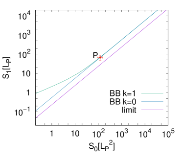
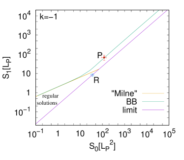
Figure 4: The $(S_{0},S_{1})$-plane of the initial conditions for the solutions with a Big Bang (BB) or Milne type singularity with $k=0,1$ (left figure) and $k=-1$ (right figure) at the moment when $\Phi=\sqrt{6/\kappa}$ at first time. All solutions correspond to points above the (purple) limiting straight line. The data for solutions with a (power series) Big Bang singularity are only on the $s=-1$ copy of the $(S_{0},S_{1})$-plane. For the initial data corresponding to solutions with a Milne type singularity $k=-1$ but $s=\pm 1$. The 1-parameter family of these initial data on the $s=1$ and $s=-1$ copies of the $(S_{0},S_{1})$-plane coincide, and the one on the $s=1$ copy is continued in the other on the $s=-1$ copy. The points between the two Milne lines on the $s=-1$ and $s=1$ sheets, including the limit line (and the point $R$ on it), are initial conditions for regular solutions. Possibly apart from points of a subset of measure zero, all the other points appear to correspond to singular solutions in which the singularity cannot be reached asymptotically by a power series. Such an initial state is represented by the point $P$ on the $s=1$ sheet.

In case of solutions with a power series Big Bang type singularity (see subsection 4.2), as the parameter $\phi^{4}_{-1/2}$ of the asymptotic power series solution increases towards its critical value $\kappa/12\lambda$, the corresponding values of $(S_{0},S_{1})$ on the ‘phase diagram’ tend to infinity. This regime of the parameter, $\phi^{4}_{-1/2}<\kappa/12\lambda$, corresponds to $k=1$ (see Fig. 4, left panel). The critical value of this parameter, $\phi^{4}_{-1/2}=\kappa/12\lambda$, corresponds to another 1-parameter family of solutions. For these solutions $k=0$, and in the $(S_{0},S_{1})$-plane they form a straight line that is the asymptote of the family of the $k=1$ data sets. This line appears to be parallel with the limit straight line $S_{1}=\frac{2}{3}\chi_{c}S_{0}$. In fact, in subsection 4.2 we saw that, near the singularity, the solution with $k=0$ depends on the parameter in a trivial way: The parameter is a simple overall scale factor. The numerical calculations show that this feature remains characteristic even on a much larger scale.

After passing the critical value $\kappa/12\lambda$ of the parameter $\phi^{4}_{-1/2}$ (and hence when already $k=-1$) the corresponding initial values draw the same (at least numerically indistinguishable) line on the $(S_{0},S_{1})$-plane (see Fig. 4, right panel). However, in the domain $\phi^{4}_{-1/2}>\kappa/12\lambda$ of the parameter the values $(S_{0},S_{1})$ are decreasing with increasing $\phi^{4}_{-1/2}$. As we already noted, the initial data for any solution with power series Big Bang singularity are on the $s=-1$ copy of the $(S_{0},S_{1})$-plane.

Next, let us consider the initial data for solutions with a Milne type singularity (see subsection 3.5). As the parameter $\phi_{0}$ of the asymptotic solutions tends from below to a special value $\phi_{0}^{0}$ (whose value, up to numerical uncertainties, is between $1.9$ and $2.1$), the corresponding curve is on the $s=1$ copy of the $(S_{0},S_{1})$-plane, and it approaches the limiting line $S_{1}=\frac{2}{3}\chi_{c}S_{0}$. Increasing $\phi_{0}$ further and passing the special value $\phi_{0}^{0}$, the curve continues on the $s=-1$ copy of the $(S_{0},S_{1})$-plane (see Fig. 4, right panel). The numerical calculations show that, on the $s=-1$ copy, the Milne line is an asymptote of the Big Bang line when $S_{0}\rightarrow 0$.

Finally, note that for $k=-1$ there are regular solutions, i.e. which do not have a singularity neither in the future nor in the past direction. The corresponding points on the ‘phase diagram’ are between the two Milne lines (i.e. for which $s=-1$ and $s=1$), including the limit straight line $S_{1}=\frac{2}{3}\chi_{c}S_{0}$. In particular, the point $R$ corresponds to the special regular solution with initial data $(S_{c}^{2},2\chi_{c}S^{2}_{c}/3)$, discussed at the end of subsection 3.4 (see Fig. 4, right panel).

5.4.4 An evidence for the existence of non-power series asymptotic solutions

To clarify the nature of the solutions with initial data not lying on the distinguished lines above, let us consider the point $(S_{0},S_{1})=(120.2L_{P}^{2},68.0L_{P})$ of the $(S_{0},S_{1})$-plane, denoted by $P$ on Fig. 4. This corresponds both to the values $\phi^{2}_{-1/2}=1.94$ and $\phi^{2}_{-1/2}=2.2$ of the parameter of the solution with a (power series) Big Bang singularity (with $k=1$ and $k=-1$, respectively) provided $s=-1$. (On the ‘phase diagram’ this point is separated enough from the Milne line, because the numerical error for determining the $(S_{0},S_{1})$ values for a Big Bang solution is definitely less than the parameter distance of the point above from the Milne line.) However, with this initial data at $t=0$ we can solve the evolution equations, both in the past ($t<0$) and future ($t>0$) directions, even for $s=1$, too. The results for all the four possibilities $k=\pm 1$, $s=\pm 1$ are shown in Fig. 5.

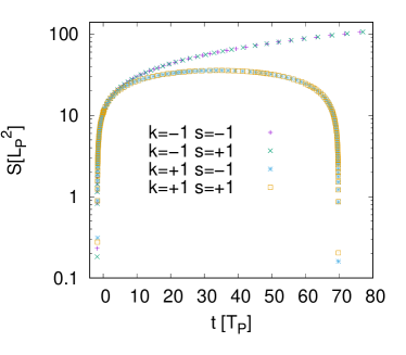
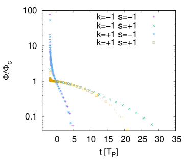
Figure 5: The scale function and the Higgs field, as a function of time (both for $t<0$ and $t>0$), in the numerical solution developed from the initial condition $(S_{0},S_{1})=(120.2L_{P}^{2},68.0L_{P})$ (denoted on Fig. 4, by $P$) at $t=0$ with $k=\pm 1$ and $s=\pm 1$. The plus, the cross, the star and the box denote, respectively, the $(k,s)=(-1,-1)$, the $(-1,1)$, the $(1,-1)$ and the $(1,1)$ cases. $\Phi_{c}$ denotes $\sqrt{6/\kappa}$.

The left panel of Fig. 5 shows the time evolution of the scale function $S$. This function appears to be independent of the sign of $s$ (which is true for all other initial points from the Big Bang line that we studied). On the other hand, in the right panel, we can see that while for $s=-1$ and $k=\pm 1$ the Higgs field $\Phi$ smoothly diverges as $t$ decreases from zero, but for $s=1$ and $k=\pm 1$ we get an abrupt increase of $\Phi$ just below $t=0$ (though the two solutions for $k=1$ and $k=-1$ are different). These solutions start with $S=0$ (at some $t<0$) and a value of $\Phi$ which is finite or infinite (although the numerical calculations indicate that it is probably infinite). If this starting value of $\Phi$ were finite, then the solutions would be of Milne type. However, this could be possible only if some Milne type singularity could not be reached by a power series type asymptotic solution, because their initial values $(S_{0},S_{1})$ are not on the Milne line. Similarly, if for $s=1$ these solutions started with $S=0$ and $\Phi=\infty$, then these solutions could not have power series Big Bang singularities either, because for them $s=-1$ would hold. Therefore, we obtained an example for a solution with either a Milne or (probably) Big Bang type singularity in which the singularity cannot be reached by a power series (‘non-analytic Big Bang’).

5.4.5 The nature of solutions with a generic initial data with $\Phi_{0}=\sqrt{6/\kappa}$

Finally, let us discuss what kind of solutions do we obtain from a generic point (above the limiting line) of the $(S_{0},S_{1})$-plane. It turned out that the singular or non-singular nature of the solutions is independent of the sign of $s$. In particular, if $k=1$, then all the solutions appear to start and end in a singularity. (We inspected solutions with sixteen randomly chosen initial data sets on the $(S_{0},S_{1})$-plane.) In addition to the line indicated on the left panel of Fig. 4 (representing a 1-parameter family of solutions with power series type Big Bang singularity), there may be more such lines. They would correspond to multiple representations of solutions with power series type Big Bang singularity (see the remark at the end of subsection 5.4.1). The rest of the two dimensional allowed subset of the two copies of the $(S_{0},S_{1})$-plane appears to correspond to solutions which are non-analytic around their singularity.

If $k=0$, then all the solutions appear to start ($S_{1}>0$) or end ($S_{1}<0$) in a singularity. The line corresponding to solutions with power series type Big Bang singularity is a straight line (see the left panel of Fig. 4). The rest of the two dimensional allowed subset of the $(S_{0},S_{1})$-plane seems to correspond to solutions which are non-analytic around their singularity.

If $k=-1$, then either a solution is regular everywhere, or it starts or ends in a singularity. The union of the ‘wedges’ between the Milne-line and the limiting line on the $s=1$ and $s=-1$ copies of the $(S_{0},S_{1})$-plane contains initial data for the regular solutions (see the right panel of Fig. 4). In particular, the special solution with the data $(S_{0},S_{1})=(S^{2}_{c},\frac{2}{3}\chi_{c}S^{2}_{c})$ (denoted by $R$ on Fig. 4, right panel) is regular. Indeed, the fact that the boundary of the set of initial data for the regular solutions is just the Milne line could be expected: The Milne singularity is a singularity only of the solution, but not of the spacetime geometry (see subsections 3.3 and 3.5). All the points outside this open set appear to represent initial data for singular solutions; and, apart from the lines corresponding to solutions with a power series Big Bang or Milne type singularity, these are non-analytic around the singularities.

5.5 Solutions with initial data on hypersurfaces with $\Phi<\sqrt{6/\kappa}$

5.5.1 The structure of the set of the initial conditions with $\Phi_{0}<\sqrt{6/\kappa}$

Choosing $\Phi_{0}$ in the definition of the initial hypersurface (of subsection 5.4.1) to be less than $\sqrt{6/\kappa}$, e.g. to be $\frac{1}{2}\sqrt{6/\kappa}$, $\frac{3}{5}\sqrt{6/\kappa}$ or $\frac{4}{5}\sqrt{6/\kappa}$ (as in the following numerical calculations), we include initial data for solutions with (power series) Small Bang singularities in our set of initial conditions, too. This makes the ‘phase diagram’ of the solutions slightly more complicated, but the analysis of subsections 5.4.2–5.4.4 can be repeated.

In fact, for given $\Phi=\Phi_{0}$ the value of $S$, $\dot{S}$ and $\dot{\Phi}$ are not independent, because they must satisfy the constraint in (2.1) (together with the expression (2.3) for the energy density). This yields the second order algebraic equation

$$\dot{\Phi}^{2}+2\Phi_{0}\bigl{(}\frac{\dot{S}}{S}\bigr{)}\dot{\Phi}+\Phi_{0}^{2}\bigl{(}\mu^{2}+\frac{\Lambda}{3}+\frac{1}{2}\lambda\Phi^{2}_{0}\bigr{)}-(\frac{6}{\kappa}-\Phi^{2}_{0})\Bigl{(}\bigl{(}\frac{\dot{S}}{S}\bigr{)}^{2}+\frac{k}{S^{2}}-\frac{\Lambda}{3}\Bigr{)}=0$$ (5.1)

for $\dot{\Phi}$. To have a solution of this equation, its discriminant must be non-negative,

$$D:=\frac{6}{\kappa}\bigl{(}\frac{\dot{S}}{S}\bigr{)}^{2}-\Phi^{2}_{0}\bigl{(}\mu^{2}+\frac{\Lambda}{3}+\frac{1}{2}\lambda\Phi^{2}_{0}\bigr{)}+(\frac{6}{\kappa}-\Phi^{2}_{0})\Bigl{(}\frac{k}{S^{2}}-\frac{\Lambda}{3}\Bigr{)}\geq 0,$$ (5.2)

in which case the solution of (5.1) is

$$\dot{\Phi}=-\Phi_{0}(\frac{\dot{S}}{S})\pm\sqrt{D}.$$ (5.3)

The sign in front of $\sqrt{D}$ will be denoted by $s$.

For a given $\Phi^{2}_{0}$ condition (5.2) could be a non-trivial constraint, but for a different $\Phi^{2}_{0}$ it could be satisfied identically. In particular, for $\Phi^{2}_{0}=6/\kappa$ condition (5.2) reduces to the second inequality in (3.32), in which case it is independent of the discrete parameter $k$; and the boundary $D=0$ of the initial conditions for solutions, i.e. the limit line, is a straight line on the $(S,\dot{S})$-plane. However, for $\Phi^{2}_{0}\not=6/\kappa$ this condition depends on the value of $k$, and the boundary $D=0$ is given by

$$\dot{S}^{2}=-k(1-\frac{\kappa}{6}\Phi^{2}_{0})+\bigl{(}\frac{\kappa}{6}\mu^{2}\Phi^{2}_{0}+\frac{\kappa\lambda}{12}\Phi^{4}_{0}+\frac{\Lambda}{3}\bigr{)}S^{2}.$$ (5.4)

Here we do not give the exhaustive discussion of the quite diverse possibilities, simply we illustrate some of them by a few examples. The detailed analysis is elementary and straightforward. In particular, for $k=0$ (5.4) gives two straight lines on the $(S,\dot{S})$-plane through the origin, and the coefficient of $S^{2}$ on the right hand side is positive precisely when either

$$\lambda\Phi^{2}_{0}<-\mu^{2}-\sqrt{\mu^{4}-4\Lambda\lambda/\kappa}\hskip 20.0pt{\rm or}\hskip 20.0pt-\mu^{2}+\sqrt{\mu^{4}-4\Lambda\lambda/\kappa}<\lambda\Phi^{2}_{0}.$$ (5.5)

Thus, if $\lambda\Phi_{0}^{2}$ is chosen to satisfy (5.5), then only those points of the $(S,\dot{S})$-plane with $\dot{S}\geq 0$ can represent initial data that are on or ‘above’ the limit line. Any of our present choice for $\Phi^{2}_{0}$ will be much bigger than $(-\mu^{2}+\sqrt{\mu^{4}-4\Lambda\lambda/\kappa})/\lambda$, and hence (5.2) is a non-trivial constraint with a non-trivial limit (straight) line (see e.g. Fig. 6, right panel). Therefore, the set of the initial data with $\dot{S}\geq 0$ consists of two copies of the part of the $(S,\dot{S})$-plane ‘above’ the limit line, labelled by the two signs $s=\pm 1$, which copies are identified along the limit line.

For $k=1$ and $\Phi^{2}_{0}$ making the coefficient of $S^{2}$ in (5.4) positive, (5.4) gives a nontrivial limit curve for any $S^{2}$ only for $\Phi^{2}_{0}>6/\kappa$; but for $\Phi^{2}_{0}<6/\kappa$ (as in our case), the limit curve starts from the point $(S_{\bullet},0)$ both in the $\dot{S}>0$ and $\dot{S}<0$ half planes, where

$$S^{2}_{\bullet}:=2\frac{6-\kappa\Phi^{2}_{0}}{\kappa\lambda\Phi^{4}_{0}+2\kappa\mu^{2}\Phi^{2}_{0}+4\Lambda}.$$

In this case the $(S,\dot{S})$-plane does not split into the two disjoint pieces $\dot{S}>0$ and $\dot{S}<0$, they join together along the line between the points $(0,0)$ and $(S_{\bullet},0)$. The set of all the initial data consists of two such copies, labelled by the sign $s=\pm 1$, which are identified along their limit curves (see e.g. Fig. 6, middle panel).

If $k=-1$, then an analogous analysis yields that, for $\Phi^{2}_{0}<6/\kappa$ but making the coefficient of $S^{2}$ in (5.4) positive, the limit curve has two disconnected branches (one in the $\dot{S}>0$ and the other in the $\dot{S}<0$ half-plane), exists for any $S>0$, and they start at $(0,\pm\sqrt{1-\kappa\Phi^{2}_{0}/6})$. The set of all the initial data with $\dot{S}>0$ consists of two copies of the points on or ‘above’ the limit curve, labelled by the sign $s=\pm 1$, which are identified along their limit curves (see e.g. Fig. 6, left panel). The set of all the initial data is the disjoint union of this set and the one with $\dot{S}<0$.

5.5.2 The ‘phase diagram’ of the solutions with $\Phi_{0}<\sqrt{6/\kappa}$

Similarly to subsection 5.4.3, starting from the singularity of a singular solution, we determine the initial data on the spacelike hypersurface specified by the condition that $\Phi$ takes the value $\Phi_{0}=\frac{1}{2}\sqrt{6/\kappa}$, or $\frac{3}{5}\sqrt{6/\kappa}$, or $\frac{4}{5}\sqrt{6/\kappa}$ for the first time. Now, to parametrize these solutions, we still use the parameters appearing in their asymptotic form near the singularity (and discussed in subsections 3.2, 3.5 and 4.2). Comparing the solution (5.3) with the value $(\dot{S}/S)$ obtained directly from the numerical solution we can determine the sign $s$. In this way, in any of the three choices for $\Phi_{0}$, we obtain 1-parameter families of points in the $(S,\dot{S})$-plane corresponding to solutions with the (power series) Big Bang (BB) and Small Bang (SB) singularities in all the three cases $k=0,\pm 1$; and a 1-parameter family of points corresponding to solutions with the Milne type singularity (with $k=-1$). (The exceptional solution of subsection 3.3 corresponds to a single point on the Milne line.) The results are shown, in the $\Phi_{0}=\frac{1}{2}\sqrt{6/\kappa}$, $\frac{3}{5}\sqrt{6/\kappa}$ and $\frac{4}{5}\sqrt{6/\kappa}$ cases, respectively, by Fig. 6, Fig. 7 and Fig. 8.

We saw that for $\Phi_{0}=\sqrt{6/\kappa}$ the Big Bang lines in the $k=1$ and $k=-1$ cases on the $(S_{0},S_{1})$-plane (numerically) coincided, for $k=0$ this was a straight line through the origin, and in all these cases we obtained $s=-1$. For any solutions with a power series Big Bang singularity $s=-1$ still holds even for $\Phi_{0}<\sqrt{6/\kappa}$, and, for $k=0$, this is still a straight line, but these lines for $k=-1$ and $k=1$ do not coincide any more. In addition to this, the only essential, qualitative difference between the $\Phi_{0}=\sqrt{6/\kappa}$ and the present cases is that now solutions with Small Bang singularities are present, and the parameter domain for the solutions with a Milne type singularity is enlarged. Thus, we discuss only these in detail.

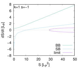
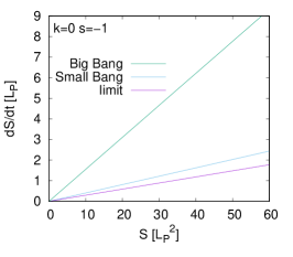
Figure 6: The ‘phase diagram’ for $\Phi_{0}=\frac{1}{2}\sqrt{6/\kappa}$ and $k=-1,1$ and $0$, respectively. BB is the Big Bang, and SB is the Small Bang line.

Solutions with a Milne singularity exist only for $k=-1$, and the main qualitative properties of the Milne line in the present $\Phi_{0}<\sqrt{6/\kappa}$ cases appear to be the same that we saw when $\Phi_{0}$ was $\sqrt{6/\kappa}$ (see the left panel of Fig. 6, Fig. 7 and Fig. 8). The only new phenomenon is that the exceptional solution (with asymptotics discussed in subsection 3.3 and corresponding to the parameter $\phi_{0}=1$), a special member of the Milne family, appears: For $\Phi_{0}=\frac{4}{5}\sqrt{6/\kappa}$ the corresponding point in the ‘phase diagram’ is on the $s=1$ copy of the $(S,\dot{S})$-plane (see Fig. 8), and decreasing $\Phi_{0}$ to tend to $\frac{1}{2}\sqrt{6/\kappa}$ this point seems to tend to the limit line (see Fig. 6). For smaller $\Phi_{0}$ we expect this point to be already on the $s=-1$ copy of the $(S,\dot{S})$-plane.

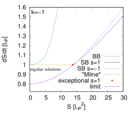
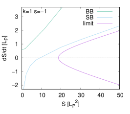
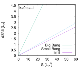
Figure 7: The ‘phase diagram’ for $\Phi_{0}=\frac{3}{5}\sqrt{6/\kappa}$ and $k=-1,1$ and $0$, respectively. The Big Bang (BB) line is on the $s=-1$ copy of the $(S,\dot{S})$-plane. SB is the Small Bang line.

However, the initial data for solutions with a (power series) Small Bang singularity have much more complicated structure. First, for $k=-1$ the Small Bang line tends asymptotically, in the $S_{1}\rightarrow 0$ limit, to the initial data for the exceptional solution, but, in contrast to the Big Bang line, it is not confined into the $s=-1$ copy of the $(S,\dot{S})$-plane: If $\Phi_{0}=\frac{1}{2}\sqrt{6/\kappa}$, then the Small Bang line is in the $s=-1$ copy, but for greater $\Phi_{0}$ it starts (asymptotically) from the point for the exceptional solution on the $s=1$ leaf, crosses the limit line, and then continues on the $s=-1$ leaf (see the left panel of Fig. 6, Fig. 7 and Fig. 8).

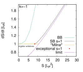
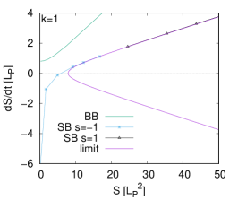
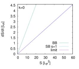
Figure 8: The ‘phase diagram’ for $\Phi_{0}=\frac{4}{5}\sqrt{6/\kappa}$ and $k=-1,1$ and $0$, respectively. The Big Bang (BB) line is on the $s=-1$ copy of the $(S,\dot{S})$-plane. SB is the Small Bang line.

If $k=1$, then, as we saw in subsection 5.5.2, the ‘phase diagram’ is connected, it does not split into the disjoint pieces $\dot{S}>0$ and $\dot{S}<0$. In fact, for any of the given values for $\Phi_{0}<\sqrt{6/\kappa}$, a piece of the Small Bang line is in the $\dot{S}<0$ domain, another is in the $\dot{S}>0$ domain, and there is an initial state in which $\dot{S}=0$. This latter is the data for the solution in which the universe starts to recollapse just when the Higgs field takes the value $\Phi_{0}$. The piece of the Small Bang line in the $\dot{S}<0$ domain is on the $s=-1$ copy of the $(S,\dot{S})$-plane. Increasing $\Phi_{0}$ to tend to $\sqrt{6/\kappa}$, the Small Bang line is getting to be closer and closer to the limit line. After crossing the limit line, the Small Bang line continues on the $s=1$ leaf (see the middle panels of Fig. 6, Fig. 7 and Fig. 8).

As we saw in subsection 3.2, for $k=0$ the parameter $S_{1}$ is only an overall scale factor of the asymptotic solution, and the Higgs field is independent of $S_{1}$. The numerical calculations demonstrate this behaviour on a much larger scale, independently of the value of $\Phi_{0}$: On the $(S,\dot{S})$-plane the line corresponding to these solutions is a straight line through the origin (see the right panels). On the other hand, the slope of the Small Bang straight line depends on the value of $\Phi_{0}$: Increasing $\Phi_{0}$ to tend to to $\sqrt{6/\kappa}$, the Small Bang line is getting to be closer and closer the limit line. For $\Phi_{0}$ less than a special value (which is approximately $0.78\,\sqrt{6/\kappa}$) the Small Bang line is still on the $s=-1$ leaf. but increasing $\Phi_{0}$ further it is already on the $s=1$ leaf (see the right panels of Fig. 6, Fig. 7 and Fig. 8).

Apart from the domains for the regular solutions and the lines corresponding to solutions with (Big Bang, Small Bang or Milne type) singularities that can be reached by power series, the points correspond to initial values for singular solutions that are not analytic near their singularity.

6 Conclusions and summary

We investigated the Einstein–conformally coupled Higgs field (EccH) system in the presence of Friedman–Robertson–Walker symmetries both analytically (near the initial singularities) and numerically. We determined analytically all the asymptotic, power series solutions up to fourth order near the singularities. We found three 1-parameter families of solutions. In the first both the Higgs field and certain scalar polynomial curvature invariants diverge (Big Bang), in the second the Higgs field remain bounded but certain scalar polynomial curvature invariants diverge (Small Bang), and in the third both the Higgs field and the curvature invariants remain bounded. In fact, while the first two are genuine physical spacetime singularities; the third is only a Milne type singularity, and the spacetime can be extended to a bigger one through this. The existence of these singular solutions demonstrates that the symmetry breaking instantaneous vacuum states of the Higgs sector are not only kinematical possibilities, but that, as it was claimed in [3], they do emerge non-trivially during the dynamics of the system.

We determined these solutions numerically, starting from the sub-Planck scale to the era of the weak interactions, as well. We found that the asymptotic, power series solutions above give surprisingly good approximation even on this scale. Also, we investigated numerically the generic properties of the set of the initial data of the EccH system. The solutions with the Big Bang, Small Bang and Milne type singularities above turned out to form only a subset of measure zero in the set of all the initial conditions. The complement of these is the union of the set of initial conditions for the regular solutions (with $k=-1$), and that for singular solutions that cannot be expanded in power series near the singularities.

Gy. Wolf was supported by the Hungarian OTKA fund K109462.

References

- [1] S. W. Hawking, G. F. R. Ellis, The Large Scale Structure of Spacetime, Cambridge University Press, Cambridge 1973
- [2] E. S. Abers, B. W. Lee, Gauge theories, Phys. Rep. 9 1–141 (1973)
- [3] L. B. Szabados, Gravity, as a classical regulator for the Higgs field, and the genesis of rest masses and electric charge, arXiv: 1603.06997v3 L. B. Szabados, On gravity’s role in the genesis of rest masses of classical fields, Gen. Relat. Grav. (2018) 50 34, DOI:10.1007/s10714-018-2340-1, arXiv: 1802.04401
- [4] G. F. R. Ellis, B. G. Schmidt, Singular spacetimes, Gen. Rel. Grav. 8 915-953 (1977)
- [5] W. H. Press, S. A. Teukolsky, W. T. Vetterling, B. P. Flannery, Numerical Recipies in Fortran Cambridge University Press, 1992