Microscopy for Atomic and Magnetic Structures Based on Thermal Neutron Fourier-transform Ghost Imaging

Abstract

We present a lensless, Fourier-transform ghost imaging scheme by exploring the fourth-order correlation function of spatially incoherent thermal neutron waves. This technique is established on the Fermi-Dirac statistics and the anti-bunching effect of fermionic fields, and the analysis must be fully quantum mechanical. The spinor representation of neutron waves and the derivation purely from the Schrödinger equation makes our work the first, rigorous, robust and truly fermionic ghost imaging scheme. The investigation demonstrates that the coincidence of the intensity fluctuations between the reference arm and the sample arm is directly related to the lateral Fourier-transform of the longitudinal projection of the sample’s atomic and magnetic spatial distribution. By avoiding lens systems in neutron optics, our method can potentially achieve de Broglie wavelength level resolution, incomparable by current neutron imaging techniques. Its novel capability to image crystallined and noncrystallined samples, especially the micro magnetic structures, will bring important applications to various scientific frontiers.

Ever since the discovery of the Hanbury Brown and Twiss (HBT) effectBrown and Twiss (1956a, b), the quantum statistical properties of bosonic and fermionic fields have been intensively investigated. It is found that the intensity correlation in HBT measurements actually originates from the photon bunching of thermal light sources. In parallel, a distinctive antibunching effect, with its deep roots in the Pauli exclusive principle, was predicted for fermionsSilverman (1987a, b); Tyc (1998), and subsequently observed in free thermal neutronsIannuzzi et al. (2006, 2011), free electronsKlesel et al. (2002), two dimensional electron gas of semiconductor systemsHenny et al. (1999); Oliver et al. (1999), and free fermionic atoms released from an optical lattice.Rom et al. (2006).

Over the past two decades the bosonic bunching property has led to an imaging methodology, called quantum imaging or synonymously ghost imaging (GI), by exploring the intensity correlation between split beams. It was first realized with entangled photon pairs generated by spontaneous parametric down conversion from a nonlinear crystalD’Angelo et al. (2001). Further developments demonstrated that quantum entanglement was unnecessaryBennink et al. (2002) and thermal light could also be employedCheng and Han (2004); Gatti et al. (2004). Moreover, such a concept is directly expandable to the de Broglie waves of massive particlesKhakimov et al. (2016).

Essentially a nonlocal imaging scheme, GI provides vast flexibility in optical system design without requiring a lens system for focusing and magnification, and has wide applications from long range remote-sensingZhao et al. (2012); Hardy and Shapiro (2013) to short range microscopyAspden et al. (2015). Different from conventional methods, the light field transmitted through or reflected by a sample is recorded only with a non-spatially resolving detector (i.e., a bucket or point detector), while the spatial profile is recorded by a high-resolution reference detector. From the Fourier-transform diffraction pattern collected at the Fresnel region, the sample structure can be successfully reconstructedZhang et al. (2007). In latest developments, hard x-ray GI was achieved experimentally by employing synchrotron radiationYu et al. (2016); Pelliccia et al. (2016). Theoretically the spatial resolution of lensless Fourier-transform GI is only limited by the wavelength and provides the potential to achieve atomic-resolution imaging of noncrystalline samples using laboratory x-ray sourcesYu et al. (2016). The quantum waves of massive bosons were brought into GI as well. Correlated metastable helium atom pairs, extracted from a Bose-Einstein condensate, were shown to be capable of generating a 2D imaging of a target with submillimeter resolutionKhakimov et al. (2016).

As a major achievement of modern physics, thermal neutron scattering has greatly enriched our understanding of atomic-scale structures and dynamical properties of materialsSquires (1996); Lovesey (1984). With de Broglie wavelength at the same order of interatomic distances in solids and liquids, carrying no net charge, and participating nuclear scattering and magnetic scattering, thermal neutrons make an ideal probe for detecting matter’s atomic and magnetic structures. Among all subfields of neutron science, neutron attenuation imaging, phase imaging and holography have been under intense developement and created a variety of important toolsAnderson et al. (2009). The latest, state-of-the-art neutron microscopy, by employing multi-layered Wolter mirrors, not only focuses the neutron beam onto the target, but also magnifies the imageLiu et al. (2013). Tweenty micron resolution has been achieved while a potential resolution of 1 micron is reachable if phase contrast information is further incoporated, though still orders of magnitude larger than the wavelength.

Thermal neutrons and hard x-rays have similar wavelength range. As x-rays are mostly scattered by the electric field of electrons, they are suitable for studying atomic structures comprised of heavy elements, but incapable of probing magnetic structures. Complementary to x-rays, thermal neutrons are sensitive to the nuclear scattering of light-elements and the magnetic scattering of unpaired electrons. Thus, a thermal neutron GI technique can greatly improve the resolving power of seeing through matter’s atomic and magnetic structures. However, due to the complexity in calculating the fourth-order correlation function of neutron scattering processes, particularly when involving neutron’s magnetic moment, GI employing thermal neutron probe has yet to be developed. Here for the first time in literature, we present a Fourier-transform imaging scheme for atomic and magnetic structures based on the neutron quantum coincidence in a GI setup.

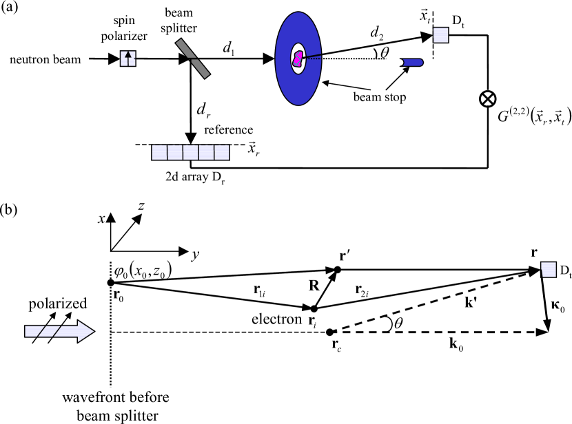
Figure 1: Illustration of thermal neutron ghost imaging. (a) Schematic experimental setup. A polarized (in $\hat{z}$ dirction), spatially incoherent thermal neutron beam is divided into a sample arm and a reference arm. An extra beam-stop shield is inserted around the sample to remove the incident waves, while the sample is mounted in the opening window of the screen. (b) The definitions of the coordinate system and the vectors used in the calculations, the angles are exaggerated: $\mathbf{r}_{0}$ one point on the source wavefront, $\mathbf{r}_{i}$ the $i$-th unpaired electron, $\mathbf{r}$ the detector, $\mathbf{r^{\prime}}$ a magnetic field point, $\mathbf{r}_{c}$ the system center.

In GI, the particle flux is divided into two by a beamsplitter, one reference arm and one sample arm (Fig. 1a). The coincidence rate at these two detectors is proportional to the fourth-order correlation function of the quantum fields,

$$G^{(2,2)}(\bm{\xi}_{r},\bm{\xi}_{t})=\left<\psi^{\dagger}(\bm{\xi}_{r})\psi^{\dagger}(\bm{\xi}_{t})\psi(\bm{\xi}_{t})\psi(\bm{\xi}_{r})\right>,$$ (1)

where $\left<\cdot\cdot\cdot\right>$ means the ensemble average, and we use Greek symbol $\bm{\xi}=(x,z)$ to label the 2d transverse coordinate of the wavefront. $\bm{\xi}_{r}$ and $\bm{\xi}_{t}$ are for the reference and target detectors, respectively. The propagation of quantum field is governed by

$$\psi(\bm{\xi})=\int h(\bm{\xi},\bm{\eta})\varphi(\bm{\eta})d\bm{\eta},$$ (2)

where $\varphi$ and $\psi$ are the source and output fields, respectively; $h(\bm{\xi},\bm{\eta})$ is the impulse response function, and $\bm{\eta}$ labels the transverse coordinate of the wavefront at the source. The statistical properties of $\psi$ and $\varphi$ are bridged by the function $h(\bm{\xi},\bm{\eta})$. Theory has shown that on the source wavefrontTyc (1998); Gan et al. (2009); Goodman (1985)

$$G^{(2,2)}(\bm{\eta}_{1},\bm{\eta}_{1}^{\prime},\bm{\eta}_{2},\bm{\eta}_{2}^{\prime}) =G^{(1,1)}(\bm{\eta}_{1},\bm{\eta}_{2}^{\prime})G^{(1,1)}(\bm{\eta}_{1}^{\prime},\bm{\eta}_{2})$$ (3)

$$\pm G^{(1,1)}(\bm{\eta}_{1},\bm{\eta}_{2})G^{(1,1)}(\bm{\eta}_{1}^{\prime},\bm{\eta}_{2}^{\prime}),$$

where $G^{(1,1)}(\bm{\eta},\bm{\eta^{\prime}})$ is the second-order correlation function of the source field, defined as $G^{(1,1)}(\bm{\eta},\bm{\eta^{\prime}})=\left<\psi^{\dagger}(\bm{\eta})\psi(\bm{\eta^{\prime}})\right>$. In Eq. (3), the positive (negative) sign imply the bunching (antibunching) effect for bosons (fermions). Further , after introducing a quantity named intensity fluctuation, $\Delta I(\bm{\xi})=I(\bm{\xi})-\left<I(\bm{\xi})\right>$, from Eqs. (1)-(3) the correlation between the intensity fluctuations at the two detectors becomesCheng and Han (2004)

$$\left<\Delta I_{r}(\bm{\xi}_{r})\Delta I_{t}(\bm{\xi}_{t})\right>=$$

$$\quad\pm v_{i}v_{f}\left|\int d\bm{\eta}d\bm{\eta^{\prime}}G^{(1,1)}(\bm{\eta},\bm{\eta}^{\prime})h^{*}_{r}(\bm{\xi}_{r},\bm{\eta})h_{t}(\bm{\xi}_{t},\bm{\eta}^{\prime})\right|^{2}.$$ (4)

Here, the initial and final velocities $v_{i}$ and $v_{f}$ are included for massive particles.

We consider an incident neutron field with a fully spatially incoherent wavefront,

$$G^{(1,1)}(\bm{\eta},\bm{\eta}^{\prime})=\left<\varphi^{\dagger}(\bm{\eta})\varphi(\bm{\eta}^{\prime})\right>=I_{0}\delta(\bm{\eta}-\bm{\eta}^{\prime}),$$ (5)

where $I_{0}$ is the beam intensity per unit area. In fact, it is this pattern that encodes the wavefront and makes coincidence imaging possible. With Eq. (5), the calculation of Eq. (4) is essentially reduced to the derivation of $h_{r}(\bm{\xi}_{r},\bm{\eta})$ and $h_{t}(\bm{\xi}_{t},\bm{\eta})$.

We consider quasimonochromatic and noninteracting thermal neutrons with spin polarized in the $\hat{z}$ direction. The coordinate system is defined in Fig. 1b. The incident neutron wave function after the beamsplitter*[SeeSupplementalMaterialat][fordetails.]supplemental1

$$\psi_{\text{in}}(\mathbf{r})=\frac{1}{i\lambda}\int d\bm{\eta}\,\varphi(\bm{\eta})\frac{\exp\left(ik\left|\mathbf{r}-\mathbf{r}_{0}\right|\right)}{\left|\mathbf{r}-\mathbf{r}_{0}\right|}\begin{bmatrix}1\\ 0\end{bmatrix}$$ (6)

is an exact solution to the Schrödinger equation with $\varphi(x_{0},z_{0})$ as the field source, where $\bm{\eta}=(x_{0},z_{0})$, and $\lambda$ and $k$ are the wavelength and wavevector, respectively. Immediately, the reference wave is obtained as $\psi_{\text{in}}(\mathbf{r}_{r})$.

However, calculating the neutron wave function at the target detector is challenging. Conventional neutron scattering theory is established on plane wave incidence and invalid for the incidence field in Eq. (6). The interaction between neutron and matter is best described as a potential scattering problem with $V(\mathbf{r^{\prime}})=\sum_{j}V_{j}^{n}(\mathbf{r^{\prime}})+\sum_{i}V_{i}^{m}(\mathbf{r^{\prime}})$ as the potentialSquires (1996). The first summation is over all nuclear sites with the Fermi pseudopotential for the $j$-th nucleus

$$V_{j}^{n}(\mathbf{r^{\prime}})=\frac{2\pi\hbar^{2}}{m_{n}}\left[A_{j}+B_{j}\bm{\sigma}\cdot\mathbf{I}_{j}\right]\delta(\mathbf{r^{\prime}}-\mathbf{r}_{j}),$$ (7)

while the second summation is over all unpaired electron sites with the magnetic potential for the $i$-th electron

$$V_{i}^{m}(\mathbf{r^{\prime}}) = -\frac{\hbar^{2}}{2m_{n}}\gamma r_{e}\bm{\sigma}\cdot\left[\mathbf{W}_{Si}(\mathbf{r^{\prime}})+\mathbf{W}_{Li}(\mathbf{r^{\prime}})\right],$$ (8)

$$\mathbf{W}_{Si}(\mathbf{r^{\prime}}) = \nabla\times\left(\frac{\mathbf{s}_{i}\times\mathbf{\hat{R}}}{R^{2}}\right),\ \mathbf{W}_{Li}(\mathbf{r^{\prime}})=\frac{1}{\hbar}\frac{\mathbf{p}_{i}\times\mathbf{\hat{R}}}{R^{2}}.$$ (9)

In the above equations, $m_{n}$ is the neutron mass, $r_{e}$ the classical radius of electron, $\gamma=1.913$; $A_{j}=\left[\left(I_{j}+1\right)b_{j}^{+}+I_{j}b_{j}^{-}\right]/\left(2I_{j}+1\right)$, $B_{j}=\left[b_{j}^{+}-b_{j}^{-}\right]/\left(2I_{j}+1\right)$, $I_{j}$ is the nuclear spin of the $j$-th nucleus. The neutron plus nucleus can form total spins $I_{j}+\frac{1}{2}$ and $I_{j}-\frac{1}{2}$, and $b_{j}^{+}$ and $b_{j}^{-}$ are the free scattering lengths of the two corresponding eigenstates, respectively. Because coherent nuclear scattering does not change neutron spin, we drop the $B_{j}$ term in this paper to keep our discussion focused. The Pauli matrix $\bm{\sigma}$ in Eq. (8) is the operator for the neutron’s spin. The magnetic field contains two contributions. $\mathbf{W}_{Si}$ arises from the electron’s magnetic moment, whereas $\mathbf{W}_{Li}$ originates from the electron’s orbital movement. $\mathbf{s}_{i}$ and $\mathbf{p}_{i}$ are electron’s spin and momentum operators, respectively; $\mathbf{\hat{R}}$ is the unit vector of $\mathbf{R}$ ($\equiv\mathbf{r^{\prime}}-\mathbf{r}_{i}$) with $\mathbf{r}_{i}$ the electron position.

For simplicity, we restrict our discussion in this paper to elastic scattering only. The following derivation can be easily generalized to include inelastic scattering. Elastic vs inelastic scattering is routinely resolved by means of energy-analyzing crystal at the detector side, where neutrons carrying the incident energy correspond to elastic scattering. We start from the Lippmann-Schwinger integral equationCohen-Tannoudji et al. (2005), i.e.

$$\psi(\mathbf{r})=\psi_{0}(\mathbf{r})+\frac{2m_{n}}{\hbar^{2}}\int d^{3}r^{\prime}G(\mathbf{r}-\mathbf{r^{\prime}})V(\mathbf{r^{\prime}})\psi(\mathbf{r^{\prime}}),$$ (10)

where $\psi_{0}(\mathbf{r})$ is a solution of the homogeneous equation $(\nabla^{2}+k^{2})\psi_{0}(\mathbf{r})=0$ and $G(\mathbf{r}-\mathbf{r^{\prime}})$ is the outgoing Green’s function given by

$$G(\mathbf{r}-\mathbf{r^{\prime}})=-\frac{\exp(ik\left|\mathbf{r}-\mathbf{r^{\prime}}\right|)}{4\pi\left|\mathbf{r}-\mathbf{r^{\prime}}\right|}.$$ (11)

When the potential $V$ is considered a small perturbation, the $\psi$ in the integrand can be approximated by the incident wave function $\psi_{\text{in}}$. Due to $(\nabla^{2}+k^{2})\psi_{\text{in}}(\mathbf{r})\propto\delta(y-y_{0})$, when the sample is far away from the beamsplitter, coordinate $y_{0}$ is considered outside the sample space. Therefore, $\psi_{\text{in}}(\mathbf{r})$ sufficiently satisfies the homogeneous equation and $\psi_{0}(\mathbf{r})$ can be replaced by $\psi_{\text{in}}(\mathbf{r})$ as well. The integral term on the rhs of Eq. (10) is identified as the scattering wave function.

In Fig. 1a polarized neutrons are collected. Under the diffuse illumination (Eq. (5)), neutrons can fly in random directions. Thus for spin-up detection, an extra beam-stop screen is required to remove the incidence wave, and the sample is mounted in the small opening window (Fig. 1a). Substituting Eqs. (7)-(9) and (11) into Eq. (10), under the only assumption that the sample size is much smaller than the source-sample distance $d_{1}$ and the sample-detector distance $d_{2}$, the scattering wave function can be expressed assup

$$\psi^{\text{sc}}_{\nu^{\prime}\nu}(\mathbf{r}) =\frac{i}{\lambda}\int d\bm{\eta}\varphi(\bm{\eta})\int d^{3}r^{\prime}\frac{\exp[ik(r_{1}+r_{2})]}{r_{1}r_{2}}$$ (12)

$$\ \left\{\beta\bm{\sigma}\cdot\left[\bm{\hat{\kappa}}_{c}\times\left(\mathbf{M}(\mathbf{r^{\prime}})\times\bm{\hat{\kappa}}_{c}\right)\right]+A(\mathbf{r^{\prime}})\right\}\begin{bmatrix}1\\ 0\end{bmatrix},$$

where $\left|\nu\right>$ and $\left|\nu^{\prime}\right>$ are the initial and final states of the sample, $A(\mathbf{r^{\prime}})=\left<\nu^{\prime}\left|\sum_{j}A_{j}\delta(\mathbf{r^{\prime}}-\mathbf{r}_{j})\right|\nu\right>$,$\mathbf{M}(\mathbf{r^{\prime}})=\left<\nu^{\prime}\left|\bm{\mathcal{M}}(\mathbf{r^{\prime}})\right|\nu\right>$, $\bm{\mathcal{M}}(\mathbf{r^{\prime}})$ is the operator for the local magnetization, $\beta=\gamma r_{e}/(2\mu_{B})$, $\mathbf{r}_{1}(\mathbf{r^{\prime}},\mathbf{r}_{0})=\mathbf{r^{\prime}}-\mathbf{r}_{0}$, $\mathbf{r}_{2}(\mathbf{r},\mathbf{r^{\prime}})=\mathbf{r}-\mathbf{r^{\prime}}$, $\bm{\kappa}_{c}=k\left[\mathbf{\hat{r}}_{1}(\mathbf{r}_{c},\mathbf{r}_{0})-\mathbf{\hat{r}}_{2}(\mathbf{r},\mathbf{r}_{c})\right]$, and $\mathbf{r}_{c}$ is the center of the sample and $\mathbf{r}_{0}$ a point on the source. $\bm{\kappa}_{c}$ varies when the source point $\mathbf{r}_{0}$ changes.

Now the $h_{r}$ and $h_{t}$ functions are readily extractable from Eqs. (6) and (12). We emphasize that Eq. (12) is valid for all sizes of source and scattering angle $\theta$. In the following discussion, we would focus on the case of small angle scattering with a beam size much smaller than $d_{1}$ and $d_{2}$ so that the paraxial approximation is applicable. The scattering vector $\bm{\kappa}_{c}$ can now be substituted with the conventional $\bm{\kappa}_{0}$, whereas varations of $\bm{\kappa}_{c}$ from $\bm{\kappa}_{0}$ only make negligible corrections. Consequently, $\bm{\kappa}_{0}$ can be taken out of the integrand in Eq. (12). We would like to define the probed sample functions as

$$\begin{bmatrix}S^{\uparrow}(\mathbf{r^{\prime}})\\ S^{\downarrow}(\mathbf{r^{\prime}})\end{bmatrix}=\left\{\beta\bm{\sigma}\cdot\left[\bm{\hat{\kappa}}_{0}\times\left(\mathbf{M}(\mathbf{r^{\prime}})\times\bm{\hat{\kappa}}_{0}\right)\right]+A(\mathbf{r^{\prime}})\right\}\begin{bmatrix}1\\ 0\end{bmatrix}.$$ (13)

Under paraxial condition, we have

$$h_{r}(\bm{\xi}_{r},\bm{\eta})=\frac{e^{ikd_{r}}}{i\lambda d_{r}}\exp\left[\frac{i\pi}{\lambda d_{r}}\left(\bm{\xi}_{r}-\bm{\eta}\right)^{2}\right].$$ (14)

The impulse response function for the sample arm is

$$h_{t}^{p}(\bm{\xi}_{t},\bm{\eta})=\frac{i}{\lambda}\int d^{3}r^{\prime}\frac{\exp\left[ik(r_{1}+r_{2})\right]}{r_{1}r_{2}}S^{p}(\mathbf{r^{\prime}})$$ (15)

with spin index $p=\uparrow,\downarrow$. Substituting Eqs. (5), (14)-(15) into Eq. (4) and selecting $d_{r}=d_{1}+d_{2}$, a direct integration generates a very simple form,

$$\left<\Delta I^{\uparrow}_{r}(\bm{\xi}_{r})\Delta I_{t}^{p}(\bm{\xi}_{t})\right>$$ (16)

$$= -\sum_{\nu,\nu^{\prime}}p_{\nu}\,\chi\left|\int d\bm{\zeta}\exp\left[\frac{i2\pi\left(\bm{\xi}_{r}-\bm{\xi}_{t}\right)\cdot\bm{\zeta}}{\lambda d_{2}}\right]\int dy^{\prime}S^{p}(\mathbf{r^{\prime}})\right|^{2}$$

$$= -\sum_{\nu,\nu^{\prime}}p_{\nu}\,\chi\left|\mathcal{F}\left[\mathcal{P}S^{p}\right]\left(\frac{2\pi\left(\bm{\xi}_{r}-\bm{\xi}_{t}\right)}{\lambda d_{2}}\right)\right|^{2},$$

where $\mathcal{P}$ is the longitudinal projection operation along the $y$-axis, i.e., $\mathcal{P}S^{p}(\bm{\zeta})\equiv\int dy^{\prime}S^{p}(\mathbf{r^{\prime}})$ and $\bm{\zeta}=(x^{\prime},z^{\prime})$; $\mathcal{F}$ is the 2d Fourier transform on the transverse plane. The consecutive operations $\mathcal{F}$ and $\mathcal{P}$ convert a function in 3d real space to a function in 2d $k$-space. The parameter $\chi=4\pi^{2}\hbar^{2}I_{0}^{2}/(\lambda^{4}d_{2}^{4}m_{n}^{2})$ and we have substituted the neutron velocity $v=\hbar k/m_{n}$ into Eq. (4). In Eq. (16) we have written down the average over the sample’s initial state $\left|\nu\right>$ and the summation over the final state $\left|\nu^{\prime}\right>$ explicitly, where $p_{\nu}$ is the initial state’s distribution. The isotope averages are excluded. The isotope structural information should be one of the imaging goals.

The experimental signal on the lhs of Eq. (16) only gives the amplitude of the Fourier transform of $\mathcal{P}S^{p}(\bm{\zeta})$. An inverse Fourier transform would still require the phase information. Phase-retrieval technique has been an intensively-studied area in applied mathematics, and a number of sophiscated algorithms have been developedShechtman et al. (2015). This allows retrieval of the Fourier phase from the Fourier amplitude alone. The first ground breaking application of phase-retrieval was achieved in X-ray imagingMiao et al. (1999, 2002) and later successively employed in many areas including ghost imagingYu et al. (2016). Phase-retrieval is alread a standard part of diffraction imaging. Here, with this powerful tool, the image of $\mathcal{P}S^{p}(\bm{\zeta})$ in real space can be reconstructed. From Eq. (13) the probed sample functions $S^{\uparrow}(\mathbf{r^{\prime}})$ and $S^{\downarrow}(\mathbf{r^{\prime}})$ are linear combinations of $M_{x}(\mathbf{r^{\prime}})$, $M_{y}(\mathbf{r^{\prime}})$, $M_{z}(\mathbf{r^{\prime}})$ and $A(\mathbf{r^{\prime}})$. Obtaining individual functions of $M$’s and $A$ from $S$’s would require multiple linearly independent equations. Fortunately, by placing the sample detector $D_{t}$ at different locations, satisfaction of this condition is guaranteedsup . For example, we consider three detector locations $(x_{t},z_{t})$: position 1 $(\xi,0)$, position 2 $(-\xi,0)$, and position 3 $(0,\xi)$ with $\xi=d_{2}sin\theta$. The independent equations would be

$$\begin{bmatrix}S_{1}^{\uparrow}\\ S_{1}^{\downarrow}\\ S_{2}^{\downarrow}\\ S_{3}^{\uparrow}\\ S_{3}^{\downarrow}\end{bmatrix}=\begin{bmatrix}0&0&1&1\\ ie^{-i\frac{\theta}{2}}\sin\frac{\theta}{2}&ie^{-i\frac{\theta}{2}}\cos\frac{\theta}{2}&0&0\\ -ie^{i\frac{\theta}{2}}\sin\frac{\theta}{2}&ie^{i\frac{\theta}{2}}\cos\frac{\theta}{2}&0&0\\ 0&\frac{1}{2}\sin\theta&\sin^{2}\frac{\theta}{2}&1\\ 1&i\cos^{2}\frac{\theta}{2}&\frac{i}{2}\sin\theta&0\end{bmatrix}\begin{bmatrix}\beta M_{x}\\ \beta M_{y}\\ \beta M_{z}\\ A\end{bmatrix}.$$ (17)

We pursue $M$’s and $A$ as the overdetermined solution to Eq. (17) to avoid possible ill behaved results due to small angle $\theta$. We emphasize that Eq. (17) is only a representative example and other optimized combinations are possible. Eqs. (16) and (17) together lead to individual functions of $\mathcal{P}M_{x}$, $\mathcal{P}M_{y}$, $\mathcal{P}M_{z}$ and $\mathcal{P}A$. These projection functions are 2d transverse images. By rotating the sample around the $z$-axis or the $x$-axis, multiple projections can be obtained and the x-ray CT algorithms can be employed. This enables a 3d tomographic image reconstruction of the sample.

Based on Eq. (16), the intensity coincidence imaging system (Fig. 1a) actually achieves the function of Fourier-transform imaging without any optical instruments (such as lens) in the setup. There are two critical elements in this imaging scheme at the source part, the antibunching inherited from the Pauli exclusive principle and the totally incoherent wavefront (in ensemble average sense). They together determine the characteristic statistics of the incident field. Polarized neutrons should be used, not only because it would simplify the analysis, but also the antibuching contrast of unpolarized neutrons is only half of that of polarized neutronsIannuzzi et al. (2006). The signal at the sample detector $D_{t}$ is the summation of the contributions from different portions of the wavefront. The second element prevents interference between these contributions (Eq. (5)) and ensures the transverse coordinates be encoded by the wavefront. The resolving power of this imaging technique originates from this special wavefront.

Unlike in optical GI where semi-classical treatment is possible, the fermionic antibunching is purely quantum mechanical. In this paper we start from the first principle of quantum mechanics and establish our analysis on the firm basis of Schrödinger equation and the equivalent Lippmann-Schwinger equation. All results naturally flow out from the calculations. What physical quantities are imaged are distinctly clear. Previously, second-order fermionic GI was only attemped in Ref. Gan et al. (2009), with a follow-up study on higher-order fermionic correlationsLiu (2016). In these works, fermions and bosons were handled in the same fashion as scalars, and the only difference between each other is the spatial symmetry vs anti-symmetry in the source field statistics. However, this treatment is not only inadequate, but also problematic, as bunching and antibunching are spatial effects. Under certain circumstances, spin-spatial combination induces two-fermion bunching. For example, unpolarized fermions (spin 1/2) still exhibit an overall antibunching effectIannuzzi et al. (2006), with 25% bunching component and 75% antibunching component. The two correlated fermions can form either a state with total spin $S=0$ (bunching), or states with total spin $S=1$ and $S_{z}=+1,0,-1$ (antibunching). A scalar theory cannot be a truly correct one, and fails at least in the two-fermion bunching scenario. GI based on unpolarized thermal neutron antibunching can provide valuable information in various situations such as symmetry breaking in the target. Spinor representation for fermions (Eq. (6)) is not only an additional dimension and degree of freedom, but also a necessity to describe the full spin-spatial behavior, let alone required by quantum mechanics. Therefore, our work provides the first, rigorous, truly fermionic GI scheme.

In summary, we present a lensless, Fourier-transform imaging scheme based on intensity correlations of thermal neutrons. As coherent neutron source is unavailable, high order coherence embedded in neutron intensity is explored. Such coherence is inherited from the Pauli exclusion of fermions and intrinsic in the quantum statistical properties of neutron field. The interaction between the thermal neutron field and the sample’s nuclear sites and internal magnetic structure is studied and a tomographic reconstruction technique proposed. There is no requirement for periodicity. So crystallined or noncrystallined structures can be investigated. Essentially an intensity interference technique without necessity for phase coherence, high brightness fluxes from nuclear reactor or spallation sources can be employed. In addition, by avoiding aberration problems of lens systems, Fourier-transform imaging can typically achieve resolution at the wavelength level. Our development opens new avenues for high-resolution, high throughput quantum microscopy of matter. Especially, the capability of resolving micro magnetic structures within the interior of samples is a unique feature of our GI. This will solve problems in many research frontiers. For example, metalloproteins comprise approximately half of all proteins, and the metal sites often determine the protein functionsZatta (2004); Messerschmidt et al. (2001). Any sites containing unpaired electrons become good magnetic targets. Resolving these structures will provide invaluable information for studying the dynamics of protein functioning. Technology originated from our work would attract tremendous interests and lead to enormous applications in condensed matter, material science and biostructural analysis.