Analysis and optimal control of an intracellular delayed HIV model
with CTL immune response

Abstract

A delayed model describing the dynamics of HIV (Human Immunodeficiency Virus) with CTL (Cytotoxic T Lymphocytes) immune response is investigated. The model includes four nonlinear differential equations describing the evolution of uninfected, infected, free HIV viruses, and CTL immune response cells. It includes also intracellular delay and two treatments (two controls). While the aim of first treatment consists to block the viral proliferation, the role of the second is to prevent new infections. Firstly, we prove the well-posedness of the problem by establishing some positivity and boundedness results. Next, we give some conditions that insure the local asymptotic stability of the endemic and disease-free equilibria. Finally, an optimal control problem, associated with the intracellular delayed HIV model with CTL immune response, is posed and investigated. The problem is shown to have an unique solution, which is characterized via Pontryagin’s minimum principle for problems with delays. Numerical simulations are performed, confirming stability of the disease-free and endemic equilibria and illustrating the effectiveness of the two incorporated treatments via optimal control.

1 Introduction

Human immunodeficiency virus (HIV) is recognized as a viral pathogen causing the well known acquired immunodeficiency syndrome (AIDS), which is considered the end-stage of the infection. After this stage, the immune system fails to play its principal role, which is to protect the whole body against harmful intruders. This failure is due to destruction of the vast majority of CD4+ T cells by the HIV virus, reducing them to an account below $200$ cells per $\mu l$ 2 ; 1 .

During last decades, many mathematical models have been developed in order to better understand the dynamics of the HIV disease 5a ; 3 ; 4 ; 5b . Mathematical models of HIV and tuberculosis coinfection have been investigated in MyID:300 ; MyID:318 . An interesting case study, with real data from Cape Verde islands, has been carried out in MyID:359 , showing that the goal of the United Nations to end the AIDS epidemic by 2030 is a nontrivial task. For the importance of optimization techniques and optimal control in the study of HIV, we refer the reader to MyID:366 ; MyID:367 and references therein. Here we observe that, often, models introduce the effect of cellular immune response, also called the cytotoxic T-lymphocyte (CTL) response, which attacks and kills the infected cells rst . It has been shown that this cellular immune response can control the load of HIV viruses perel2 ; perel1 . In crs , it is assumed that CTL proliferation depends, besides infected cells, as usual, also on healthy cells. Moreover, an optimal control problem associated with the suggested model is studied crs . Recently, the same problem was tackled by introducing time delays rst . Here, we continue the investigation of such kind of problems by introducing the HIV virus dynamics to the system of equations. This is important because uninfected cells must be in contact with the HIV virus before they become infected. The proposed basic model, illustrating this type of scenario, is as follows:

$$\begin{cases}\displaystyle\frac{dx(t)}{dt}=\lambda-dx(t)-\beta x(t)v(t),\\[8.5359pt] \displaystyle\frac{dy(t)}{dt}=\beta x(t)v(t)-ay(t)-py(t)z(t),\\[8.5359pt] \displaystyle\frac{dv(t)}{dt}=aNy(t)-\mu v(t),\\[8.5359pt] \displaystyle\frac{dz(t)}{dt}=cx(t)y(t)z(t)-hz(t),\end{cases}$$ (1)

subject to given initial conditions $x(0)=x_{0}$, $y(0)=y_{0}$, $v(0)=v_{0}$, and $z(0)=z_{0}$. In this model, $x(t)$, $y(t)$, $v(t)$ and $z(t)$ denote, respectively, the concentrations at time $t$ of uninfected cells, infected cells, HIV virus, and CTL cells. The healthy CD$4^{+}$ cells grow at a rate $\lambda$, decay at a rate $dx(t)$ and become infected by the virus at a rate $\beta x(t)v(t)$. Infected cells $(y)$ die at a rate $a$ and are killed by the CTL response at a rate $p$. Free virus $(v)$ is produced by the infected cells at a rate $aN$ and decay at a rate $\mu$, where $N$ is the number of free virus produced by each actively infected cell during its life time. Finally, CTLs $(z)$ expand in response to viral antigen derived from infected cells at a rate $c$ and decay in the absence of antigenic stimulation at a rate $h$.

The paper is organized as follows. Section 2 is devoted to the proof of existence, positivity and boundedness of solutions. Then, in Section 3, we do an optimization analysis of the viral infection model. In Section 4, we construct an appropriate numerical algorithm and give some simulations. Finally, conclusions are given in Section 5.

2 Analysis of the model with delay

In order to be realistic, let us introduce an intracellular time delay to the system of equations (1). Then, the model takes the following form:

$$\begin{cases}\displaystyle\dot{x}(t)=\lambda-dx(t)-\beta x(t)v(t),\\ \displaystyle\dot{y}(t)=\beta x(t-\tau)v(t-\tau)-ay(t)-py(t)z(t),\\ \displaystyle\dot{v}(t)=aNy(t)-\mu v(t),\\ \displaystyle\dot{z}(t)=cx(t)y(t)z(t)-hz(t).\end{cases}$$ (2)

Here, the delay $\tau$ represents the time needed for infected cells to produce virions after viral entry. Model (2) is a system of delayed ordinary differential equations. For such kind of problems, initial functions need to be addressed and an appropriate functional framework needs to be specified. Let us first consider $X=C([-\tau,0];\mathbb{R}^{4})$ to be the Banach space of continuous mappings from $[-\tau,0]$ to $\mathbb{R}^{4}$ equipped with the sup-norm $\displaystyle\|\varphi\|=\sup_{-\tau\leq t\leq 0}|\varphi(t)|$. We assume that the initial functions verify

$$\left(x(\theta),y(\theta),v(\theta),z(\theta)\right)\in X.$$ (3)

Also, from biological reasons, these initial functions $x(\theta)$, $y(\theta)$, $v(\theta)$ and $z(\theta)$ have to be nonnegative:

$$x(\theta)\geq 0,\quad y(\theta)\geq 0,\quad v(\theta)\geq 0,\quad z(\theta)\geq 0,\quad\text{ for }\theta\in[-\tau,0].$$ (4)

2.1 Positivity and boundedness of solutions

For the solutions of (2) with initial functions satisfying conditions (3) and (4), the following theorem holds.

Theorem 2.1

For any initial conditions $\left(x(t),y(t),v(t),z(t)\right)$ satisfying (3) and (4), the system (2) has a unique solution. In addition, the solution is nonnegative and bounded for all $t\geq 0$.

Proof

By the standard functional framework of ordinary differential equations (see, for instance, hal and references therein), we know that there is a unique local solution $(x(t),y(t),v(t),z(t))$ to system (2) in $[0,t_{m})$. From system (2), we have the following:

$$x(t)=e^{-\displaystyle\int_{0}^{t}(d+\beta v(\xi))d\xi}\left(x(0)+\int_{0}^{t}\lambda e^{\displaystyle\int_{0}^{\eta}(d+\beta v(\xi))d\xi}d\eta\right),$$

$$y(t)=e^{-\displaystyle\int_{0}^{t}(a+pz(\xi))d\xi}\left(y(0)+\int_{0}^{t}\beta v(\eta-\tau)x(\eta-\tau)e^{\displaystyle\int_{0}^{\eta}(a+pz(\xi))d\xi}d\eta\right),$$

$$v(t)=e^{-\mu t}\left(v(0)+\int_{0}^{t}aNy(\eta)e^{\mu\eta}d\eta\right),$$

and

$$z(t)=z(0)e^{\displaystyle\int_{0}^{t}(cy(\xi)-h)d\xi}.$$

This shows the positivity of solutions in $t\in[0,t_{m})$. Next, for the boundedness of the solutions, we consider the following function:

$$F(t)=aNx(t)+aNy(t+\tau)+\frac{a}{2}v(t+\tau).$$

This leads to

$$\frac{dF(t)}{dt} =aN\left(\lambda-dx(t)-\beta v(t)x(t)\right)$$

$$\quad+aN\left(\beta v(t)x(t)-ay(t+\tau)-py(t+\tau)z(t+\tau)\right)$$

$$\quad+\frac{a}{2}\left(aNy(t+\tau)-\mu v(t+\tau)\right),$$

from which we have

$$\frac{dF(t)}{dt}\leq\lambda aN-aNdx(t)-\frac{a^{2}N}{2}y(t+\tau)-\frac{a\mu}{2}v(t+\tau).$$

If we set $\displaystyle\varrho=\min\left(d,\frac{a}{2},\mu\right)$, then we have

$$\frac{dF(t)}{dt}\leq\lambda aN-\varrho F(t).$$

This proves, via Gronwall’s lemma, that $F(t)$ is bounded, and so are the functions $x(t)$, $y(t)$ and $v(t)$. Now, we prove the boundedness of $z(t)$. From the last equation of (2), we have

$$\dot{z}(t)+hz(t)=cx(t)y(t)z(t).$$

Moreover, from the second equation of (2), it follows that

$$\dot{z}(t)+hz(t)=\frac{c}{p}x(t)\left(\beta x(t-\tau)v(t-\tau)-ay(t)-\dot{y}(t)\right).$$

Thus, by integrating over time, we have

$$z(t)=z(0)e^{-ht}+\int_{0}^{t}\frac{c}{p}x(s)\left(\beta x(s-\tau)v(s-\tau)-ay(s)-\dot{y}(s)\right)e^{h(s-t)}ds.$$

From the boundedness of $x$, $y$ and $v$, and by using integration by parts, it follows the boundedness of $z(t)$. Therefore, every local solution can be prolonged up to any time $t_{m}>0$, which means that the solution exists globally.

2.2 The linearized problem around the steady-state solution

It is straightforward to establish that model (2) has one disease-free equilibrium given by

$$E_{f}=\left(\frac{\lambda}{d},0,0,0\right)$$

and two endemic equilibrium points given as follows:

$$E_{1}=\left(\frac{\mu}{N\beta},\frac{\lambda\beta N-d\mu}{aN\beta},\frac{\lambda\beta N-d\mu}{\mu\beta},0\right)$$

and

$$E_{2}=\left(\frac{\lambda\mu c-\beta aNh}{d\mu c},\frac{dh\mu}{\lambda\mu c-\beta aNh},\frac{dhaN}{\lambda\mu c-\beta aNh},\frac{\beta aN}{\mu p}\left(\frac{\lambda\mu c-\beta aNh}{d\mu c}\right)-\frac{a}{p}\right).$$

Consider now the following transformation:

$$X(t)=x(t)-\bar{x},\quad Y(t)=y(t)-\bar{y},\quad V(t)=v(t)-\bar{v},\quad Z(t)=z(t)-\bar{z},$$

where $\left(\bar{x},\bar{y},\bar{v},\bar{z}\right)$ denotes any equilibrium point $E_{f}$, $E_{1}$ or $E_{2}$. The linearized system of the previous model (2) is of form

$$\begin{cases}\displaystyle\dot{X}(t)=\left(-d-\beta\bar{v}\right)X(t)-\beta\bar{x}V(t),\\ \displaystyle\dot{Y}(t)=\left(-a-p\bar{z}\right)Y(t)+\beta\bar{v}X(t-\tau)+\beta\bar{x}V(t-\tau)-p\bar{y}Z(t),\\ \displaystyle\dot{V}(t)=aNY(t)-\mu V(t),\\ \displaystyle\dot{Z}(t)=c\bar{y}\bar{z}X(t)+c\bar{x}\bar{z}Y(t)+(c\bar{x}\bar{y}-h)Z(t).\end{cases}$$ (5)

System (5) can be written in matrix form as follows:

$$\frac{d}{dt}\left(\begin{array}[]{c}X(t)\\ Y(t)\\ V(t)\\ Z(t)\end{array}\right)=A_{1}\left(\begin{array}[]{c}X(t)\\ Y(t)\\ V(t)\\ Z(t)\end{array}\right)+A_{2}\left(\begin{array}[]{c}X(t-\tau)\\ Y(t-\tau)\\ V(t-\tau)\\ Z(t-\tau)\end{array}\right),$$

where $A_{1}$ and $A_{2}$ are the two matrices given by

$$A_{1}=\left(\begin{array}[]{cccc}-d-\beta\bar{v}&0&-\beta\bar{x}&0\\ 0&-a-p\bar{z}&0&-p\bar{y}\\ 0&aN&-\mu&0\\ c\bar{y}\bar{z}&c\bar{x}\bar{z}&0&c\bar{x}\bar{y}-h\\ \end{array}\right)$$

and

$$A_{2}=\left(\begin{array}[]{cccc}0&0&0&0\\ \beta\bar{v}&0&\beta\bar{x}&0\\ 0&0&0&0\\ 0&0&0&0\\ \end{array}\right).$$

2.3 Stability of the disease-free equilibrium

We begin by studying the stability of the disease-free equilibrium $E_{f}$. The following result holds.

Theorem 2.2

The local stability of the disease-free equilibrium $E_{f}$ depends on the value of $N\beta\lambda-d\mu$. Precisely, we have:

1. if $N\beta\lambda-d\mu<0$, then the disease-free equilibrium $E_{f}$ is locally asymptotically stable for any time delay $\tau\geq 0$;

2. if $N\beta\lambda-d\mu>0$, then the equilibrium $E_{f}$ is unstable for any time delay $\tau\geq 0$.

Proof

The characteristic equation of system (2) is given by

$$\Delta(\zeta)=\det(\zeta Id-A_{1}-e^{-\zeta\tau}A_{2})=0.$$ (6)

Thus, at the disease-free equilibrium, the characteristic equation takes the form

$$(\zeta+d)(\zeta+h)\left[\zeta^{2}+(\mu+a)\zeta+a\mu\left(1-\frac{N\beta\lambda}{d\mu}e^{-\zeta\tau}\right)\right]=0.$$ (7)

If we assume $\tau=0$, then equation (7) becomes

$$(\zeta+d)(\zeta+h)\left[\zeta^{2}+(\mu+a)\zeta+a\mu\left(1-\frac{N\beta\lambda}{d\mu}\right)\right]=0.$$ (8)

The four roots of (8) are:

$$\begin{split}\zeta_{1}&=-d,\\ \zeta_{2}&=-h,\\ \zeta_{3}&=\frac{-(\mu+a)-\sqrt{(\mu+a)^{2}-4a\mu\left(1-\frac{N\beta\lambda}{d\mu}\right)}}{2},\\ \zeta_{4}&=\frac{-(\mu+a)+\sqrt{(\mu+a)^{2}-4a\mu(1-\frac{N\beta\lambda}{d\mu})}}{2}.\end{split}$$

It is clear that $\zeta_{1}$, $\zeta_{2}$ and $\zeta_{3}$ have negative real parts, while $\zeta_{4}$ has negative real part if $N\beta\lambda-d\mu<0$. Suppose that $\tau>0$. To prove the stability of $E_{f}$, we use Rouché’s theorem. For that, we need to prove that the roots of the characteristic equation (7) cannot have pure imaginary roots, that is, cannot cross the imaginary axis. Suppose the contrary. Let $\zeta=\omega i$ with $\omega>0$ a purely imaginary root of (7). Then, $(\omega i)^{2}+(\mu+a)(\omega i)+a\mu\left(1-\frac{N\beta\lambda}{d\mu}e^{-i\omega\tau}\right)=0$, that is, $-\omega^{2}+(\mu+a)\omega i+a\mu\left(1-\frac{N\beta\lambda}{d\mu}e^{-i\omega\tau}\right)=0$. By using Euler’s formula $e^{-i\omega\tau}=\cos(\omega\tau)-i\sin(\omega\tau)$ and by separating the real imaginary parts, we have

$$\begin{cases}\displaystyle-\omega^{2}+a\mu=\frac{aN\beta\lambda}{d}\cos(\omega\tau)\\[8.5359pt] \displaystyle(a+\mu)\omega=-\frac{aN\beta\lambda}{d}\sin(\omega\tau).\end{cases}$$

Adding the squares in the two equations, one obtains

$$\omega^{4}+\left(a^{2}+\mu^{2}\right)\omega^{2}+a^{2}\mu^{2}\left(1-\left(\frac{N\beta\lambda}{d\mu}\right)^{2}\right)=0.$$

Let $X=\omega^{2}$. We have

$$X^{2}+\left(a^{2}+\mu^{2}\right)X+a^{2}\mu^{2}\left(1-\left(\frac{N\beta\lambda}{d\mu}\right)^{2}\right)=0,$$

which has no positive solution when $N\beta\lambda-d\mu<0$. Therefore, there is no root $\zeta=i\omega$ with $\omega\geq 0$ for (7), implying that the root of (7) cannot intersect the pure imaginary axis. Therefore, all roots of (7) have negative real parts $N\beta\lambda-d\mu<0$ and the disease-free equilibrium, $E_{f}$, is locally asymptotically stable if $N\beta\lambda-d\mu<0$. In addition, it is easy to show that (7) has a real positive root when $N\beta\lambda-d\mu>0$. Indeed, let us put

$$f(\zeta)=\zeta^{2}+\left(\mu+a\right)\zeta+a\mu\left(1-\frac{N\beta\lambda}{d\mu}e^{-\zeta\tau}\right).$$

Then, $f(0)=a\mu\left(1-\frac{N\beta\lambda}{d\mu}\right)>0$ and $\lim_{\zeta\rightarrow+\infty}f(\zeta)=+\infty$. Consequently, $f$ has a positive real root and the disease-free equilibrium is unstable.

2.4 Stability of the endemic equilibria

We start by studying the local stability of the infected-equilibrium $E_{1}$ for any time delay $\tau$.

Theorem 2.3

The local stability of the disease-free equilibrium $E_{1}$ depends on the value of

$$\beta N(\mu c\lambda-\beta haN)-\mu^{2}cd.$$

Precisely, we have:

1. if $\beta N(\mu c\lambda-\beta haN)-\mu^{2}cd<0$, then $E_{1}$ is locally asymptotically stable for any positive time delay $\tau$;

2. if $\beta N(\mu c\lambda-\beta haN)-\mu^{2}cd>0$, then $E_{1}$ is unstable for any positive time delay $\tau$.

Proof

Let $\lambda\beta N-d\mu>0$ and $\mu c\lambda-\beta haN>0$. The characteristic equation (6) at $E_{1}$ is given by

$$\left(\zeta-c\bar{x}\bar{y}+h\right)\left(\zeta^{3}+A\zeta^{2}+B\zeta+C-e^{-\zeta\tau}\left(g_{1}\zeta+g_{2}\right)\right)=0,$$ (9)

where

$$\begin{split}A&=d+\mu+a+\beta\bar{v},\\ B&=\mu d+ad+a\mu+\mu\beta\bar{v},\\ C&=a\mu(d+\beta\bar{v})-\beta aNd\bar{x},\\ g_{1}&=\beta aN\bar{x},\\ g_{2}&=\beta aNd\bar{x}.\end{split}$$

Note that

$$\zeta=\frac{\beta N\left(\mu c\lambda-\beta haN\right)-\mu^{2}cd}{aN^{2}\beta^{2}}$$ (10)

is a solution of (9). If $\beta N(\mu c\lambda-\beta haN)-\mu^{2}cd<0$, then (10) is a real negative root of the characteristic equation (9), and we just need to analyze equation

$$\zeta^{3}+A\zeta^{2}+B\zeta+C-e^{-\zeta\tau}(g_{1}\zeta+g_{2})=0.$$ (11)

Consider now $\tau=0$. From equation (11), we have

$$\zeta^{3}+P\zeta^{2}+Q\zeta+R=0,$$ (12)

where

$$\begin{split}P&=d+\mu+a+\beta\bar{v},\\ Q&=\mu d+ad+a\mu+\mu\beta\bar{v}-aN\beta\bar{x},\\ R&=a\mu(d+\beta\bar{v})-2\beta aNd\bar{x}.\end{split}$$

Because $\beta N\lambda-d\mu>0$, from the Routh–Hurwitz stability criterion, it follows that all roots of (12) have negative real part. Thus, $E_{1}$ is locally asymptotically stable for $\tau=0$. Let $\tau>0$. Suppose that (9) has pure imaginary roots $\zeta=\omega i$ with $\omega>0$. If we replace $\zeta$ in (11) by $\zeta=\omega i$, and separate the real and imaginary parts, then we obtain

$$\begin{cases}\displaystyle-A\omega^{2}+C=g_{2}\cos(\omega\tau)+g_{1}\omega\sin(\omega\tau),\\ -\omega^{3}+B\omega=g_{1}\omega\cos(\omega\tau)-g_{2}\sin(\omega\tau).\end{cases}$$

By adding up the squares of the two equations, and by using the fundamental trigonometric formula, we obtain that

$$\omega^{6}+(A^{2}-2B)\omega^{4}+(B^{2}-2AC-g_{1}^{2})\omega^{2}+C^{2}-g_{2}^{2}=0.$$

Letting $X=\omega^{2}$, yields

$$F(X)=X^{3}+(A^{2}-2B)X^{2}+(B^{2}-2AC-g_{1}^{2})X+C^{2}-g_{2}^{2}=0.$$

We have $F(0)=\lambda^{2}\beta^{2}a^{2}N^{2}-a^{2}\mu^{2}d^{2}>0$ and $\lim_{\zeta\rightarrow+\infty}f(\zeta)=+\infty$. Hence, (11) has no positive solution because $\lambda\beta N-d\mu>0$. Therefore, there is no root $\zeta=\omega i$ with $\omega>0$ for (11), implying that the root of (11) cannot cross the purely imaginary axis. Thus, all roots of (9) have negative real parts. Then, $E_{1}$ is locally asymptotically stable when $\beta N(\mu c\lambda-\beta haN)-\mu^{2}cd<0$.

For the second endemic equilibrium point $E_{2}$, the following result holds.

Theorem 2.4

Assume that $\lambda\mu c-\beta aNh>0$. If $\beta N(\lambda\mu c-\beta haN)-\mu^{2}cd>0$, then the infected equilibrium $E_{2}$ is locally asymptotically stable for $\tau=0$.

Proof

Let $\beta N(\lambda\mu c-\beta haN)-\mu^{2}cd>0$. The characteristic equation (6) at $E_{2}$ is given by

$$\zeta^{4}+A\zeta^{3}+B\zeta^{2}+C\zeta+D+[-\beta aN\bar{x}\zeta^{2}+(c\beta aN\bar{y}\bar{x}^{2}-\beta haN\bar{x}-\beta aNd\bar{x})\zeta\\ +c\beta aNd\bar{y}\bar{x}^{2}-\beta hdaN\bar{x}]e^{-\zeta\tau}=0,$$ (13)

where

$$A =\mu+a+d+p\bar{z}+\beta\bar{v},$$

$$B =a\mu+\mu d+ad+p\mu\bar{z}+pd\bar{z}-ph\bar{z}+\beta\mu\bar{v}+a\beta\bar{v}+p\beta\bar{z}\bar{v},$$

$$C =ad\mu+p\mu h\bar{z}+phd\bar{z}+p\mu d\bar{z}+a\mu\beta\bar{v}+ph\beta\bar{z}\bar{v}+p\mu\beta\bar{z}\bar{v},$$

$$D =p\mu hd\bar{z}+p\mu h\beta\bar{z}\bar{v}-aNpc\beta\bar{x}\bar{z}\bar{y}^{2}.$$

If $\tau=0$, then the characteristic equation (13) becomes

$$\zeta^{4}+E\zeta^{3}+F\zeta^{2}+G\zeta+H=0,$$

where

$$E =\mu+a+d+p\bar{z}+\beta\bar{v},$$

$$F =a\mu+\mu d+ad+p\mu\bar{z}+pd\bar{z}-ph\bar{z}+\beta\mu\bar{v}+a\beta\bar{v}+p\beta\bar{z}\bar{v}-\beta aN\bar{x},$$

$$G =ad\mu+p\mu h\bar{z}+phd\bar{z}+p\mu d\bar{z}+a\mu\beta\bar{v}+ph\beta\bar{z}\bar{v}+p\mu\beta\bar{z}\bar{v}-\beta aNd\bar{x},$$

$$H =p\mu hd\bar{z}+p\mu h\beta\bar{z}\bar{v}-aN\beta ph\bar{y}\bar{z}.$$

Thus, $E>0$, $F>0$, $G>0$, $H>0$ and $FG-EH>0$, whenever $\beta N(\lambda\mu c-\beta haN)-\mu^{2}cd>0$.

Let $\tau>0$. Suppose that (13) has pure imaginary roots $\zeta=\omega i$. Replacing $\zeta$ in (13) by $\omega i$, and separating the real and imaginary parts, we obtain that

$$\begin{cases}\displaystyle\omega^{4}-I\omega^{2}+J=K\omega^{2}+L\omega+M\\ -O\omega^{3}+N\omega=P\omega^{2}+Q\omega+R\end{cases}$$

with

$$I =a\mu+\mu d+ad+p\mu\bar{z}+pd\bar{z}-ph\bar{z}+\beta\mu\bar{v}+a\beta\bar{v}+p\beta\bar{z}\bar{v},$$

$$J =p\mu hd\bar{z}+p\mu h\beta\bar{z}\bar{v}-aNpc\beta\bar{x}\bar{z}\bar{y}^{2},$$

$$K =-\beta aN\bar{x}\cos(\omega\tau),$$

$$L =-c\beta aN\bar{y}\bar{x}^{2}\sin(\omega\tau)+\beta haN\bar{x}\sin(\omega\tau)+\beta aNd\bar{x}\sin(\omega\tau),$$

$$M =-c\beta aNd\bar{y}\bar{x}^{2}\cos(\omega\tau)+\beta hdaN\bar{x}\cos(\omega\tau),$$

$$N =ad\mu+p\mu h\bar{z}+phd\bar{z}+p\mu d\bar{z}+a\mu\beta\bar{v}+ph\beta\bar{z}\bar{v}+p\mu\beta\bar{z}\bar{v},$$

$$O =\mu+a+d+p\bar{z}+\beta\bar{v},$$

$$P =\beta aN\bar{x}\sin(\omega\tau),$$

$$Q =-c\beta aN\bar{y}\bar{x}^{2}\cos(\omega\tau)+\beta haN\bar{x}\cos(\omega\tau)+\beta aNd\bar{x}\cos(\omega\tau),$$

$$R =c\beta aNd\bar{y}\bar{x}^{2}\sin(\omega\tau)-\beta hdaN\bar{x}\sin(\omega\tau).$$

By adding up the squares of both equations, and using the fundamental trigonometric formula, we obtain that

$$\omega^{8}+S\omega^{6}+T\omega^{4}+U\omega^{2}+V=0,$$ (14)

where

$$S =O^{2}-2I,$$

$$T =2J+I^{2}-2NO-\beta^{2}a^{2}N^{2}\bar{x}^{2},$$

$$U =2IJ+N^{2}-c^{2}\beta^{2}a^{2}N^{2}\bar{y}^{2}\bar{x}^{4}+2c\beta^{2}a^{2}N^{2}h\bar{y}\bar{x}^{3}$$

$$\quad-\beta^{2}a^{2}N^{2}h^{2}\bar{x}^{2}+2c\beta^{2}a^{2}N^{2}d\bar{y}\bar{x}^{3}-2\beta^{2}a^{2}N^{2}hd\bar{x}^{2}$$

$$\quad-\beta^{2}a^{2}N^{2}d^{2}\bar{x}^{2}-2c\beta^{2}a^{2}N^{2}d\bar{y}\bar{x}^{3}+2\beta^{2}a^{2}N^{2}hd\bar{x}^{2},$$

$$V =J^{2}+2c\beta^{2}a^{2}N^{2}d^{2}h\bar{y}\bar{x}^{3}-\beta^{2}h^{2}d^{2}a^{2}N^{2}\bar{x}^{2}.$$

Equation (14) admits at least two pure imaginary roots. Indeed, let $\lambda=1$, $d=\frac{1}{10}$, $\beta=\frac{1}{2}$, $a=\frac{1}{5}$, $p=1$, $c=\frac{1}{10}$, $h=\frac{1}{10}$, $N=1500$, $\mu=1$. Then, equation (14) is given by

$$\omega^{8}+\frac{3262009}{360000}\omega^{6}-\frac{419609}{4500000}\omega^{4}+\frac{1060237}{300000000}\omega^{2}+\frac{313}{2000000}=0.$$

This equation admits four pure imaginary roots; due to length of their writing space, we give here their approximated values:

$$0.1550207983i,\quad-0.1550207983i,\quad 3.008467478i\ \text{ and }\ -3.008467478i.$$

Therefore, from Rouché’s theorem, we cannot conclude anything about the stability of $E_{2}$. Numerically, however, we can show that the endemic equilibrium $E_{2}$ is locally asymptotically stable for certain values of $\tau$. For example, let $\tau=10$, $\lambda=1$, $d=\frac{1}{10}$, $\beta=0.00025$, $p=0.001$, $a=0.2$, $c=0.03$, $N=1500$, and $\mu=3$. In this case, it is easy to show analytically that the characteristic equation (13) is given by $f(\zeta)=0$ with

$$f(\zeta)=\zeta^{4}+\frac{1997}{600}\zeta^{3}+\frac{121}{120}\zeta^{2}+\frac{401}{5000}\zeta+\frac{1}{2000}-\frac{5}{8}e^{-\zeta\tau}\zeta^{2}-\frac{1}{16}e^{-\zeta\tau}\zeta.$$

Thus, $f(0)=\frac{1}{2000}$ and the derivative is always positive for $\tau\geq 0$. Therefore, $f(\zeta)$ does not have nonnegative real roots. Analogously, we can show numerically that $E_{2}$ is locally asymptotically stable for some other positive values of the time delay $\tau$. A general result remains, however, an open question.

3 Optimal control

In this section, we study an optimal control problem associated with the delayed HIV model with CTL immune response (2).

3.1 The optimization problem

We suggest the following delayed control system with two control variables $u_{1}$ and $u_{2}$:

$$\begin{cases}\displaystyle\frac{dx(t)}{dt}=\lambda-dx(t)-\beta(1-u_{1}(t))x(t)v(t),\\[8.5359pt] \displaystyle\frac{dy(t)}{dt}=\beta(1-u_{1}(t))x(t-\tau)v(t-\tau)-ay(t)-py(t)z(t),\\[8.5359pt] \displaystyle\frac{dv(t)}{dt}=aN(1-u_{2}(t))y(t)-\mu v(t),\\[8.5359pt] \displaystyle\frac{dz(t)}{dt}=cx(t)y(t)z(t)-hz(t),\end{cases}$$ (15)

where the controls belong to the control set $U$ defined by

$$U=\left\{(u_{1},u_{2}):u_{i}\text{ is measurable},\quad 0\leq u_{i}(t)\leq 1,\quad t\in[0,t_{f}],\quad i=1,2\right\}.$$

Here, $u_{1}$ represents the efficiency of drug therapy in blocking new infections, so that the infection rate in presence of drug is $(1-u_{1})$; while $u_{2}$ stands for the efficiency of drug therapy in inhibiting viral production, such that the virion production rate under therapy is $(1-u_{2})$. The optimization problem under consideration is to maximize the objective functional

$$\mathcal{J}(u_{1},u_{2})=\int^{t_{f}}_{0}\left\{x(t)+z(t)-\left[\frac{A_{1}}{2}u_{1}^{2}(t)+\frac{A_{2}}{2}u_{2}^{2}(t)\right]\right\}dt,$$ (16)

where $t_{f}$ is the time period of treatment and the positive constants $A_{1}$ and $A_{2}$ stand for the benefits and costs of the introduced treatment, subject to the control system (15). The two control functions, $u_{1}(\cdot)$ and $u_{2}(\cdot)$, are assumed to be bounded and Lebesgue integrable. Summarizing, the optimal control problem under study consists to find $u_{1}^{*}$ and $u_{2}^{*}$ such that

$$J(u_{1}^{*},u_{2}^{*}) =\max\{\mathcal{J}(u_{1},u_{2}):(u_{1},u_{2})\in U\}$$ (17)

$$\text{subject to }\eqref{sy1},\eqref{2},\eqref{3}.$$

Pontryagin’s minimum principle Gollmann provides necessary optimality conditions for such optimal control problem with delays. Roughly speaking, this principle reduces (17) to a problem of maximizing an Hamiltonian $H$ pointwisely with respect to $u_{1}$ and $u_{2}$. In our case the Hamiltonian is given by

$$H(x,y,v,z,x_{\tau},v_{\tau},u_{1},u_{2},\psi_{1},\psi_{2},\psi_{3},\psi_{4})=\frac{A_{1}}{2}u_{1}^{2}+\frac{A_{2}}{2}u_{2}^{2}-x-z+\displaystyle\sum_{i=0}^{4}\psi_{i}f_{i}(x,y,v,z,x_{\tau},v_{\tau},u_{1},u_{2})$$

with

$$\left\{\begin{aligned} f_{1}&=\lambda-dx-\beta(1-u_{1})xv,\\ f_{2}&=\beta(1-u_{1})x_{\tau}v_{\tau}-ay-pyz,\\ f_{3}&=aN(1-u_{2})y-\mu v,\\ f_{4}&=cxyz-hz.\end{aligned}\right.$$

By applying Pontryagin’s minimum principle Gollmann , we obtain the following result.

Theorem 3.1

For any initial conditions (3)–(4), the system (15) has a unique solution. This solution is nonnegative and bounded for all $t\geq 0$. In addition, if $u_{1}^{*}$ and $u_{2}^{*}$ are optimal controls and $x^{*}$, $y^{*}$, $v^{*}$ and $z^{*}$ corresponding solutions of the state system (15), then there exists adjoint variables $\psi_{1}$, $\psi_{2}$, $\psi_{3}$ and $\psi_{4}$ satisfying the adjoint equations

$$\begin{cases}\psi^{\prime}_{1}(t)=1+\psi_{1}(t)\big{[}d+\big{(}1-u_{1}^{*}(t)\big{)}\beta v^{*}(t)\big{]}-\psi_{4}(t)cy^{*}(t)z^{*}(t)\\ \qquad\quad+\chi_{[0,t_{f}-\tau]}(t)\psi_{2}\big{(}t+\tau\big{)}\big{(}u_{1}^{*}\big{(}t+\tau\big{)}-1\big{)}\beta v^{*}(t),\\ \psi^{\prime}_{2}(t)=\psi_{2}(t)a-\psi_{3}(t)\big{(}1-u^{*}_{2}(t)\big{)}aN-\psi_{4}(t)cx^{*}(t)z^{*}(t)+\psi_{2}(t)pz^{*}(t),\\ \psi^{\prime}_{3}(t)=\psi_{1}(t)\big{[}\beta(1-u_{1}^{*}(t))x^{*}(t)\big{]}+\psi_{3}(t)\mu+\chi_{[0,t_{f}-\tau]}(t)\psi_{2}(t+\tau)\left[\beta(u^{*}_{1}(t+\tau)-1)x^{*}(t)\right],\\ \psi^{\prime}_{4}(t)=1+\psi_{2}(t)py^{*}(t)+\psi_{4}(t)\left[h-cx^{*}(t)y^{*}(t)\right]\end{cases}$$

with transversality conditions

$$\psi_{i}(t_{f})=0,\quad i=1,\ldots,4.$$

Moreover, the optimal controls satisfy

$$u^{*}_{1}(t)= \min\bigg{(}1,\max\bigg{(}0,\frac{\beta}{A_{1}}\bigg{[}\psi_{2}(t)v^{*}(t-\tau)x^{*}(t-\tau)-\psi_{1}(t)v^{*}(t)x^{*}(t)\bigg{]}\bigg{)}\bigg{)},$$ (18)

$$u^{*}_{2}(t)= \min\bigg{(}1,\max\bigg{(}0,\frac{1}{A_{2}}\psi_{3}(t)aNy^{*}(t)\bigg{)}\bigg{)}.$$

Proof

The proof of positivity and boundedness of solutions is similar to the one of Theorem 2.1. It is enough to use the fact that $u_{i}(t)\in U$, $i=1,2$, which means that $\|u_{i}(t)\|_{L^{\infty}}\leq 1$. For the rest of the proof, we remark that the adjoint equations and transversality conditions are obtained by using the Pontryagin minimum principle with delays of Gollmann , from which

$$\begin{cases}\psi^{\prime}_{1}(t)=-\frac{\partial H}{\partial x}(t)-\chi_{[0,t_{f}-\tau]}(t)\frac{\partial H}{\partial x_{\tau}}(t+\tau),\qquad&\psi_{1}(t_{f})=0,\\ \psi^{\prime}_{2}(t)=-\frac{\partial H}{\partial y}(t),\qquad&\psi_{2}(t_{f})=0,\\ \psi^{\prime}_{3}(t)=-\frac{\partial H}{\partial v}(t)-\chi_{[0,t_{f}-\tau]}(t)\frac{\partial H}{\partial v_{\tau}}(t+\tau),\qquad&\psi_{3}(t_{f})=0,\\ \psi^{\prime}_{4}(t)=-\frac{\partial H}{\partial z}(t),\qquad&\psi_{4}(t_{f})=0.\end{cases}$$

From the optimality conditions,

$$\frac{\partial H}{\partial u_{1}}(t)=0,\qquad\frac{\partial H}{\partial u_{2}}(t)=0,$$

that is,

$$A_{1}u_{1}(t)+\beta\psi_{1}(t)v(t)x(t)-\beta\psi_{2}(t)v(t-\tau)x(t-\tau)=0,$$

$$A_{2}u_{2}(t)-aN\psi_{3}(t)y(t)=0.$$

Taking into account the bounds in $U$ for the two controls, one obtains $u_{1}^{*}$ and $u_{2}^{*}$ in form (18).

3.2 Existence of an optimal control pair

The existence of the optimal control pair can be directly obtained using the results in Fleming ; Lukes . More precisely, we have the following theorem.

Theorem 3.2

There exists an optimal control pair $(u_{1}^{*},u_{2}^{*})\in U$ solution of (17).

Proof

To use the existence result in Fleming , we first need to check the following properties:

1. the set of controls and corresponding state variables is nonempty;

2. the control set $U$ is convex and closed;

3. the right-hand side of the state system is bounded by a linear function in the state and control variables;

4. the integrand of the objective functional is concave on $U$;

5. there exist constants $c_{1},c_{2}>0$ and $\beta>1$ such that the integrand

   $$L(x,z,u_{1},u_{2})=x+z-\left(\frac{A_{1}}{2}u_{1}^{2}+\frac{A_{2}}{2}u_{2}^{2}\right)$$

   of the objective functional (16) satisfies

   $$L(x,z,u_{1},u_{2})\leq c_{2}-c_{1}(\mid u_{1}\mid^{2}+\mid u_{2}\mid^{2})^{{}^{\frac{\beta}{2}}}.$$

Using the result in Lukes , we obtain existence of solutions of system (15), which gives condition $(P_{1})$. The control set is convex and closed by definition, which gives condition $(P_{2})$. Since our state system is bilinear in $u_{1}$ and $u_{2}$, the right-hand side of system (15) satisfies condition $(P_{3})$, using the boundedness of solutions. Note that the integrand of our objective functional is concave. Also, we have the last needed condition:

$$L(x,z,u_{1},u_{2})\leq c_{2}-c_{1}\left(\mid u_{1}\mid^{2}+\mid u_{2}\mid^{2}\right),$$

where $c_{2}$ depends on the upper bound on $x$ and $z$, and $c_{1}>0$ since $A_{1}>0$ and $A_{2}>0$. We conclude that there exists an optimal control pair $(u_{1}^{*},u_{2}^{*})\in U$ such that

$$J(u_{1}^{*},u_{2}^{*})=\displaystyle\max_{(u_{1},u_{2})\in U}\mathcal{J}(u_{1},u_{2})$$

subject to (15), (3) and (4). The proof is complete.

3.3 The optimality system

The optimality system consists of the state system coupled with the adjoint equations, the initial conditions, transversality conditions, and the characterization of optimal controls (18). Precisely, if we substitute the expressions of $u_{1}^{*}$ and $u_{2}^{*}$ in (15), then we obtain the following optimality system:

$$\begin{cases}\displaystyle\frac{dx^{*}(t)}{dt}=\lambda-dx^{*}(t)-\beta(1-u^{*}_{1}(t))x^{*}(t)v^{*}(t),\\[8.5359pt] \displaystyle\frac{dy^{*}(t)}{dt}=\beta(1-u^{*}_{1}(t))x^{*}(t-\tau)v^{*}(t-\tau)-ay^{*}(t)-py^{*}(t)z^{*}(t),\\[8.5359pt] \displaystyle\frac{dv^{*}(t)}{dt}=aN(1-u_{2}^{*}(t))y^{*}(t)-\mu v^{*}(t),\\[8.5359pt] \displaystyle\frac{dz^{*}(t)}{dt}=cx^{*}(t)y^{*}(t)z^{*}(t)-hz^{*}(t),\\[8.5359pt] \displaystyle\frac{d\psi_{1}(t)}{dt}=1+\psi_{1}(t)\big{[}d+\big{(}1-u_{1}^{*}(t)\big{)}\beta v^{*}(t)\big{]}-\psi_{4}(t)cy^{*}(t)z^{*}(t)\\[8.5359pt] \qquad\qquad+\chi_{[0,t_{f}-\tau]}(t)\psi_{2}\big{(}t+\tau\big{)}\big{(}u_{1}^{*}\big{(}t+\tau\big{)}-1\big{)}\beta v^{*}(t),\\[8.5359pt] \displaystyle\frac{d\psi_{2}(t)}{dt}=\psi_{2}(t)a-\psi_{3}(t)\big{(}1-u^{*}_{2}(t)\big{)}aN-\psi_{4}(t)cx^{*}(t)z^{*}(t)+\psi_{2}(t)pz^{*}(t),\\[8.5359pt] \displaystyle\frac{d\psi_{3}(t)}{dt}=\psi_{1}(t)\big{[}\beta(1-u_{1}^{*}(t))x^{*}(t)\big{]}+\psi_{3}(t)\mu+\chi_{[0,t_{f}-\tau]}(t)\psi_{2}(t+\tau)\big{[}\beta(u^{*}_{1}(t+\tau)-1)x^{*}(t)\big{]},\\[8.5359pt] \displaystyle\frac{d\psi_{4}(t)}{dt}=1+\psi_{2}(t)py^{*}(t)+\psi_{4}(t)\big{[}h-cx^{*}(t)y^{*}(t)\big{]},\\[8.5359pt] u^{*}_{1}=\min\bigg{(}1,\max\bigg{(}0,\frac{\beta}{A_{1}}\bigg{[}\psi_{2}(t)v^{*}_{\tau}x^{*}_{\tau}-\psi_{1}(t)v^{*}(t)x^{*}(t)\bigg{]}\bigg{)}\bigg{)},\\[8.5359pt] u^{*}_{2}=\min\bigg{(}1,\max\bigg{(}0,\frac{1}{A_{2}}\psi_{3}(t)aNy^{*}(t)\bigg{)}\bigg{)},\\[8.5359pt] \psi_{i}(t_{f})=0,\quad i=1,\ldots,5.\end{cases}$$

4 Numerical simulations

In order to solve the optimality system given in Section 3.3, we use a numerical scheme based on forward and backward finite difference approximations. Precisely, we implemented Algorithm 1.

Remark 1

In our implementation, we choose the initial functions (3), satisfying (4), as $x(t)\equiv x_{0}$, $y(t)\equiv y_{0}$, $v(t)\equiv v_{0}$, $z(t)\equiv z_{0}$, for all $t\in[-\tau,0]$ (see Step 1 of Algorithm 1).

Algorithm 1 Numerical algorithm for the optimal control problem (17)

Step 1:

for $i=-m,\ldots,0,$ do:

$$x_{i}=x_{0},\quad y_{i}=y_{0},\quad v_{i}=v_{0},\quad z_{i}=z_{0},\quad u_{1}^{i}=0,\quad u_{2}^{i}=0$$

end for;

for $i=n,\ldots,n+m$, do:

$$\psi_{1}^{i}=0,\quad\psi_{2}^{i}=0,\quad\psi_{3}^{i}=0,\quad\psi_{4}^{i}=0$$

end for;

Step 2:

for $i=0$, …, $n-1$, do:

$$\begin{split}x_{i+1}&=x_{i}+h[\lambda-dx_{i}-\beta(1-u_{1}^{i})x_{i}v_{i}],\\ y_{i+1}&=y_{i}+h[\beta(1-u_{1}^{i})x_{i-m}v_{i-m}-ay_{i}-py_{i}z_{i}],\\ v_{i+1}&=v_{i}+h[aN(1-u_{2}^{i})y_{i}-\mu v_{i}],\\ z_{i+1}&=z_{i}+h[cx_{i}y_{i}z_{i}-hz_{i}],\\ \psi_{1}^{n-i-1}&=\psi_{1}^{n-i}-h[1+\psi_{1}^{n-i}(d+(1-u_{1}^{i})\beta v_{i+1})-\psi_{4}^{n-i}(cy_{i+1}z_{i+1})\\ &\qquad+\chi_{[0,t_{f}-\tau]}(t_{n-i})\psi_{2}^{n-i+m}(u_{1}^{i+m}-1)\beta v_{i+1}],\\ \psi_{2}^{n-i-1}&=\psi_{2}^{n-i}-h[\psi_{2}^{n-i}(a+pz_{i+1})-\psi_{2}^{n-i}(aN(1-u_{2}^{i}))-\psi_{4}^{n-i}(cx_{i+1}z_{i+1}],\\ \psi_{3}^{n-i-1}&=\psi_{3}^{n-i}-h\big{[}\psi_{1}^{n-i}(1-u_{1}^{i})\beta x_{i+1}+\psi_{3}^{n-i}\mu\\ &\qquad+\chi_{[0,t_{f}-\tau]}(t_{n-i})\psi_{2}^{n-i+m}(u_{1}^{i+m}-1)x_{i+1}\big{]},\\ \psi_{4}^{n-i-1}&=\psi_{4}^{n-i}-h[1+p\psi_{2}^{n-i}y_{i+1}+\psi_{4}^{n-i}(h-cx_{i+1}y_{i+1})],\\ R_{1}^{i+1}&=(\beta/A_{1})(\psi_{2}^{n-i-1}v_{i-m+1}x_{i-m+1}-\psi_{1}^{n-i-1}v_{i+1}x_{i+1}),\\ R_{2}^{i+1}&=(1/A_{2})\psi_{3}^{n-i-1}aNy_{i+1},\\ u_{1}^{i+1}&=\min(1,\max(R_{1}^{i+1},0)),\\ u_{2}^{i+1}&=\min(1,\max(R_{2}^{i+1},0))\end{split}$$

end for;

Step 3:

for $i=1,\ldots,n$, write:

$$x^{*}(t_{i})=x_{i},\quad y^{*}(t_{i})=y_{i},\quad v^{*}(t_{i})=v_{i},\quad z^{*}(t_{i})=z_{i},\quad u_{1}^{*}(t_{i})=u_{1}^{i},\quad u_{2}^{*}(t_{i})=u_{2}^{i}$$

end for.

In our simulations, the following parameters are used:

$$\begin{gathered}\lambda=1,\quad d=0.1,\quad\beta=0.00025,\quad p=0.001,\quad h=0.2,\\ a=0.2,\quad c=0.03,\quad\mu=3,\quad A_{1}=30,\quad A_{2}=40,\quad\tau=10.\end{gathered}$$ (19)

Such values respect the HIV parameter ranges given in Table 1.

Table 1: Parameters, their symbols and meaning, and default values used in HIV literature

Parameters	Meaning	Value	References
$\lambda$	source rate of CD4+ T cells	$1$–$10$ cells $\mu l^{-1}$ days-1	crs
$d$	decay rate of healthy cells	$0.007$–$0.1$ days-1	crs
$\beta$	rate at which CD4+ T cells become infected	$0.00025$–$0.5$ $\mu l$ virion-1 days-1	crs
$a$	death rate of infected CD4+ T cells, not by CTL	$0.2$–$0.3$ days-1	crs
$\mu$	clearance rate of virus	$2.06$–$3.81$ days-1	per
$N$	number of virions produced by infected CD4+ T-cells	$6.25$–$23599.9$ virion-1	5a ; 32
$p$	clearance rate of infection	$1$–$4.048\times 10^{-4}$ ml virion days-1	5a ; 22
$c$	activation rate of CTL cells	$0.0051$–$3.912$ days-1	5a
$h$	death rate of CTL cells	$0.004$–$8.087$ days-1	5a
$\tau$	time delay	$7$–$21$ days	14 ; 17

In Figure 1, we use the two following initial conditions:

$$x_{0}=5,\quad y_{0}=1,\quad v_{0}=1,\quad z_{0}=2$$ (20)

and

$$x_{0}=45,\quad y_{0}=2,\quad v_{0}=1,\quad z_{0}=4.$$ (21)

Moreover, besides parameters (19), we have chosen $N=750$, which means that $N\beta\lambda-d\mu=-0.1125<0$. According to Theorem 2.2, the disease-free equilibrium $E_{f}=(10,0,0,0)$ is locally asymptotically stable. The plots of Figure 1 confirm this result of local stability for both initial conditions (20) and (21).

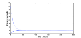
(a) $x(t)$

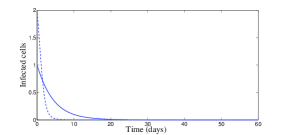
(b) $y(t)$

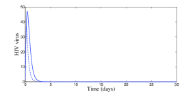
(c) $v(t)$

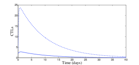
(d) $z(t)$

Figure 1: Behavior of infection for $N=750$ and parameter values (19). The continuous curves correspond to initial conditions (20) and dashed curves to initial conditions (21).

In Figure 2, we have chosen $N=1500$, which means that $\lambda\mu c-\beta aNh=7.50\times 10^{-2}>0$ and $N\beta(\lambda\mu c-\beta haN)-(\mu^{2}cd)=11.245\times 10^{-4}>0$. According to Theorem 2.4, the endemic equilibrium $E_{2}$ is locally stable. Figure 2 confirms this result numerically: we clearly see the convergence to the equilibrium point $E_{2}=(8.33,0.8,80,8.333)$. However, it is interesting to point out that, with control, a significant decrease of the infected cells, free viruses, and CTL cells, is observed (see Figure 2). The uninfected cells get maximized. It is worth to mention that with control treatment the infection dies very fast and the dynamics goes toward the disease-free equilibrium.

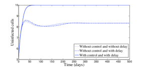
(a) $x(t)$

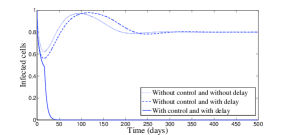
(b) $y(t)$

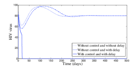
(c) $v(t)$

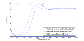
(d) $z(t)$

Figure 2: Behavior of infection during 500 days for $N=1500$, parameter values (19), and initial conditions (20): dotted line without control and without delay ($\tau=0$); dashed line without control but with delay $\tau=10$; continuous line for the delayed problem $\tau=10$ under optimal control.

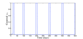
(a) $u_{1}^{*}(t)$

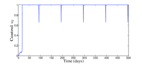
(b) $u_{2}^{*}(t)$

Figure 3: The two extremal controls $u_{1}^{*}$ and $u_{2}^{*}$ for the delayed optimal control problem (17) with $N=1500$, parameter values (19), and initial conditions (20), obtained using Algorithm 1.

The behavior of the two treatments during time is given in Figure 3. We can see that the first control makes several switchings from zero to one and vice versa. We can understand from this that one can manage the first treatment to the patient periodically in full manner. In this figure, we can also see that the second control is almost equal to one but with sudden decreases, for some short periods of time, without vanishing.

5 Conclusion

In this work we have studied a delayed HIV viral infection model with CTL immune response. The considered model includes four differential equations describing the interaction between the uninfected cells, infected cells, HIV free viruses and CTL immune response. An intracellular time delay and two treatments are incorporated to the suggested model. First, existence, positivity and boundedness of solutions are established. Next, an optimization problem is formulated in order to search the better optimal control pair to maximize the number of uninfected cells, reduce the infected cells and minimize the viral load. Two control functions are incorporated in the model, which represent the efficiency of drug treatment in inhibiting viral production and preventing new infections. The existence of such optimal control pair is established and the optimality system is given and solved numerically, using a forward and backward difference approximation scheme. It was shown that the obtained optimal control pair increases considerably the number of CD4+ cells while reducing the number of infected. Moreover, it was also observed that, under optimal control, the viral load decreases significantly compared with the model without control, which will improve the life quality of the patient. It remains an open question how to prove stability of the endemic equilibrium $E_{2}$ of model (2) for an arbitrary intracellular time delay $\tau>0$.

References

• (1) Blattner, W., Gallo, R. C., Temin, H. M.: HIV causes AIDS, Science 241(4865), 515–516 (1988)
• (2) Busch, M. P., Satten, G. A.: Time course of viremia and antibody seroconversion following human immunodeficiency virus exposure, Amer. J. Med. 102(5B), 117–126 (1997)
• (3) Ciupe, M. S., Bivort, B. L., Bortz, D. M., Nelson, P. W.: Estimating kinetic parameters from HIV primary infection data through the eyes of three different mathematical models, Math. Biosci. 200(1), 1–27 (2006)
• (4) Culshaw, R., Ruan, S., Spiteri, R. J.: Optimal HIV treatment by maximising immune response, J. Math. Biol. 48(5), 545–562 (2004)
• (5) De Boer, R. J., Perelson, A. S.: Target cell limited and immune control models of HIV infection: a comparison, J. Theor. Biol. 190(3), 201–214 (1998)
• (6) Denysiuk, R., Silva, C. J., Torres, D. F. M.: Multiobjective optimization to a TB-HIV/AIDS coinfection optimal control problem, Computational and Applied Mathematics, in press. DOI: 10.1007/s40314-017-0438-9 arXiv:1703.05458
• (7) Fleming, W. H., Rishel, R. W.: Deterministic and stochastic optimal control, Springer, Berlin (1975)
• (8) Göllmann, L., Kern, D., Maurer, H.: Optimal control problems with delays in state and control variables subject to mixed control-state constraints, Optimal Control Appl. Methods 30(4), 341–365 (2009)
• (9) Hale, J. K., Verduyn Lunel, S. M.: Introduction to functional-differential equations, Applied Mathematical Sciences, 99, Springer, New York (1993)
• (10) Kahn, J. O., Walker, B. D.: Acute human immunodeficiency virus type 1 infection, New Engl. J. Med. 339(1), 33–39 (1998)
• (11) Kirschner, D.: Using mathematics to understand HIV immune dynamics, Notices Amer. Math. Soc. 43(2), 191–202 (1996)
• (12) Lukes, D. L.: Differential equations, Mathematics in Science and Engineering, 162, Academic Press, London (1982)
• (13) Nowak, M., May, R.: Mathematical biology of HIV infection: antigenic variation and diversity threshold, Math. Biosci. 106(1), 1–21 (1991)
• (14) Pawelek, K. A., Liu, S., Pahlevani, F., Rong, L.: A model of HIV-1 infection with two time delays: mathematical analysis and comparison with patient data, Math. Biosci. 235(1), 98–109 (2012)
• (15) Perelson, A. S., Nelson, P. W.: Mathematical analysis of HIV-1 dynamics in vivo, SIAM Rev. 41(1), 3–44 (1999)
• (16) Perelson, A. S., Neumann, A. U., Markowitz, M., Leonard, J. M., Ho, D. D.: HIV-1 dynamics in vivo: virion clearance rate, infected cell life-span, and viral generation time, Science 271(5255), 1582–1586 (1996)
• (17) Rocha, D., Silva, C. J., Torres, D. F. M.: Stability and optimal control of a delayed HIV model, Math. Methods Appl. Sci., in press. DOI: 10.1002/mma.4207 arXiv:1609.07654
• (18) Silva, C. J., Torres, D. F. M.: Modeling TB-HIV syndemic and treatment, J. Appl. Math. 2014, Art. ID 248407, 14 pp (2014) arXiv:1406.0877
• (19) Silva, C. J., Torres, D. F. M.: A TB-HIV/AIDS coinfection model and optimal control treatment, Discrete Contin. Dyn. Syst. 35(9), 4639–4663 (2015) arXiv:1501.03322
• (20) Silva, C. J., Torres, D. F. M.: A SICA compartmental model in epidemiology with application to HIV/AIDS in Cape Verde, Ecological Complexity 30, 70–75 (2017) arXiv:1612.00732
• (21) Silva, C. J., Torres, D. F. M.: Modeling and optimal control of HIV/AIDS prevention through PrEP, Discrete Contin. Dyn. Syst. Ser. S 11(1), 119–141 (2018) arXiv:1703.06446
• (22) Stafford, M. A., Corey, L., Cao, Y., Daar, E. S., Ho, D. D., Perelson, A. S.: Modeling plasma virus concentration during primary HIV infection, J. Theor. Biol. 203(3), 285–301 (2000)
• (23) Wang, Y., Zhou, Y., Brauer, F., Heffernan, J. M.: Viral dynamics model with CTL immune response incorporating antiretroviral therapy, J. Math. Biol. 67(4), 901–934 (2013)
• (24) Weiss, R.: How does HIV cause AIDS?, Science 260(5112), 1273–1279 (1993)