Local Visual Microphones: Improved Sound Extraction from Silent Video

Abstract

Sound waves cause small vibrations in nearby objects. A few techniques exist in the literature that can extract sound from video. In this paper we study local vibration patterns at different image locations. We show that different locations in the image vibrate differently. We carefully aggregate local vibrations and produce a sound quality that improves state-of-the-art. We show that local vibrations could have a time delay because sound waves take time to travel through the air. We use this phenomenon to estimate sound direction. We also present a novel algorithm that speeds up sound extraction by two to three orders of magnitude and reaches real-time performance in a 20KHz video.

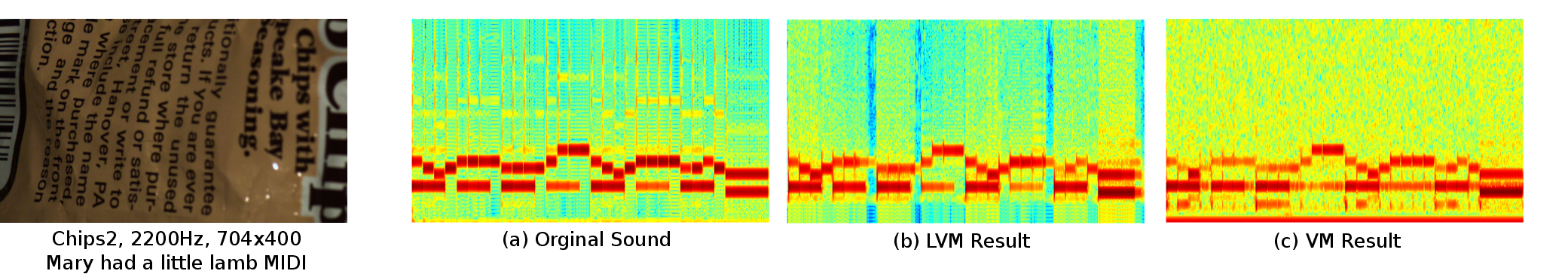
Figure 1: Left: Input high-speed video, a: Spectrogram of original sound. b: Spectrogram of our recovered sound. c: Spectrogram of sound recovery by [Davis et al.(2014)Davis, Rubinstein, Wadhwa, Mysore, Durand, and Freeman].

1 Introduction

Sound is a wave of pressure and displacement through air or a different medium. When sound waves hit an object, they cause tiny vibrations on the objects. These vibrations are sometimes detectable. Sound extraction techniques [Wang et al.(2014)Wang, Nguyen, and Quisberth, Davis et al.(2014)Davis, Rubinstein, Wadhwa, Mysore, Durand, and Freeman, Zalevsky et al.(2009)Zalevsky, Beiderman, Margalit, Gingold, Teicher, Mico, and Garcia] work by measuring tiny displacements over time in a high-speed video. Displacements as low as one hundredth of a pixel can be detected in good conditions [Guizar-Sicairos et al.(2008)Guizar-Sicairos, Thurman, and Fienup, Zhang et al.(2016)Zhang, Guo, Lei, and Zhu, Foroosh et al.(2002)Foroosh, Zerubia, and Berthod].

Sound extraction techniques prior to this work either measure global image displacement [Zhang et al.(2016)Zhang, Guo, Lei, and Zhu, Wang et al.(2014)Wang, Nguyen, and Quisberth] or measure local displacements and compute a weighted average according to the richness of texture [Davis et al.(2014)Davis, Rubinstein, Wadhwa, Mysore, Durand, and Freeman]. A texture-rich area in the image does not necessarily detect a stronger sound signal because multiple other factors affect signal quality.

Different areas in a scene react differently to incoming sound. In fact, the way an object reacts to sound strongly depends on a number of factors: material, object geometry, sound frequency and distance. Also, the way vibrations are visible to camera depends on a few other factors: texture, direction with respect to image plane, and edge direction. We study these effects in Section 4 .

Due to the above factors different areas of the image will have vibrations with different amplitudes, phases and frequency characteristics. As a result, simply averaging local vibrations will distort sound quality. One of the contributions of this paper is to examine vibrations in local areas and generate global sound by carefully aggregating vibrations in local areas. As a result, We improve the state-of-the-art of sound extraction quality. As a byproduct of our local vibration analysis, we can extract further information from silent video including the direction of the incoming sound.

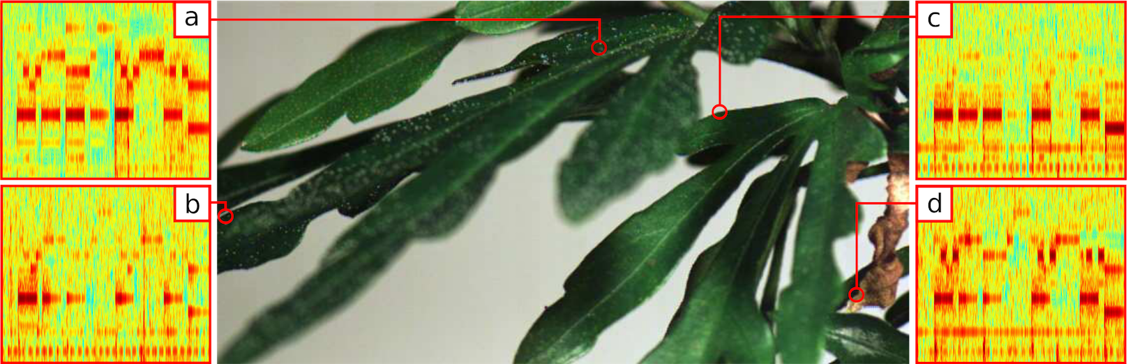
Figure 2: Different locations in the image vibrate differently and capture different aspects of the sound. Each one of the four spectrograms is from a different location. Please note that these four locations have different sound qualities and frequency characteristics.

Our experiments show that a there is a small subset of all pixels that carry most of the sound information. Most pixels carry little sound information. Another benefit of local sound extraction is that we can aggressively cut down computation cost by limiting computation to only the most useful pixels (processing high speed video is computationally intensive).

We developed a very fast algorithm to extract sound. Our algorithm performs less than 20 arithmetic operations per every pixel that is processed. As a result, our vibration detection algorithm has a throughput of about 1 Gigapixels per second on a commodity computer. As a result, our algorithm runs in real-time on a 20KHz video.

2 Prior Work

Motion extraction from a video has a wide range of applications. In the 1980s, the first applications of motion extraction were in biomedical imaging [Althof et al.(1997)Althof, Wind, and Dobbins, Alves and Tavares(2015)] and video compression [Sullivan and Baker(1991)]. Today, motion extraction has more diverse applications. In health, Zeev et al [Zalevsky et al.(2009)Zalevsky, Beiderman, Margalit, Gingold, Teicher, Mico, and Garcia] extracted heartbeats by detecting tiny movements using an optical interferometer. Balakrishnan et al [Balakrishnan et al.(2013)Balakrishnan, Durand, and Guttag], attempted to detect heart rate by tracking a number of key-points on a patient’s head.

In civil engineering, Young-Jin et al [Cha et al.(2015)Cha, Chen, and Buyukozturk] used motion magnification to detect structural damages in urban structures. In physics, Xue et al [Xue et al.(2014)Xue, Rubinstein, Wadhwa, Levin, Durand, and Freeman] used motion detection to estimate the speed of moving hot air or similar transparent fluids against a textured background. In material engineering, Davis et al [Davis et al.(2015)Davis, Bouman, Chen, Rubinstein, Durand, and Freeman] used sub-pixel motion extraction to estimate certain material properties from a video [Davis et al.(2015)Davis, Bouman, Chen, Rubinstein, Durand, and Freeman]. In 3D video processing, motion detection is used to extract depth map from binocular images [Ideses et al.(2007)Ideses, Yaroslavsky, and Fishbain, Chang et al.(2007)Chang, Fang, Ding, Chen, and Chen].

For sound detection, Zeev et al [Zalevsky et al.(2009)Zalevsky, Beiderman, Margalit, Gingold, Teicher, Mico, and Garcia] extracted speech signals by measuring the vibration of people’s neck in a video. Davis et al [Davis et al.(2014)Davis, Rubinstein, Wadhwa, Mysore, Durand, and Freeman] used sub-pixel motion extraction to recover sound from silent video. They extract vibration separately in a number of scales and angles. Then they align signals temporally (to avoid destructive interference) and finally they take a weighted average among all orientations and scales.

Before we go over further details of prior work, we need to establish relevant notations and assumptions. We assume we are given an input video $F$, that refers to a sequence of $l$ frames $F_{1}\ldots F_{l}$. For simplicity, we assume video frames are 1-D gray-scale vectors as opposed to 2-D color matrices. We assume each frame $F_{t}$ ($1\leq t\leq l$) is a vector of length $m$. Here, $F_{t}(x)$ refers to the intensity of the $x$’th pixel in the $t$’th frame ($x,t\in\mathbb{N}$). Figure 4 illustrates our notation in more details.

In order to extract motion, we need to compute displacement over time. We measure displacement with respect to a reference frame $F_{r}$. We define displacement in $F_{t}$ as $d_{r}(t)$ (where $r$ identifies reference frame) or simply $d(t)$. A simple way to measure $d(t)$ is to use cross-correlation:

$$d_{r}(t)=\operatorname*{arg\,max}_{\Delta x}\sum_{x}F_{r}(x)F_{t}(x-\Delta x)$$ (1)

Basic cross-correlation gives a precision of one pixel. In applications where displacement is significantly larger than one pixel, variants of cross-correlation [Anandan(1989), Barman et al.(1991)Barman, Haglund, Knutsson, and Granlund, Kalivas and Sawchuk(1991)] or feature point tracking [Liu et al.(2005)Liu, Torralba, Freeman, Durand, and Adelson, Zalevsky et al.(2009)Zalevsky, Beiderman, Margalit, Gingold, Teicher, Mico, and Garcia] often produce satisfactory precision. However, in cases where displacement is less than one pixel, sub-pixel precision algorithms are needed.

A number of approaches to compute sub-pixel displacement have been proposed. These approaches generally interpolate cross-correlation to sub-pixel precision and calculate $\Delta x$ in sub-pixel precision [Tian and Huhns(1986), Guizar-Sicairos et al.(2008)Guizar-Sicairos, Thurman, and Fienup, Zhang et al.(2016)Zhang, Guo, Lei, and Zhu].

Guizar-Sicairos et al [Guizar-Sicairos et al.(2008)Guizar-Sicairos, Thurman, and Fienup] first compute displacement with a precision of one pixel using cross-correlation. Then, they further refine displacement using interpolation. After finding motion in pixel precision, Zhang et al [Zhang et al.(2016)Zhang, Guo, Lei, and Zhu] proposed two different methods to refine $d(t)$. They use Taylor approximation to interpolate cross-correlation to sub-pixel precision.

Another approach is to apply a bandpass filter on a sequence of pixel intensities and extract frequency bands of interest [Wu et al.(2012)Wu, Rubinstein, Shih, Guttag, Durand, and Freeman, Wadhwa et al.(2013)Wadhwa, Rubinstein, Durand, and Freeman, Elgharib et al.(2015)Elgharib, Hefeeda, Durand, and Freeman, Foroosh et al.(2002)Foroosh, Zerubia, and Berthod]. Wadhwa et al [Wadhwa et al.(2013)Wadhwa, Rubinstein, Durand, and Freeman] first decompose images into different spatial scales and orientations. Then, they use complex-steerable-pyramids to separate the amplitude of local wavelets. Finally, they apply a temporal filter on phases at each location, orientation, and scale.

3 Motion Extraction Algorithm

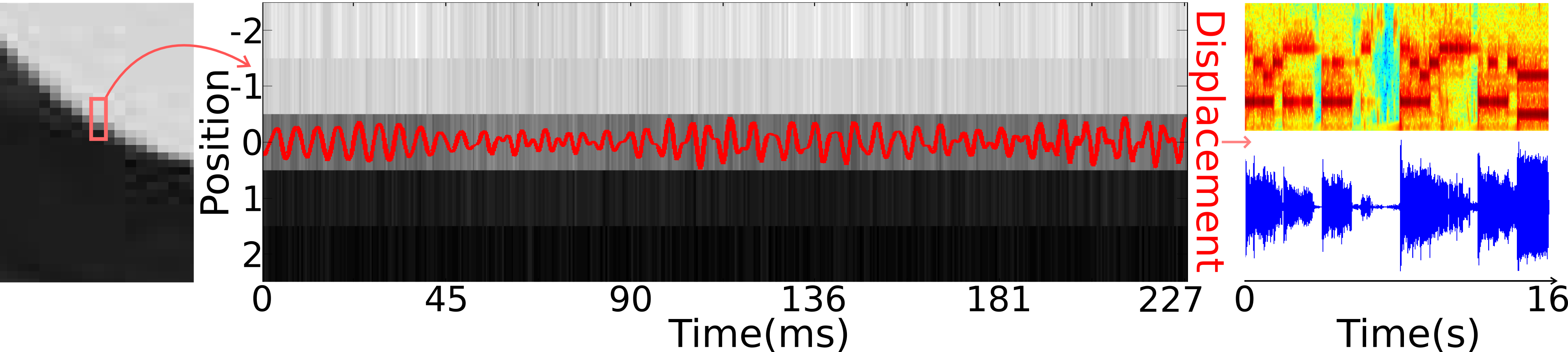
Figure 3: An illustration of sound extraction process. Left: a $5\times 1$ pixels location in the image. Middle: the value of these five pixels over a fraction of a second. In this figure pixel intensity variations are exaggerated five times and displacement (red curve) is exaggerated 50 times. Right: Extracted sound from video. Note that vibration amplitude could be as small as one-hundredth of a pixel. We capture this tiny displacement at several locations to extract sound.

Given $F_{r}$, $F_{t}$, and $\Delta x$, we define operator $K$ as follows:

$$K(F_{r},F_{t},\Delta x)=\sum_{x}F_{r}(x)F_{t}(x-\Delta x)~{}~{}~{}~{}~{}~{}~{}\forall\Delta x\in\mathbb{Z}.$$ (2)

Operator $K$ displaces $F_{t}$ by $\Delta x$ and then computes its similarity with $F_{r}$. As noted in Equation 1, to find the displacement between $F_{t}$ and $F_{r}$, we find a displacement $\Delta x$ that maximizes $K(F_{r},F_{t},\Delta x)$.

$$\operatorname*{arg\,max}_{\Delta x}K(F_{r},F_{t},\Delta x);$$ (3)

For $\Delta x\in\mathbb{Z}$ calculations of Equations 2 and 3 are straightforward. To extend $K(F_{r},F_{t},\Delta x)$ for real values of $\Delta x$ we can interpolate this function (other alternatives to interpolation were discussed in Section 2). To compute displacement with sub-pixel precision, we first estimate the integer part of displacement using Equation 3, and then estimate sub-pixel fraction using interpolation.

We evaluate $K(F_{r},F_{t},\Delta X)$ for $\Delta x\in\{-1,0,1\}$ and define $\hat{K}$ for real values of $-1\leq\Delta x\leq 1$ as a quadratic function:

$$\hat{K}(F_{r},F_{t},\Delta x)~{}=~{}a{\Delta x}^{2}~{}+~{}b\Delta x~{}+~{}c~{}~{}~{}~{}~{}~{}~{}~{}~{}~{}~{}\forall\Delta x\in\mathbb{R},-1\leq\Delta x\leq 1$$ (4)

To estimate sub-pixel displacement, we estimate $a,b,c$ and choose a $\Delta x$ that maximizes $\hat{K}$. Figure 4 illustrates this process in more details.

Function $\operatorname*{arg\,max}_{\Delta x}K(F_{r},F_{i},\Delta x)$

       $f(0)=K(F_{r},F_{i},0);$

       $f(1)=K(F_{r},F_{i},1);$

       $f(-1)=K(F_{r},F_{i},-1);$

       $d=\dfrac{f(-1)-f(1)}{2f(1)+2f(-1)-4f(0)};$

       return d;

      

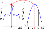
Figure 4: Left: Simple pseudo-code to estimate displacement according to similarity function $K(F_{r},F_{i},\Delta x)$. Right: An illustration of cross-correlation around $\Delta x=0$ and how we estimate displacement using a quadratic interpolation.

3.1 Further Considerations in Motion Extraction

Measure of Similarity: For image-registration and template-matching, often cross-correlation is normalized to remove the effects of magnitude of intensity, Equation 5.

$$\bar{K}(F_{r},F_{t},\Delta x)={{{\sum}}_{x}\frac{F_{r}(x)F_{t}(x-\Delta x)}{\sigma_{r}\sigma_{t}}}$$ (5)

Quartic Interpolation: We can use a quartic interpolation as opposed to quadratic interpolation. For quartic interpolation we use five points instead of 3 points. In Section 7, we compare the two techniques.

Tracking: We discussed computation of displacement for the case $|\Delta x|<1$. In cases where $|\Delta x|>1$, we need to first approximate the integer part of displacement. In a high-speed camera, displacement between two pixels is very small. In our case it is less than a hundredth of a pixel most of the time. Therefore, we track displacement and reuse its integer part. In fact the integer part of displacement can move by at most one pixel between two consecutive frames.

Two dimensional: In Section 3, for simplicity, we supposed that frames are one-dimensional signals. However, We can use a two-dimensional version of $\bar{K}$ and estimate both vertical and horizontal displacements at once.

Global vs. Local: As $\Delta x$ varies in different parts of the image, instead of calculating a global displacement signal, we partition the image into several blocks and compute displacement in each block separately. We discuss this in more details in Section 4.

4 Local Sound Extraction

When a sound is played in a scene, different areas in the scene react differently to the incoming sound, Figure 2. In fact, a number of factors affect how a certain point on an object vibrates given an incoming sound:

• Material: Some materials react more strongly to incoming sound than other materials. Generally, in higher sound frequencies, thinner and lighter objects vibrate more strongly than thicker objects [Davis et al.(2014)Davis, Rubinstein, Wadhwa, Mysore, Durand, and Freeman].

• Geometry: In one-dimensional objects (such as a rope or a rod) anti-nodes vibrate more than nodes. Vibration response from two-dimensional objects is more complex.

• Frequency: Objects respond to different frequencies differently. Resonance frequencies amplify vibration while other frequencies lead to phase shift.

• Distance: In a 20KHz video, sound waves move about 17 millimeters between every two frames. Therefore, objects that are farther to the sound source will experience some delay. Furthermore, a point that is twice farther to the sound source receives one-fourth of power and half of vibration amplitude.

All of the above factors cause some parts of the image to vibrate more or vibrate less. Further, in those parts that really vibrate, their vibration could be invisible due to a few other factors:

• Texture: Vibrations in texture-rich areas are more visible than in texture-less areas. As a result, in low-texture areas vibrations could be present but they are difficult to detect.

• Image plane: Vibrations along image plane are more visible than off-plane vibrations.

• Edge direction: Even though edges are strong textures, vibrations that are perpendicular to an edge are more visible than vibrations along an edge.

4.1 Aggregating Local Vibrations to Improve Quality

In practice, we break down the image to small blocks and then extract sound signal in each block separately. Then, we score each block by the quality of its sound signal. Most blocks have low-quality sound signals. We ignore most blocks and only keep the highest scoring ones. We use voice activity likelihood [Brookes(1997–2016)], an available software library to assign score to sound signals. We tried $8\times 8$, $16\times 16$ and $32\times 32$ blocks where $8\times 8$ produced superior results.

Due to the factors mentioned in the previous section, sound extracted from different blocks, have different amplitudes, phase-shifts and frequency characteristics (Figure 1). Due to strong phase-shifts between blocks, simple averaging of sound signals couse destructive interference and cancel out sound signal in some frequencies.

To avoid destructive interference, we combine local vibrations in a careful way. At any given frequency, each block has a different phase-shift. At each frequency, we ignore phase-shifts from all blocks and then add up the remaining signals. We perform this operation for each frequency separately and then produce an aggregate sound signal by combining all frequencies. This technique led to a state-of-the-art sound quality.

Finally, we use a noise reduction technique from [Loizou(2005)]. Our baseline [Davis et al.(2014)Davis, Rubinstein, Wadhwa, Mysore, Durand, and Freeman] reports all experimental results after the same noise reduction process. Improvements from speech enhancement is small and our technique significantly outperforms the previous state-of-the-art both before and after noise reduction.

Algorithm	Complexity
Cross Correlation	$O(n\sqrt{n})$
Up-sampled Cross Correlation	$O(nl\sqrt{nl})$
DFT registration [Guizar-Sicairos et al.(2008)Guizar-Sicairos, Thurman, and Fienup]	$O(nl\log{nl})$
Ours	$O(n)$

Table 1: Computational complexity for a number of motion extraction algorithms. Our algorithm has linear complexity with respect to the number of pixels that are processed.

Figure 5: Sound quality in several image blocks. Brighter patches are estimated to have higher sound quality. Please note that edges capture vibration more strongly.

5 Real-time performance

Not only does our algorithm beat state-of-the-art sound quality, it is also orders of magnitude faster than previous algorithms. Our algorithm runs in real time and we can cite three reasons for this speed-up.

• Fast registration algorithms: Given an $m\times m$ image with $n=m\times m$ pixels, all previous algorithms have super-linear complexities. However, since we track the integer part of displacement and compute similarity function $K$ only three times for each block, our algorithm has a complexity of $O(n)$, Table 1. In fact our algorithm uses less than 20 floating-point operations per pixel. As a result, our computation complexity is linear and memory bound.

• Pruning low-quality locations: Our experiments show that most of sound signal is concentrated in a few small neighborhoods (Figure 7). We use techniques to perform computation on only local blocks that are expected to produce high quality sound.

• Hardware optimization: We use multi-threading, CPU intrinsics and careful cache handling techniques to speed up computation. Unlike complex algorithms like DFT we don’t need floating-point arithmetic. Our core computation runs with 16-bit fixed point operations. As a result, we can perform 16 arithmetic operations in each AVX instruction.

5.1 Sound Extraction with a Few Pixels

We can prune low-quality pixels in the image more aggressively. We noticed that the intensity of a single pixel over time produces a comprehensible sound. Moreover, taking a weighted average over the intensities of a number of top-rated pixels, gives a moderate sound quality. In Section 7, we evaluate the performance of this technique. We assign weights to pixels using voice activation likelihood [Brookes(1997–2016)]. Figure 7 shows an image with a number of top-ranking pixels. We compute the mask at first by using a small segment of the video and use it for the rest of the video.

6 Sound Directions

Sound waves travel at a speed of about 340 m/s in air. In a 20KHz video, sound waves travel about 17 millimeters between every two frames. These shifts help us estimate a few factors including sound orientation. To do so, we first extract sound from all blocks and choose high quality ones. Then, we specify one block as $t_{0}$ and compute time shift for other blocks using cross-correlation. We finally regress a direction vector that shows sound direction. We applied this technique on a few different time intervals and frequencies and they agreed. Figure 7 illustrates time delays and sound direction.

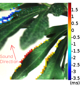
Figure 6: Some blocks receive incoming sound slightly earlier than some others. This figure identifies time-shifts for different blocks. We estimate sound direction according to time-shifts.

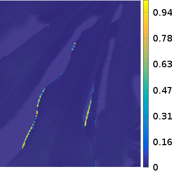
Figure 7: Not all pixels have equal sound quality. This figure visualizes sound quality at various pixels.

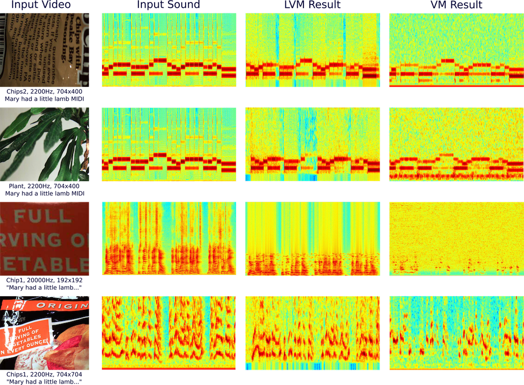
Figure 8: Input Video: In the first two videos a melody is played while in the last two videos a human voice is played. Input Sound: Spectrogram of input sound that is played in the video. LVM Result: Spectrogram of our captured sound. VM Result: Spectrogram of sound extracted by [Davis et al.(2014)Davis, Rubinstein, Wadhwa, Mysore, Durand, and Freeman].

7 Experimental Results

7.1 Sound Extraction

Davis et al [Davis et al.(2014)Davis, Rubinstein, Wadhwa, Mysore, Durand, and Freeman] established a benchmark with four high-speed videos. These videos are captured at 2KHz to 22KHz frame-rates. Two videos were captured during a melody playback. Two videos were captured during a speech playback. All videos are silent and the goal is to recover sound from silent high-speed videos. We compare our technique to Davis et al [Davis et al.(2014)Davis, Rubinstein, Wadhwa, Mysore, Durand, and Freeman] on all four videos. Figure 8 illustrates the four videos along with the spectrograms of their recovered sound. This figure compares our technique with the previous baseline.

We quantify sound quality using three measures: Perceptual Evaluation of Speech Quality (Table 2), Log-likelihood ratio (Table 3), and Segmental SNR (Table 4). We use Segmental SNR and Mean LLR for all four videos. We used Perceptual Evaluation of Speech Quality (PESQ) only for the two human speech videos (PESQ is only designed for speech). We chose these methods because they are invariant to small time-shifts.

Tables 2, 3 and 4, also compare our technique using both quartic interpolation with quadratic interpolation. Quartic interpolation leads to better sound quality, however, it comes at about twice computational cost. These tables, also compare the quality of sound extraction using only a single pixel (the best pixel). The quality of a single pixel is not as good as the rest of techniques, however, it is noteworthy that a single pixel can produce comprehensible sound.

PESQ Score	Global Sound Extraction	Single Pixel Mask	VM [Davis et al.(2014)Davis, Rubinstein, Wadhwa, Mysore, Durand, and Freeman]	Quadratic LVM(ours)	Quartic LVM(ours)
Chips1, 2200Hz	1.168	2.385	2.486	2.708	3.047
Chips1, 20000Hz	0.408	1.032	1.280	1.878	2.174

Table 2: PESQ measurements for recovered sounds. PESQ score ranges between $[0,5]$ and higher scores indicate higher quality.

MeanLLR	Global Sound Extraction	Single Pixel Mask	VM [Davis et al.(2014)Davis, Rubinstein, Wadhwa, Mysore, Durand, and Freeman]	Quadratic LVM(ours)	Quartic LVM(ours)
Chips1-2200Hz	1.394	1.453	1.019	1.027	1.021
Chips1-20000Hz	1.272	1.250	3.566	1.233	1.277
Chips2-2200Hz	0.847	1.242	0.591	0.522	0.407
Plant-2200Hz	1.027	1.190	0.853	0.572	0.510

Table 3: Log-likelihood ratio measurements for recovered sounds. Lower Log-likelihood ratios indicate higher quality. As shown in the table, quartic and quadratic interpolation can lead to the lowest Log-likelihood ratio.

SegSNR	Global Sound Extraction	Single Pixel Mask	VM [Davis et al.(2014)Davis, Rubinstein, Wadhwa, Mysore, Durand, and Freeman]	Quadratic LVM(ours)	Quartic LVM(ours)
Chips1-2200Hz	-1.3426	0.0764	1.2255	1.2621	1.276
Chips1-20000Hz	-2.4603	-1.1529	-2.2569	-1.0065	-0.837
Chips2-2200Hz	-0.0206	-4.9062	1.6254	1.7942	2.7688
Plant-2200Hz	1.0115	0.2378	2.7778	3.6434	4.5339

Table 4: Comparison of sound extraction techniques using segmental signal to noise ratios (Segmental SNR). a higher segmental SNR scores indicate higher quality. Our technique outperforms the baseline according to Segmental SNR, Log-likelihood ratio and PESQ measures.

7.2 Estimation Of Material Properties

Vibration analysis can help determine certain material properties including Young’s modulus. We compare our results on this task with that of [Davis et al.(2015)Davis, Bouman, Chen, Rubinstein, Durand, and Freeman]. This experiment includes high-speed videos of clamped rods with different materials in two lengths, once clamped to a length of 15 inches and once clamped to a length of 22 inches. There is a connection between a material’s Young’s modulus and fundamental frequency (first mode) [Shabana(1991)]. Figure 9 shows estimated frequency modes of an aluminum rod clamped to a length of 22 inch. Table 5 compares our results.

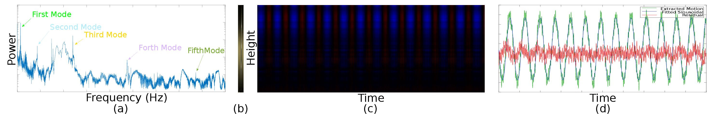
Figure 9: (a) Vibration of an aluminum rod in frequency domain. Each spike marks a candidate frequency mode. (b) A frame from video of this aluminum rod. (c) Estimated displacement over time at different times. Displacement to the left and right are marked by red and blue. (d) The first mode of vibration and the residual.

$\%$ Error	Aluminum	Brass	Copper	Steel
$22$ in - Ours	-8.23	-0.31	-1.31	-10.01
$22$ in - Visual Vibrometry	-8.94	-0.95	-1.49	-10.97
$15$ in - Ours	-14.07	-6.12	-4.21	-15.17
$15$ in - Visual Vibrometry	-22.59	-6.39	-5.01	-15.09

Table 5: Comparison of methods according to Young’s modulus estimation error.

8 Discussion

We developed a fast algorithm to extract sound from high-speed videos. We showed that different parts of image vibrate differently and we can improve sound quality by carefully combining local vibrations. Our algorithm has state-of-the-art performance both in terms of sound quality and speed. We also extract further information from videos such as sound direction.

There are a number of possible direction for future work. In theory, if there are multiple sources of sound, it could be possible to separate sounds from different sources. Real-time processing of small motions could have several practical applications in Medical Science, and Engineering. Also our regular memory access pattern opens the possibility to benefit from further hardware accelerators including GPU.

9 Acknowledgements

We greatly thank Dr. Mostafa Kamali Tabrizi, Dr. S. Ebadolah Mahmoudian and Dr. Mohammad Reza Razvan for their support and their valuable comments. This work was partially supported by National Elites Foundation of Iran.

References

- [Althof et al.(1997)Althof, Wind, and Dobbins] Raymond J Althof, Marco GJ Wind, and James T Dobbins. A rapid and automatic image registration algorithm with subpixel accuracy. IEEE transactions on medical imaging, 16(3):308–316, 1997.
- [Alves and Tavares(2015)] Raquel S Alves and João Manuel RS Tavares. Computer image registration techniques applied to nuclear medicine images. In Computational and Experimental Biomedical Sciences: Methods and Applications, pages 173–191. Springer, 2015.
- [Anandan(1989)] Padmanabhan Anandan. A computational framework and an algorithm for the measurement of visual motion. International Journal of Computer Vision, 2(3):283–310, 1989.
- [Balakrishnan et al.(2013)Balakrishnan, Durand, and Guttag] G. Balakrishnan, F. Durand, and J. Guttag. Detecting pulse from head motions in video. In Computer Vision and Pattern Recognition (CVPR), 2013 IEEE Conference on, pages 3430–3437, June 2013. 10.1109/CVPR.2013.440.
- [Barman et al.(1991)Barman, Haglund, Knutsson, and Granlund] H. Barman, L. Haglund, H. Knutsson, and G. H. Granlund. Estimation of velocity, acceleration and disparity in time sequences. In Visual Motion, 1991., Proceedings of the IEEE Workshop on, pages 44–51, Oct 1991. 10.1109/WVM.1991.212789.
- [Brookes(1997–2016)] Mike Brookes. VOICEBOX: A speech processing toolbox for MATLAB. Software library, Imperial College London, 1997–2016. URL http://www.ee.imperial.ac.uk/hp/staff/dmb/voicebox/voicebox.html.
- [Cha et al.(2015)Cha, Chen, and Buyukozturk] Young-Jin Cha, Justin G Chen, and Oral Buyukozturk. Motion magnification based damage detection using high speed video. In Proceedings of the 10th International Workshop on Structural Health Monitoring (IWSHM), Palo Alto, CA, USA, pages 1–3, 2015.
- [Chang et al.(2007)Chang, Fang, Ding, Chen, and Chen] Yu-Lin Chang, Chih-Ying Fang, Li-Fu Ding, Shao-Yi Chen, and Liang-Gee Chen. Depth map generation for 2d-to-3d conversion by short-term motion assisted color segmentation. In 2007 IEEE international conference on multimedia and expo, pages 1958–1961. IEEE, 2007.
- [Davis et al.(2015)Davis, Bouman, Chen, Rubinstein, Durand, and Freeman] A. Davis, K. L. Bouman, J. G. Chen, M. Rubinstein, F. Durand, and W. T. Freeman. Visual vibrometry: Estimating material properties from small motions in video. In 2015 IEEE Conference on Computer Vision and Pattern Recognition (CVPR), pages 5335–5343, June 2015. 10.1109/CVPR.2015.7299171.
- [Davis et al.(2014)Davis, Rubinstein, Wadhwa, Mysore, Durand, and Freeman] Abe Davis, Michael Rubinstein, Neal Wadhwa, Gautham Mysore, Fredo Durand, and William T. Freeman. The visual microphone: Passive recovery of sound from video. ACM Transactions on Graphics (Proc. SIGGRAPH), 33(4):79:1–79:10, 2014.
- [Elgharib et al.(2015)Elgharib, Hefeeda, Durand, and Freeman] Mohamed A. Elgharib, Mohamed Hefeeda, Frédo Durand, and William T. Freeman. Video magnification in presence of large motions. In CVPR, 2015.
- [Foroosh et al.(2002)Foroosh, Zerubia, and Berthod] Hassan Foroosh, Josiane B Zerubia, and Marc Berthod. Extension of phase correlation to subpixel registration. IEEE transactions on image processing, 11(3):188–200, 2002.
- [Guizar-Sicairos et al.(2008)Guizar-Sicairos, Thurman, and Fienup] Manuel Guizar-Sicairos, Samuel T. Thurman, and James R. Fienup. Efficient subpixel image registration algorithms. Opt. Lett., 33(2):156–158, Jan 2008. 10.1364/OL.33.000156. URL http://ol.osa.org/abstract.cfm?URI=ol-33-2-156.
- [Ideses et al.(2007)Ideses, Yaroslavsky, and Fishbain] Ianir Ideses, Leonid P Yaroslavsky, and Barak Fishbain. Real-time 2d to 3d video conversion. Journal of Real-Time Image Processing, 2(1):3–9, 2007.
- [Kalivas and Sawchuk(1991)] Dimitrios S Kalivas and Alexander A Sawchuk. A region matching motion estimation algorithm. CVGIP: Image Understanding, 54(2):275–288, 1991.
- [Liu et al.(2005)Liu, Torralba, Freeman, Durand, and Adelson] Ce Liu, Antonio Torralba, William T. Freeman, Frédo Durand, and Edward H. Adelson. Motion magnification. ACM Trans. Graph., 24(3):519–526, July 2005. ISSN 0730-0301. 10.1145/1073204.1073223. URL http://doi.acm.org/10.1145/1073204.1073223.
- [Loizou(2005)] Philipos C Loizou. Speech enhancement based on perceptually motivated bayesian estimators of the magnitude spectrum. IEEE Transactions on Speech and Audio Processing, 13(5):857–869, 2005.
- [Shabana(1991)] A.A. Shabana. Theory of Vibration: Volume II: Discrete and Continuous Systems (Mechanical Engineering Series). Springer, 1991. ISBN 1468403826. URL http://www.amazon.com/Theory-Vibration-Continuous-Mechanical-Engineering/dp/1468403826%3FSubscriptionId%3D0JYN1NVW651KCA56C102%26tag%3Dtechkie-20%26linkCode%3Dxm2%26camp%3D2025%26creative%3D165953%26creativeASIN%3D1468403826.
- [Sullivan and Baker(1991)] Gary J Sullivan and Richard L Baker. Motion compensation for video compression using control grid interpolation. In Acoustics, Speech, and Signal Processing, 1991. ICASSP-91., 1991 International Conference on, pages 2713–2716. IEEE, 1991.
- [Tian and Huhns(1986)] Qi Tian and Michael N Huhns. Algorithms for subpixel registration. Computer Vision, Graphics, and Image Processing, 35(2):220–233, 1986.
- [Wadhwa et al.(2013)Wadhwa, Rubinstein, Durand, and Freeman] Neal Wadhwa, Michael Rubinstein, Frédo Durand, and William T Freeman. Phase-based video motion processing. ACM Transactions on Graphics (TOG), 32(4):80, 2013.
- [Wang et al.(2014)Wang, Nguyen, and Quisberth] Zhaoyang Wang, Hieu Nguyen, and Jason Quisberth. Audio extraction from silent high-speed video using an optical technique. Optical Engineering, 53(11):110502–110502, 2014.
- [Wu et al.(2012)Wu, Rubinstein, Shih, Guttag, Durand, and Freeman] Hao-Yu Wu, Michael Rubinstein, Eugene Shih, John V Guttag, Frédo Durand, and William T Freeman. Eulerian video magnification for revealing subtle changes in the world. 2012.
- [Xue et al.(2014)Xue, Rubinstein, Wadhwa, Levin, Durand, and Freeman] Tianfan Xue, Michael Rubinstein, Neal Wadhwa, Anat Levin, Fredo Durand, and William T. Freeman. Refraction Wiggles for Measuring Fluid Depth and Velocity from Video, pages 767–782. Springer International Publishing, Cham, 2014. ISBN 978-3-319-10578-9. 10.1007/978-3-319-10578-9_50. URL http://dx.doi.org/10.1007/978-3-319-10578-9_50.
- [Zalevsky et al.(2009)Zalevsky, Beiderman, Margalit, Gingold, Teicher, Mico, and Garcia] Zeev Zalevsky, Yevgeny Beiderman, Israel Margalit, Shimshon Gingold, Mina Teicher, Vicente Mico, and Javier Garcia. Simultaneous remote extraction of multiple speech sources and heart beats from secondary speckles pattern. Optics express, 17(24):21566–21580, 2009.
- [Zhang et al.(2016)Zhang, Guo, Lei, and Zhu] Dashan Zhang, Jie Guo, Xiujun Lei, and Changan Zhu. A high-speed vision-based sensor for dynamic vibration analysis using fast motion extraction algorithms. Sensors, 16(4):572, 2016.