Non-local elasticity theory as a continuous limit of 3D
networks of pointwise interacting masses
E. Khruslov, M. Goncharenko
Small oscillations of an elastic system of point masses
(particles) with a nonlocal interaction are considered. We study
the asymptotic behavior of the system, when number of particles
tends to infinity, and the distances between them and the forces
of interaction tends to zero. The first term of the asymptotic is
described by the homogenized system of equations, which is a
nonlocal model of oscillations of elastic medium.
Introduction
The progress in development of new materials and the modelling of
nanostructures caused the emergence of nonlinear elasticity
theories (see, for example, [1], [2], [3] ).
Classical local theory is based on the concept of contact
interaction and it can not explain some observed experimental
phenomena. Therefore, it is necessary to take into account the
long-range interaction between the particles of the material and
this leads to the nonlocal elasticity theory.
The nonlocal elasticity theory can be traced back to the works of
Kröner, who formulated the continual theory of elastic materials
with long-range interaction forces ([4], [5]). At
present, the nonlocal mechanics of the elastic continuum is
treated with two different approaches: the gradient elasticity
theory (weak nonlocality) and the integral nonlocal theory (strong
nonlocality).
The first approach is related to the study of the gradients of the
strain tensors. It leads to models with spatial derivatives of
order more than 2 ([6] - [8]). The main difficulties in
using this model are the setting of boundary conditions for the
corresponding boundary value problems (see [9]).
The second approach has been developed almost independently. The
nonlocal interaction here is represented in the form of a
convolution integral of the deformation tensor with a kernel that
depends on the distance between the particles of the elastic
material. This approach leads to models described by
integro-differential equations ([10] - [13]).
The correctness of these continuum models of nonlocal elasticity
theory depends on the effectiveness of long-range molecular forces
in the material. Therefore, a natural approach to their
justification is the so-called microstructural approach, which is
studying discrete elastic systems (lattice models). This approach
has been used mainly in physical works ([14] - [18]).
Apparently, one of the first mathematical works, in which the
system of equations of the local elasticity theory was derived
using the microstructural approach, was [19]. The short-range
interactions between particles were considered. Only the nearest
particles interact in the system. The asymptotic behavior of the
oscillations of such a system was investigated when the distances
between the nearest neighbors and the forces of interaction
between them tend to zero. A homogenized system of differential
equations describing the leading term of the asymptotic was
obtained. This system is a continuum model of the local theory of
elasticity. In this work the method based on the studying of the
asymptotic behavior of the system, when the scale of the
microstructure tends to zero, was applied. This approach is the
basis for the homogenization of partial differential equations
([20] - [22]).
We apply this approach of homogenization to study the asymptotic
behavior of the oscillations of an elastic system of point masses
(particles) with a nonlocal interaction. It is assumed that the
system depends on the small parameter . More
precisely, the distance between the nearest neighbors is of the
order , and the long-range forces are of order
. It is proved that the main term of the
asymptotic is described by a homogenized system of
integro-differential equations. The integral term is a convolution
of the difference of the displacements of the elastic medium at
various points with some kernel. Note that such a system differs
from the continual model of Eringen, where the convolution of the
deformation tensor with the kernel is taken. A similar system of
integro-differential equations was proposed earlier (without
justification) in [23] as a variant of the integral
elasticity theory and was used to calculate steel plates. The
indicated order of interactions in the system corresponds to the
integral (and not gradient) elasticity theory.
1 Statement of the problem
We consider a system of interacting point masses
(we will call them particles) in a fixed bounded domain with a smooth boundary .
It is assumed that this system depends on the small parameter
. The total number of particles in the system is
and the distances between the nearest
particles are of order . We denote by () the positions of
the particles in the equilibrium state of the system , and we denote by the displacements of particles relative to
their equilibrium positions .
The potential energy for small variation of the system
from the equilibrium position is determined by
the equality
(1.1)
where , parentheses
denote the scalar product in , and
are symmetric nonnegative matrices of the
pair interaction between the -th and -th particles. If the
particles interact through the central elastic forces (for
example, they connected by elastic springs), then the matrices
satisfy the equalities
(1.2)
where is the unit vector of
direction between the -th and -th particles and the
coefficient characterizes the intensity of
interaction (stiffness of springs).
The coefficient depends on the distances
between particles.
Generally speaking, it can be zero if the corresponding pair of
particles does not interact with each other. In this paper we
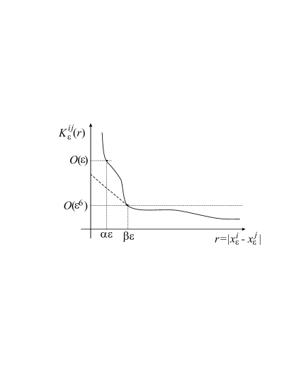
assume that the coefficient is defined by
formula
(1.3)
where , , ,
as and as ();
(for interacting pairs of particles) and
(for noninteracting pairs of particles),
.
The formula above simulates a weak interaction (of the order ) between not very close particles () and
stronger interaction between close ones
() (see Figure 1). This type of interaction is
characteristic for some intermolecular forces (for example, van
der Waals forces).
Figure 1:
The interaction energy of the system (1.1)
- (1.3) is invariant under rotations and shear. Therefore,
the equilibrium state of the system is not isolated:
rotations and shifts are allowed. To exclude this we fix the part
of the particles on the
boundary (at the corresponding points ). We
assume the following conditions hold.
I. The condition of ”-net” on the
boundary . The set of
particles assigned to is a -net
for . It is clear that the number of such
particles is
II. The triangulation condition.
Let be a graph with vertices at points and edges
(, ). Assume that for
any there exists a subgraph
with the
same set of vertices and edges of length (), that correspond to the interaction
coefficients (). The subgraph
triangulates the domain . The volumes of the corresponding simplexes of the
triangulation () satisfy the inequality ().
Under these conditions, the equilibrium state is isolated. In the small
neighborhood of the nonstationary oscillations of
the system are described by the following
problem
(1.4)
(1.5)
(1.6)
where is a mass of -th particle,
are the given initial displacements of the
particles, are the given initial velocities
(, when
). There exists a unique
solution of this problem. The main goal
of the paper is to study the asymptotic behavior of the solution
as . We obtain a homogenized system of
equations. This system describes the leading term of the
asymptotic and is a macroscopic model of the oscillation of an
elastic medium with a nonlocal interaction.
2 Quantitative characteristics of the system of interacting particles and formulation of main result
We denote by cubes with centers at points and sides of length with a fixed orientation. It
is assumed that and the cube
contains a large number of particles (of order ). Consider the following
functional of the symmetric tensor :
(2.1)
The sum consist of particles
and is taken over
displacements of these particles. The vector function is defined by equality , and is an arbitrary penalty
parameter: .
The functional is quadratic and we can rewrite it
in the form
(2.2)
where are the components of the
symmetric tensor of 4-th rank in :
. This tensor is a mesoscopic
() characteristic of the concentration of
the short-range interaction energy in a neighborhood of the point
Assume that the limits
(2.3)
exist.
Remark. Formally, the limit tensor must depend on the parameter
and the orientation of the cubes . But the main result
and the example in Section 6 show that the limiting tensor does not depend on the
parameter and the orientation of the cubes
Let be a density of
the distribution of particles masses and let be a function of the
distribution of the pairs of particles in
with long-range interaction. We will denote by
() Voronoi cells of a set of points
denotes the volume of the cell and
is a characteristic function of the cell.
Assume that
(2.4)
(2.5)
where are the masses of the particles,
are the elements of the adjacency matrix
of
the complete graph for the system
(see (1.3)).
Suppose, that for any
(2.6)
By the triangulation condition II (), and the estimates
,
are valid uniformly with respect to . Hence the set
of functions is *-weakly compact in and the set is
*-weakly compact in (see
[21], [22]).
We assume that
(2.7)
(2.8)
as . Here and
are the functions in and
respectively.
For each discrete function
that defined at the points :
we will match the
vector function by
the formula
(2.9)
The vector-functions ,
correspond to the initial data
and
in
(1.4)-(1.6). The vector-function correspond to the
solution of the
problem.
We assume that
(2.10)
as . Here and are the vector
functions from . Suppose that the
inequality
(2.11)
holds uniformly with respect to .
Now we can formulate the main result.
Theorem 2.1.
Let the system of interacting particles with the
interaction energy (1.1) - (1.3) and the masses (2.6) be located in and
conditions I and II are fulfilled. Suppose that
conditions (2.3), (2.7), (2.8) and (2.10),
(2.11) hold as . Then the vector
function constructed by
(2.9) using the solution of the problem (1.4)
- (1.6) converges in as
to the solution of the
following initial-boundary value problem
(2.12)
(2.13)
(2.14)
Here are the
components of the elasticity tensor, is the unit vector of
axis, and the elements of the matrix are defined by
The proof of the theorem is carried out in Sections 4,5. In
remainder of this Section we give the main ideas of the prove. By
the Laplace transform in time we reduce in Section 4 the initial
problem to a stationary problem with a spectral parameter (). We formulate the
variational formulation of the problem for real .
Then we study the asymptotic behavior of its solution as and obtain the homogenized equation. Using the
Vitali’s theorem we investigate in Section 5 analytic properties
of solutions of the initial and homogenized stationary problems on
for . We prove the
convergence of the solutions and, finally, we prove the
convergence of solutions of the original non-stationary problem
(1.3) - (1.6) to the solution of the homogenized
problem (2.11) - (2.13) with the help of the inverse
Laplace transform, .
3 Auxiliary propositions
Let us denote by a continuous function in
that is linear in every simplex
(condition of triangulation II) and
at
. It is clear that it is non-zero only in
simplexes with vertices .
Using this function we construct a piecewise linear spline to interpolate the given discrete
vector-function
:
(3.1)
where .
In what follows, we assume that for
. Then, for any if the domain is convex. If is not convex,
then for sufficiently small . Here is a domain in
such that and
(). This statement follows from
conditions I, II, and smoothness of the .
Lemma 3.1.
Let us construct vector-functions and
by formulas (2.9) and (3.1)
for the same set of vectors ( for
). If the inequality
holds uniformly with respect to , then
Proof. Denote by . Let be the Voronoi cell at the point , and be a simplex with
vertex at the point (see condition of
triangulation II). By (3.1) with , we get
As , the function is continuous for , and , (condition II). We
have
(3.8)
and
(3.9)
for any fixed .
From (3.5)-(3.9) follows the assertion of the lemma.
The following lemma plays a fundamental role in studying the
compactness of discrete vector-valued functions. The same role
plays the well-known Korn inequality for the functions in cite 24.
Lemma 3.3(discrete analogue of the Korn inequality).
Let conditions I and II hold.
Then
for any discrete function defined at points
by , and
for . Here
are the pair interaction matrices (see (1.1)-(1.3));
the sum is taken over all of the
edges of triangulation
subgraph , and , are the
constants that do not depend on .
4 Variational formulation of the problem and asymptotic
behavior of the solution
as
By Laplace transform we convert the function
of a real variable to the function of a complex variable
:
Applying the Laplace transform to the problem
(1.4)-(1.6) and taking into account (1.1), we
get the stationary problem for
with a spectral
parameter
(4.1)
where , .
This problem has a unique solution for all ,
except the finite number of the spectrum points (,
). For ,
the problem describes the equilibrium elastic system under the
action of the forces .
Solution of the
problem (4.1) for minimizes the functional
(4.2)
in the space of discrete
vector-functions
that equal on : when
. Thus, the vector-function
is the solution of the
minimization problem
(4.3)
To describe the asymptotic behavior of as
, we introduce in the functional
(4.4)
Here , tensor is given by (2.3), functions
and are defined by
(2.7) and (2.8), vector-function
is given by (2.10), and the
elements of the matrix are defined by (3.4).
Consider the minimization problem
(4.5)
Theorem 4.1.
Let conditions I, II, (1.2), (1.3) hold
and let the limits (2.3), (2.7), (2.8) exist as
. Then the vector-function constructed by (2.9) on the solution of the
minimization problem (4.3) converges in to the
solution of the minimization problem (4.5)
Proof. Taking into account that
and , we get the inequality
(4.6)
From (2.4), (2.7), (2.10) and condition II it
follows that
(4.7)
where does not depend on .
We construct the vector-function by
(3.1) where is the solution of (4.3) .
By inequalities (4.6), (4.7) and lemma 3.3 we get
(4.8)
The inequality is satisfied uniformly with respect to
.
Thus, the set of vector-functions is a weakly compact set in
. We can extract a subsequence
converges to
the vector-function
weakly in and strongly in
().
By (2.9) we construct the subsequence for the set of
vector-functions . According to lemma 3.1 and
(4.8) the subsequence converges to in .
Let us prove that minimizes (4.5). For this purpose
we rewrite the functional (4.2) in the
form:
(4.9)
where
(4.10)
(4.11)
Strong interactions between nearby particles are included in
functional . According to (1.2),
(1.3) this interaction has the order (see
[19]). Recalling that converges
weakly in as
, and taking into account
(2.2), we get the lower bound for by
the same method as in [19]:
(4.12)
By (1.2), (1.3), (2.4), (3.5) we can
rewrite in the form:
(4.13)
where
and is -th component of the
vector-function (2.4).
From the above, by lemma 3.2, (2.7), and (4.13), we
obtain
(4.14)
On account of (4.9), (4.13), (4.14), we get the
lower bound for :
(4.15)
where is a limit in of the vector-functions
, and the functional
is defined by (4.4).
In order to get the upper bound, we introduce the test
vector-function
in for the problem (4.3).
To this end, we cover by cubes with centers at the points and sides
of length . The centers of the cubes form a cubic lattice with
period (). By this covering we
construct the partition of unity . Namely, the
set of functions with the following properties: , ,
when , when ; .
Let be an arbitrary vector-functions in with
the compact support in . Define
(4.16)
Here is a
minimizer of the functional (2.1) in the cube
for ();
, are a symmetric and antisymmetric
parts of the tensor ; .
Using the properties of the discrete vector-functions
(see lemma 3.4), the properties of
the partition of unity , and by
(2.2) we get
(4.17)
in the same manner as in [19]. The functional is
defined by (4.12).
To estimate , we use the
following equality for the vector-functions for
Substituting this equality in (4.16) and applying lemma 3.4,
we conclude
(4.18)
Taking into account convergence (2.7), (2.10), and
lemma 3.2, we get
The inequality is valid for any vector-function
due to the continuity of the
functional in . Thus,
the limit of the vector-functions by subsequence is a solution
of minimizing problem (4.5). Consequently, is a weak
solution of the following boundary value problem
(4.21)
Since , function and matrix-function
are non-negative, and tensor
is positive definite, the problem
have a unique solution. Thus, theorem 4.1 is proved.
5 The convergence of solutions of the problem (4.1)
to the solution of the problem (4.21) for complex
1. Consider the problem (4.1) for complex in
semiaxis . Denote by a
Hilbert space of finite sets of 3-components
complex vectors defined in : . If
then .
Define a scalar product in :
where is a mass of the point .
By parenthesis we denote the scalar product
in . The bar denotes the complex conjugation. The
corresponding norm is denoted by
Consider in a linear operator :
(5.1)
From (2.5), (1.2), (1.3) it follows that
is a bounded selfadjoint operator in
. By lemma 3.3 is positive definite
operator uniformly with respect to :
(5.2)
Let us rewrite the problem (4.1) in operator form in
:
(5.3)
By the indicated properties of operator its
resolvent is a meromorphic operator function of the parameter
with poles on the negative semiaxis .
Hence the solution of
(5.3) is a holomorphic function of in the
half-plane . Multiplying (5.3) on
and separating the imaginary and real parts,
taking into account (2.5) and (2.10), we obtain the
estimate for in half-plane () uniform with respect to
:
(). This implies that the vector-function
defined by
(2.9) is a holomorphic function in (). Moreover,
is bounded in the norm of uniformly with respect to
:
(5.4)
2. We now turn to the problem (4.21). Denote by a Hilbert space of a complex-valued vector-functions in
with a weight . The scalar product in
we define by
Consider a sesquilinear form defined on the set of vector-valued
functions that is dense in
The form generates in a selfadjoint operator
, that is due to the properties of the elasticity tensor
and the long-range matrix
[21]. The equality
is valid. From the Korn’s inequality it follows that
(5.5)
This inequality implies that the operator is positive definite
and has a completely continuous inverse operator. Now we can
rewrite the problem (4.21) in operator form:
(5.6)
The properties of the operator implies that equation
(5.6) has a solution for complex
() and this solution is a holomorphic
function of satisfying the inequality
3. By theorem 2.1 the vector-function converges in for to the
solution of the problem (4.21) (or equation
(5.6)) as . Moreover, the set of
vector-functions is bounded by norm in uniformly with respect
to in the half-plane
(). Therefore, using Vitali’s theorem and taking
into account that is holomorphic, we get the
following assertion.
Theorem 5.1.
Let assumptions I, II, (2.2), (2.6),
(2.9) hold. Let construct the function by (2.9) on the solution of the problem
(4.1). Then vector-function converges in to the
solution of equation (5.6) (or the problem
(4.21)) uniformly with respect to complex from the
half-plane ().
6 The end of the proof of the main theorem
By the definition (5.1) of operator the
problem (1.4) – (1.6) is representable in
in the form:
The equality above with the discrete Korn’s inequality, the
properties of and , and
(2.9), (2.10) implies inequality:
where is a spline
vector-function, defined by (3.1), and does not depend
on .
Thus the set of vector-functions is bounded in uniformly
with respect to . We can extract a subsequence
converges
weakly in to a function (and by embedding theorem converges strongly in
() and for almost all converges strongly in ). By the above and
lemma 3.1 we conclude that the piecewise-constant vector-functions
defined by (2.9) converges in
and to for almost all as .
Let us prove that the function is a solution of the
problem (2.11) – (2.13). By definition of operator
this problem can be written in operator form:
(6.2)
The solution of the problem
(1.4)-(1.6) is an inverse Laplace transform of the
solution of the problem (4.1)
Thus we have
(6.3)
where and are defined by
(2.9). Multiply the equality above by ,
where , , and
integrate over . Changing the integration order and
integrating on by parts, we obtain
Note that the integrals on in the right-hand side
converge absolutely, due to (5.4).
Let us pass to the limit in the equation above as
. Passing to the limit we take
into account that converges to
in , and converges to the solution of the
equation (5.6) in uniformly on the compacts
from the half-plane (see theorem
2). We get
Since the linear combination of the functions
form a dense set in then is a solution of
the problem (6.2). By the properties of operator , this
problem has a unique solution. Thus converges to
in as . The theorem
1.1 is proved.
7 Periodic structure
We now consider the concrete case when the conditions of theorem
1.1 are satisfied and the elastic tensor and
the matrix-function are computed explicitly.
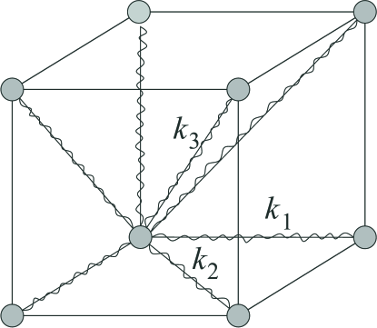
Suppose that the points of the equilibrium
state of the system are located periodically. They form a cubic
lattice with a period . Each point
interacts with the tops of the cube
. The points
belongs to the same cube. For clarity, we can assume that the
interaction is carried out by elastic springs . The stiffness of
the springs (the elasticity coefficient in Hooke’s law) directed
along the edges of the cubes is ; directed
along the diagonals of the faces of the cubes is ; and directed along the diagonals of the cubes is (Fig. 2). This is a strong short-range
interaction.
Figure 2:
The corresponding coefficients of interaction (1.2)
have an order , ,
.
Let us assume that there exist a long-range interaction. Each
point interacts with the points
of the cubic sublattice
with the period
(, ). This is a weak interaction
and
The system of the points satisfies the
triangulation condition II. The corresponding interaction is
described by (1.2), where ,
; only for and for ().
By (2.3) the limit dense is equal to
. Therefore, by (3.4)
(7.1)
The components of elasticity tensor for this system are calculated
in [19]. They are determined by formulas:
and in other cases.
Remark. If we take
, then the
components of limiting elasticity tensor are satisfying the
condition: and the limit model of
elastic system is isotropic. The equation (2.12) has a form:
where , and the elements of matrix
are defined by (7.1).
References
[1] Liew K.M., Zhang Y., Zhang L.W. Nonlocal elasticity
theory for graphene modeling and simulation: prospects and
challenges. Journal of modeling in Mechanics and Materials, 2017.
[2] Eringen A.C. Non-local polar field models. Academic
Press, New York, 1996.
[3] Gopalakrishan S., Narendar S. Wave Propagation in
Nanostructures. Nonlocal Continuum Mechanics Formulations.
Springer, 2013.
[4] Kröner E. Elasticity Theory of Materials with Long Range Cohesive Forces. Int. J. Solids and Structures, 1967, vol. 3, pp. 731-742.
[5] Kröner E. Problem of non-locality in the mechanics
of solids: review on present status. In Proceedings of the
Conference of Fundamental Aspects of Dislocation Theory.
p.729-736.
[6] Eringen, A.C. Non-local polar elastic continua. Int. J.
Eng. Sci. 10, 1972, p. 1-16.
[7] Eringen, A.C., Edelen D.G.B. On non-local elasticity. Int. J.
Eng. Sci. 10, 1972, p. 233-248.
[8] Aifantis E.C. Gradient effects at macro, micro and
nano scales. Journal of the Mechanical Behavior of Materials, 5,
1994, p. 355-375.
[9] Polizzotto C. Non local elasticity and related variational principles.
International Journal of Solids and Structure, 38, 2001,
p.7359-7380.
[10] Krumhansl, J.A., 1963. Generalized continuum field representation for lattice
vibrations. In: Wallis, R.F. (Ed.), Lattice Dynamics, Proc. of
Int. Conference. Pergamon Press, London.
[11] Kunin, I.A., 1982. Elastic Media with Microstructure I. Springer-Verlag, Berlin
[12]Di Paola, M., Failla, G., Zingales, M., 2009. Physically-based approach to the
mechanics of strong non-local elasticity theory. Journal of
Elasticity 97 (2), 103 130.
[13] Di Paola, M., Pirrotta, A., Zingales, M., 2010. Mechanically-based approach to nonlocal
elasticity: variational principles. International Journal of
Solids and Structures 47 (5), 539 548
[14] R. D. Mindlin, Theories of elastic continua and crystal lattice theories , Chapter 3, pp. 312 320 in Mechanics
of generalized continua (Stuttgart, 1967), edited by E. Kroner,
Springer, Berlin, 1968.
[15] Born M, Huang K. Dynamical Theory of Crystal Lattices. Oxford University Press: London, 1954
[16] Tarasov V. E., General lattice model of gradient elasticity, Mod. Phys. Lett. B 28:7 (2014), article 1450054
[17] Tarasov V. E., Three-dimensional lattice models with long-range interactions of Grunwald Letnikov type for
fractional generalization of gradient elasticity, Meccanica
(Milano) 51:1 (2016), 125 138.
[18] Silling S.A. Reformulation of elasticity theory for
discontinuities and long-range forces. Journal of Mechanics and
Physics of Solids, 48, 2000, p.175-209.
[19] Berezhnyy M., Berlyand L. Continium limit for three-dimensional
mass-spring network and disret Korn’s inequality. Journal of the mech. and Phys. of Solids, 54 (2006), pp. 635-669.
[20] Marchenko V.A. and Khruslov E.Ya.,
Homogenization of Partial Differential Equations.
Birkhöuser, Boston, Basel, Berlin, 2006
[21] Sanchez-Palencia E. Non-homogeneous media and
vibration theory. – Springer-Verlag Berlin Heidelberg, 1980. –
400 c.
[22] Piatnitski A.L., Chechkin G.A, Shamaev A.S.
Homogenization. Methods and applications. – Novosibirsk,
2007, 250 p.
[23] M. Di Paola, G. Failla, M. Zingales. The mechanically-based approach to 3D non-local linear elasticity theory: long-range central interactions. International Journal of Solids and Structures, 47, 2010, p. 2347-2358.
[24] Oleinik O.A., Shamaev A.S., Yosifian G.A.
Mathematical problems in elasticity and Homogenization. –
North-Holland, 1992, 250p.
[25] Markushevich A.I. The theory of analytical functions.
– Moscow: Mir Publishers, 1983, 423p.