Polaron in a non-abelian Aubry-André-Harper model with p-wave superfluidity

Abstract

We theoretically investigate the behavior of a mobile impurity immersed in a one-dimensional quasi-periodic Fermi system with topological $p$-wave superfluidity. This polaron problem is solved by using a standard variational approach, the so-called Chevy ansatz. The polaron states are found to be strongly affected by the strength of the quasi-disorder and the amplitude of the $p$-wave pairing. We analyze the phase diagram of the polaron ground state and find four phases: two extended phases, a weakly-localized phase and a strongly-localized phase. It is remarkable that these polaron phases are directly corresponding to the four distinct phases experienced by the underlying background Fermi system. In particular, the weakly-localized polaron phase corresponds to an intriguing critical phase of the Fermi system. Therefore, the different phases of the background system can be unambiguously probed by measuring the polaron properties via radio-frequency spectroscopy. We also investigate the high-lying excited polaron states at an infinite temperature and address the possibility of studying many-body localization (MBL) of these states. We find that the introduction of $p$-wave pairing may delocalize the many-body localized states and make the system easier to thermalize. Our results could be observed in current state-of-the-art cold-atom experiments.

I Introduction

Impurity and disorder are key ingredients of many intriguing phenomena in quantum systems. Disorder in a non-interacting system can lead to an unexpected phenomenon, namely Anderson localization (AL) PWAnderson1958 , which has been widely investigated and observed experimentally in various systems, including microwaves RDalichaouch1991 ; AAChabanov2000 , optical waves TSchwartz2007 ; YLahini2008 , and matter waves JBilly2008 ; GRoati2008 . Another intriguing phenomenon that has recently received intensive interest is many-body localization (MBL), in which a disordered, interacting many-body quantum system fails to act as its own heat bath MRigol2008 ; APolkovnikov2011 and never achieves local thermal equilibrium. As a result, MBL challenges the very foundations of quantum statistical physics, e.g., the absence of thermalization and a violation of the eigenstate thermalization hypothesis (ETH) JMDeutsch1991 ; MSrednicki1994 . MBL also leads to striking theoretical predictions and experimental observations RNandkishore2015 ; EAltman2015 , such as the preservation of local quantum information for a very long time APal2010 and the slow logarithmic growth of entanglement entropy with time JHBardarson2012 ; MSerbyn2013 ; RVosk2013 ; FAndraschko2014 . Remarkably, MBL was recently observed in an experiment by trapping ultracold atoms in a one-dimensional (1D) quasi-periodic lattice MSchreiber2015 , which can be well described by the Aubry-André-Harper (AAH) model PGHarper1955 ; SAubry1980 ; SIyer2013 .

The AAH model has been extensively applied in condensed matter systems to investigate the transportation and AL properties of 1D quasiperiodic systems. Based on this model, many excellent works have studied a variety of transitions between metallic (extended), critical, and insulating (localized) phases SOstlund1983 ; MKohmoto1983 ; DJThouless1983 ; JHHan1994 ; IChang1997 ; YTakada2004 ; FLiu2015 . Recently, the AAH model has been extended to understand some topological states of matter LJLang2012 ; WDeGottardi2013 ; XCai2013 ; JWang2016 ; Zeng2017 ; IISatija2013 ; YEKraus2012 ; SLZhu2013 ; FGrusdt2013 ; RBarnett2013 ; XDeng2014 . In particular, a non-abelian extension of the AAH model that includes $p$-wave pairing/superfluidity was used to address the interplay between localization and non-trivial topology in a non-interacting system WDeGottardi2013 ; XCai2013 ; JWang2016 ; Zeng2017 . It was shown that, if the quasidisorder strength is large enough the system becomes localized and topologically trivial. On the contrary, all the states of the system are extended and topologically non-trivial, if the quasidisorder strength is smaller than a threshold. In these studies, the inverse participation ratio (IPR) has been applied to characterize the phase transitions XCai2013 ; JWang2016 ; Zeng2017 . In the thermodynamic limit $L\rightarrow\infty$, the IPR approaches a finite value that does not depend on the size of the system $L$ in the localized phase, approaches zero as $1/L$ in the extended phase, and decays to zero slower than $1/L$ in the intermediate critical regime JWang2016 . In the presence of inter-particle interactions, one may also expect to observe the MBL transition in a generalized non-abelian AAH model, where the effect of the topologically non-trivial $p$-wave superfluidity in MBL system can be explored.

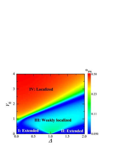
Figure 1: (color online). Ground-state phase diagram of a moving impurity in a quasi-disordered Fermi system, as functions of a $p$-wave pairing parameter $\Delta$ and a disorder strength $V_{0}$, both of which are measured in units of the hopping amplitude $t$. The color in the logarithmic scale represents the value of the inverse participation ratio $\alpha_{\texttt{IPR}}$ of the impurity wave function, from which one may identify two extended phases (I and II) and two localized phases (III and IV). Here, we set the length of the system $L=21$ and the offset phase of the disorder potential $\theta=\pi/(2L)$. The interaction strengths between impurity and fermions are $U_{1}=U_{2}=2t$.

The purpose of this work is two-fold. First, we aim to determine the ground-state phase diagram of the generalized AAH model by introducing a mobile impurity that creates the so-called quasiparticle “polaron” as a probe FChevy2010 ; PMassignan2014 . In condensed matter community, a quenched static impurity has been widely applied as an important local probe that characterizes the underlying nature of the hosting quantum many-body systems AVBalatsky2006 . For example, individual impurity has been experimentally implemented to determine the superconducting pairing symmetry of high-temperature superconductors EWHudson2001 and has been theoretically proposed to probe topological superfluidity HHu2013 . Here, using a mobile impurity (and the corresponding polaron) as a probe is similar to a static one, but is sometimes easier to access experimentally, particularly in the highly controllable cold-atom experiments FChevy2010 ; PMassignan2014 , where polaron, either Fermi polaron or Bose polaron, can be easily created, controlled and detected. As a concrete example, we consider a single mobile impurity immersed in a Fermi “sea” of two-component fermionic atoms with p-wave pairing as described by the generalized non-abelian AAH model XCai2013 ; JWang2016 . In addition, there is a tunable contact interaction between impurity and fermionic atoms. We anticipate that the quasiparticle properties of the resulting polaron should strongly depend on the underlying phases of the non-abelian AAH model. Therefore, by measuring these quasiparticle properties (such as the polaron energy and residue) via radio-frequency spectroscopy, we can map out the ground-state phase diagram of the non-abelian AAH model at zero temperature. Second, we wish to understand how the MBL transition is affected by the $p$-wave superfluidity in the non-abelian AAH model. At infinite temperature, a polaron presents one of the simplest many-body localization system HHu2016 . The polaron may become localized with a strong enough interaction between impurity and fermionic atoms, the phase transition thus provides important information of the interplay between the topological superfluidity and localization.

Our main results on the ground polaron state are briefly summarized in Fig. 1. We can distinguish four different phases by the IPR of the polaron ground state. In phases I and II, the background AAH system is extended and the polaron IPR depends on the size of the system $L$ and behaves like $1/L$. The IPR thus decreases to zero when the system size is large enough. In phase IV, the system becomes localized and the polaron IPR remains to be a finite value that is independent of the system size. Interestingly, in phase III, the polaron IPR exhibits a suppression with respect to the system size $L$, but eventually approaches a finite but small value in the thermodynamic limit $L\rightarrow\infty$. We name it as a weakly-localized phase and interpret it as a direct reflection of the critical phase of the background AAH system. As a result, the large critical area in the non-abelian AAH model due to the $p$-wave superfluidity may be easily identified through the measurement of the IPR of the polaron.

At infinite temperature, on the other hand, the MBL transition is also significantly affected by the existence of $p$-wave pairing. We find that the introduction of a $p$-wave superfluidity usually delocalizes the MBL state and makes the system easier to thermalize, i.e., the critical disorder strength for the MBL transition increases rapidly with increasing $p$-wave pairing (not shown in Fig. 1).

The remainder of this paper is organized as follows: In Sec. II, we outline the model. In Sec. III, we describe the details of a variational approach to solve the single polaron problem, which was developed by Chevy a decade ago. We also describe our diagnostics for determining the localization of the ground polaron state and the many-body localization at infinite temperature. In Sec. IV and Sec. V, we discuss the numerical results of the polaron ground state and many-body localization, respectively. Finally, we conclude in Sec. VI.

II The model

Our system consists a mobile impurity immersed in a sea of noninteracting two-component fermionic atoms loaded into a 1D non-abelian quasi-disordered lattice. The system can be described by the model Hamiltonian,

$$\mathcal{H}=\mathcal{H}_{0}+\mathcal{H}_{1},$$ (1)

where

$$\mathcal{H}_{0}=\sum_{n=1}^{L}\left[\left(\mathbf{c}_{n+1}^{\dagger}\hat{T}_{1}\mathbf{c}_{n}+\textrm{H.c.}\right)+V_{n}\mathbf{c}_{n}^{\dagger}\hat{T}_{2}\mathbf{c}_{n}\right]$$ (2)

is the simplest non-Abelian AAH model JWang2016 with a two-component annihilation field operator $\mathbf{c}_{n}\equiv(c_{n,\uparrow},c_{n,\downarrow})$ and SU($N=2$) hopping matrices

$$\hat{T}_{1}=t\sigma_{z}-\text{$i$$\Delta\sigma$}_{y}$$ (3)

and

$$\hat{T}_{2}=t\sigma_{z}.$$ (4)

Here $\sigma_{z}$ and $\sigma_{y}$ are the usual 2 by 2 Pauli matrices, and $t$ is the hopping amplitude between the nearest-neighboring lattice sites and is set as the unit of energy (i.e., $t=1$). The quasi-disorder lattice is characterized by

$$V_{n}=2V_{0}\cos\left(2\pi n\beta+\theta\right),$$ (5)

where $V_{0}\geq 0$ is the amplitude of the quasi-disorder, $\beta$ is an irrational number that determines the quasi-periodicity, and $\theta$ is an offset phase. If $\Delta=0$, this model $\mathcal{H}_{0}$ reduces to two identical copies of the well-known AAH Hamiltonian (i.e., one copy for each component). In the case that $\Delta>0$, $\mathcal{H}_{0}$ is invariant under the particle-hole transformation, i.e., $c_{n,\uparrow}\leftrightarrow c_{n,\downarrow}^{\dagger}$. The two spin components of the system can then be viewed as the particle and hole components of a spinless $p$-wave superfluid and the parameter $\Delta$ can be conveniently regarded as the $p$-wave pairing JWang2016 . Therefore, we term the model $\mathcal{H}_{0}$ as the generalized AAH model with $p$-wave superfluity. There are four phases in the model $\mathcal{H}_{0}$ separated by three critical lines ($V_{0}=t+\Delta$ or $V_{0}=\left|t-\Delta\right|$) (see Fig. 1 in Ref. JWang2016 for details). For strong quasi-disorder strength $V_{0}>t+\Delta$, all the states of the system are localized and the system is topologically trivial XCai2013 . For small quasi-disorder strength $V_{0}<\left|t-\Delta\right|$, all the states are extended and the system is topologically non-trivial. At last, for a moderate quasi-disorder strength $\left|t-\Delta\right|<V_{0}<t+\Delta$, the three separation lines enclose a large critical area, in which all the states of the system are multifractal.

In Eq. (1), $\mathcal{H}_{1}$ describes the motion of the impurity and its interactions with fermionic atoms in the lattice,

$$\mathcal{H}_{1} = \sum_{n=1}^{L}\left[U_{1}c_{n,\uparrow}^{\dagger}c_{n,\uparrow}d_{n}^{\dagger}d_{n}+U_{2}c_{n,\downarrow}^{\dagger}c_{n,\downarrow}d_{n}^{\dagger}d_{n}\right]$$ (6)

$$+t_{d}\left(d_{n+1}^{\dagger}d_{n}+d_{n}^{\dagger}d_{n+1}\right).$$

Here, $d_{n}$ is the the annihilation field operator for impurity and $U_{1(2)}$ represents the interactions between impurity and atoms with spin up (down). In this work, we mainly focus on the case that the interactions are repulsive ($U_{1,2}>0$) and equal ($U_{1}=U_{2}$). We assume that the impurity is not affected by the quasi-periodic potential and can move freely through the lattice with a hopping amplitude $t_{d}=t$.

Following the typical choice in the literature, for the quasi-disorder potential, we use an irrational number $\beta=(\sqrt{5}-1)/2$, which is the inverse of the golden mean. It can be gradually approached by using the series of Fibonacci numbers $F_{l}$:

$$\beta=\lim_{l\rightarrow\infty}\frac{F_{l-1}}{F_{l}},$$ (7)

where $F_{l}$ is recursively defined by the relation $F_{l+1}=F_{l}+F_{l-1}$, starting from $F_{0}=F_{1}=1$. Thus, in numerical calculations we take the rational approximation: $\beta\simeq\beta_{l}=F_{l-1}/F_{l}$. To minimize the possible effect of the boundary, we take the periodic boundary condition (i.e., $c_{n+L,\sigma}=c_{n,\sigma}$ and $d_{n+L}=d_{n}$) and assume that the length of the system $L$ is periodic with a period $F_{l}$.

III Chevy’s variational approach

Inspired by the great success of Chevy ansatz in solving the polaron problems PMassignan2014 ; FChevy2006 , in this section we diagonalize the impurity Hamiltonian Eq. (1) by using the same variational ansatz in real space bases, within the one particle-hole approximation.

III.1 Chevy ansatz with one particle-hole excitation

For the non-Abelian AAH model $\mathcal{H}_{0}$ with a two-component field operator, expanding the wave-function in real space bases in the form JWang2016 ,

$$|\psi\rangle=\sum_{n=1}^{L}\left[u_{n}c_{n,\uparrow}+v_{n}c_{n,\downarrow}\right]|0\rangle,$$ (8)

we can diagonalize the model Hamiltonian $\mathcal{H}_{0}$ in Eq. (2) to obtain all the eigenvalues $E_{\eta}$ and the corresponding eigenvectors JWang2016

$$\psi_{\eta}=\left[u_{1,\eta},v_{1,\eta},\text{...},u_{\text{$n$,$\eta$}},v_{\text{$n$,$\eta$}},\text{...},u_{\text{$L$,$\eta$}},v_{\text{$L$,$\eta$}}\right]^{T},$$ (9)

where $n$ is the number of the lattice site, and $\eta=1,2,\text{...},2L$ is the index of the $\eta$-th single-particle state of atoms, and $u_{n,\eta}$ and $v_{n,\eta}$ are the corresponding $\eta$-th wavefunction at the $n$-th site. By denoting $c_{\eta}$ as the annihilation field operator in the $\eta$-th eigenstate, we then have

$$\left\{\begin{array}[]{c}c_{n,\uparrow}=\sum_{\eta=1}^{2L}u_{n,\eta}c_{\eta}\\[5.0pt] c_{n,\downarrow}=\sum_{\eta=1}^{2L}v_{n,\eta}c_{\eta}\end{array}\right..$$ (10)

Therefore, the local density of spin-up and -down atoms at the $n$-th site is,

$$\left\{\begin{array}[]{c}c_{n,\uparrow}^{\dagger}c_{n,\uparrow}=\sum_{\text{$\eta_{1}$$\eta_{2}$}}u_{n,\text{$\eta_{1}$}}^{*}u_{n,\text{$\eta_{2}$}}c_{\eta_{1}}^{\dagger}c_{\eta_{2}}\\[5.0pt] c_{n,\downarrow}^{\dagger}c_{n,\downarrow}=\sum_{\text{$\eta_{1}$$\eta_{2}$}}v_{n,\text{$\eta_{1}$}}^{*}v_{n,\text{$\eta_{2}$}}c_{\eta_{1}}^{\dagger}c_{\eta_{2}}\end{array}\right..$$ (11)

Throughout this work, we consider a Fermi sea of fermionic atoms that are occupied up to the chemical potential $\mu\simeq 0$:

$$|\text{FS}\rangle=\prod_{E_{\eta}<0}c_{\eta}^{\dagger}|0\rangle,$$ (12)

which corresponds to the case of the half-filling of fermionic atoms in the lattice, i.e.,

$$\left\langle c_{n,\uparrow}^{\dagger}c_{n,\uparrow}+c_{n,\downarrow}^{\dagger}c_{n,\downarrow}\right\rangle\simeq 1.$$ (13)

Here, the level index $\eta$ of the single-particle states runs from $1$ (i.e., the ground state) to $L-1$ (i.e., $E_{\eta=L-1}<0$ but $E_{\eta=L}>0$), and, finally, to $2L$ (i.e., the highest energy state). Thus, we obtain the energy of fermionic atoms at zero temperature,

$$E_{\text{FS}}\equiv\sum_{E_{\eta}<0}E_{\eta}.$$ (14)

Following Chevy’s variational approach, we take into account only single particle-hole pair excitation. A mobile impurity may then be described by the following approximate many-body wave function in real space:

$$|\mathcal{P}\rangle=\sum_{n}z_{n}d_{n}^{\dagger}|\text{FS}\rangle+\!\!\!\sum_{\mbox{\tiny$\begin{array}[]{c}n,E_{\text{$\eta_{p}$}}>0\\ E_{\text{$\eta_{h}$}}<0\end{array}$}}\!\!\!\!\alpha_{n}(\text{$\eta_{h}$},\text{$\eta_{p}$})d_{n}^{\dagger}c_{\text{$\eta_{p}$}}^{\dagger}c_{\text{$\eta_{h}$}}|\text{FS}\rangle,$$ (15)

where $z_{n}$ gives the residue of the impurity at each lattice site $n$. The second term with amplitude $\alpha_{n}(\eta_{h},\eta_{p})$ describes the single particle-hole excitation. We note that, the site index $n$ takes $L$ values, the level index $\eta_{h}$ (for hole excitations) runs from $1$ to $L-1$, and $\eta_{p}$ (for particle excitations) takes $L+1$ values. Therefore, the dimension of the whole Hilbert space of Chevy’s ansatz that we will deal with is

$$D=L[1+(L-1)(L+1)]=L^{3}.$$ (16)

Thus, in our calculations, the length of the lattice and the dimension of the Hilbert space are respectively, $L=F_{l=7}=21$ and $D_{l=7}=9,261$, $L=F_{l=8}=34$ and $D_{l=8}=39,304$, $L=F_{l=9}=55$ and $D_{l=9}=166,375$, and $L=F_{l=10}=89$ and $D_{l=10}=2,985,984$.

We also note that, Chevy’s variational ansatz provides an excellent description for both low-lying impurity states (i.e., attractive polarons in the context of a mobile impurity in cold-atoms PMassignan2014 ) and high-lying impurity states (i.e., repulsive polarons).

III.2 Numerical solutions of Chevy’s ansatz

The real space bases of Chevy’s ansatz within the one particle-hole pair approximation is given by, $|i\rangle=d_{n}^{\dagger}|\text{FS}\rangle$ or $|i\rangle=d_{n}^{\dagger}c_{\eta_{p}}^{\dagger}c_{\eta_{h}}|\text{FS}\rangle$, where the index $i$ runs from $1$ to $D$. Although the dimension of the corresponding Hilbert space is still quite large (i.e., $D\sim 10^{4}-10^{6}$), most of the matrix elements of the interaction Hamiltonian $\mathcal{H}_{1}$ are zero. Therefore, the total Hamiltonian $\mathcal{H}=\mathcal{H}_{0}+\mathcal{H}_{1}$ can cast into a sparse matrix that can be easily diagonalized by standard exact diagonalization techniques HHu2016 . To be specific, we have three kinds of matrix elements $\mathcal{H}_{ij}$ :

$$\langle\text{FS}|d_{n}\mathcal{H}d_{n^{\prime}}^{\dagger}|\text{FS}\rangle=\delta_{nn^{\prime}}E_{\text{FS}}+U_{1}\delta_{nn^{\prime}}\sum_{E_{\eta}<0}\left|u_{n,\eta}\right|{}^{2}+U_{2}\delta_{nn^{\prime}}\sum_{E_{\eta}<0}\left|v_{n,\eta}\right|{}^{2}+t_{d}\delta_{n\pm 1,n^{\prime}},$$ (17)

$$\langle\text{FS}|d_{n}\mathcal{H}d_{n^{\prime}}^{\dagger}c_{\eta_{p}^{\prime}}^{\dagger}c_{\eta_{h}^{\prime}}|\text{FS}\rangle=U_{1}\delta_{nn^{\prime}}u_{n,\eta_{p}^{\prime}}u_{n,\eta_{h}^{\prime}}^{*}+U_{2}\delta_{nn^{\prime}}v_{n,\eta_{p}^{\prime}}v_{n,\eta_{h}^{\prime}}^{*},$$ (18)

and

$$\langle\text{FS}|c_{\eta_{h}}^{\dagger}c_{\eta_{p}}d_{n}\mathcal{H}d_{n^{\prime}}^{\dagger}c_{\eta_{p}^{\prime}}^{\dagger}c_{\eta_{h}^{\prime}}|\text{FS}\rangle = \left[\delta_{nn^{\prime}}\left(E_{\text{FS}}+E_{\eta_{p}}-E_{\eta_{h}}\right)+t_{d}\delta_{n\pm 1,n^{\prime}}\right]\delta_{\eta_{p}\eta_{p}^{\prime}}\delta_{\eta_{h}\eta_{h}^{\prime}}$$ (19)

$$+U_{1}\delta_{nn^{\prime}}\left[\delta_{\eta_{p}\eta_{p}^{\prime}}\delta_{\eta_{h}\eta_{h}^{\prime}}\sum_{E_{\eta}<0}\left|u_{n,\eta}\right|{}^{2}+\delta_{\eta_{h}\eta_{h}^{\prime}}u_{n,\eta_{p}}^{*}u_{n,\eta_{p}^{\prime}}-\delta_{\eta_{p}\eta_{p}^{\prime}}u_{n,\eta_{h}^{\prime}}^{*}u_{n,\eta_{h}}\right]$$

$$+U_{2}\delta_{nn^{\prime}}\left[\delta_{\eta_{p}\eta_{p}^{\prime}}\delta_{\eta_{h}\eta_{h}^{\prime}}\sum_{E_{\eta}<0}\left|v_{n,\eta}\right|{}^{2}+\delta_{\eta_{h}\eta_{h}^{\prime}}v_{n,\eta_{p}}^{*}v_{n,\eta_{p}^{\prime}}-\delta_{\eta_{p}\eta_{p}^{\prime}}v_{n,\eta_{h}^{\prime}}^{*}v_{n,\eta_{h}}\right].$$

By using the exact diagonalization technique for a sparse matrix, we can find the ground polaron state on for the lattice size $L$ up to 89 (the corresponding dimension of the Hilbert space is up to several millions) GreenII . However, many disorder realizations are need to address the many-body localization for the excited polaron states in the middle of the many-body spectrum. For convenience, we have used the exact diagonalization routine for a dense matrix and restrict our calculations to $L=13$ (for which the dimension of the corresponding Hilbert space is $D_{l=6}=2,197$).

III.3 Quasi-particle properties of the polaron state

To characterize the quasi-properties of the polaron state, we define a normalized wave function as:

$$\Psi_{n}=\frac{z_{n}}{\sqrt{\mathcal{Z}}},$$ (20)

where $\mathcal{Z}=\sum_{n}z_{n}^{2}$ is the total residue of the polaron state. Moreover, a useful quantity in characterizing the localization properties of the ground polaron state is the inverse participation ratio (IPR). It is given by

$$\alpha_{\textrm{IPR}}=\sum_{n=1}^{L}|\Psi_{n}|^{4},$$ (21)

which measures the inverse of the number of lattice sites being occupied by the moving impurity. In the presence of disorder, for a spatially extended polaron state, it is well known $\alpha_{\textrm{IPR}}\thicksim 1/L$, while for a localized state, $\alpha_{\textrm{IPR}}$ tends to a finite value at the order of $\mathcal{O}(1)$. The $\alpha_{\textrm{IPR}}$ may also have other size dependence that is different from $1/L$ or $\mathcal{O}(1)$, for possible critical states. By tuning the disorder disorder strength, we anticipate a sharp change in $\alpha_{\textrm{IPR}}$, when the system transits from one phase to another. Hence, $\alpha_{\textrm{IPR}}$ can be used to determine the phase boundaries separating the extended, critical, and localized phases.

III.4 The MBL indicator

On the other hand, to investigate the localization properties of high-lying excited polaron states at infinite temperature or MBL, we adopt a common quantum chaos indicator, the average ratio between the smallest and the largest adjacent energy gaps,

$$r_{n}=\frac{\min\left\{\delta_{n}^{E},\delta_{n-1}^{E}\right\}}{\max\left\{\delta_{n}^{E},\delta_{n-1}^{E}\right\}},$$ (22)

where $\delta_{n}^{E}=E_{n}-E_{n-1}$, and $E_{n}$ is the ordered list of many-body energy levels VOganesyan2007 . In the thermalized extended phase, the statistics of the level spacing exhibits a Wigner-Dyson distribution and the average ratio is $r^{\textrm{WD}}\simeq 0.536$, while in the MBL phase, the statistics of the level spacing exhibits a Poisson distribution and the average ratio is $r^{\textrm{P}}=2\ln 2-1\simeq 0.386$ VOganesyan2007 .

IV Phase transitions of the ground polaron state

In this section, we discuss the quasi-particle properties of the moving impurity in its ground state, through the analyses of the wave-function, inverse participation ratio, energy and residue, as functions of the disorder strength $V_{0}$, pairing parameter $\Delta$, and atom-impurity interactions $U_{1}$ and $U_{2}$. This leads to our main result of the ground-state phase diagram as shown in Fig. 1.

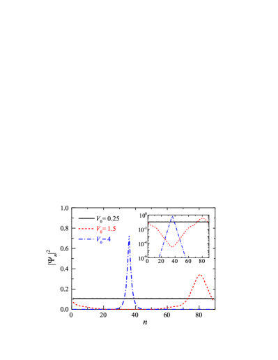
Figure 2: (color online). The amplitude of the wave function of the ground polaron state, at three different disorder strengths as indicated. The inset shows the amplitude in logarithmic scale. Here, we set the length of the system $L=89$ and the offset phase $\theta=\pi/(2L)$. The $p$-wave pairing parameter is $\Delta=2t$ and the interaction strengths between impurity and fermions are $U_{1}=U_{2}=2t$.

IV.1 The wave function and inverse participation ratio

Figure 2 reports typical wave-functions of the ground polaron state in the three different phases for the system length $L=89$, as we observe with increasing disorder strengths at a nonzero $p$-wave pairing parameter $\Delta=2t$ and at the atom-impurity interaction strengths $U_{1}=U_{2}=2t$. At small disorder ($V_{0}=0.25t$, black solid line), the normalized occupation amplitude of the polaron is nearly a constant at each site, suggesting that the polaron state is extended. At a larger disorder strength ($V_{0}=1.5t$, red dashed line), however, this uniform distribution changes into a broad peak located near the site $n=80$. Although the occupation amplitude away from the peak is tiny, it is not exponentially small, as can be seen from the inset of Fig. 2. It thus seems reasonable to treat such a state as a weakly-localized state. At an even larger disorder strength ($V_{0}=4t$, blue dot-dashed line), the peak position moves to the site $n\sim 37$ and the width of the peak becomes much narrower. In addition, away from the peak the occupation amplitude of the polaron decays exponentially (see the blue dot-dashed line in the inset), indicating the appearance of a fully or strongly localized state.

We remark here that the value of the peak position is of little importance. In our calculations, a periodic boundary condition is always assumed and the position of the peak, if exists, is determined by the offset phase $\theta$, which sets a preferable potential minimum. Therefore, one can shift the peak position by simply taking a different offset phase. We also emphasize that the observed localization of the occupation amplitude of the polaron is induced by interactions between impurity and fermionic atoms, as the impurity itself does not experience the quasi-random disorder potential.

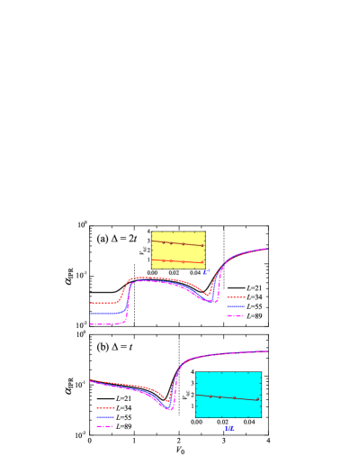
Figure 3: (color online). The inverse participation ratio $\alpha_{\textrm{IPR}}$ as a function of the quasidisorder strength $V_{0}$ at two $p$-wave pairing parameters: $\Delta=2t$ (a) and $\Delta=t$ (b). The different lines correspond to the different sizes of the system, as indicated. As $V_{0}$ increases, one may identify transitions at some critical disorder strengths. The two insets reports the length dependence of the critical strength $V_{0,C}$ and the dashed lines indicate $V_{0,C}$ in the thermodynamic limit $L\rightarrow\infty$. In all the cases, $U_{1}=U_{2}=2t$ and $\theta=\pi/(2L)$.

It is thus clear that with increasing disorder strength, there are transitions between phases with different localization properties. As the localization properties of a single-particle state can be conveniently represented by an inverse participation ratio $\alpha_{\textrm{IPR}}$, in Fig. 3(a) we report $\alpha_{\textrm{IPR}}$ as a function of the disorder strength at $\Delta=2t$. Four different system sizes have been considered, ranging from $L=21$ to $L=89$. It can be seen that the general behavior of the inverse participation ratio is rather independent on the system size $L$: $\alpha_{\textrm{IPR}}$ is initially a constant with increasing disorder strength; At a threshold, it then jumps suddenly; As the disorder strength increases further, $\alpha_{\textrm{IPR}}$ decreases gradually and exhibits a local minimum before finally rises and saturates towards a length-independent value. This general behavior is consistent with the existence of two phase transitions between three typical wave functions shown in Fig. 2.

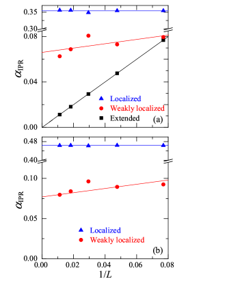
Figure 4: (color online). The length dependence of the inverse participation ratio $\alpha_{\textrm{IPR}}$ in different phases at two $p$-wave pairing parameters: $\Delta=2t$ (a) and $\Delta=t$ (b). The black squares, red circles and blue triangles correspond to the selected cases of extended phase ($V_{0}=0.25t$), weakly localized phase ($V_{0}=1.5t$ in (a) and $V_{0}=t$ in (b)) and strongly localized phase ($V_{0}=4t$ in both (a) and (b)), respectively. For other parameters, we take $U_{1}=U_{2}=2t$ and $\theta=\pi/(2L)$.

For a given $L$, intuitively we may define the inflection point of the jump and the position of the local minimum as the critical disorder strengths for the two transitions. In the inset of Fig. 3(a), we show the critical disorder strengths as a function of the inverse system size $L^{-1}$. In the thermodynamic limit of $L\rightarrow\infty$, the critical disorder strengths approach $V_{0,C}=t$ and $V_{0,C}=3t$, respectively. Interestingly, these two critical disorder strengths are exactly identical to the two thresholds of the background generalized AAH model with $p$-wave superfluidity that separate the extended, critical and localized single-particle states, which are given by $\left|t-\Delta\right|$ and $t+\Delta$ JWang2016 , respectively. By varying the $p$-wave pairing parameter $\Delta$, we have checked that this identicalness actually holds for any values of $\Delta$. In Fig. 3(b), we provide another example at $\Delta=t$. In this case, the first critical disorder strength decreases to $V_{0,C}=\left|t-\Delta\right|=0$ and therefore cannot be identified from the plot.

As a brief conclusion, we find that the moving impurity or polaron in the ground state shares a similar phase diagram as the background fermionic atoms, which has already been illustrated by the figure of $\alpha_{\textrm{IPR}}$ in logarithmic scale for a small system size $L=21$, as shown in Fig. 1. This is a very useful observation, since it is then reasonable to anticipate that the measurements of the polaron quasi-particle properties, such as its energy and residue, could provide a useful probe of the background non-abelian AAH model with $p$-wave superfluidity.

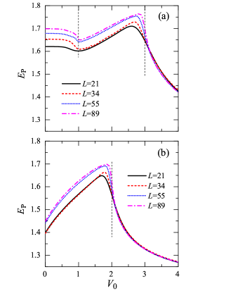
Figure 5: (color online). The polaron energy $E_{P}$ as a function of the quasidisorder strength $V_{0}$ at two $p$-wave pairing parameters: $\Delta=2t$ (a) and $\Delta=t$ (b). The different lines correspond to the different sizes of the system, as indicated. Here, we take $U_{1}=U_{2}=2t$ and $\theta=\pi/(2L)$.

The only difference between the two phase diagrams is that the critical phase in the non-abelian AAH model, enclosed by the curves $\left|t-\Delta\right|$ and $t+\Delta$, has now been replaced by the weakly localized phase of the polaron. This is not surprising, since in some sense the critical phase of fermionic atoms is fragile and may not be mirrored by the polaron. To confirm it, we check the inverse participation ratio $\alpha_{\textrm{IPR}}$ of the three typical wave-functions in the thermodynamic limit $L\rightarrow\infty$. As shown in Fig. 4(a), $\alpha_{\textrm{IPR}}$ of the extended state (black squares) vanishes linearly as a function of $1/L$. On the contrary, $\alpha_{\textrm{IPR}}$ of the localized state (blue triangles) takes a finite value at the order of $\mathcal{O}(1)$ and is essentially unchanged with decreasing $1/L$. The intermediate state (red circles) seems to have much smaller $\alpha_{\textrm{IPR}}$ than the localized state. But, it does not vanish as $L^{-1}\rightarrow 0$, unlike a critical phase. This justifies the use of our terminology of a weakly localized state.

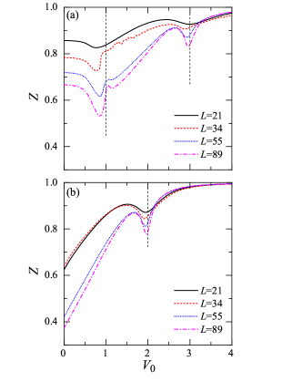
Figure 6: (color online). The polaron residue $\mathcal{Z}$ as a function of the quasidisorder strength $V_{0}$ at two $p$-wave pairing parameters: $\Delta=2t$ (a) and $\Delta=t$ (b). The different lines correspond to the different sizes of the system, as indicated. Here, we take $U_{1}=U_{2}=2t$ and $\theta=\pi/(2L)$.

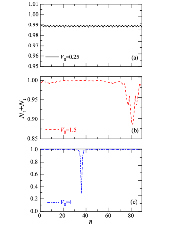
Figure 7: (color online). The occupation number of fermionic atoms at three different disorder strengths: (a) $V_{0}=0.25t$, (b) $V_{0}=1.5t$, and (c) $V_{0}=4t$. Here, we set the length of the system $L=89$ and the offset phase $\theta=\pi/(2L)$. The $p$-wave pairing parameter is $\Delta=2t$ and the interaction strengths between impurity and fermions are $U_{1}=U_{2}=2t$.

IV.2 The polaron energy and residue

Fig. 5 and Fig. 6 present the polaron energy $E_{P}=E-E_{\textrm{FS}}-E_{\textrm{imp}}^{(0)}$ and the polaron residue $\mathcal{Z}$ as a function of the disorder strength at $U_{1}=U_{2}=2t$, respectively. Here, $E$ is the energy of the ground state obtained by exact diagonalization and $E_{\textrm{imp}}^{(0)}=-2t_{d}=-2t$. As anticipated, both energy and residue show non-monotonic dependences on the disorder strength, which are consistent with the existence of some phase transitions. Let us focus on the energy at $\Delta=2t$, as shown in Fig. 5(a). At small disorder, the energy of the polaron slowly decreases with increasing disorder strength. This is because in the extended state, the fermionic atoms and impurity are miscible and are able to optimize their distance to reduce the repulsive interaction energy. At large disorder, the energy again decreases as the disorder strength increases. In this limit, the atoms and impurity are essentially phase separated. This is evident by comparing the blue dot-dashed lines in Fig. 7(c) and in Fig. 2, which show the atomic density distribution and the impurity density distribution, respectively. The phase separation favors a small repulsive interaction energy, which in turns provides a mechanism for the full localization of the polaron. At an intermediate disorder strength (i.e., $t<V_{0}<3t$ in Fig. 5(a)), the system is actually frustrated. The fermionic atoms and impurity try to avoid each other to reduce the interaction energy, but the strength of the disorder is not large enough to create a well-localized polaron state. This leads to a slight oscillation of the atomic density distribution around the impurity, as can be seen from Fig. 7(b). The frustration is responsible for the enhancement of the polaron energy shown in 5(a), as the disorder strength increases.

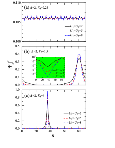
Figure 8: (color online). The amplitude of the wave function of the ground polaron state at three different disorder strengths: (a) $V_{0}=0.25t$, (b) $V_{0}=1.5t$, and (c) $V_{0}=4t$ and at three different interaction strengths as indicated. The inset in (b) shows the amplitude in logarithmic scale. Here, we set the length of the system $L=89$ and the offset phase $\theta=\pi/(2L)$. The $p$-wave pairing parameter is $\Delta=2t$.

IV.3 The dependence on the atom-impurity interaction

We consider so far for the case of fixed atom-impurity interaction strengths $U_{1}=U_{2}=2t$. Nevertheless, the phase diagram of the ground polaron state does not change if we take larger interaction strength. In Fig. 8, we report the three typical wave-functions at different interaction strengths. In the extended phase (a), the wave-function is basically unchanged upon increasing interaction strength. On the other hand, in the weakly localized phase (b) or the localized phase (c), the interaction strength tends to sharpen the localization peak and hence make the state more localized. One may expect that the weakly localized phase turns into a well localized phase at sufficiently large interaction strength. This seems unlikely, however, since the full width at half maximum (FWHM) of the peak of the weakly localized phase does not decrease too much with increasing interaction strength. It remains large at $U_{1}=U_{2}=8t$ (i.e., $\sim 10$ sites), much larger than that of a fully localized phase (i.e., $\sim 2$ sites)

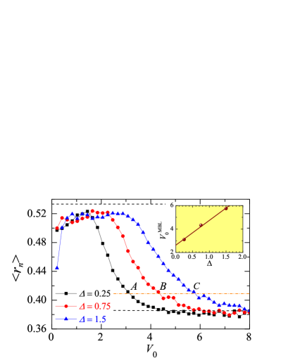
Figure 9: (color online). The averaged ratio of adjacent energy gaps $\langle r_{n}\rangle$ as a function of the disorder strength at different values of the $p$-wave pairing parameter $\Delta$. The average is calculated over the central half of the spectrum, averaging over 100 quasi-random disorder realizations, by randomly generating the phase offset $\theta$. The two dashed lines show the anticipated average ratios for the Wigner-Dyson distribution ($r^{\textrm{WD}}=0.536$) and for the Poisson distribution ($r^{\textrm{P}}=0.386$), respectively. The dot-dashed line indicates a critical averaged ratio $\langle r_{n}\rangle_{\textrm{MBL}}=0.41$, below which all the states of the polaron may become localized, i.e., MBL occurs. The inset shows the critical disorder strength for MBL as a function of the pairing parameter $\Delta$, with a straight line as a guide to the eye. Here, we take $U_{1}=U_{2}=2$ and a small system size $L=13$.

V many-body localization of the excited polaron states

We now turn to consider the localization of the high-energy polaron states or MBL. A convenient way to identify the MBL is to calculate the averaged ratio of adjacent energy levels, which is defined in Eq. (22). In Fig. 9, we report the averaged ratio $\langle r_{n}\rangle$ as a function of the disorder strength for different values of the $p$-wave pairing parameter $\Delta$. Here, we take $U_{1}=U_{2}=2$ and $L=13$. The three different lines correspond to the different values of $\Delta$. The two horizontal dashed lines show the averaged ratio for the Wigner-Dyson distribution ($r^{\textrm{WD}}\simeq 0.536$) and for the Poisson distribution ($r^{\textrm{P}}\simeq 0.386$), respectively. Quite generally, we find that when the disorder is weak, $\langle r_{n}\rangle$ tends to $r^{\textrm{WD}}$, which means the system can be thermalized. In contrast, when the disorder is strong, $\langle r_{n}\rangle$ approaches $r^{\textrm{P}}$, indicating the appearance of MBL.

It is readily seen that the averaged ratio depends sensitively on the pairing parameter. By increasing $\Delta$, the curve is shifted horizontally to the right side of the figure. The system thus seems to become more difficult to be many-body localized as $\Delta$ increases. To have a qualitative characterization, we may estimate the critical disorder strength of MBL, $V_{0}^{\textrm{MBL}}$, by using the criterion,

$$\left\langle r_{n}\right\rangle(V_{0}^{\textrm{MBL}})=0.41.$$ (23)

This naïve estimation is qualitative only and is motivated by the fact that the MBL in the disordered spin-chain VOganesyan2007 ; DJLuitz2015 and Hubbard models RMondaini2015 occurs at a similar averaged ratio $\left\langle r_{n}\right\rangle_{\textrm{MBL}}\sim 0.41$. In the figure, we show this MBL averaged ratio by a dot-dashed line and determine $V_{0}^{\textrm{MBL}}$ at the three pairing parameters from the three cross points, labelled as $A$, $B$ and $C$, respectively. As shown in the inset, roughly speaking, the critical disorder strength for MBL $V_{0}^{\textrm{MBL}}$ depends linearly on the $p$-wave pairing parameter $\Delta$.

VI Conclusions

In summary, we have theoretically investigated the ground-state and excited states properties of a mobile impurity or polaron immersed in a one-dimensional quasiperiodic Fermi system with topological $p$-wave superfluidity. On the one hand, for the ground state we find four distinct phases of the polaron: two extend phases, a weakly localized phase and a localized phase (see Fig. 1), according to the inverse participation ratio of the polaron wave-function. This phase diagram of the polaron is a perfect mirror of the phase diagram of the background fermionic atoms, which is described by the non-abelian Aubry-André-Harper model. As a result, experimentally we may probe the phase diagram of the non-abelian AAH model by measuring the quasi-particle properties of the polaron. On the other hand, we have briefly considered the many-body localization of the excited polaron states at infinite temperature. We find that the existence of a $p$-wave pairing parameter helps delocalize MBL and makes the system easier to thermalize.

- (1) P. W. Anderson, Phys. Rev. 109, 1492 (1958).
- (2) R. Dalichaouch, J. P. Armstrong, S. Schultz, P. M. Platzman, and S. L. McCall, Nature (London) 354, 53 (1991).
- (3) A. A. Chabanov, M. Stoytchev, and A. Z. Genack, Nature (London) 404, 850 (2000).
- (4) T. Schwartz, G. Bartal, S. Fishman, and M. Segev, Nature (London) 446, 52 (2007).
- (5) Y. Lahini, A. Avidan, F. Pozzi, M. Sorel, R. Morandotti, D. N. Christodoulides, and Y. Silberberg, Phys. Rev. Lett. 100, 013906 (2008).
- (6) J. Billy, V. Josse, Z. Zuo, A. Bernard, B. Hambrecht, P. Lugan, D. Clement, L. Sanchez-Palencia, P. Bouyer, and A. Aspect, Nature (London) 453, 891 (2008);
- (7) G. Roati, C. D’Errico, L. Fallani, M. Fattori, C. Fort, M. Zaccanti, G. Modugno, M. Modugno, and M. Inguscio, Nature (London) 453, 895 (2008).
- (8) M. Rigol, V. Dunjko, and M. Olshanii, Nature (London) 452, 854 (2008).
- (9) A. Polkovnikov, K. Sengupta, A. Silva, and M. Vengalattore, Rev. Mod. Phys. 83, 863 (2011).
- (10) J. M. Deutsch, Phys. Rev. A 43, 2046 (1991).
- (11) M. Srednicki, Phys. Rev. E 50, 888 (1994).
- (12) R. Nandkishore and D. A. Huse, Annu. Rev. Condens. Matter Phys. 6, 15 (2015).
- (13) E. Altman and R. Vosk, Annu. Rev. Condens. Matter Phys. 6, 383 (2015).
- (14) A. Pal and D. A. Huse, Phys. Rev. B 82, 174411 (2010).
- (15) J. H. Bardarson, F. Pollmann, and J. E. Moore, Phys. Rev. Lett. 109, 017202 (2012).
- (16) R. Vosk and E. Altman, Phys. Rev. Lett. 110, 067204 (2013).
- (17) M. Serbyn, Z. Papic, and D. A. Abanin, Phys. Rev. Lett. 110, 260601 (2013).
- (18) F. Andraschko, T. Enss, and J. Sirker, Phys. Rev. Lett. 113, 217201 (2014).
- (19) M. Schreiber, S. S. Hodgman, P. Bordia, H. P. Lüschen, M. H. Fischer, R. Vosk, E. Altman, U. Schneider, and I. Bloch, Science 349, 842 (2015).
- (20) P. G. Harper, Proc. Phys. Soc. London, Sect. A 68, 874 (1955).
- (21) S. Aubry and G. André, Ann. Israel Phys. Soc. 3, 133 (1980).
- (22) S. Iyer, V. Oganesyan, G. Refael, and D. A. Huse, Phys. Rev. B 87, 134202 (2013).
- (23) S. Ostlund, R. Pandit, D. Rand, H. J. Schellnhuber, and E. D. Siggia, Phys. Rev. Lett. 50, 1873 (1983).
- (24) M. Kohmoto, Phys. Rev. Lett. 51, 1198 (1983).
- (25) D. J. Thouless, Phys. Rev. B 28, 4272 (1983).
- (26) J. H. Han, D. J. Thouless, H. Hiramoto, and M. Kohmoto, Phys. Rev. B 50, 11365 (1994).
- (27) I. Chang, K. Ikezawa, and M. Kohmoto, Phys. Rev. B 55, 12971 (1997).
- (28) Y. Takada, K. Ino, and M. Yamanaka, Phys. Rev. E 70, 066203 (2004).
- (29) F. Liu, S. Ghosh, and Y. D. Chong, Phys. Rev. B 91, 014108 (2015).
- (30) L.-J. Lang, X. Cai, and S. Chen, Phys. Rev. Lett. 108, 220401 (2012).
- (31) Y. E. Kraus and O. Zilberberg, Phys. Rev. Lett. 109, 116404 (2012).
- (32) S.-L. Zhu, Z.-D.Wang, Y.-H. Chan, and L.-M. Duan, Phys. Rev. Lett. 110, 075303 (2013).
- (33) W. DeGottardi, D. Sen, and S. Vishveshwara, Phys. Rev. Lett. 110, 146404 (2013).
- (34) X. Cai, L.-J. Lang, S. Chen, and Y. Wang, Phys. Rev. Lett. 110, 176403 (2013).
- (35) F. Grusdt, M. Honing, and M. Fleischhauer, Phys. Rev. Lett. 110, 260405 (2013).
- (36) I. I. Satija and G. G. Naumis, Phys. Rev. B 88, 054204 (2013).
- (37) R. Barnett, Phys. Rev. A 88, 063631 (2013).
- (38) X. Deng and L. Santos, Phys. Rev. A 89, 033632 (2014).
- (39) J. Wang, X.-J. Liu, G. Xianlong, and H. Hu, Phys. Rev. B 93, 104504 (2016).
- (40) Q.-B. Zeng, S. Chen, and R. Lü, Phys. Rev. A 95, 062118 (2017).
- (41) F. Chevy and C. Mora, Rep. Prog. Phys. 73, 112401 (2010).
- (42) P. Massignan, M. Zaccanti, and G. M. Bruun, Rep. Prog. Phys. 77, 034401 (2014).
- (43) A. V. Balatsky, I. Vekhter, and J.-X. Zhu, Rev. Mod. Phys. 78, 373 (2006).
- (44) E. W. Hudson, K. M. Lang, V. Madhavan, S. H. Pan, H. Eisaki, S. Uchida, and J. C. Davis, Nature (London) 411, 920 (2001).
- (45) H. Hu, L. Jiang, H. Pu, Y. Chen, and X.-J. Liu, Phys. Rev. Lett. 110, 020401 (2013).
- (46) H. Hu, A. B. Wang, S. Yi, and X.-J. Liu, Phys. Rev. A 93, 053601 (2016).
- (47) F. Chevy, Phys. Rev. A 74, 063628 (2006).
- (48) For more details on Swinburne supercomputer Green II resource, we refer to the homepage, http://supercomputing.swin.edu.au/.
- (49) V. Oganesyan and D. A. Huse, Phys. Rev. B 75, 155111 (2007).
- (50) D. J. Luitz, N. Laflorencie, and F. Alet, Phys. Rev. B 91, 081103(R) (2015).
- (51) R. Mondaini and M. Rigol, Phys. Rev. A 92, 041601(R) (2015).