Strong entanglement of spins inside a quantum domain wall

Abstract

Magnetic domain walls (DWs) are widely regarded as classical objects in physics community, even though the concepts of electron spins and spin-spin exchange interaction are quantum mechanical in nature. One intriguing question is whether DWs can survive at the quantum level and acquire the quantum properties such as entanglement. Here we show that spins within a DW are highly entangled in their quantum description. The total magnetization of a magnetic DW is nonzero, which is a manifestation of the global entanglement of the collective spin state. These results significantly deepen our understanding of magnetic DWs and enable the application of DWs in quantum information science. The essential physics can be generalized to skyrmions so that they can also play a role in quantum information processing.

Entanglement is a measure of quantum correlations between two or among more than two quantum particles. It is a natural resource for quantum computing and quantum information processing. Finding/generating, extracting and utilizing this resourse is an important task in quantum information scienceNielsen . Entangling tens particles have been realized experimentally Neeley2010 ; DiCarlo2010 ; Barends2014 ; Bernien2017 ; Zhang2017 ; Song2017 . Remarkably, in superconducting circuits and trapped ions, it is now possible to control and to tune the coupling strength between two spins from ferromagnetic to antiferromagnetic interactions. These developments open intriguing possibilities for studying the quantum properties of magnetic structures, such as DWs Hubert ; Yuan2015 ; Yuan2016nonlocal , vortices Shinjo2001 ; Wachowiak2002 ; Choe2004 ; Yuan2015guide and even skyrmions Bogdanov2001 ; Rosler2006 ; Muhlbauer2009 ; Yu2010 ; yuan2016 with a finite number of controllable spins. To initiate this interdisciplinary field, it is essential to connect magnetic structures with the measurable quantities of quantum information, such as purity of spins and global entanglement of the system yuan2017bec .

Here we study a quantum magnetic wire with two magnetic domains and a DW in between. We show that all spins in the DW are highly entangled. The net magnetization of DWs does not depend on the nanowire length and it can be well characterized by the global entanglement of the system. In addition, we find that global entanglement of the system is a natural indictor of the phase transition between quantum DWs and domains.

Results

Model of quantum domain walls. Let us consider the transverse Ising model of $N$ spin-1/2 particles on a one dimensional (1D) lattice, subject to boundary fields $h$, the Hamiltonian reads

$$\mathcal{H}=J\sum_{\langle ij\rangle}\sigma_{i}^{z}\cdot\sigma_{j}^{z}-g\sum_{i=1}^{N}\sigma_{i}^{x}-h(\sigma_{1}^{z}+\sigma_{N}^{z}),$$ (1)

where $\sigma_{i}^{x},\sigma_{i}^{z}$ are the Pauli matrices on the $i$-th site, $J$ is the exchange coupling and $g$ is the anisotropy energy. Here $\langle ij\rangle$ denotes nearest neighbor spins. The ground-state energy $E_{0}$ and the corresponding ground state $|0\rangle$ is calculated using the standard Lancoz algorithm Lanczos1950 ; Dagotto1994 (See Methods for details), which is double checked by the exact diagonization of the Hamiltonian $\mathcal{H}$ for $N\leq 8$.

In the following, we shall focus on the antiferromagnetic (AFM) coupling ($J>0$) for an illustration and discussion of our results. The conclusions drawn below can be generalized to the ferromagnetic coupling as well. In an AFM domain, the quantum version of the magnetization order $m_{i}^{z}$ and Néel order $n_{i}^{z}$ Yuan2017direction is given by the following expectation values:

$$m_{i}^{z}=\frac{1}{2}\langle 0|\sigma_{i}^{z}+\sigma_{i+1}^{z}|0\rangle,n_{i}^{z}=\frac{1}{2}\langle 0|\sigma_{i}^{z}-\sigma_{i+1}^{z}|0\rangle,$$ (2)

where $i=1,3,5,...N-1$. Without ambiguity, the number of spins is assumed even and $J=1.0$ if it is not stated otherwise.

Domain wall properties. Let us first look at the numerical results, in the regime with weak anisotropy $g\ll J$. Figure 1a shows the spatial variation of $m_{i}^{z}$ and $n_{i}^{z}$ for $N=12$ (triangles), 16 (circles), 20 (squares), respectively. These profiles are similar to those of classical AFM DWs. (1) The Néel order $n_{z}$ has a typical classical DW profile whose value varies from 1 on the left hand side (LHS) of the chain to $-1$ on the right hand side (RHS). (2) The magnetization order $m_{z}$ is zero in the two domains and reaches its maximum at the DW center. As the system becomes larger, the magnetic moments near the center become smaller, but, by summing all the magnetic moments in the DW, the net magnetization is $m_{t}^{z}=1/2$, independent of the system size ($N$) as shown in the inset of Fig. 1a.

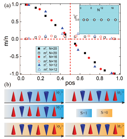
Figure 1: Scheme of quantum domain walls. (a) Spatial variation of $m^{z}$ (open symbols) and $n^{z}$ (filled symbols) for a spin chain with $N=12$ (triangles), 16 (circles), 20 (squares), respectively. The top-right inset shows the net magnetization as a function of $N$. $\mathrm{pos}=i/N$ is the scaled position of the $i-$th site, $g=0.2.$ (b) Scheme of the five degenerated low energy excitation states for $N=6$. The blue (orange) background represents the net magnetization of the corresponding state to be $S=1$ ($S=0$).

To further prove the result of $m_{t}^{z}=1/2$, we look at the structure of a quantum DWs of $N$ spins. The boundary spins are aligned along the $+z$ direction by the external fields. Given $g\ll J$, the AFM exchange interaction dominates the Hamiltonian (1). Thus, the lowest energy states (i.e. ground-state) are those states with only one pair of neighboring spins left alone (sketched as a pair of parallel spins in Fig. 1b) while rest nearest neighboring spins are anti-parallel with each other forming a zero spin singlet state. For $N=6$, there are five such configurations of same energy as sketched in Fig. 1b. In general, there are $N-1$ such states of energy $-(N-3)J$. These states can be further classified into $|\varphi^{S=1}_{i}\rangle$ for $S=1$ and $|\varphi^{S=0}_{i}\rangle$ for $S=0$, $N/2$ for $S=1$ and the remaining for $S=0$, where $S$ is the net magnetization of the system. The true ground state under the boundary conditions is the linear combination of this states. The corresponding eigenstate of the Hamiltonian (1) is

$$|0_{\mathrm{th}}\rangle=\sum_{i=1}^{N/2}a_{i}|\varphi^{S=1}_{i}\rangle+\sum_{i=1}^{N/2-1}b_{i}|\varphi^{S=0}_{i}\rangle\$$ (3)

where $a_{i}$,$b_{i}$ are the superposition coefficients. By rearranging the basis states such that $S=1$ and $S=0$ states are ordered alternatively, the Hamiltonian (1) can be recasted as a tridiagonal-Toeplitz matrix, where the ground state energy is found to be $E_{0}=-(N-3)J-2g\cos\left(\pi/N\right)$ with the wave function

$$|0_{\mathrm{th}\rangle}=\sqrt{\frac{2}{N}}\left(\sin\frac{\pi}{N},\sin\frac{2\pi}{N},...,\sin\frac{(N-1)\pi}{N}\right),$$ (4)

Note that the anisotropy term $g$ only gives a first-order correction of the ground state energy. As a result, the magnetic moments distribution is given by $m_{i}^{z}=\langle 0_{\mathrm{th}}|\sigma_{i}^{z}+\sigma_{i+1}^{z}|0_{\mathrm{th}}\rangle/2=u_{i}$, where $u_{i}=2/N\sin^{2}i\pi/N$. The net magnetization can be calculated as

$$m^{z}_{t}=\sum_{\mathrm{odd}~{}i}^{N-1}u_{i}=\frac{1}{2},$$ (5)

which does not depend on $N$, in agreement with numerical results. The essential physics is that the ground state is a superposition of total spin $S=1$ and $S=0$ configurations with equal contributions ($\sum u_{2i}=\sum u_{2i+1}=1/2$) so that the average spin number is always 1/2.

In fact, the above result is also true when the Dzyaloshinsiki-Moriya interaction (DMI) Dz1957 ; Moriya1960 $H_{\mathrm{DM}}=-\mathbf{D}\cdot\sum_{\langle ij\rangle}\sigma_{i}\times\sigma_{j}$ is added to Hamiltonian (1), where the ground state of the revised Hamiltonian is still solvable analytically. Specifically, for $\mathbf{D}=D\hat{y}\ (D>0)$, the ground state is given by,

$$|0_{\mathrm{th}}\rangle=\sqrt{\frac{2}{N}}\left(\tau_{1}\sin\frac{\pi}{N},\tau_{2}\sin\frac{2\pi}{N},...,\tau_{N-1}\sin\frac{(N-1)\pi}{N}\right),$$ (6)

where the prefactor $\tau_{i}=1-2\ \mathrm{mod}(\lceil i/2\rceil,2)$, $\lceil x\rceil$ is the ceiling function of $x$. Note that $\tau_{i}^{2}=1$, the magnetization distribution $m_{i}^{z}=2/N\sin^{2}(i\pi/N)$, is not changed by the DMI. However, the chirality of DW does depend on the sign of $D$. For $D>0$, the system always prefers a clockwise Néel wall. However, if $D$ reverses the sign, the ground state becomes counter-clockwise. This is consistent with classical case yuan2017 .

Entanglement. In quantum information science, the purity of the $i$-th spin is defined as $P_{i}=\mathrm{tr}(\rho_{i}^{2})$ where $\rho_{i}$ is the density matrix of the $i$-th spin obtained by tracing all the other spins in the full density matrix $|0\rangle\langle 0|$. It quantifies the distance of a state relative to a pure state; for example, it takes the value 1 for a separable pure state, but 1/2 for a maximally entangled states such as Bell states and Greenberg-Horne-Zelinger state (GHZ) states GHZ2007 .

Figure 2a shows the space distribution of purity as colored rectangles for $N=12$ (top inset), $16$ (middle inset), and $20$ (bottom inset), respectively. Regardless of the system size, the purity takes 1 near the boundary of spin chain and then decreases to form a symmetric dip around the chain center at $i/N=1/2$. The magnetization distribution of DWs takes on a peak centered at the dip position and its space dependence is strongly correlated with the purity. Physically, this correlation originates from the antiferromagnetic nature of nearest neighbour interaction. For the spins near the boundary, their directions are strongly bounded by the fixed orientations of the boundary spins and have a larger probability to be in Néel-state-like configurations. Consequently, the magnetization is close to zero and these spins are not entangled with the others (i.e., close to a pure state). The spins near the center are influenced lightly by the boundary spins and their directions become much more uncertain, hence the purity of these spins become smaller. The purity of spins close 1/2 at the wire center suggests that the spins inside the domain walls are highly entangled.

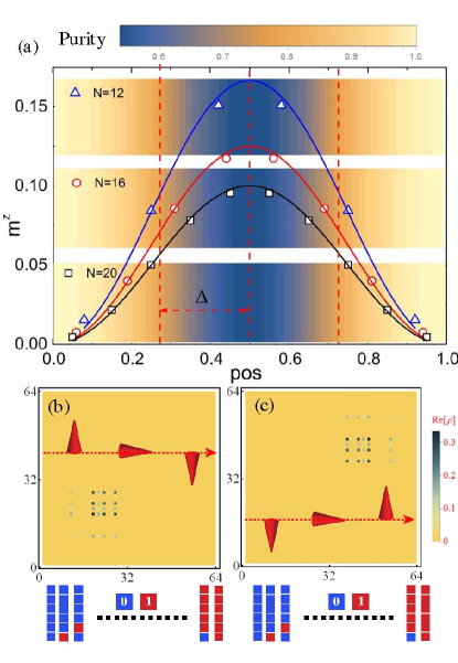
Figure 2: Tomography of quantum domain walls. (a) Distribution of the magnetic moments of DWs for $N=12$ (triangles), $16$ (circles) and $20$ (squares), respectively. The solid lines are the theoretical results given by $m_{i}^{z}=u_{i}$. The colored strips represent the distribution of purity at the corresponding $N$. (b) (c) Density of states tomography for a clockwise/counter-clockwise DW state in a spin chain with $N=6$. The values of vertical/horizontal axis represents the value of the basis vector by treating up spin as bit 0 and down spin as bit 1. The inset sketches the DW profile.

Theoretically, the purity of the $i-$th spin is defined by the reduced density operator of the $i-$th spin obtained by tracing all the spins except the $i-$th spin in density operator $|0_{\mathrm{th}}\rangle\langle 0_{\mathrm{th}}|$ as

$$P_{i}^{\mathrm{th}}=\left(\sum_{k=1}^{i-1}u_{k}\right)^{2}+\left(\sum_{k=i}^{N-1}u_{k}\right)^{2}+2u_{i}u_{i-1},$$ (7)

where $i=1,2,...,N$. The third term $u_{i}u_{i-1}$ is of the order $O(1/N^{2})$, which is much smaller than the first two terms. Considering $\sum u_{i}=1$, $P_{i}$ reaches its minimum value (1/2) at $i=N/2$, i.e. the chain center, where $m_{i}^{z}=u_{i}\propto\sin^{2}(i\pi/N)$ reaches its maximum value.

The correlations of the magnetization distribution and purity distribution can be extended to two dimensions (2D) where rich magnetic structures such as vortices, skyrmions can exist since the physics remain the same. Nevertheless, it is a great challenge to find the ground states in 2D both analytically and numerically. Practically, the correlations also allow us to measure a quantum DW, vortices and even skyrmions by measuring the purity of each spin in a spin chain. The later can be realized by performing state tomography on each system qubit or by a more efficient technique that uses bitwise interactions between the system and identically prepared registers Brennen2003 . A typical tomography of the density of states for a clockwise/counter-clockwise DW is shown in Fig. 2b and 2c. The distinguishable distributions of the density matrix allows us to classify clockwise and counter-clockwise DWs.

Furthermore, the direct sum of magnetization recovers the net magnetization of the spin chain while the proper average of the local purity can give the global entanglement ($E_{g}$) of the spins. The original definition of $E_{g}$ is given by Meyer and Wallach Meyer2002 and then reformulated in terms of the sum of local purity Brennen2003 , i.e.

$$E_{g}\equiv\frac{2}{N}\sum_{i=1}^{N}(1-P_{i}).$$ (8)

Substituting Eq. (7) into this definition, the leading order of global entanglement is reduced to

$$E_{g}=2-\frac{2}{N}\sum_{k=1}^{N}\left[\left(\sum_{i=1}^{k-1}u_{i}\right)^{2}+\left(\sum_{i=k}^{N-1}u_{i}\right)^{2}\right].$$ (9)

The sum increases as $N$ increases and saturates for $N>20$. The limiting value is $E_{g}=2/3-5/2\pi^{2}\approx 0.41$. This indicates that the spins in a DW is still entangled in the macroscopic scale ($N\rightarrow\infty$). This is quite different from a classic DW that has zero entanglement since all its composite spins have definite orientations.

As a comparison, for a quantum domain state without DWs such as the superposition of two degenerated Néel states,

$$|0_{\mathrm{th}}\rangle=\frac{1}{\sqrt{2}}\left(|\uparrow\downarrow\uparrow\downarrow...\uparrow\downarrow\rangle+\right|\downarrow\uparrow\downarrow\uparrow...\downarrow\uparrow\rangle)$$ (10)

The global entanglement is $E_{g}=1$ while its net magnetization is zero. Based on this comparison, it becomes possible to distinguish domain and DW states and the corresponding net magnetization by measuring the global entanglement of the spin system.

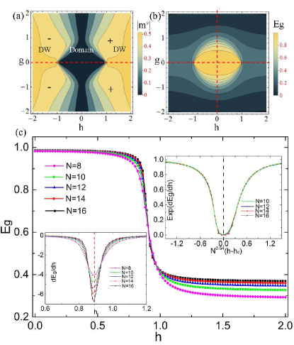
Figure 3: Phase diagram and the characterization of the phase transition using entanglement. (a) The distribution of net magnetization of the spin chain ($|\mathrm{m}^{z}|$) in the $h-g$ phase space. The $\pm$ signs represent clockwise and counter-clockwise DW respectively. $N=12$. (b) Simulated global entanglement ($E_{g}$) distribution in the $h-g$ phase space. (c) Global entanglement ($E_{g}$) as a function of boundary field ($h$). $g=0.2$. Left inset: $dE_{g}/dh$ as a function of external field for $N=8,10,12,14,16$, respectively. Right inset: scaling behavior of the global entanglement around the critical point $h_{c}$.

Phase transition. To know the size of the phase space where the quantum DWs are stable, it is interesting to plot the phase diagram of the spin model. In our numerical simulation, we fix the exchange coupling and adjust the anisotropy $g$ and boundary fields to obtain various ground states in $h-g$ plane as shown in Fig. 3.

Guided by the red line in Fig. 3a, the ground state changes from a single domain state to a quantum DW at the critical field of $h_{c}=J$ for $g=0$. The critical field has a non-trivial dependence on $g$ and $h$. For simplicity, we focus on the regime $g\ll 1$, where the ground state is mainly determined by the competition of exchange interaction and Zeeman interaction. In this regime, the global entanglement ($E_{g}$) shows an abrupt jump from 1.0 to a smaller value as shown in 3b and Fig. 3c with $g=0.2$. This abrupt change is due to the distinguishable quantum properties of the domains and DWs. When $h<h_{c}$, the exchange interaction dominates the Hamiltonian and the ground state is a superposition of two degenerated Néel states Eq. (10) with $E_{g}=1$. The numerical value of $E_{g}$ is a little smaller than the theoretical value 1, as shown in Fig. 3c, due to the influence of the small anisotropy $g$ term, which tendency is to align all the spins to $x$ direction and reduce the entanglement. As the field increases above $h_{c}$, the ground state becomes a DW state with finite entanglement 0.41 as discussed previously.

The global entanglement and its first derivative is continuous with $h$ near the critical field while its second order derivative is discontinuous, as shown in the left inset of Fig. 3c. To verify whether this discontinuity can be a good indictor of the phase transition, we first plot the first derivative of $E_{g}$ versus $h$ in the left inset of Fig. 3c for system size ranging from $N=8,10,12,14,16$. As $N$ increases, $dE_{g}/dh$ shows a clear divergence tendency at the critical field. To eliminate the finite size effect, we do scaling analysis for finite systems using the scaling ansatz Osterloh2002 ,

$$\frac{dE_{g}}{dh}=\ln N^{\nu}|h-h_{c}|,$$ (11)

where $\nu$ is the critical exponent. As shown in the right inset of Fig. 3c, $\nu=0.54$ gives perfect scaling results for the finite systems. This consistency shows that global entanglement is a good measure of quantum DW/domain phase transition in this system.

Discussion

We have shown that an AFM DW in a 1D lattice has an intrinsic magnetization of 1/2 independent of lattice length. The reason is that the ground state is a superposition of $S=1$ states and $S=0$ states of equal amplitude. The global entanglement of such a DW is non-zero and even exists at a macroscopic scale. Moreover, the magnetization profile is closely related to the local purity of spins such that the DW width can be extracted from the purity profile that can be measured through state tomography in quantum information science. The typical energy gap of the ground state and the first excited state in our model is $43~{}\mu\mathrm{eV}$ ($\sim 500$ mK) for $N=20$. Then the mixture of excited states and ground state can be neglected at a temperature below 500 mK, which leaves a sufficient room to experimentally verify our theoretical prediction.

Since our results are applicable to chiral DWs due to DMI, the main conclusions can be generalized to two dimensional case for magnetic skyrmions. This type of skyrmions has non-zero entanglement that is very different from the classical skyrmions discussed in literature. Further study of the quantum skyrmions may lead to quantum skyrmion spintronics.

Methods

Lanczos algorithm. Our numerical calculation of the ground states of the spin model are based on the Lanczos method. First, a random initial state $|\psi_{0}\rangle$ is chosen in the $2^{N}$ dimensional Hilbert space. Then we define a new state $|\psi_{1}\rangle$ that is orthogonal to $|\psi_{0}\rangle$, realized by subtracting $\mathcal{H}|\psi_{0}\rangle$ over $|\psi_{0}\rangle$ i.e.

$$|\psi_{1}\rangle=\mathcal{H}|\psi_{0}\rangle-a_{0}|\psi_{0}\rangle$$ (12)

where $a_{0}=\langle\psi_{0}|\mathcal{H}|\psi_{0}\rangle/\langle\psi_{0}|\psi_{0}\rangle$. Next, we define the state $|\psi_{2}\rangle$ that is orthogonal to both $|\psi_{0}\rangle$ and $|\psi_{1}\rangle$,

$$|\psi_{2}\rangle=\mathcal{H}|\psi_{1}\rangle-a_{1}|\psi_{1}\rangle-b_{0}|\psi_{0}\rangle$$ (13)

where $a_{1}=\langle\psi_{1}|\mathcal{H}|\psi_{1}\rangle/\langle\psi_{1}|\psi_{1}\rangle$, $b_{0}=\langle\psi_{1}|\psi_{1}\rangle/\langle\psi_{0}|\psi_{0}\rangle$. Through iterations, the state $|\psi_{n+1}\rangle$ is derived as

$$|\psi_{n+1}\rangle=\mathcal{H}|\psi_{n}\rangle-a_{n}|\psi_{n}\rangle-b_{n-1}|\psi_{n-1}\rangle,$$ (14)

where the coefficients $a_{n}=\langle\psi_{n}|\mathcal{H}|\psi_{n}\rangle/\langle\psi_{n}|\psi_{n}\rangle$, $b_{n-1}=\langle\psi_{n}|\psi_{n}\rangle/\langle\psi_{n-1}|\psi_{n-1}\rangle$.

In terms of the mutual orthogonal basis spanned by $\{|\psi_{0}\rangle,|\psi_{1}\rangle,...|\psi_{n}\rangle\}$, the Hamiltonian can be written in the form of a tridiagonal matrix and then diagonalized through the standard subroutine. The ground state energy $E_{n}$ is obtained as the smallest eigenvalues of the Hamiltonian. As $n$ increases, the $E_{n}$ will converge to the real ground state energy of the system while the corresponding eigen-vector is the wave function of ground states. The convergence criteria used in the simulations is $|E_{n}-E_{n-1}|\leq 10^{-14}$.

Acknowledgements

H.Y.Y. acknowledges the financial support from National Natural Science Foundation of China (NSFC) Grant (No. 61704071). MHY acknowledges support by NSFC Grant (No. 11405093), Guangdong Innovative and Entrepreneurial Research Team Program (2016ZT06D348), and Science, Technology and Innovation Commission of Shenzhen Municipality (ZDSYS20170303165926217 and JCYJ20170412152620376). XRW was supported by the NSFC Grant (No. 11774296) as well as Hong Kong RGC Grants (Nos. 16300117 and 16301816).

Author contributions

H.Y.Y., M.H.Y. and X.R.W conceived the project. H.Y.Y. performed the numerical and theoretical calculations. All authors analyzed and discussed the results and contributed to the writing of the manuscript.

Additional information

The authors declare no competing financial interests.

References

- (1) M. A. Nielsen and I. L. Chuang, Quantum Computation and Quantum Information, 10th Anniversary Ed. (Cambridge Unviersity Press, 2000).
- (2) Neeley, M. et al. Generation of three-qubit entangled states using superconducting phase qubits. Nature 467, 570-573 (2010).
- (3) Dicarlo, L. et al. Preaparation and measurement of three-qubit entanglement in a superconducting circuit. Nature 467, 574-578 (2010).
- (4) Barends, B. et al. Superconducting quantum circuits at the surface code threshold for fault tolerance. Nature 508, 500-503 (2014).
- (5) Bernien, H. et al. Probing many-body dynamics on a 51-atom quantum simulator. Nature 551, 579-584 (2017).
- (6) Zhang, J. et al. Observation of a many-body dynamical phase transition with a 53-qubit quantum simulator. Nature 551, 601-604 (2017).
- (7) Song, C. et al. 10-qubit entanglement and parallel logic operations with a superconducting circuit. Phys. Rev. Lett. 119, 180511 (2017).
- (8) Hubert, A. & Scháfer, R. Magnetic domains: the analysis of magnetic microstructures. (Springer Berlin Heidelberg 1998).
- (9) Yuan, H. Y. & Wang, X. R. Boosing domain wall propagation by notches. Phys. Rev. B 92, 054419 (2015).
- (10) Yuan, H. Y., Yuan, Z., Xia, K., & Wang, X. R. Influence of nonlocal damping on the field-driven domain wall motion. Phys. Rev. B 94, 064415 (2016).
- (11) Shinjo, T. et al. Magnetic vortex core observation in circular dots of permalloy. Science 289, 930-932 (2001).
- (12) Wachowiak, A. et al. Direct observation of internal spin structure of magnetic vortex cores. Science 298, 577-580 (2002).
- (13) Choe, S.-B. et al. Vortex core-driven magnetization dynamics. Science 304, 422 (2004).
-
(14)
Yuan, H. Y. & Wang, X. R. Nano magnetic vortex wall guide. AIP Advances,
5, 117104 (2015).
- (15) Bogdanov, A. N. & Rößler, U. K. Chiral symmetry breaking in magnetic thin films and multilayers. Phys. Rev. Lett. 87, 037203 (2001).
- (16) Rößler, U. K. & Bogdanov, A. N. & Pfleiderer, C. Spontaneous skyrmion ground states in magnetic metals. Nature(London) 442, 797-801 (2006).
- (17) Mühlbauer, S. et al. Skyrmion lattice in a chiral magnet. Science 323, 915-919 (2009).
- (18) Yu, X. Z. et al. Real-space observation of a two-dimensional skyrmion crystal. Nature(London) 465, 901-904 (2010).
- (19) Yuan, H. Y. & Wang, X. R. Skyrmion creation and manipulation by nano-second current pulses. Sci. Rep. 6, 22638 (2016).
- (20) Yuan, H. Y. & Yung, M. -H. Thermal entanglement of magnonic condensates. Preprint at arXiv: 1711.04394.
- (21) Lanczos, C. An iteration method for the solution of the eigenvalue problems of linear differential and integral operators. J. Res. Nat. Bur. Stand. 45, 255-282 (1950).
- (22) Dagotto, E. Correlated electrons in high-temperature supreconductors. Rev. Mod. Phys. 66, 763-840 (1994).
- (23) Yuan, H. Y., Wang, W., Yung, M. -H. & Wang, X. R. Classification of amgnetic forces on antiferromagnetic domain wall. Preprint at arXiv:1712.03055.
- (24) Dzyaloshinskii, I. E. Thermodynamic theory of weak ferromagnetization in antiferromagnetic substances. Sov. Phys. JETP 5, 1259 (1957).
- (25) Moriya, T. Anisotropic superexchange interaction and weak ferromagnetism. Phys. Rev. 120, 91-98 (1960).
- (26) Yuan, H. Y., Gomonay, O. & Kläui, M. Skyrmions and multi-sublattice helical states in a frustrated chiral magnet. Phys. Rev. B 96, 134415 (2017).
- (27) Greenberger, D. M., Horne, M. A., & Zeilinger, A. Going beyond Bell’s theorem, Preprint at arXiv:0712.0921 (2007).
- (28) Brennen, G. K. An observable measure of entanglement for pure states of multi-qubit systems. Quant. Inf. and Comput. 3, 616 (2003).
- (29) Meyer D. A. & Wallach, N. R. Global entanglement in multiparticle systems. J. Math. Phys. 43, 4273-4278 (2002).
- (30) Osterloh, A., Amico, L., Falci, G., & Fazio, R., Scaling of entanglement close to a quantum phase transition. Nature 416, 608-610 (2002).