Accelerating Optical Absorption Spectra and Exciton Energy Computation for Nanosystems via Interpolative Separable Density Fitting

Abstract

We present an efficient way to solve the Bethe–Salpeter equation (BSE), a model for the computation of absorption spectra in molecules and solids that includes electron–hole excitations. Standard approaches to construct and diagonalize the Bethe–Salpeter Hamiltonian require at least $\mathcal{O}(N_{e}^{5})$ operations, where $N_{e}$ is proportional to the number of electrons in the system, limiting its application to small systems. Our approach is based on the interpolative separable density fitting (ISDF) technique to construct low rank approximations to the bare and screened exchange operators associated with the BSE Hamiltonian. This approach reduces the complexity of the Hamiltonian construction to $\mathcal{O}(N_{e}^{3})$ with a much smaller pre-constant. Here, we implement the ISDF method for the BSE calculations within the Tamm–Dancoff approximation (TDA) in the BerkeleyGW software package. We show that ISDF-based BSE calculations in molecules and solids reproduce accurate exciton energies and optical absorption spectra with significantly reduced computational cost.

1 Introduction

Many-Body Perturbation Theory [20] is a powerful tool to describe one-particle and two-particle excitations, and to obtain excitation energies and absorption spectra in molecules and solids [21]. Within many-body perturbation theory, Hedin’s GW approximation [10] has been successfully used to compute quasi-particle (one-particle) excitation energies and the Bethe–Salpeter equation (BSE) [24] describes the interaction of a electron–hole pair (two-particle excitation) produced during the spectral absorption in molecules and solids [23]. Good agreement between theory and experiment can only be achieved taking into account such electron–hole interaction by solving the BSE. The BSE is an eigenvalue problem. In the context of optical absorption, the eigenvalues of the Bethe–Salpeter Hamiltonian (BSH) are related to quasi-particle exciton energies and the corresponding eigenfunctions yield the exciton wavefunctions.

The BSH has a special block structure to be shown in the next section. It consists of bare and screened exchange kernels that depend on the products of single-particle orbitals obtained from a mean-field calculation. The evaluation of these kernels requires at least $\mathcal{O}(N_{e}^{5})$ operations in a conventional approach, which is very costly for large complex systems that contain hundreds or even thousands of atoms. There are several methods, which have been developed recently to generate a reduced basis set, to reduce such high computational cost for the BSE calculations [2, 12, 16, 19, 22].

In this paper, we present a more efficient way to construct the BSH. Such a construction allows the BSE to be solved efficiently by an iterative diagonalization scheme. Our approach is based on the recently developed interpolative separable density fitting (ISDF) decomposition [18]. This ISDF decomposition has been applied to accelerate a number of applications in computational chemistry and materials science, including two-electron integral computation [18], correlation energy in the random phase approximation [17], density functional perturbation theory [15], and hybrid density functional calculations [11]. Such a decomposition is used to approximate the matrix consisting of products of single-particle orbital pairs as the product of a matrix consisting of a small number of numerical auxiliary basis vectors and an expansion coefficient matrix [11]. This low rank approximation effectively allows us to construct low rank approximations to the bare and screened exchange kernels. The construction of ISDF compressed BSE Hamiltonian matrix only requires $\mathcal{O}(N_{e}^{3})$ operations if the rank of the numerical auxiliary basis can be kept at $\mathcal{O}(N_{e})$ and if we keep the bare and screened exchange kernel in a low rank factored form. This is considerably more efficient than the $\mathcal{O}(N_{e}^{5})$ complexity required in a conventional approach.

By keeping these kernels in the decomposed form, the matrix–vector multiplications required in iterative diagonalization procedures for computing the desired eigenvalues and eigenvectors of $H_{\text{BSE}}$ can be performed efficiently. We may also use these efficient matrix–vector multiplications in a structure preserving Lanczos algorithm [25] to obtain an approximate absorption spectrum, without explicitly diagonalizing the approximate $H_{\text{BSE}}$.

We have implemented the ISDF based BSH construction in the BerkeleyGW software package [5]. We demonstrate that this approach can produce accurate exciton energies and optical absorption spectra for molecules and solids, and reduce the computational cost associated with the construction of the BSE Hamiltonian significantly compared to the algorithms used in the existing version of the BerkeleyGW software package.

2 Bethe–Salpeter equation

The Bethe–Salpeter equation is an eigenvalue problem of the form

$$H_{\text{BSE}}X=XE,$$ (1)

where $X$ is an exciton wavefunction, $E$ is the corresponding exciton energy and $H_{\text{BSE}}$ is the Bethe–Salpeter Hamiltonian that has the following block structure

$$H_{\text{BSE}}=\begin{bmatrix}D+2V_{A}-W_{A}&2V_{B}-W_{B}\ \\ -2\overline{V}_{B}+\overline{W}_{B}&-D-2\overline{V}_{A}+\overline{W}_{A}\ \\ \end{bmatrix},$$ (2)

where $D(i_{v}i_{c},j_{v}j_{c})=(\epsilon_{i_{c}}-\epsilon_{i_{v}})\delta_{i_{v}j_{c}}\delta_{i_{c}j_{c}}$ is an $(N_{v}N_{c})\times(N_{v}N_{c})$ diagonal matrix with $\epsilon_{i_{v}}$, $i_{v}=1,2,\dotsc,N_{v}$ being the quasi-particle energies associated with valence bands and $\epsilon_{i_{c}}$, $i_{c}=N_{v}+1,N_{v}+2,\dotsc,N_{v}+N_{c}$ being the quasi-particle energies associated with conduction bands. These quasi-particle energies are typically obtained from the so-called GW calculation [23]. The $V_{A}$ and $V_{B}$ matrices represent the (bare) exchange of electron–hole pairs, and the $W_{A}$ and $W_{B}$ matrices are often referred to as the direct terms that describe screened exchange of electron–hole pairs. These matrices are defined as follows:

$$\begin{split}V_{A}(i_{v}i_{c},j_{v}j_{c})&=\int\bar{\psi}_{i_{c}}(\mathbf{r})\psi_{i_{v}}(\mathbf{r})V(\mathbf{r},\mathbf{r^{\prime}})\bar{\psi}_{j_{v}}(\mathbf{r^{\prime}})\psi_{j_{c}}(\mathbf{r^{\prime}})\,\mathrm{d}\mathbf{r}\,\mathrm{d}\mathbf{r^{\prime}},\\ V_{B}(i_{v}i_{c},j_{v}j_{c})&=\int\bar{\psi}_{i_{c}}(\mathbf{r})\psi_{i_{v}}(\mathbf{r})V(\mathbf{r},\mathbf{r^{\prime}})\bar{\psi}_{j_{c}}(\mathbf{r^{\prime}})\psi_{j_{v}}(\mathbf{r^{\prime}})\,\mathrm{d}\mathbf{r}\,\mathrm{d}\mathbf{r^{\prime}},\\ W_{A}(i_{v}i_{c},j_{v}j_{c})&=\int\bar{\psi}_{i_{c}}(\mathbf{r})\psi_{j_{c}}(\mathbf{r})W(\mathbf{r},\mathbf{r^{\prime}})\bar{\psi}_{j_{v}}(\mathbf{r^{\prime}})\psi_{i_{v}}(\mathbf{r^{\prime}})\,\mathrm{d}\mathbf{r}\,\mathrm{d}\mathbf{r^{\prime}},\\ W_{B}(i_{v}i_{c},j_{v}j_{c})&=\int\bar{\psi}_{i_{c}}(\mathbf{r})\psi_{j_{v}}(\mathbf{r})W(\mathbf{r},\mathbf{r^{\prime}})\bar{\psi}_{j_{c}}(\mathbf{r^{\prime}})\psi_{i_{v}}(\mathbf{r^{\prime}})\,\mathrm{d}\mathbf{r}\,\mathrm{d}\mathbf{r^{\prime}},\end{split}$$ (3)

where $\psi_{i_{v}}$ and $\psi_{i_{c}}$ are usually taken to be the valence and conduction single-particle orbitals obtained from a Kohn–Sham density functional theory (KSDFT) calculation respectively, and $V(\mathbf{r},\mathbf{r^{\prime}})$ and $W(\mathbf{r},\mathbf{r^{\prime}})$ are the bare and screened Coulomb operators. Both $V_{A}$ and $W_{A}$ are Hermitian, whereas $V_{B}$ and $W_{B}$ are complex symmetric in general. In the so-called Tamm–Dancoff approximation (TDA) [21], both $V_{B}$ and $W_{B}$ are neglected and set to zeros in Equation (2). As a result, $H_{\text{BSE}}$ is Hermitian in this case, and we only need to be concerned with the upper left block of $H_{\text{BSE}}$.

Let $M_{cc}(\mathbf{r})=\{\psi_{i_{c}}\bar{\psi}_{j_{c}}\}$, $M_{vc}(\mathbf{r})=\{\psi_{i_{c}}\bar{\psi}_{i_{v}}\}$, and $M_{vv}(\mathbf{r})=\{\psi_{i_{v}}\bar{\psi}_{j_{v}}\}$ be matrices that consist of products of discretized orbital pairs in real space, and $\hat{M}_{cc}(\mathbf{G})$, $\hat{M}_{vc}(\mathbf{G})$, $\hat{M}_{vv}(\mathbf{G})$ be the reciprocal space representation of these matrices. Equations (3) can then be succinctly written as

$$\begin{split}V_{A}&=\hat{M}_{vc}^{*}\hat{V}\hat{M}_{vc},\\ W_{A}&=\mbox{reshape}(\hat{M}_{cc}^{*}\hat{W}\hat{M}_{vv}),\end{split}$$ (4)

where $\hat{V}$ and $\hat{W}$ are reciprocal space representations of the bare and screened exchange operators $V$ and $W$, respectively, and the reshape function is used to map the $(i_{c}j_{c},i_{v}j_{v})$th element on the right-hand side of (4) to the $(i_{c}i_{v},j_{c}j_{v})$th element of $W_{A}$. A similar set of equations can be derived for $V_{B}$ and $W_{B}$. However, in this paper, we will mainly focus on the TDA model.

The reason that the right-hand sides of (4) are computed in the reciprocal space is that $\hat{V}$ is diagonal and an energy cutoff is often adopted to limit the number of the Fourier components used to represent $\psi_{i}$. As a result, the leading dimension of $\hat{M}_{cc}$, $\hat{M}_{vc}$ and $\hat{M}_{cc}$, which we denote by $N_{g}$, is often much smaller than that of $M_{cc}$, $M_{vc}$ and $M_{vv}$, which we denote by $N_{r}$.

In additional to performing $\mathcal{O}(N_{e}^{2})$ Fast Fourier transforms (FFTs) to obtain $\hat{M}_{cc}$, $\hat{M}_{vc}$ and $\hat{M}_{vv}$ from $M_{cc}$, $M_{vc}$ and $M_{vv}$, respectively, we need to perform at least

$$\mathcal{O}(N_{g}N_{c}^{2}N_{v}^{2}+N_{g}^{2}N_{c}N_{v})$$ (5)

floating-point operations to obtain $V_{A}$ and $W_{A}$ using matrix–matrix multiplication operations.

Note that, to achieve high accuracy with a large basis set, such as the plane wave basis set, $N_{g}$ is typically much larger than $N_{c}$ or $N_{v}$. The number of occupied bands is either $N_{e}$ or $N_{e}/2$ depending on how spin is counted. In many existing calculations, the actual number of conducting band $N_{c}$ included in the calculation is often a small multiple of $N_{v}$, whereas $N_{g}$ is often 100–10000 $\times N_{e}$ ($N_{r}\sim 10\times N_{g}$). Therefore, the second term in Equation (5), which accounts for the cost of multiplying $\hat{W}_{A}$ with $\hat{Z}$ in Equation (4) can be much larger than other parts under the Tamm–Dancoff approximation (TDA) in the BSE calculations.

3 Interpolative separable density fitting (ISDF) decomposition

In order to reduce the computational complexity, we seek to minimize the number of integrals we need to perform in Equation (3). This is possible if we can rewrite the matrix $M_{ij}$, where the labels $i$ and $j$ are indices of either valence or conducting orbitals, as the product of a matrix $\Theta_{ij}$ that contains a set of $N_{ij}^{t}$ linearly independent auxiliary basis vectors with $N_{ij}^{t}\approx tN_{e}\ll\mathcal{O}(N_{e}^{2})$ ($t$ is a small constant referred as a rank truncation parameter) [11] and an expansion coefficient matrix $C_{ij}$. For large problems, the number of columns of $M_{ij}$, which is either $\mathcal{O}(N_{v}N_{c})$, $\mathcal{O}(N_{v}^{2})$, or $\mathcal{O}(N_{c}^{2})$, is typically larger than the number of grid points $N_{r}$ on which $\psi_{n}(\mathbf{r})$ is sampled, i.e., the number of rows in $M_{ij}$. As a result, $N_{ij}^{t}$ should be much smaller than the number of columns of $M_{ij}$. Even when a cutoff is used to limit the size of $N_{c}$ or $N_{v}$ so that the number of columns in $M_{ij}$ is much less than $N_{g}$, we can still approximate $M_{ij}$ by $\Theta_{ij}C_{ij}$ with a $\Theta_{ij}$ that has a smaller rank $N_{ij}^{t}\sim t\sqrt{N_{i}N_{j}}$.

To simplify our discussion, let us drop the subscript of $M$, $\Theta$ and $C$ for the moment, and describe the basic idea of ISDF. The optimal low rank approximation of $M$ can be obtained from a singular value decomposition. However, the complexity of this decomposition is at least $\mathcal{O}(N_{r}^{2}N_{e}^{2})$ or $\mathcal{O}(N_{e}^{4})$. An alternative decomposition, which is close to optimal, but has a much favorable complexity has recently been developed. This type of decomposition is called interpolative separable density fitting (ISDF) [11], which we will now describe.

In ISDF, instead of computing $\Theta$ and $C$ simultaneously, we fix the coefficient matrix $C$ first, and determine the auxiliary basis matrix $\Theta$ by solving a linear least squares problem

$$\min\|M-\Theta C\|_{F}^{2},$$ (6)

where each column of $M$ is given by $\psi_{i}(\mathbf{r})\bar{\psi}_{j}(\mathbf{r})$ sampled on a dense real space grids $\{\mathbf{r}_{i}\}_{i=1}^{N_{r}}$, and $\Theta=[\zeta_{1},\zeta_{2},\dotsc,\zeta_{N^{t}}]$ contains the auxiliary basis vectors to be determined, $\|\cdot\|_{F}$ denotes the Frobenius norm.

We choose $C$ to be a matrix that consists of $\psi_{i}(\mathbf{r})\bar{\psi}_{j}(\mathbf{r})$ evaluated at a subset of $N^{t}$ carefully chosen real space grid points, with $N^{t}\ll N_{r}$ and $N^{t}\ll N_{e}^{2}$, i.e., each column of $C$ indexed by $(i,j)$ is given by

$$[\psi_{i}(\hat{\mathbf{r}}_{1})\bar{\psi}_{j}(\hat{\mathbf{r}}_{1}),\cdots,\psi_{i}(\hat{\mathbf{r}}_{k})\bar{\psi}_{j}(\hat{\mathbf{r}}_{k}),\cdots,\psi_{i}(\hat{\mathbf{r}}_{N^{t}})\bar{\psi}_{j}(\hat{\mathbf{r}}_{N^{t}})]^{\mathsf{T}}.$$

If the minimum of the objective function in Equation (6) is zero, the product of $\Theta$ and a column of $C$ can be viewed as an interpolation of corresponding function $\{\psi_{i}(\mathbf{r})\bar{\psi}_{j}(\mathbf{r})\}$ in $M$. However, in general, we cannot expect the minimum of (6) be zero. The least squares minimizer is given by

$$\Theta=MC^{*}(CC^{*})^{-1}.$$ (7)

It may appear that the matrix–matrix multiplications $MC^{*}$ and $CC^{*}$ take $\mathcal{O}(N_{e}^{4})$ operations because the size of $M$ is $N_{r}\times\mathcal{O}(N_{e}^{2})$ and the size of $C$ is $N^{t}\times\mathcal{O}(N_{e}^{2})$. However, both multiplications can be carried out with fewer operations due to the separable structure of $M$ and $C$ [11]. As a result, the computational complexity for computing the interpolation vectors is $\mathcal{O}(N_{e}^{3})$.

Intuitively, the least squares problem in Equation (6) is easier to solve when the rows of $C$, which can be selected from the rows of $M$, are maximally linearly independent. This task can be achieved by performing a QR factorization of $M^{\mathsf{T}}$ with column pivoting (QRCP) [4]. In QRCP, we choose a permutation $\Pi$ such that the factorization

$$M^{\mathsf{T}}\Pi=QR$$ (8)

yields a unitary matrix $Q$ and an upper triangular matrix $R$ with decreasing matrix elements along the diagonal of $R$. The magnitude of each diagonal element $R$ indicates how important the corresponding column of the permuted $M^{\mathsf{T}}$ is, and whether the corresponding grid point should be chosen as an interpolation point. The QRCP decomposition can be terminated when the $(N^{t}+1)$-st diagonal element of $R$ becomes less than a predetermined threshold. The leading $N^{t}$ columns of the permuted $M^{\mathsf{T}}$ are considered to be maximally linearly independent numerically. The corresponding grid points are chosen as the interpolation points. The indices for the chosen interpolation points $\hat{\mathbf{r}}_{N^{t}}$ can be obtained from indices of the nonzero entries of the first $N^{t}$ columns of the permutation matrix $\Pi$.

Roughly speaking, the QRCP moves matrix columns of $M^{\mathsf{T}}$ with large norms to the left, and pushes matrix columns of $M^{\mathsf{T}}$ with small norms to the right. Note that the square of the vector 2-norm of the column of $M^{T}$ associated with $\mathbf{r}$ is just

$$\sum_{i,j=1}^{N}\bigl{|}\psi_{i}(\mathbf{r})\bar{\psi}_{j}(\mathbf{r})\bigr{|}^{2}=\biggl{(}\sum_{i=1}^{N}\bigl{|}\psi_{i}(\mathbf{r})\bigr{|}^{2}\biggr{)}\biggl{(}\sum_{j=1}^{N}\bigl{|}\psi_{j}(\mathbf{r})\bigr{|}^{2}\biggr{)}.$$ (9)

In the case when $\{\psi_{i}\}$ and $\{\psi_{j}\}$ both belong to the set of occupied orbitals, the norm of each column of $M^{\mathsf{T}}$ is simply the electron density. Hence the interpolation points chosen by QRCP tend to locate in areas where the electron density is relatively large. Once a column is selected, all other columns are immediately orthogonalized with respect to the chosen column. Hence nearly linearly dependent matrix columns will not be selected repeatedly. As a result, the interpolation points chosen by QRCP are well separated spatially. Notice that the standard QRCP procedure has a high computational cost of $\mathcal{O}(N_{e}^{2}N_{r}^{2})\sim\mathcal{O}(N_{e}^{4})$. But it can be combined with the randomized sampling method [18] so that its cost is reduced to $\mathcal{O}(N_{r}N_{e}^{2})\sim\mathcal{O}(N_{e}^{3})$.

4 Low rank representations of bare and screened exchange operators via ISDF

Applying the ISDF decomposition to $M_{cc}$, $M_{vc}$ and $M_{vv}$ yields

$$\begin{split}M_{cc}&\approx\Theta_{cc}C_{cc},\\ M_{vc}&\approx\Theta_{vc}C_{vc},\\ M_{vv}&\approx\Theta_{vv}C_{vv}.\end{split}$$ (10)

It follows from Equations (3), (4) and (10) that the exchange and direct terms of the BSE Hamiltonian can be written as

$$\begin{split}V_{A}&=C_{vc}^{*}\widetilde{V}_{A}C_{vc},\\ W_{A}&=\mbox{reshape}(C_{cc}^{*}\widetilde{W}_{A}C_{vv}),\\ \end{split}$$ (11)

where $\widetilde{V}_{A}=\hat{\Theta}_{vc}^{*}\hat{V}\hat{\Theta}_{vc}$ and $\widetilde{W}_{A}=\hat{\Theta}_{cc}^{*}\hat{W}\hat{\Theta}_{vv}$ are the projected exchange and direct terms under the auxiliary basis $\hat{\Theta}_{vc}$, $\hat{\Theta}_{cc}$ and $\hat{\Theta}_{vv}$. Here, $\hat{\Theta}_{vc}$, $\hat{\Theta}_{cc}$ and $\hat{\Theta}_{vv}$ are reciprocal space representations of $\Theta_{vc}$, $\Theta_{cc}$ and $\Theta_{vv}$, respectively, that can be obtained via FFTs,

Note that the dimension of the matrix $C_{cc}^{*}\widetilde{W}_{A}C_{cc}$ on the right-hand side of Equation (11) is $N_{c}^{2}\times N_{v}^{2}$. It needs to be reshaped into a matrix of dimension $N_{v}N_{c}\times N_{v}N_{c}$ according to the mapping $W_{A}(i_{c}j_{c},i_{v}j_{v})\rightarrow W_{A}(i_{v}i_{c},j_{v}j_{c})$ before it can combined with $V_{A}$ matrix to construct the BSH.

Once the ISDF approximations for $M_{vc}$, $M_{cc}$ and $M_{vv}$ are available, the cost for constructing a low rank approximation to the exchange and direct terms reduced to that of computing the projected exchange and direct kernels $\hat{\Theta}_{vc}^{*}\hat{V}\hat{\Theta}_{vc}$ and $\hat{\Theta}_{cc}^{*}\hat{W}\hat{\Theta}_{vv}$, respectively. If the ranks of $\Theta_{vc}$, $\Theta_{cc}$ and $\Theta_{vv}$ are $N_{vc}^{t}$, $N_{cc}^{t}$ and $N_{vv}^{t}$, respectively, then the computational complexity for computing the compressed exchange and direct kernels is $\mathcal{O}(N_{vc}^{t}N_{vc}^{t}N_{g}+N_{cc}^{t}N_{vv}^{t}N_{g}+N_{vv}^{t}N_{g}^{2})$, which is significantly lower than the complexity of the conventional approach given in (5). When $N_{vc}^{t}\sim t\sqrt{N_{v}N_{c}}$, $N_{cc}^{t}\sim t\sqrt{N_{c}N_{c}}$ and $N_{vv}^{t}\sim t\sqrt{N_{v}N_{v}}$ are on the order of $N_{e}$, the complexity of constructing the compressed kernels is $\mathcal{O}(N_{e}^{3})$.

5 Iterative diagonalization of the BSE Hamiltonian

In the conventional approach, exciton energies and wavefunctions can be computed by using the recently developed BSEPACK library [26, 27] to diagonalize the BSE Hamiltonian $H_{\text{BSE}}$. When TDA is adopted, we may also just use a standard diagonalization procedure implemented in the ScaLAPACK [1] library.

When ISDF is used to construct low rank approximations to the bare and screened exchange operators $V_{A}$ and $W_{A}$, we should keep both matrices in the factored form given by Equation (11). This is because that multiplying the matrices on the right-hand sides of Equation (11) would require at least $\mathcal{O}(N_{e}^{5})$ operations, which is higher than the cost for using the ISDF procedure to construct low rank approximations to the BSH. Instead of using BSEPACK or ScaLAPACK which has a complexity of $\mathcal{O}(N_{e}^{6})$, we propose to use iterative methods to diagonalize the approximate BSH constructed via the ISDF decomposition.

When TDA is used, several iterative methods such as the Lanczos [14] and LOBPCG [13] algorithms can be used to compute a few desired eigenvalues of the $H_{\text{BSE}}$. In each step of these algorithms, we need to multiply $H_{\text{BSE}}$ with a vector $x$ of size $N_{v}N_{c}$. When $V_{A}$ is kept in the factored form given by (11), $V_{A}x$ can be evaluated as three matrix vector multiplications performed in sequence, i.e.,

$$V_{A}x\leftarrow C_{vc}^{*}\bigl{[}\widetilde{V_{A}}(C_{vc}x)\bigr{]}.$$ (12)

The complexity of these calculations is $\mathcal{O}(N_{v}N_{c}N_{vc}^{t})$. If $N_{vc}^{t}$ is on the order of $N_{e}$, then each $V_{A}x$ can be carried out in $\mathcal{O}(N_{e}^{3})$ operations.

Because $C_{cc}^{*}\widetilde{W_{A}}C_{vv}$ cannot be multiplied with a vector $x$ of size $N_{v}N_{c}$ before it is reshaped, a different multiplication scheme needs to be used. It follows from the separable nature of $C_{vv}$ and $C_{cc}$ that this multiplication can be succinctly described as

$$W_{A}x=\text{reshape}\left[\Psi_{c}^{*}\bigl{(}\widetilde{W}\odot(\Psi_{c}X\Psi_{v}^{*})\bigr{)}\Psi_{v}\right],$$ (13)

where $X$ is a $N_{c}\times N_{v}$ matrix reshaped from the vector $x$, $\Psi_{c}$ is a $N_{cc}^{t}\times N_{c}$ matrix containing $\psi_{i_{c}}(\hat{r}_{k})$ as its elements, $\Psi_{v}$ is a $N_{vv}^{t}\times N_{v}$ matrix containing $\psi_{i_{v}}(\hat{r}_{k})$ as its elements, and $\odot$ denotes componentwise multiplication (Hadamard product). The reshape function is used to turn the $N_{c}\times N_{v}$ matrix–matrix product back into a size $N_{v}N_{c}$ vector. If $N_{vv}^{t}$ and $N_{cc}^{t}$ are on the order of $N_{e}$, then all matrix–matrix multiplications in Equation (13) can be carried out in $\mathcal{O}(N_{e}^{3})$ operations. This make the complexity of each step of the iterative method $\mathcal{O}(N_{e}^{3})$. If the number of iterative steps required to reach convergence is not excessively large, then the ISDF enabled iterative diagonalization can be carried out in $\mathcal{O}(N_{e}^{3})$ operations.

6 Estimating optical absorption spectra without diagonalization

If we have all eigenpairs of $H_{\text{BSE}}$, we can easily obtain the optical absorption spectrum, which is the imaginary part of the dielectric function defined as

$$\varepsilon_{2}(\omega)=\mathrm{Im}\biggl{[}\frac{8\pi^{2}e^{2}}{\Omega}d_{r}^{H}\bigl{(}(\omega-\mathrm{i}\eta){I}-H_{\text{BSE}}\bigr{)}^{-1}d_{l}\biggr{]},$$ (14)

where $\Omega$ is the volume of the primitive cell, $e$ is the elementary charge, $d_{r}$ and $d_{l}$ are the right and left optical transition vectors, and $\eta$ is a broadening factor used to account for the lifetime of excitation. However, it can become prohibitively expensive to use an iterative diagonalization method to compute all eigenpairs of $H_{\text{BSE}}$.

Fortunately, it is possible to use a structure preserving iterative method to estimate the optical absorption spectrum without explicitly computing all eigenpairs of $H_{\text{BSE}}$. In Ref. [3, 25], we developed a structure preserving Lanczos algorithm for estimating the optical spectrum. The algorithm has been implemented in the BSEPACK [27] library. When TDA is used, the standard Lanczos algorithm can be used to estimate the absorption spectrum. When our objective is to obtain the basic shape of the absorption spectrum to identify where the major peaks are, it is not necessary to compute all eigenpairs of $H_{\text{BSE}}$. As a result, the accuracy required to construct approximate bare and screened exchange operators used in BSE can possibly be lowered, thereby allowing us to use a more aggressive truncation threshold in ISDF to further reduce the cost of $H_{\text{BSE}}$ construction. We will demonstrate this possibility in the next section.

7 Numerical results

In this section, we demonstrate the accuracy and efficiency of the ISDF method when it is used to compute exciton energies and optical absorption spectrum in the BSE framework. We implemented the ISDF based BSH construction in the BerkeleyGW software package [5]. BerkeleyGW is a massively parallel computational package that uses a many-body perturbation theory and Green’s function formalism to study quasi-particle excitation energies and optical absorption of nanosystems. We use the ab initio software package Quantum ESPRESSO (QE) [7] to compute the ground-state quantities required in the GW and BSE calculations. In our Quantum ESPRESSO density functional theory (DFT) based electronic structure calculations, we use Hartwigsen–Goedecker–Hutter (HGH) norm-conserving pseudopotentials [9] and the LDA [8] exchange–correlation functional. All the calculations were carried out on a single core at the Cori systems at the National Energy Research Scientific Computing Center (NERSC).

We performed calculations for three systems. They consist of a bulk silicon Si₈ system and two molecular systems: carbon monoxide (CO) and benzene (C₆H₆) as plotted in Fig. 1. All systems are closed shell systems, and the number of occupied bands is $N_{v}=N_{e}/2$, where $N_{e}$ is the valence electrons in the system.

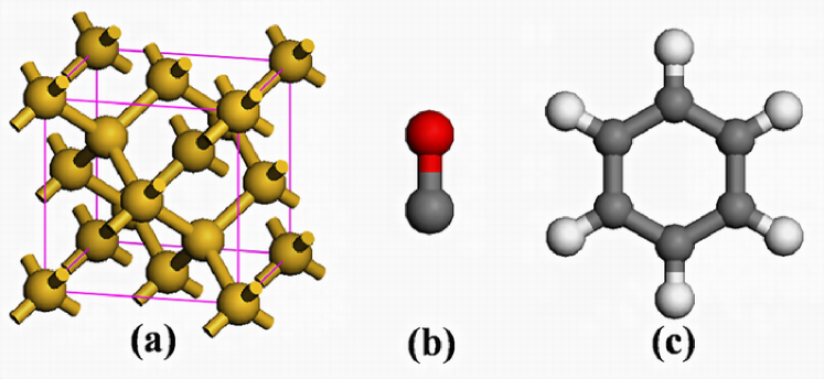
Figure 1: Atomic structures of (a) a bulk silicon Si₈ unit cell, (b) carbon monoxide (CO) and (c) benzene (C₆H₆) molecules. The white, gray, red, and yellow balls denote hydrogen, carbon, oxygen, and silicon atoms, respectively.

7.1 Accuracy

We first measure the accuracy of the ISDF method by comparing the computed eigenvalues of the BSH matrices constructed with and without the ISDF decomposition.

In our test, we set the plane wave energy cutoff required in the QE calculations to $E_{\text{cut}}=10$ Ha, which is relatively low. However, this is sufficient for assessing the effect of ISDF. Such a choice of $E_{\text{cut}}$ results in $N_{r}=35937$ and $N_{g}=2301$ for the Si₈ system, $N_{r}=19683$ and $N_{g}=1237$ for the CO molecule ($N_{v}=5$), $N_{r}=91125$ and $N_{g}=6235$ for the benzene molecule. We only include the lowest $N_{c}$ conducting bands in the BSE calculation. The number of active conduction bands ($N_{c}$) and valence bands ($N_{v}$), the number of reciprocal grids and the dimensions of the corresponding BSE Hamiltonian $H_{\text{BSE}}$ for these three systems are listed in Table 1.

Table 1: Parameters of system size for bulk silicon Si₈, carbon monoxide (CO) and benzene (C₆H₆) molecules used for constructing corresponding BSE Hamiltonian $H_{BSE}$.

System		$N_{r}$		$N_{g}$		$N_{v}$		$N_{c}$		dim($H_{BSE}$)
Si8		35937		2301		16		64		2048
CO		19683		1237		5		60		600
Benzene		91125		6235		15		60		1800

In Fig. 2, we plot the singular values of the matrices $M_{vc}(\mathbf{r})=\{\psi_{i_{c}}(\mathbf{r})\bar{\psi}_{i_{v}}(\mathbf{r})\}$, $M_{cc}(\mathbf{r})=\{\psi_{i_{c}}(\mathbf{r})\bar{\psi}_{j_{c}}(\mathbf{r})\}$ and $M_{vv}(\mathbf{r})=\{\psi_{i_{v}}(\mathbf{r})\bar{\psi}_{j_{v}}(\mathbf{r})\}$ associated with the CO molecule. We observe that the singular values of these matrices decay rapidly. For example, the leading 500 (out of 3600) singular values of $M_{cc}(\mathbf{r})$ decreases rapidly towards zero. All other singular values are below $10^{-4}$. Therefore, the numerical rank $N_{cc}^{t}$ of $M_{cc}$ is roughly 500 ($t$ = 8.3), or roughly 15% of the number of columns in $M_{cc}$. Consequently, we expect that the rank of $\Theta_{cc}$ produced in ISDF decomposition can be set to 15% of $N_{c}^{2}$ without sacrificing the accuracy of the computed eigenvalues.

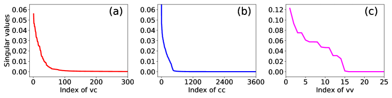
Figure 2: The singular values of (a) $M_{vc}(\mathbf{r})=\{\psi_{i_{c}}(\mathbf{r})\bar{\psi}_{i_{v}}(\mathbf{r})\}$ ($N_{vc}=300$), (b) $M_{cc}(\mathbf{r})=\{\psi_{i_{c}}(\mathbf{r})\bar{\psi}_{j_{c}}(\mathbf{r})\}$ ($N_{cc}=3600$) and (c) $M_{vv}(\mathbf{r})=\{\psi_{i_{v}}(\mathbf{r})\bar{\psi}_{j_{v}}(\mathbf{r})\}$ ($N_{vv}=25$).

This prediction is confirmed in Fig. 3, where we plot the absolute difference between the lowest the exciton energy of Si₈ computed with and without using ISDF to construct $H_{\text{BSE}}$. To be specific, the error in the desired eigenvalue is computed as $\Delta{E}=E_{\text{ISDF}}-E_{\text{BGW}}$, where $E_{\text{ISDF}}$ is computed from the $H_{\rm{BSE}}$ constructed with ISDF approximation, and $E_{\text{BGW}}$ is computed from a standard $H_{\text{BSE}}$ constructed without using ISDF. We first vary one of the ratios $N^{t}_{cc}/N_{cc}$, $N^{t}_{vc}/N_{vc}$ and $N^{t}_{vv}/N_{vv}$ while holding the others at a constant of $1$. We observe that the error in the lowest exciton energy (positive eigenvalue) is around $10^{-3}$ Ha, when either $N^{t}_{cc}/N_{cc}$ or $N^{t}_{vc}/N_{vc}$ is set to 0.1 while the other ratios are held at 1. However, reducing $N^{t}_{vv}/N_{vv}$ to 0.1 introduces a significant amount of error (0.1 Ha) in the lowest exciton energy. This is likely due to the fact that $N_{v}=16$ is too small. We then hold $N^{t}_{vv}/N_{vv}$ at 0.5 and let both $N^{t}_{cc}/N_{cc}$ and $N^{t}_{vc}/N_{vc}$ vary. The variation of $\Delta{E}$ with respect to these ratios is also plotted as in Fig. 3. We observe that the error in the lowest exciton energy is still around $10^{-3}$ Ha even when both $N^{t}_{cc}/N_{cc}$ and $N^{t}_{vc}/N_{vc}$ are set to 0.1.

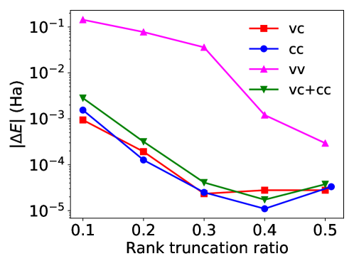
Figure 3: The change of absolute error $\Delta E$ in the smallest eigenvalue of $H_{\text{BSE}}$ associated with the Si₈ system with respect to different truncation levels used in ISDF approximation of $M_{vc}$, $M_{cc}$ and $M_{vv}$. The curves labeled by ‘vc’, ‘cc’, ‘vv’ correspond to calculations in which only one of the ratios $N_{vc}^{t}/N_{vc}$, $N_{cc}^{t}/N_{cc}$ and $N_{vv}^{t}/N_{vv}$ changes while all other parameters are held constant. The curve labeled by ‘vc + cc’ corresponds to the calculation in which both $N_{vc}^{t}/N_{vc}$ and $N_{cc}^{t}/N_{cc}$ change at the same rate ($N_{vv}^{t}=N_{vv}$).

We then check the absolute error $\Delta{E}$ (Ha) of all the exciton energies computed with the ISDF method by comparing them with the ones obtained from a conventional BSE calculation implemented in BerkeleyGW for the CO and benzene molecules. As we can see from Fig. 4, the errors associated with these eigenvalues are all below $0.002$ Ha when $N^{t}_{cc}/N_{cc}$ is $0.1$.

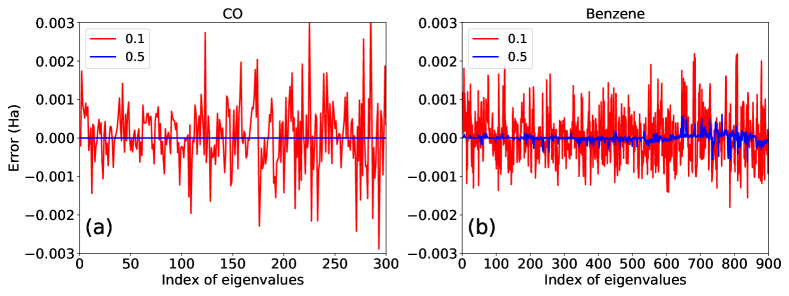
Figure 4: Error in all eigenvalues of the BSH associated with the CO (a) and benzene (b) molecules. Two rank truncation ratios $N^{t}_{cc}/N_{cc}=0.5$ ($t=30.0$) and $N^{t}_{cc}/N_{cc}=0.1$ ($t=6.0$) are used in the tests.

7.2 Efficiency

At the moment, we have only implemented a sequential version of the ISDF method within the BerkeleyGW software package. Therefore, our efficiency test is limited in the size of the problem as well as the number of conducting bands ($N_{c}$) we can include in the bare and screened exchange operators. As a result, our performance measurement does not fully reflect the computational complexity analysis presented in the previous sections. In particular, taking benzene as an example, $N_{g}=6235$ is much larger than $N_{v}=15$ and $N_{c}=60$, therefore the computational cost of $N_{g}^{2}N_{v}^{2}\sim\mathcal{O}(N_{e}^{4})$ term is much higher than the $N_{g}N_{v}^{2}N_{c}^{2}\sim\mathcal{O}(N_{e}^{5})$ term in the conventional BSE calculations.

Nonetheless, in this section, we will demonstrate the benefit of using ISDF to reduce the cost for constructing the BSE Hamiltonian $H_{\text{BSE}}$. In Table 2, we focus on the benzene example and report the wall-clock time required to construct the ISDF approximations of the $M_{vc}$, $M_{cc}$, and $M_{vv}$ matrices at different rank truncation levels. Without using ISDF, it takes 746.0 seconds to construct the reciprocal space representations of $M_{vc}$, $M_{cc}$, and $M_{vv}$ in BerkeleyGW. Most of the timing is spent in the large number of FFTs applied to $M_{vc}$, $M_{cc}$, and $M_{vv}$ to obtain the reciprocal space representation of these matrices. We can clearly see that if only $N^{t}_{cc}/N_{cc}$ is changed from 0.5 ($t$ = 30.0) to 0.1 ($t$ = 6.0), the wall-clock time used to construct a low rank approximation to $M_{cc}$ can be reduced from 578.9 to 34.3 seconds. Furthermore, the total cost of computing $M_{vc}$, $M_{cc}$ and $M_{vv}$ can be further reduced to around 1/19th that in a conventional approach (39.3 vs. 746.0 seconds) if $N^{t}_{vc}/N_{vc}$, $N^{t}_{vv}/N_{vv}$ and $N^{t}_{cc}/N_{cc}$ are all set to 0.1.

Table 2: The variation of time required to carry out the ISDF decomposition of $M_{vc}$, $M_{vv}$ and $M_{cc}$ with respect to rank truncation ratio.

Rank truncation ratio				Time (s) for $M_{ij}(\mathbf{r})$
$N_{vc}^{t}$/$N_{vc}$	$N_{vv}^{t}$/$N_{vv}$	$N_{cc}^{t}$/$N_{cc}$		$M_{vc}$	$M_{vv}$	$M_{cc}$
1.0	0.5	0.5		157.0	5.8	578.9
1.0	0.5	0.1		157.0	5.8	34.3
0.1	0.1	0.1		4.3	0.7	34.3

Note that because ISDF decomposition is carried out on a real space grid, its measured cost reflect the cost for performing QRCP in real space. Even though QRCP with random sampling has $\mathcal{O}(N_{e}^{3})$ complexity, it has a relatively large pre-constant compared to the size of the problem. Hence the measured cost of QRCP is relatively high in this case. Recently, Dong et al. proposed a new approach to find the interpolation points based on the centroidal Voronoi tessellation (CVT) method [6], which offers a much less expensive alternative to the QRCP procedure when the ISDF method is used in hybrid functional calculations. We will explore this CVT method in the BSE-ISDF calculations in the future.

In Table 3, we report the wall-clock time required to construct the projected bare and screened exchange matrices $\widetilde{V}_{A}$ and $\widetilde{W}_{A}$ that appear in Equation (11) once the ISDF approximations of $M_{vc}$, $M_{vv}$, and $M_{cc}$ become available. Without ISDF, it takes $1.574+4.198=5.772$ seconds to construct both $W_{A}$ and $V_{A}$. When $N_{cc}^{t}$/$N_{cc}$ is set to 0.1 only, the construction cost for $W_{A}$, which is the dominant cost, is reduced by a factor of 2.8. Furthermore, if $N^{t}_{vc}/N_{vc}$, $N^{t}_{vv}/N_{vv}$ and $N^{t}_{cc}/N_{cc}$ are all set to 0.1. We reduce the cost for constructing $\widetilde{V}_{A}$ and $\widetilde{W}_{A}$ by a factor of 63.0 and 10.1, respectively. Note that the original implementation of the $W_{A}$ and $V_{A}$ in BerkeleyGW is much slower because the elements of $W_{A}$ and $V_{A}$ are integrated one by one. For benzene, it take takes $103{,}154$ seconds ($28.65$ hours) to construct the BSE Hamiltonian $H_{\text{BSE}}$ in the original BerkeleyGW code.

Table 3: The variation of time required to construct the projected bare and screened exchange matrices $\widetilde{V}_{A}$ and $\widetilde{W}_{A}$ exhibited by the ISDF method respect to rank truncation ratio.

Rank truncation ratio				Time (s) for $H_{\text{BSE}}$
$N_{vc}^{t}$/$N_{vc}$	$N_{vv}^{t}$/$N_{vv}$	$N_{cc}^{t}$/$N_{cc}$		$\widetilde{V}_{A}$	$\widetilde{W}_{A}$
1.0	1.0	1.0		1.574	4.198
1.0	0.5	0.1		1.574	1.474
0.1	0.1	0.1		0.025	0.414

7.3 Optical absorption spectra

One important application of BSE is to compute the optical absorption spectrum, which is determined by optical dielectric function in Equation (14). Fig. 5 plots the optical absorption spectra for both CO and benzene obtained from approximate $H_{\text{BSE}}$ constructed with the ISDF method and the $H_{\text{BSE}}$ constructed in a conventional approach implemented in BerkeleyGW. When the rank truncation ratio $N_{cc}^{t}$/$N_{cc}$ is set to be only 0.10 ($t=6.0$), the absorption spectrum obtained from the ISDF approximate $H_{\text{BSE}}$ is nearly indistinguishable from that produced from the conventional approach. When $N_{cc}^{t}$/$N_{cc}$ is set to 0.05 ($t=3.0$), the absorption spectrum obtained from ISDF approximate $H_{\text{BSE}}$ still preserves the main features (peaks) of the absorption spectrum obtained in a conventional approach even though some of the peaks are slightly shifted, and the height of some peaks are slightly off.

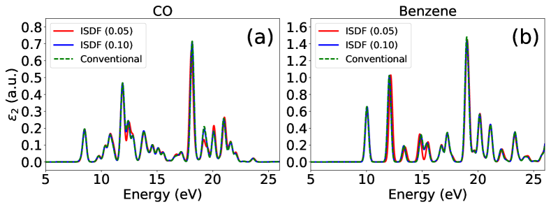
Figure 5: Optical dielectric function (imaginary part $\varepsilon_{2}$) of (a) CO and (b) benzene molecules computed with the ISDF method (the rank ratio $N_{cc}^{t}$/$N_{cc}$ is set to be 0.05 ($t=3.0$) and 0.10 ($t=6.0$)) compared to conventional BSE calculations in BerkeleyGW.

8 Conclusion and outlook

In summary, we have demonstrated that the interpolative separable density fitting (ISDF) technique can be used to efficiently and accurately construct the Bethe–Salpeter Hamiltonian matrix. The ISDF method allows us to reduce the complexity of the Hamiltonian construction from $\mathcal{O}(N_{e}^{5})$ to $\mathcal{O}(N_{e}^{3})$ with a much smaller pre-constant. We show that the ISDF based BSE calculations in molecules and solids can efficiently produce accurate exciton energies and optical absorption spectrum in molecules and solids.

In the future, we plan to replace the costly QRCP procedure with the centroidal Voronoi tessellation (CVT) method [6] for selecting the interpolation points in the ISDF method. The CVT method is expected to significantly reduce the computational cost for selecting interpolating point in the ISDF procedure for the BSE calculations.

The performance results reported here are based on a sequential implementation of the ISDF method. In the near future, we will implement a parallel version suitable for large-scale distributed memory parallel computers. Such an implementation will allow us to tackle much larger problems for which the favorable scaling of the ISDF approach is much more pronounced.

References

- [1] T. Auckenthaler, V. Blum, H. J. Bungartz, T. Huckle, R. Johanni, L. Krämer, B. Lang, H. Lederer, and P. R. Willems. Parallel solution of partial symmetric eigenvalue problems from electronic structure calculations. Parallel Comput., 37(12):783–794, 2011.
- [2] P. Benner, S. Dolgov, V. Khoromskaia, and B. N. Khoromskij. Fast iterative solution of the Bethe–Salpeter eigenvalue problem using low-rank and QTT tensor approximation. J. Comput. Phys., 334:221–239, 2017.
- [3] J. Brabec, L. Lin, M. Shao, N. Govind, Y. Saad, C. Yang, and E. G. Ng. Efficient algorithms for estimating the absorption spectrum within linear response TDDFT. J. Chem. Theory Comput., 11(11):5197–5208, 2015.
- [4] T. F. Chan and P. C. Hansen. Some applications of the rank revealing QR factorization. SIAM J. Sci. Statist. Comput., 13:727–741, 1992.
- [5] J. Deslippe, G. Samsonidze, D. A. Strubbe, M. Jain, M. L. Cohen, and S. G. Louie. BerkeleyGW: A massively parallel computer package for the calculation of the quasiparticle and optical properties of materials and nanostructures. Comput. Phys. Commun., 183(6):1269–1289, 2012.
- [6] K. Dong, W. Hu, and L. Lin. Interpolative separable density fitting through centroidal voronoi tessellation with applications to hybrid functional electronic structure calculations. arXiv:1711.01531, 2017.
- [7] P. Giannozzi, S. Baroni, N. Bonini, M. Calandra, R. Car, C. Cavazzoni, D. Ceresoli, G. L. Chiarotti, M. Cococcioni, I. Dabo, A. D. Corso, S. de Gironcoli, S. Fabris, G. Fratesi, R. Gebauer, U. Gerstmann, C. Gougoussis, A. Kokalj, M. Lazzeri, L. Martin-Samos, N. Marzari, F. Mauri, R. Mazzarello, S. Paolini, A. Pasquarello, L. Paulatto, C. Sbraccia, S. Scandolo, G. Sclauzero, A. P. Seitsonen, A. Smogunov, P. Umari, and R. M. Wentzcovitch. QUANTUM ESPRESSO: A modular and open-source software project for quantum simulations of materials. J. Phys.: Condens. Matter, 21(39):395502, 2009.
- [8] S. Goedecker, M. Teter, and J. Hutter. Separable dual-space Gaussian pseudopotentials. Phys. Rev. B, 54:1703, 1996.
- [9] C. Hartwigsen, S. Goedecker, and J. Hutter. Relativistic separable dual-space gaussian pseudopotentials from H to Rn. Phys. Rev. B, 58:3641, 1998.
- [10] L. Hedin. New method for calculating the one-particle Green’s function with application to the electron–gas problem. Phys. Rev., 139:A796, 1965.
- [11] W. Hu, L. Lin, and C. Yang. Interpolative separable density fitting decomposition for accelerating hybrid density functional calculations with applications to defects in silicon. J. Chem. Theory Comput., 13(11):5420–5431, 2017.
- [12] P. B. V. Khoromskaia and B. N. Khoromskij. A reduced basis approach for calculation of the Bethe CSalpeter excitation energies by using low-rank tensor factorisations. Mol. Phys., 114:1148–1161, 2016.
- [13] A. V. Knyazev. Toward the optimal preconditioned eigensolver: Locally optimal block preconditioned conjugate gradient method. SIAM J. Sci. Comput., 23(2):517–541, 2001.
- [14] C. Lanczos. An iteration method for the solution of the eigenvalue problem of linear differential and integral operators. J. Res. Nat. Bur. Standards, 45:255–282, 1950.
- [15] L. Lin, Z. Xu, and L. Ying. Adaptively compressed polarizability operator for accelerating large scale ab initio phonon calculations. Multiscale Model. Simul., 15:29–55, 2017.
- [16] M. P. Ljungberg, P. Koval, F. Ferrari, D. Foerster, and D. Sánchez-Portal. Cubic-scaling iterative solution of the Bethe–Salpeter equation for finite systems. Phys. Rev. B, 92:075422, 2015.
- [17] J. Lu and K. Thicke. Cubic scaling algorithms for RPA correlation using interpolative separable density fitting. J. Comput. Phys., 351:187–202, 2017.
- [18] J. Lu and L. Ying. Compression of the electron repulsion integral tensor in tensor hypercontraction format with cubic scaling cost. J. Comput. Phys., 302:329–335, 2015.
- [19] M. Marsili, E. Mosconi, F. D. Angelis, and P. Umari. Large-scale GW-BSE calculations with scaling: Excitonic effects in dye-sensitized solar cells. Phys. Rev. B, 95:075415, 2017.
- [20] C. Møler and M. S. Plesset. Note on an approximation treatment for many-electron systems. Phys. Rev., 46:618, 1934.
- [21] G. Onida, L. Reining, and A. Rubio. Electronic excitations: Density-functional versus many-body Green’s-function approaches. Rev. Mod. Phys., 74:601, 2002.
- [22] D. Rocca, D. Lu, and G. Galli. Ab initio calculations of optical absorption spectra: Solution of the Bethe CSalpeter equation within density matrix perturbation theory. J. Chem. Phys., 133:164109, 2010.
- [23] M. Rohlfing and S. G. Louie. Electron–hole excitations and optical spectra from first principles. Phys. Rev. B, 62:4927, 2000.
- [24] E. E. Salpeter and H. A. Bethe. A relativistic equation for bound-state problems. Phys. Rev., 84:1232, 1951.
- [25] M. Shao, F. H. da Jornada, L. Lin, C. Yang, J. Deslippe, and S. G. Louie. A structure preserving Lanczos algorithm for computing the optical absorption spectrum. SIAM J. Matrix. Anal. Appl., to appear.
- [26] M. Shao, F. H. da Jornada, C. Yang, J. Deslippe, and S. G. Louie. Structure preserving parallel algorithms for solving the Bethe CSalpeter eigenvalue problem. Linear Algebra Appl., 488:148–167, 2016.
- [27] M. Shao and C. Yang. BSEPACK user’s guide, 2016. https://sites.google.com/a/lbl.gov/bsepack/.