Variational Formulation for
Wannier functions With Entangled Band Structure

Abstract

Wannier functions provide a localized representation of spectral subspaces of periodic Hamiltonians, and play an important role for interpreting and accelerating Hartree-Fock and Kohn-Sham density functional theory calculations in quantum physics and chemistry. For systems with isolated band structure, the existence of exponentially localized Wannier functions and numerical algorithms for finding them are well studied. In contrast, for systems with entangled band structure, Wannier functions must be generalized to span a subspace larger than the spectral subspace of interest to achieve favorable spatial locality. In this setting, little is known about the theoretical properties of these Wannier functions, and few algorithms can find them robustly. We develop a variational formulation to compute these generalized maximally localized Wannier functions. When paired with an initial guess based on the selected columns of the density matrix (SCDM) method, our method can robustly find Wannier functions for systems with entangled band structure. We formulate the problem as a constrained nonlinear optimization problem, and show how the widely used disentanglement procedure can be interpreted as a splitting method to approximately solve this problem. We demonstrate the performance of our method using real materials including silicon, copper, and aluminum. To examine more precisely the localization properties of Wannier functions, we study the free electron gas in one and two dimensions, where we show that the maximally-localized Wannier functions only decay algebraically. We also explain using a one dimensional example how to modify them to obtain super-algebraic decay.

1 Introduction

Localized representations of electronic wavefunctions have a wide range of applications in quantum physics, chemistry, and materials science. In an effective single particle theory such as Hartree-Fock theory and Kohn-Sham density functional theory (KSDFT) [19, 23], the electronic wavefunctions are characterized by eigenfunctions of single particle Hamiltonian operators. These eigenfunctions generally have significant magnitude in large portions of the computational domain. However, the physically meaningful quantity is not each individual eigenfunction, but the subspace spanned by the collection of a set of eigenfunctions. This is often referred to as the Kohn-Sham subspace, and it is often possible to reduce the computational complexity of various methods by using an alternative, localized representation of the subspace.

Wannier functions provide one such localized representation of the Kohn-Sham subspace. They require significantly less memory to store, and are the foundation of so-called “linear scaling methods” [22, 16, 4] for solving quantum problems. They can also be used to analyze chemical bonding in complex materials, interpolate the band structure of crystals, accelerate ground and excited state electronic structure calculations, and form reduced order models for strongly correlated many body systems [26].

Wannier functions are not uniquely determined, and depend on a choice of gauge (a rotation among the occupied states), which strongly influences their localization. For periodic systems with an isolated band structure, the localization properties of Wannier functions have been studied extensively [21, 3, 31, 5, 35]. Interestingly, the existence of localized Wannier functions in this case is characterized by a topological invariant. For physical systems without magnetic field (invariant under time-reversal symmetry), this topological invariant is trivial, and it is known that there exists a gauge leading to Wannier functions with exponential decay [5, 34]. In this setting, efficient numerical algorithms have been developed to compute these exponentially localized functions [27, 20, 17, 12, 33, 9, 30, 6, 10]. In particular, the widely used maximally-localized Wannier function (MLWF) procedure minimizes the variance (or “spread”) [14, 27] over all possible choices of gauge to obtain localized Wannier functions. In the insulating case, it is known that minimizers of this spread are exponentially localized [35].

The situation becomes significantly more challenging for systems with entangled band structure. Entangled band structure arises in metallic systems, but also in insulating systems when conduction bands or a selected range of bands are to be localized. A straightforward definition of Wannier functions requires the set of all Wannier functions to exactly span the selected spectral subspace. However, such Wannier functions are known to decay slowly in real space. Therefore, the definition of Wannier functions has been generalized to refer to functions spanning a subspace larger than, but containing the given entangled spectral subspace, referred to as a “frozen window” [36]. This is useful for instance in band interpolation, where the additional Wannier functions give rise to extra bands that can simply be ignored. Finding such generalized Wannier functions numerically is considerably more complex, and few algorithms in the literature accomplish this task in a robust fashion. Furthermore, little is known theoretically about the localization properties of the constructed generalized Wannier functions. In order to be consistent with the terminology in the physics literature, we will refer to these generalized Wannier functions simply as Wannier functions, unless otherwise noted.

In this paper, we develop a variational formulation for finding Wannier functions in the entangled setting. We formulate the problem as a nonlinear constrained optimization problem. Practical Wannier function calculations indicate that such nonlinear optimization problems can have many local minima. Hence the solution can strongly depend on the initial guess, and the difficulty of constructing a good initial guess is often a significant impediment to finding Wannier functions in a robust fashion. In order to avoid being trapped at undesirable local minima, we use the recently developed selected columns of the density matrix (SCDM) methodology to construct the initial guess for our variational formulation. This strategy is applicable to both the isolated case [9] and the entangled case [8].

Our variational formulation can be obtained in several theoretically equivalent constructions. We find that one of these formulations yields the so-called partly occupied Wannier functions [37], and can be solved efficiently using standard numerical algorithms for minimization under orthogonality constraints. Our formulation also reveals that the widely used “disentanglement” procedure [36] can be viewed as a splitting method for solving the constrained optimization problem, which only performs a single alternation step between the two pieces of the objective function, and therefore does not achieve a global minimum of the spread. We verify the performance of the variational formulation with real materials such as silicon, copper, and aluminum. In these examples, we find that the fully converged variational formulation consistently provides orbitals with a smaller spread than that from the disentanglement procedure, and is more robust to the choice of initial guess. We also find that the difference between the variational formulation and the disentanglement procedure is often small when used for band structure interpolation.

The variational formulation allows us to study the decay properties of Wannier functions for metallic systems. We present the localization properties of generalized Wannier functions for the free electron gas in one and two dimensions. We find that minimizers of the spread exhibit a weak algebraic decay, related to singularities that we identify in $\mathbf{k}$ space. This slow decay is shown to be not a fundamental property of disentangled Wannier functions, but rather a consequence of the fact that minimizing the spread only imposes finite second moments (or square-integrable first derivatives in $\mathbf{k}$ space). In particular we show in one dimension how to modify the maximally-localized Wannier functions to obtain super-algebraic decay.

The rest of the paper is organized as follows. We first introduce several background topics such as Bloch-Floquet theory, Wannier functions, and the SCDM methodology in section 2. We then present a variational formulation for Wannier functions in section 3, and discuss the relation between our variational formulation and existing methods. Numerical results for real materials and for the free electron gas are given in sections 4 and  5, followed by conclusion and discussion in section 6. Some of the technical details related to the implementation of the variational formulation are given in the Appendix A.

2 Preliminaries

2.1 Bloch-Floquet theory

We first briefly review Bloch-Floquet theory for crystal structures. The Bravais lattice with lattice vectors $\mathbf{a}_{1},\mathbf{a}_{2},\mathbf{a}_{3}\in\mathbb{R}^{3}$ is defined as

$$\mathbb{L}=\left\{\mathbf{R}=\sum_{i=1}^{3}n_{i}\mathbf{a}_{i},\quad n_{1},n_{2},n_{3}\in\mathbb{Z}\right\},$$ (1)

and the lattice vectors define a unit cell in the Bravais lattice

$$\Gamma=\left\{\mathbf{r}=\sum_{i=1}^{3}c_{i}\mathbf{a}_{i}|-1/2\leq c_{1},c_{2},c_{3}<1/2\right\}.$$ (2)

The Bravais lattice induces a reciprocal lattice denoted $\mathbb{L}^{*}$, which is the support of the Fourier transform of $\mathbb{L}$-periodic functions. The lattice vectors of $\mathbb{L}^{*}$ are denoted by $\mathbf{b}_{1},\mathbf{b}_{2},\mathbf{b}_{3}$, with $\mathbf{b}_{i}\cdot\mathbf{a}_{j}=2\pi\delta_{ij}$. A unit cell of the reciprocal lattice is selected and called (with some abuse of language) the Brillouin zone, and is defined as

$$\Gamma^{*}=\left\{\mathbf{k}=\sum_{i=1}^{3}c_{i}\mathbf{b}_{i}|-1/2\leq c_{1},c_{2},c_{3}<1/2\right\}.$$ (3)

For a potential $V$ that is real-valued and $\mathbb{L}$-periodic, i.e.

$$V\left(\mathbf{r}+\mathbf{R}\right)=V(\mathbf{r}),\quad\forall\mathbf{r}\in\mathbb{R}^{3},\mathbf{R}\in\mathbb{L},$$ (4)

we consider the Schrödinger operator in $\mathbb{R}^{3}$

$$\mathcal{H}=-\frac{1}{2}\Delta+V.$$

The Bloch-Floquet theory allows us to relabel the spectrum of $\mathcal{H}$ using two indices $(n,\mathbf{k})$, where $n\in\mathbb{N}$ is the band index, and $\mathbf{k}\in\Gamma^{*}$ is the Brillouin zone index. The generalized (not square-integrable) eigenfunction $\psi_{n,\mathbf{k}}(\mathbf{r})$ is known as a Bloch orbital and satisfies

$$\mathcal{H}\psi_{n,\mathbf{k}}(\mathbf{r})=\varepsilon_{n,\mathbf{k}}\psi_{n,\mathbf{k}}(\mathbf{r}).$$

Importantly, $\psi_{n,\mathbf{k}}$ can be decomposed as

$$\psi_{n,\mathbf{k}}(\mathbf{r})=e^{\imath\mathbf{k}\cdot\mathbf{r}}u_{n,\mathbf{k}}(\mathbf{r}),$$ (5)

where $u_{n,\mathbf{k}}(\mathbf{r})$ is a periodic function with respect to $\mathbb{L}$. Eigenpairs $(\varepsilon_{n,\mathbf{k}},u_{n,\mathbf{k}})$ can therefore be obtained by solving the eigenvalue problem

$$\mathcal{H}(\mathbf{k})u_{n,\mathbf{k}}=\varepsilon_{n,\mathbf{k}}u_{n,\mathbf{k}},\quad n\in\mathbb{N},\quad\mathbf{k}\in\Gamma^{*},$$ (6)

where $\mathcal{H}(\mathbf{k})=\frac{1}{2}(-\imath\nabla+\mathbf{k})^{2}+V(\mathbf{r})$. For each $\mathbf{k}$, the eigenvalues $\varepsilon_{n,\mathbf{k}}$ are ordered non-decreasingly, and $\{\varepsilon_{n,\mathbf{k}}\}$ as a function of $\mathbf{k}$ for a fixed $n$ is called a band. The set of all eigenvalues is called the band structure of the crystal and characterizes the spectrum of the operator $\mathcal{H}$. If $\varepsilon_{N+1,\mathbf{k}}>\varepsilon_{N,\mathbf{k}}$ for all $\mathbf{k}\in\Gamma^{*}$, then the first $N$ bands are isolated. This is for instance the case in the occupied bands of an insulator. When the gap condition $\varepsilon_{N+1,\mathbf{k}}>\varepsilon_{N,\mathbf{k}}$ does not hold, the band structure becomes entangled. Entangled band structure appears not only in metallic systems, but also insulating systems when a Wannier representation of part of the conduction bands is required.

2.2 Wannier functions

For simplicity, we first consider systems with isolated first $N$ bands—an assumption we will drop towards the end of this section. Rotating the set of functions $\{\psi_{n,\mathbf{k}}\}$ by an arbitrary unitary matrix $U(\mathbf{k})\in\mathbb{C}^{N\times N}$, we can define a new set of functions

$$\widetilde{\psi}_{n,\mathbf{k}}(\mathbf{r})=\sum_{m=1}^{N}\psi_{m,\mathbf{k}}(\mathbf{r})U_{m,n}(\mathbf{k}),\quad\mathbf{k}\in\Gamma^{*}.$$ (7)

A given set of of such matrices $\{U(\mathbf{k})\}_{\mathbf{k}\in\Gamma^{*}}$ is called a gauge.

For each $\mathbf{k}$, we consider the density matrix $P(\mathbf{k})$, which is the projector on the the eigenspace corresponding to the first $N$ eigenvalues of $H(\mathbf{k})$

$$P(\mathbf{k})=\sum_{n=1}^{N}\lvert\psi_{n,\mathbf{k}}\rangle\langle\psi_{n,\mathbf{k}}\rvert=\sum_{n=1}^{N}\lvert\widetilde{\psi}_{n,\mathbf{k}}\rangle\langle\widetilde{\psi}_{n,\mathbf{k}}\rvert.$$ (8)

Importantly, for each $\mathbf{k}$, the density matrix $P(\mathbf{k})$ is gauge-invariant. If $\mathcal{C}$ is a contour in the complex plane enclosing the eigenvalues $\varepsilon_{1,\mathbf{k}},\dots,\varepsilon_{N,\mathbf{k}}$ (and only those), then the Cauchy integral formula yields an alternative representation of $P(\mathbf{k})$

$$P(\mathbf{k})=\frac{1}{2\pi\imath}\int_{\mathcal{C}}\frac{1}{\lambda-H(\mathbf{k})}\,\mathrm{d}\lambda.$$ (9)

Since $H(\mathbf{k})$ is analytic, it follows that so is $P(\mathbf{k})$.

Given a choice of gauge, the Wannier functions are defined as [39]

$$w_{n,\mathbf{R}}(\mathbf{r})=\frac{1}{\lvert\Gamma^{*}\rvert}\int_{\Gamma^{*}}\widetilde{\psi}_{n,\mathbf{k}}(\mathbf{r})e^{-\imath\mathbf{k}\cdot\mathbf{R}}\,\mathrm{d}\mathbf{k},\quad\mathbf{r}\in\mathbb{R}^{3},\mathbf{R}\in\mathbb{L},$$ (10)

where $\lvert\Gamma^{*}\rvert$ is the volume of the first Brillouin zone. This represents a unitary transformation from the family $(\psi_{n,\mathbf{k}})_{n=1,\dots,N,\mathbf{k}\in\Gamma^{*}}$ to $(w_{n,\mathbf{R}})_{n=1,\dots,N,\mathbf{R}\in\mathbb{L}}$. In particular, the Wannier functions $w_{n,\mathbf{R}}$ are orthogonal to each other and span the same space as the range of the total density matrix $\frac{1}{|\Gamma^{*}|}\int_{\Gamma^{*}}P(\mathbf{k})\,\mathrm{d}\mathbf{k}$. They are also translation invariant: $w_{n,\mathbf{R}}(\mathbf{r})=w_{n}(\mathbf{r}-\mathbf{R})$.

For insulating systems, in the absence of topological obstructions, there exists a gauge such that $\widetilde{\psi}_{n,\mathbf{k}}$ is analytic and $\mathbb{L}^{*}$-periodic in $\mathbf{k}$, implying that the Fourier transform of $w_{n,\mathbf{R}}$ is analytic, and therefore that each Wannier function decays exponentially as $\lvert\mathbf{r}\rvert\to\infty$ [3, 5, 34]. The Wannier localization problem is reduced to the problem of finding a gauge $\{U(\mathbf{k})\}$ such that $w_{n,\mathbf{0}}$ is localized, or, equivalently, that $\widetilde{\psi}_{n,\mathbf{k}}$ is smooth with respect to $\mathbf{k}$. This can be done by minimizing the “spread functional” [14, 27]

$$\Omega[\{U(\mathbf{k})\}]=\sum_{n=1}^{N}\int\lvert w_{n,\mathbf{0}}(\mathbf{r})\rvert^{2}\mathbf{r}^{2}\,\mathrm{d}\mathbf{r}-\left|\int\lvert w_{n,\mathbf{0}}(\mathbf{r})\rvert^{2}\mathbf{r}\,\mathrm{d}\mathbf{r}\right|^{2}.$$ (11)

Here $w_{n,\mathbf{0}}$ depends on $U(\mathbf{k})$ through $\widetilde{\psi}_{n,\mathbf{k}}$ as in Eq. (10). This problem is usually solved by a minimization algorithm such as steepest descent or conjugate gradient with projections at each step to respect the constraints that $U(\mathbf{k})$ must be unitary [28, 29].

For systems with entangled band structure, the density matrix $P(\mathbf{k})$ as defined in Eq. (8) is no longer smooth with respect to $\mathbf{k}$. As a result, there is no choice of gauge $U(\mathbf{k})$ that leads to a set of rotated Bloch orbitals that is smooth with respect to $\mathbf{k}$, and Wannier functions defined strictly according to Eq. (10) will then decay very slowly in real space [16]. In order to enhance the localization properties of Wannier functions, the definition of Wannier functions has been generalized so that the spectral subspace interest is only a proper subspace of that spanned by Wannier functions [36]. In the physics literature, the spectral subspace is described by a “frozen window” along the energy spectrum, and the Wannier functions are linear combinations of orbitals from a larger set described by an “outer window”.

More specifically, we first fix a number of bands $N_{o}$ that determines the outer window and then proceed to look for Wannier functions built out of $\psi_{1,\mathbf{k}},\dots,\psi_{N_{o},\mathbf{k}}$. Next, for each $\mathbf{k}$ point we fix a set of frozen bands $\mathcal{N}_{f}(\mathbf{k})\subset\left[N_{o}\right],$ and let $N_{f}(\mathbf{k})=\lvert\mathcal{N}_{f}(\mathbf{k})\rvert.$ $\mathcal{N}_{f}(\mathbf{k})$ are often defined as the bands within a fixed energy window that we will try to reproduce. Correspondingly, we define the frozen density matrix as

$$P_{f}(\mathbf{k})=\sum_{n\in\mathcal{N}_{f}(\mathbf{k})}\lvert\psi_{n,\mathbf{k}}\rangle\langle\psi_{n,\mathbf{k}}\rvert,$$ (12)

which is the projection onto the states within the frozen energy window. Again, the frozen density matrix as defined in Eq. (12) is not smooth with respect to $\mathbf{k}$.

We now seek to construct a set of $N_{w}$ Wannier functions that span the subspace defined by the range of $\frac{1}{|\Gamma^{*}|}\int_{\Gamma^{*}}P_{f}(\mathbf{k})\,\mathrm{d}\mathbf{k}$. We introduce the gauge matrices $U(\mathbf{k})\in\mathbb{C}^{N_{o}\times N_{w}}$ with orthonormal columns, with $\left\lvert N_{f}(\mathbf{k})\right\rvert\leq N_{w}\leq N_{o}$, such that

$$\widetilde{\psi}_{n,\mathbf{k}}(\mathbf{r})=\sum_{m=1}^{N_{o}}\psi_{m,\mathbf{k}}(\mathbf{r})U_{m,n}(\mathbf{k}),\quad\mathbf{k}\in\Gamma^{*},n=1,\ldots,N_{w}.$$ (13)

This may equivalently expressed in matrix form as $\widetilde{\Psi}(\mathbf{k})=\Psi(\mathbf{k})U(\mathbf{k})$. This choice of gauge also induces a density matrix of rank $N_{w}$ for each $\mathbf{k}$ defined as

$$P_{w}(\mathbf{k})=\sum_{n=1}^{N_{w}}\lvert\widetilde{\psi}_{n,\mathbf{k}}\rangle\langle\widetilde{\psi}_{n,\mathbf{k}}\rvert=\widetilde{\Psi}(\mathbf{k})\widetilde{\Psi}^{*}(\mathbf{k})=\Psi(\mathbf{k})U(\mathbf{k})U^{*}(\mathbf{k})\Psi^{*}(\mathbf{k}).$$ (14)

Note that unlike the case with isolated band structure where $N_{o}=N_{w},$ here $N_{w}\neq N_{o}$ implies that $U(\mathbf{k})U^{*}(\mathbf{k})\neq I_{N_{o}}.$ Furthermore, since the set of orbitals in the frozen window is only a subset of all possible orbitals, in general the projectors $P_{w}$ and $P_{f}$ do not span the same space. In order to ensure that our Wannier functions span the same subspace as the subspace associated with the frozen window, we require that

$$P_{w}(\mathbf{k})P_{f}(\mathbf{k})=P_{f}(\mathbf{k}),\quad\forall\mathbf{k}\in\Gamma^{*}.$$ (15)

3 Variational formulation for Wannier functions with entangled band structure

We now proceed to develop a variational formulation for Wannier functions. First, we illustrate how to encode the desired constraints when paired with the aforementioned spread functional. Subsequently, to facilitate numerical solution of the optimization problem, we refine how the constraints are expressed. Lastly, we discuss the relation the existing disentanglement procedure to our formulation and discuss how we construct an initial guess using the SCDM methodology.

3.1 Formulating the optimization problem

Without loss of generality, for the following discussion we assume that the frozen orbitals ($\Psi_{f}$) are always ordered before the rest of the orbitals ($\Psi_{r}$). In terms of the notation from the previous section, this means that for each $\mathbf{k}$ the frozen orbitals are represented by the set $\mathcal{N}_{f}(\mathbf{k})=\left\{1,2,\ldots,N_{f}(\mathbf{k})\right\}$ with $N_{f}(\mathbf{k})$ simply representing the number of frozen orbitals per $\mathbf{k}$-point. Now, we may partition the orbitals and the gauge using the following block form

$$\Psi(\mathbf{k})=\begin{bmatrix}\Psi_{f}(\mathbf{k})&\Psi_{r}(\mathbf{k})\end{bmatrix},\quad U(\mathbf{k})=\begin{bmatrix}U_{f}(\mathbf{k})\\ U_{r}(\mathbf{k})\end{bmatrix}.$$ (16)

The matrices $U_{f}(\mathbf{k})$ and $U_{r}(\mathbf{k})$ are of size $N_{f}(\mathbf{k})\times N_{w}$ and $(N_{o}-N_{f}(\mathbf{k}))\times N_{w}$, encoding the weight assigned to the frozen subspace and its complement in the Wannier functions, respectively. The condition that the Wannier functions represent the frozen bands as in Eq. (15) can conveniently be expressed in terms of these matrices as follows.

Proposition 1.

The following statements are equivalent:

1. $P_{w}(\mathbf{k})P_{f}(\mathbf{k})=P_{f}(\mathbf{k})$.

2. $U_{f}(\mathbf{k})U^{*}_{f}(\mathbf{k})=I_{N_{f}(\mathbf{k})}$.

3. $U_{f}(\mathbf{k})U^{*}_{r}(\mathbf{k})=0$ and $U_{f}(\mathbf{k})$ has full row rank.

4. $U(\mathbf{k})=\begin{bmatrix}I_{N_{f}(\mathbf{k})}&0\\ 0&Y(\mathbf{k})\end{bmatrix}X(\mathbf{k})$, where $X(\mathbf{k})$ is a unitary matrix of size $N_{w}\times N_{w}$, and $Y(\mathbf{k})$ is a matrix with orthogonal columns of size $(N_{o}-N_{f}(\mathbf{k}))\times(N_{w}-N_{f}(\mathbf{k}))$.

Proof.

Since each $\mathbf{k}$ point is treated independently, for simplicity we drop the $\mathbf{k}$ dependence in the proof below.

$\mathbf{1\Leftrightarrow 2}:$ From the definition of $P_{w},P_{f}$ we have

$$P_{w}P_{f} =\Psi\begin{bmatrix}U_{f}U_{f}^{*}&U_{f}U_{r}^{*}\\ U_{r}U_{f}^{*}&U_{r}U_{r}^{*}\end{bmatrix}\begin{bmatrix}I&0\\ 0&0\end{bmatrix}\Psi^{*}=\Psi\begin{bmatrix}U_{f}U_{f}^{*}&0\\ U_{r}U_{f}^{*}&0\end{bmatrix}\Psi^{*}$$

$$P_{f} =\Psi\begin{bmatrix}I_{N_{f}}&0\\ 0&0\end{bmatrix}\Psi^{*}$$

The result follows since $\Psi$ has orthogonal columns.

$\mathbf{2\Leftrightarrow 3}:$ From the partition of $U$ we have

$$UU^{*}=\begin{bmatrix}U_{f}U_{f}^{*}&U_{f}U_{r}^{*}\\ U_{r}U_{f}^{*}&U_{r}U_{r}^{*}\end{bmatrix}$$

If $U_{f}U_{f}^{*}=I_{N_{f}}$, since $UU^{*}$ is a projector, it follows that $U_{r}U_{f}^{*}=0$. On the other hand, if $U_{r}U_{f}^{*}=U_{f}U_{r}^{*}=0$, then the fact that $UU^{*}$ is a projector implies that $U_{f}U_{f}^{*}$ is a projector as well. Since it has full row rank, it must therefore be the identity matrix.

$\mathbf{3\Leftrightarrow 4}:$ If 3 is true, then

$$P_{U}=UU^{*}=\begin{bmatrix}I_{N_{f}}&0\\ 0&U_{r}U_{r}^{*}\end{bmatrix}.$$

Then $U_{r}U_{r}^{*}$ is a projector with rank $N_{w}-N_{f}$, or equivalently

$$U_{r}U_{r}^{*}=YY^{*}$$

for some $(N_{o}-N_{f})\times(N_{w}-N_{f})$ matrix $Y$ with orthogonal columns. Then

$$U=P_{U}U=\begin{bmatrix}I_{N_{f}}&0\\ 0&YY^{*}\end{bmatrix}U=\begin{bmatrix}I_{N_{f}}&0\\ 0&Y\end{bmatrix}X,$$

where

$$X=\begin{bmatrix}I_{N_{f}}&0\\ 0&Y^{*}\end{bmatrix}U,$$

and it can be readily verified that $X$ is unitary. The reverse direction is obvious. ∎

Proposition 1 gives us various concise ways to impose the desired condition on the span of Wannier functions, and we may for instance consider using condition $2$. Since the smoothness requirement for $\widetilde{\psi}_{n,\mathbf{k}}$ with respect to the Brillouin zone index $\mathbf{k}$ can be realized by minimizing the spread functional (11), finding the desired smooth gauge $U(\mathbf{k})$ can be recast as the following constrained optimization problem:

$$\begin{split}\inf_{\{U(\mathbf{k})\}}&\quad\Omega[\{U(\mathbf{k})\}]\\ \text{s.t.}&\quad U^{*}(\mathbf{k})U(\mathbf{k})=I_{N_{w}},\quad U_{f}(\mathbf{k})U_{f}^{*}(\mathbf{k})=I_{N_{f}(\mathbf{k})}.\end{split}$$ (17)

The difficulty at this stage is that numerical optimization of (17) with respect to these constraints may not be easy. In particular, the set of matrices $U$ satisfying $U^{*}U=I_{N_{w}}$ and $U_{f}U_{f}^{*}=I_{N_{f}}$ does not necessarily possess a smooth manifold structure. This complicates the application of standard methods for the minimization of functions over orthogonality constraints.

On the other hand, the condition $4$ in Proposition 1 represents $U$ in a factorized form, hereinafter referred to as the $(X,Y)$ representation. This representation of the matrix $U(\mathbf{k})$ gives rise to Wannier functions composed of the $N_{f}(\mathbf{k})$ functions in the frozen window, and another set of $N_{w}-N_{f}(\mathbf{k})$ functions, encoded by the matrix $Y(\mathbf{k})$. This $Y$ encapsulates all the necessary information about the projector $P_{w}=\widetilde{\Psi}\widetilde{\Psi}^{*}$. The unitary $X(\mathbf{k})$ matrix mixes these $N_{w}$ Wannier functions amongst themselves to produce a smooth gauge. In the $(X,Y)$ representation, the variational formulation (17) can be written as

$$\begin{split}\inf_{\{X(\mathbf{k}),Y(\mathbf{k})\}}&\quad\Omega[\{U(\mathbf{k})\}],\\ \text{s.t.}&\quad U(\mathbf{k})=\begin{bmatrix}I_{N_{f}(\mathbf{k})}&0\\ 0&Y(\mathbf{k})\end{bmatrix}X(\mathbf{k}),\\ &\quad X^{*}(\mathbf{k})X(\mathbf{k})=I_{N_{w}},\\ &\quad Y^{*}(\mathbf{k})Y(\mathbf{k})=I_{N_{w}-N_{f}(\mathbf{k})}.\end{split}$$ (18)

This optimization problem is equivalent to the “partly occupied Wannier functions” [37]. This also directly generalizes the maximally localized Wannier functions procedure [27] by Marzari and Vanderbilt for the isolated case.

The $(X,Y)$ representation is a redundant representation, and a given $U$ can be reproduced by many pairs $(X,Y)$. However, in contrast to the formulation (17), the constraint in Eq. (18) defines a Riemannian manifold where $X(\mathbf{k})$ and $Y(\mathbf{k})$ are independent matrices with orthogonality constraints. This allows us to use standard algorithms for the minimization of differentiable functions on Riemannian manifolds to solve the problem. We refer to Appendix A for the details of the computation of the gradient of the objective function $\Omega$.

3.2 Implementation

For our implementation, we modified the Julia [2] library Optim.jl for unconstrained optimization to accommodate constraints represented by Riemannian manifolds [13, 1]. Our modifications have been integrated into that library and are available online . For the numerical tests that follow we used the limited-memory BFGS algorithm [32] with Hager-Zhang line search [18], which gave the best performance compared to other readily-available algorithms (steepest descent, conjugate gradient, BFGS) and line searches (fixed step, backtracking).

In order to generate the initial guess for numerical optimization, we need to convert a given matrix $U$ to a pair $(X,Y)$ that parametrizes it. It will also be useful to consider matrices $U$ that do not satisfy the constraints $U^{*}U=I_{N_{w}}$ and $U_{f}U_{f}^{*}=I_{N_{f}}$ exactly but only approximately. This will allow us to project $U$ to the admissible set that satisfy these constraints.

To find a pair $(X,Y)$ that represents a given $U$, we first choose $Y$ to minimize the error on the projector $UU^{*}$ measured by the Frobenius norm via

$$\inf_{Y^{*}Y=I}\left\|UU^{*}-\begin{bmatrix}I_{N_{f}}&0\\ 0&YY^{*}\end{bmatrix}\right\|_{F}^{2}.$$ (19)

A solution to this problem can be computed using the eigenvalue decomposition

$$U_{r}U_{r}^{*}=VSV^{*}.$$ (20)

When $U$ satisfies the constraints, $U_{r}U_{r}^{*}$ is a projector of rank $N_{w}-N_{f}$, and we can choose $Y$ to be the columns of $V$ corresponding to the $N_{w}-N_{f}$ non-zero eigenvalues of $S$. When $U$ does not satisfy the constraints, we pick $Y$ as the columns of $V$ corresponding to the largest $N_{w}-N_{f}$ eigenvalues of $S$.

Once $Y$ is computed, we can find $X$ that minimizes the error on $U$:

$$\inf_{X^{*}X=I}\left\|U-\begin{bmatrix}I_{N_{f}}&0\\ 0&Y\end{bmatrix}X\right\|_{F}^{2}.$$ (21)

When $U$ satisfies the constraints, the solution of this problem is simply

$$X=\begin{bmatrix}I_{N_{f}}&0\\ 0&Y^{*}\end{bmatrix}U.$$

Otherwise, the solution can again be obtained via the singular value decomposition

$$\begin{bmatrix}I_{N_{f}}&0\\ 0&Y^{*}\end{bmatrix}U=\widetilde{V_{\rm l}}\widetilde{S}\widetilde{V_{\rm r}}^{*},$$ (22)

and setting $X=\widetilde{V_{\rm l}}\widetilde{V_{\rm r}}^{*}$. This step is also called the Löwdin orthogonalization procedure [25].

3.3 Relation to disentanglement

Our variational formulation also gives us a concise way to understand the “disentanglement” procedure of Souza, Marzari and Vanderbilt [36], in which the spread functional is split into two parts

$$\Omega[\{U(\mathbf{k})\}]=\Omega_{I}[\{U(\mathbf{k})\}]+\widetilde{\Omega}[\{U(\mathbf{k})\}].$$ (23)

Here $\Omega_{I}$ is called the gauge-invariant part (depending on $P_{w}$, and hence only on $YY^{*}$), and $\widetilde{\Omega}$ is called the gauge dependent part (depending on $X$). Instead of optimizing (18) directly, [36] proposes to use a two step procedure. First one optimizes the gauge-invariant part only:

$$\inf_{\{Y(\mathbf{k})\}}\quad\Omega_{I}[\{U(\mathbf{k})\}].$$ (24)

This is numerically expedient as $\Omega_{I}$ only depends on $YY^{*}$. In fact, it is analogous to minimization problems in electronic structure (for instance the Hartree-Fock model), where one minimizes the energy, which only depends on the spectral subspace, over all possible orthogonal orbitals. The authors in [36] accordingly obtain a nonlinear eigenvalue problem as the first-order optimality conditions, which they solve using a damped self-consistent field (SCF) iteration.

Once $\{Y(\mathbf{k})\}$ is obtained, it is fixed and so is the projector $P_{w}$. A second minimization problem

$$\inf_{\{X(\mathbf{k})\}}\quad\widetilde{\Omega}[\{U(\mathbf{k})\}]$$ (25)

is then solved with respect to the gauge matrix $X(\mathbf{k})$. This optimization problem is of the same nature as the one for an isolated set of bands.

The total spread from the above two-step procedure is necessarily larger or equal to the global minimum of (18). Interestingly, although the optimal spread can be substantially lower than that found by the two-step disentanglement procedure, numerical experiments show that the quality of Wannier interpolation, measured for instance by the qualify of band structure interpolation, is often similar in both cases.

3.4 Selected column of the density matrix

While the primary purpose of this work is to introduce and analyze a variational formulation of Wannier functions, both the objective function and the constraints are nonlinear, and hence there may exist multiple local minima. It is practically important to seed such methods with a good initial guess. Here, we summarize the recently developed unified methodology for Wannier localization of entangled band structure [8] based on the selected columns of the density matrix (SCDM) methodology [9]. Importantly, this method is direct and robust—no initial guess is required and it will generate valid output—and thus may be reliably used to generate an initial guess.

The SCDM method for entangled band structure first constructs a quasi-density matrix

$$f(H(\mathbf{k}))=\sum_{n=1}^{N_{o}}f\left(\varepsilon_{n,\mathbf{k}}\right)\lvert\psi_{n,\mathbf{k}}\rangle\langle\psi_{n,\mathbf{k}}\rvert,$$ (26)

For insulating systems $f$ would be $1$ on the occupied bands and $0$ otherwise, yielding the projector $P$ as before. For entangled band structure however, the function $f(\cdot)$ is chosen to be large on the bands of interest and decays rapidly, but smoothly, away from them [8]. The SCDM algorithm constructs a gauge by selecting a common set of columns of the $\mathbf{k}$-dependent (quasi-)density matrix $f(H(\mathbf{k}))$. In practice, it is often sufficient to select these columns based on an “anchor” point denoted $\mathbf{k}_{0}$—generically chosen to be the so-called Gamma-point $(0,0,0)^{T}.$

We now briefly outline the SCDM method and refer the reader to [8] for more details. Let $\Psi_{\mathbf{k}}\in\mathbb{C}^{N_{g}\times N_{o}}$ be the matrix with orthogonal columns that represents $\left\{\psi_{n,\mathbf{k}}(\mathbf{r})\right\}$ on a discrete grid in the unit cell, and $\mathcal{E}(\mathbf{k})=\text{diag}\left[\left\{\varepsilon_{n,\mathbf{k}}\right\}_{n=1}^{N_{o}}\right]$ be a diagonal matrix encoding the corresponding eigenvalues. SCDM identifies $N_{w}$ columns of $f(H(\mathbf{k}))$ based on the leading $N_{w}$ columns of the permutation matrix $\Pi$, computed via the QR factorization with column pivoting (QRCP) procedure

$$\Psi_{\mathbf{k}_{0}}^{*}\Pi=QR.$$ (27)

This set of columns is denoted by $\mathcal{C}=\left\{\mathbf{r}_{n}\right\}_{n=1}^{N_{w}}\subset\Gamma$. Now, for each $\mathbf{k}$-point define $\Xi(\mathbf{k})\in\mathbb{C}^{N_{o}\times N_{w}}$ as

$$\Xi_{n,n^{\prime}}(\mathbf{k})=f(\varepsilon_{n,\mathbf{k}})\psi_{n,\mathbf{k}}^{*}(\mathbf{r}_{n^{\prime}}).$$ (28)

It is expected that

$$\widetilde{\psi}_{n,\mathbf{k}}(\mathbf{r})=\sum_{m}\psi_{m,\mathbf{k}}(\mathbf{r})\Xi_{m,n}(\mathbf{k})$$ (29)

is smooth with respect to $\mathbf{k}.$ Therefore, if the singular values of $\Xi(\mathbf{k})$ are uniformly bounded away from 0 in the Brillouin zone, $U(\mathbf{k})$ constructed via Löwdin orthogonalization [25] of $\Xi(\mathbf{k})$ has orthogonal columns, and yields $\left\{\tilde{\psi}_{n,\mathbf{k}}\right\}$ that are smooth with respect to $\mathbf{k}$.

In this framework the frozen bands are not represented exactly, so prior to use in our optimization procedure we must convert from $U$ to a pair $(X,Y)$ via our aforementioned scheme. Since the projector on the frozen set varies discontinuously with $\mathbf{k}$, this procedure does not produce a continuous gauge. However, if the function $f$ is chosen appropriately, it should be close to one. This is further corroborated by the quality of band interpolation, despite the substantially larger spread, we achieve in the numerical results section using the SCDM initial guess without explicitly freezing any bands.

4 Real materials

We first consider the performance of our variational formulation for several real materials. This includes valence and conduction bands of silicon (semiconductor), conduction bands of copper (metal), and valence bands of aluminum (metal). We always start with the aforementioned SCDM based initial guess. We compare the result obtained from the variational formulation to that obtained from the disentanglement procedure in Wannier90, as well as the result obtained directly from the SCDM initial guess without further refinement.

In these experiments, the choice of the parameters of the SCDM procedure are chosen to yield good baseline band structure interpolation. However, they are not “optimized” to minimize band structure interpolation error. These experiments often show how the two optimization methods are comparable, though in some situations we are able to find Wannier functions with smaller spreads using our variational method even given the same initial guess. One interesting point that we will see play out throughout our examples is that the value of the spread and band interpolation quality may not be directly connected, i.e. Wannier functions with considerably different values of spread can yield qualitatively similar interpolation error.

All of the $\mathbf{k}$-point calculations and reference band structure calculations were performed with Quantum ESPRESSO [15]. The SCDM initial guess was constructed using the code available online. Our new variational formulation was implemented in the Julia language and is available online.

4.1 Silicon

Here, we compute the lowest 16 bands of Silicon on an $8\times 8\times 8$ $\mathbf{k}$-point grid and then proceed to compute eight Wannier functions. This includes the four valence bands and four additional low lying conduction bands. For the SCDM procedure we use $\mu=11.0$ and $\sigma=2.0$ with $f$ corresponding to “entangled case 1” in [8]—a complementary error function. For Wannier90 and our method, we freeze bands below 12 eV and set the outer window maximum at infinity. For Wannier90 the prescribed convergence criteria of $1\times 10^{-10}$ on the spread was reached after 225 disentanglement iterations and 95 spread reduction iterations, and for our method after 149 iterations.

Figure 1 shows the band structure interpolation using the three methods. We see that for the four valence bands all three methods perform very well. Furthermore, while there are differences in the interpolation of the conduction bands, no one method clearly outperforms the others. As expected, if we consider the total spread (see Table 1) of the final localized orbitals, our variational formulation yields the most compact orbitals.

In Table 2 we report the per orbital spread for each method, and observe that to the number of significant digits reported all the orbitals found by our method have the same spread (they do not vary until the fourth decimal place). In contrast, Wannier90 seems to converge to two distinct sets of orbitals with slightly different spreads. In Figure 2, we illustrate the differences between the orbitals found with our variational method and those found via Wannier90. We observe that the orbitals obtained from our variational formulation resemble more closely to sp³ hybridized orbitals centering around each Si atom, as indicated from chemical intuition. Interestingly, by using the output of our variational method as input to Wannier90 we are able to force Wannier90 to converge to the same point as our method. Unfortunately, it is difficult to pinpoint a specific cause for the apparent convergence of Wannier90 to a worse local minimum in this setting.

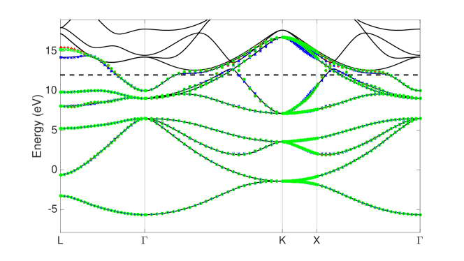
Fig. 1: Wannier interpolation of Silicon with 8 k-points using (blue Xs) SCDM, (green circles) our variational formulation, and (red +s) Wannier90 compared with a (black line) reference calculation. The frozen window is the region below the dotted black line.

Table 1: Silicon spread and valence band error comparison

	Final spread $\left(\text{\AA}^{2}\right)$	max error (eV)	RMSE (eV)
Variational	25.177	0.069	0.021
Wannier90	27.00	0.083	0.023
SCDM	45.206	0.112	0.029

Table 2: Spreads of the eight individual Wannier functions for silicon

	Orbital spread $\left(\text{\AA}^{2}\right)$
Variational	3.15	3.15	3.15	3.15	3.15	3.15	3.15	3.15
Wannier90	3.16	3.16	3.16	3.16	3.59	3.59	3.59	3.59
SCDM	4.93	4.93	4.93	4.93	6.37	6.37	6.37	6.37

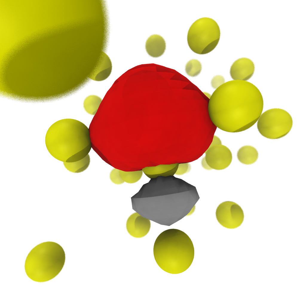
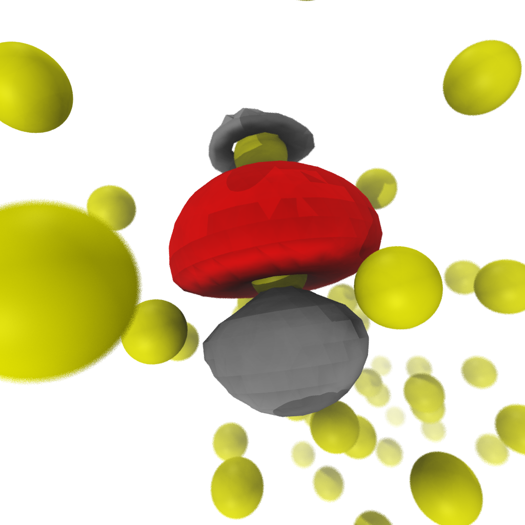
Fig. 2: Example orbitals from our variational method (left) and Wannier90 (right). Here the red and gray isosurfaces are plotted at values $\pm 0.5$ for both normalized orbitals. All of the orbitals we find with our variational method seem to clearly have sp³ hybrid character, as seen in the left figure. In contrast, as illustrated on the right, some of the orbitals found by Wannier90 with larger spread do not share this behavior as clearly.

4.2 Aluminum

We now repeat the same experiments as before, but for the valence bands of the aluminum system with an $8\times 8\times 8$ $\mathbf{k}$-point grid. Specifically, we start with six bands and seek four Wannier functions. For the SCDM procedure we use $\mu=8.42$ and $\sigma=4.0$ with $f$ corresponding to “entangled case 1” in [8]—a complementary error function. Once again, Wannier90 was run until convergence at $10^{-10}$ for both the disentanglement and spread minimization, and reached that threshold after 2,437 and 91 iterations. Our method converged to a spread reduction tolerance of $10^{-10}$ after 138 iterations. As we observe in Figure 3, all three methods once again perform well—particularly below the Fermi energy. The final spreads for each of the three methods are reported in Table 3 along with the spreads of each orbital. While both Wannier90 and our method improve upon the spread of the SCDM initial guess, we do find slightly smaller spread with our optimization procedure. Here, bands below 11.6 eV were frozen in both Wannier90 and our method, and the outer window was set to $\infty.$

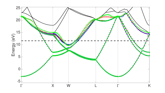
Fig. 3: Wannier interpolation of Aluminum with 8 $\mathbf{k}$-points per direction using (blue Xs) SCDM, (green circles) our variational formulation, and (red +s) Wannier90 compared with a (black line) reference calculation. The frozen window is the region below the dotted black line.

	Orbital spread $\left(\text{\AA}^{2}\right)$				Final spread $\left(\text{\AA}^{2}\right)$
Variational	2.01	2.02	2.02	2.03	8.07
Wannier90	2.09	2.1	2.11	2.11	8.41
SCDM	3.44	4.02	4.21	4.21	15.89

Table 3: Spreads of the four individual Wannier functions for Aluminum and the final spread

We also consider the convergence of the band interpolation error in this setting, looking at both maximum error and RMSE. As before, for both our method and Wannier90 we freeze bands below 11.6 eV and set the outer window to infinity. For all three methods we then measure the error of band interpolation at or below the Fermi energy (8.42 eV). In all cases, we capped Wannier90 at 5,000 disentanglement and spread reduction iterations and considered it converged at a tolerance of $10^{-10}.$ Similarly, we considered our method converged the objective function changed by less than $10^{-10}$ between successive iterates, or we reached 5,000 iterations. Typically our method took 100-250 iterations to converge, whereas the Wannier90 disentanglement would hit the iteration cap and spread reduction took 90-400 iterations to converge. Figure 4 shows broadly similar behavior for all three methods, though generally the two optimization methods do noticeably improve on the SCDM initial guess as more $\mathbf{k}$-points are used. We expect that asymptotically the optimization based methods should perform better. However, given the relatively small number of grid points per direction and the complexity of the band structure, it seems we are still in the pre-asymptotic regime.

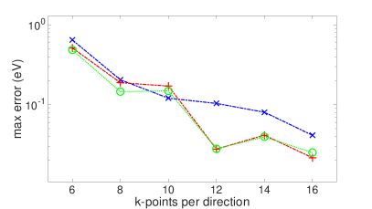
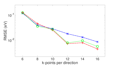
Fig. 4: Max and RMSE in band interpolation for aluminum as computed using (blue Xs) SCDM, (green circles) our variational formulation, and (red +s) Wannier90.

4.3 Copper

Lastly, we illustrate the behavior of our method when used to interpolate seven conduction bands of copper around the Fermi energy. Because several bands that we do not wish to track cross through the energy window, it is not easy to simply look at band interpolation error. Rather, we place emphasis on the qualitative behavior of the interpolation and the orbital spread yielded by our variational formulation. Interestingly, in this case we observed a high sensitivity of Wannier90 to the SCDM initial guess based on the parameters (corresponding to “entangled case 2” in [8]—a Gaussian) and a contrasting robustness of our variational method. In all cases we used a frozen window of 13.5 to 17 eV and no outer window for both Wannier90 and our variational method.

When fixing the parameter $\mu=15.5$ and varying $\sigma$ from $3.0$ to $6.0$, both SCDM and our variational method robustly generated good band interpolation. However, for a range of $\sigma$ Wannier90 with disentanglement failed to reach convergence. To sweep over several values of $\sigma$ we limit Wannier90 to 5,000 iterations each for the disentanglement and spread minimization, and we limit our variational method to 1,000 iterations.

Remark 1.

For $\sigma=5.0$ where we observed particularly bad performance of Wannier90 (see below), we let it run for 100,000 iterations of each the disentanglement and spread. While the disentanglement procedure converged after roughly 20,000 iterations, the spread minimization failed to converge even after 100,000 iterations. While this does not guarantee that the local minimum Wannier90 may eventually find is poor and could simply be the optimization algorithm behaving poorly, we feel this is a reasonable comparison to make even without Wannier90 determining that it has converged. Interestingly, passing the output of Wannier90 in this setting to our variational method we were able to converge to a good gauge.

Figures 5 and 6 show the band interpolation of the three methods in the case where $\sigma=4.0$ and $\sigma=5.0$. We also report the individual spreads of the orbitals in Tables 4 and 5. We observe that in both cases the SCDM initial guess and our optimized solution yield good band interpolation within the frozen window. In contrast, Wannier90 does not find a good local optima in the latter case and this results in poor interpolation quality. We further investigate this behavior in Table 6, where we report the total final spread of the methods as we vary $\sigma$. We see that for two of the parameter values Wannier90 failed to find a local optimum that is close to what our variational method finds.

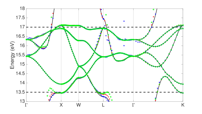
Fig. 5: Using an SCDM initial guess with $\mu=15.5$ and $\sigma=4.0$, Wannier interpolation of copper with 10 k-points using (blue Xs) SCDM, (green circles) our variational formulation, and (red +s) Wannier90 compared with a (black line) reference calculation. The frozen window is the region between the dotted black line.

	Orbital spread $\left(\text{\AA}^{2}\right)$
Variational	0.24	0.50	0.50	0.51	0.56	0.56	1.30
Wannier90	0.41	0.43	0.43	0.48	0.54	0.56	1.41
SCDM	1.49	2.34	2.46	3.06	3.13	3.68	7.50

Table 4: Spreads of the seven individual Wannier functions for copper with the $\sigma=4.0$ initial guess.

	Orbital spread $\left(\text{\AA}^{2}\right)$
Variational	0.21	0.47	0.51	0.52	0.53	0.62	1.38
Wannier90	0.47	0.53	0.54	0.60	0.71	2.78	2.83
SCDM	1.21	1.47	1.56	1.78	1.97	2.53	8.87

Table 5: Spreads of the seven individual Wannier functions for copper with the $\sigma=5.0$ initial guess.

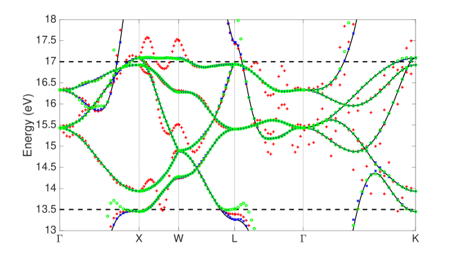
Fig. 6: Using an SCDM initial guess with $\mu=15.5$ and $\sigma=5.0$, Wannier interpolation of Copper with 10 k-points using (blue Xs) SCDM, (green circles) our variational formulation, and (red +s) Wannier90 compared with a (black line) reference calculation. The frozen window is the region between the dotted black line.

$\sigma$	3.0	3.5	4.0	4.5	5.0	5.5	6.0
SCDM	34.22	26.9	23.65	20.83	19.39	18.7	17.3
Our method	4.23	4.17	4.18	4.23	4.23	4.18	4.18
Wannier90	4.27	4.26	4.26	8.48	8.46	4.26	4.26

Table 6: Comparison of the spreads $\left(\text{\AA}^{2}\right)$ for copper as the $\sigma$ parameter of the SCDM initial guess is varied.

5 Free electron gas

We now investigate the decay property of the generalized Wannier functions in real space. This is hard to investigate numerically for real materials because of the very large number of $\mathbf{k}$ points needed to see the asymptotic decay, as evidenced in the previous section. For instance, in [40] the authors report a fast (consistent with exponential) decay up to grid sizes of $15\times 15\times 15$, although the convergence appears to slow down after that. Another problem is that it is hard to find realistic systems in one or two dimensions on which disentangled Wannier systems make sense. The free electron gas, i.e. $V=0$, is explicitly solvable and poses a very interesting benchmark for disentanglement, even in one or two dimensions. In this section, we therefore apply the methodology of Section 3 to $d$-dimensional free electron gas. We simply define the lattice as $\mathbb{L}=2\pi\mathbb{Z}^{d}$, so that $\mathbb{L}^{*}=\mathbb{Z}^{d}$, and we let the Brillouin zone be the set $[0,1)^{d}$.

In this case the eigenfunctions of the operator $H(\mathbf{k})=(-\imath\nabla+\mathbf{k})^{2}$ are given by

$$v_{\mathbf{K}}(\mathbf{r}) =\frac{1}{\sqrt{|\Gamma|}}e^{\imath\mathbf{K}\cdot\mathbf{r}}$$

for $\mathbf{K}$ in the reciprocal lattice $\mathbb{Z}^{d}$. The corresponding eigenvalues are $\varepsilon_{\mathbf{K},\mathbf{k}}=|\mathbf{K}+\mathbf{k}|^{2}$. Notice that since $\varepsilon_{\mathbf{K},\mathbf{k}}$ is the squared distance from $\mathbf{k}$ to $-\mathbf{K}$, the dispersion relation is the set of squared distances of $\mathbf{k}$ to the points of the reciprocal lattice $\mathbb{Z}^{d}$.

We order the eigenfunctions by ordering the eigenvalues in a non-decreasing order. We let $u_{n,\mathbf{k}}=e_{\mathbf{K}_{n}}$, where $\varepsilon_{\mathbf{K}_{n},\mathbf{k}}$ is the $n$-th eigenvalue of $H(\mathbf{k})$, this choice being arbitrary in the presence of degeneracies. The matrix elements $M_{mn}^{\mathbf{k},\mathbf{b}}=\langle u_{m,\mathbf{k}},u_{n,\mathbf{k}+\mathbf{b}}\rangle$ of overlap between neighboring $\mathbf{k}$ points used in the optimization process [27] then assume a particularly simple expression: $M_{mn}^{\mathbf{k},\mathbf{b}}=1$ if $u_{m\mathbf{k}}$ and $u_{n,\mathbf{k}+\mathbf{b}}$ are associated with the same $\mathbf{K}$, and $M_{mn}^{\mathbf{k},\mathbf{b}}=0$ otherwise. In particular, this matrix differs from the identity (it is a permutation matrix) near eigenvalue crossings, where $\varepsilon_{\mathbf{K},\mathbf{k}}=\varepsilon_{\mathbf{K}^{\prime},\mathbf{k}}$ with $\mathbf{K}^{\prime}\neq\mathbf{K}$.

The free electron gas also makes it particularly easy to compute the Wannier functions through their Fourier transforms. For a Wannier function given in $\mathbf{k}$-space by

$$\widetilde{\psi}_{n\mathbf{k}}(\mathbf{r})=\sum_{n\in\mathbb{N}}e^{\imath\mathbf{k}\cdot\mathbf{r}}v_{\mathbf{K}_{m}}(\mathbf{r})U_{mn}(\mathbf{k}),$$

it holds that

$$w_{n,\mathbf{0}}(\mathbf{r})=\int_{[0,1]^{d}}\widetilde{\psi}_{n\mathbf{k}}(\mathbf{r})\,\mathrm{d}\mathbf{k}=\frac{1}{(2\pi)^{d}}\int_{[0,1]^{d}}\sum_{m\in\mathbb{N}}U_{mn}(\mathbf{k})e^{\imath(\mathbf{k}+\mathbf{K}_{m})\cdot\mathbf{r}},$$

from which it follows that $U_{mn}(\mathbf{k})$ is simply the Fourier transform of $w_{n,\mathbf{0}}$ at frequency $\mathbf{\xi}=\mathbf{K}_{m}+\mathbf{k}$.

Note that the free electron gas possesses a large number of symmetries. As a consequence, it has a number of properties that are not expected from generic systems. For instance, eigenvalue crossings are numerous (of co-dimension 1, i.e. points in 1D, lines in 2D and planes in 3D), while they are expected from the von Neumann-Wigner theorem [38] to be rare. This theorem predicts that, in the absence of particular symmetries, the crossing of eigenvalues of a Hermitian matrix are a phenomenon of codimension 3. This is believed to be true (although unproved in many cases) for “generic” Schrödinger operators [24]: for a generic $V$, the band structure is only expected to show crossings in codimension $3$ (isolated points in 3D, and no crossings in lower dimensions). The free electron gas, possessing all the symmetries a Schrödinger operator can have, may thus be considered a worst case system for disentanglement.

5.1 The 1D case

5.1.1 One frozen band, two Wannier functions

The dispersion relation of the 1D free electron gas results in a crossing between the first and second eigenvalues at half-integers and between the second and third eigenvalues at integers (see Figure 7). Because of the crossing between the first and second band, any single Wannier function representing the first band has a maximal decay of $1/r$. We therefore consider the problem of finding two Wannier functions representing the first band ($N_{w}=2,N_{f}=1$). We do not set an outer window but discretize the band structure using $2L+1$ Fourier modes with $L=10$ (as we will see, the Wannier functions we find are compactly supported in Fourier space, and therefore do not depend on the choice of $L\geq 2$).

For this simple system, initializing the gauge randomly allows our optimization algorithm to converge robustly to the same Wannier functions, up to a change of sign and a shift by a lattice vector. It would therefore seem that the global minimizer of the spread is unique (up to the invariant degrees of freedom described above) and real. The SCDM algorithm with the settings $\mu=0$ and $\sigma=2$ yields Wannier functions that are visually indistinguishable from the optimized Wannier functions, and have a very similar spread ($2.51$ for the SCDM algorithm as compared to $2.44$ for the optimized Wannier functions).

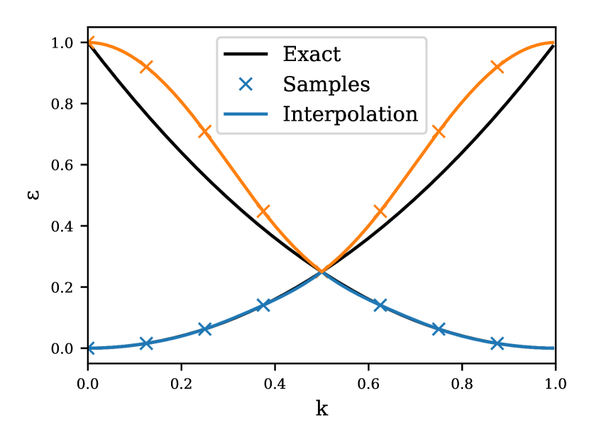
(a) Exact band plot, samples on the $k$-space grid, and Wannier interpolation using the optimized Wannier functions.

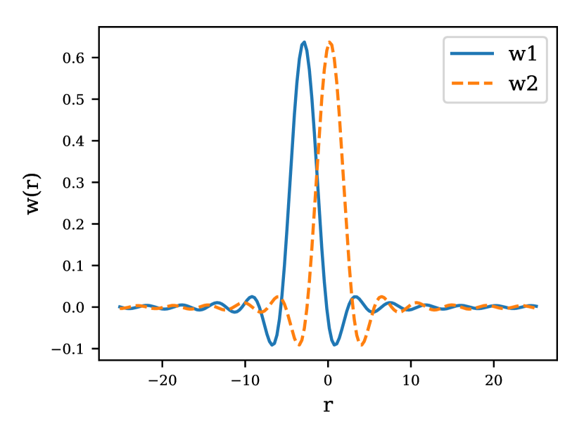
(b) Wannier functions in real space.

Fig. 7: Optimized Wannier functions obtained on a $k$-space grid of size $N=8$.

In Figure 7 we observe that the first band (which is frozen) is exactly reproduced. Since the Wannier functions are localized, the Wannier interpolation is very good, and in particular has no trouble reproducing the crossing. Furthermore, the optimized Wannier functions are symmetric (they are real, and the second one is a translate of the first by half a lattice vector).

However, closer inspection reveals that the optimized Wannier functions are not exponentially localized, and in fact decay as $1/r^{2}$ for large $r$ (Figure 8(b)). The origin of this slow decay of the Wannier functions is the kink that appears at $\xi=\pm 3/2$ in their Fourier transform as in Figure 8(a), which also shows that the Wannier functions are compactly supported on $[-3/2,3/2]$ in Fourier space. This is because only the first three bands are occupied by the Wannier functions, as can be seen via inspection of the $U$ matrix. Since band $3$ crosses with band $4$ at $k=1/2$ (corresponding to basis functions $K=1$ and $K=-2$), the continuity of $\widetilde{\psi}_{nk}$ with respect to $k$ means that $U_{31}(1/2)=U_{32}(1/2)=0$. But the first derivative is not zero at $1/2$, which in turns creates the kink in Fourier space at $K=1,k=1/2$ and $K=-2,k=1/2$, that is, $\xi=\pm 3/2$.

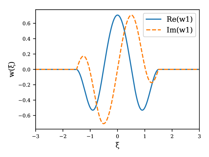
(a) $w_{1}$ in Fourier space: a clear kink is visible at $\xi=\pm 3/2$

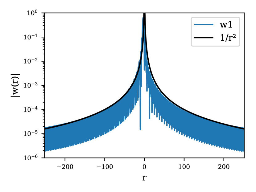
(b) $w_{1}$ in real space, showing excellent agreement with a decay rate $r^{-2}$.

Fig. 8: Optimized Wannier functions obtained on a $k$-space grid of size $N=80$. The kink in Fourier space at $\xi=\pm 3/2$ translates to a $r^{-2}$ decay (only $w_{1}$ represented for clarity). The maximum reconstruction error on the first band is $3\times 10^{-5}$.

The fact that the optimized Wannier functions are only weakly localized is surprising at first glance, because it was proven in [35] that, for isolated bands, maximally-localized Wannier functions are exponentially localized. What is different in this case? The crucial point in the analysis of [35] is that the spread is similar to a Dirichlet energy, or a $H^{1}$ norm, in $k$ space. Then the $\widetilde{\psi}_{nk}$ are shown to satisfy an elliptic equation in $k$ space, which by a bootstrap argument implies their analyticity. Here, this argument breaks down because the constraint $P_{w}(k)P_{f}(k)=P_{f}(k)$ is discontinuous at crossings. This creates an effective “boundary condition” for the gauge $U(k)$ at crossings that destroys the regularity. A simple analogy is that eigenfunctions of the Laplacian on $[0,1]$ (critical points of the Dirichlet energy) are smooth on $\mathbb{R}$ when periodic boundary conditions are imposed, but generically produce kinks at $0$ and $1$ when Dirichlet boundary conditions are imposed. Here also, the effective boundary condition $U_{31}(1/2)=U_{32}(1/2)=0$ produces a kink.

To remedy this, we show on this particular example how to build Wannier functions that are of class $C^{\infty}$ in Fourier space (and therefore decay faster than any inverse polynomial in real space). In order to do so, we define the function $\alpha(x)=e^{-1/x}$ for $x\geq 0$, $\alpha(x)=0$ for $x<0$. This function is $C^{\infty}$, and identically zero for $x\leq 0$. The function $f(x)=\frac{\alpha(x)}{\alpha(x)+\alpha(1-x)}$ is therefore $C^{\infty}$ on $\mathbb{R}$, equal to $0$ for $x\leq 0$, and equal to $1$ for $x\geq 1$.

Given $U(0^{+}),U(1/2^{\pm}),U(1^{-})$ obtained from the optimized Wannier functions, we construct a new gauge

$$\widetilde{U}(k)=\begin{cases}(1-f(2k))U(0^{+})+f(2k)U(1/2^{-})&\text{ if $0<k\leq 1/2$,}\\ (1-f(2k-1))U(1/2^{+})+f(2k-1)U(1^{-})&\text{ if $1/2<k<1$.}\end{cases}$$

This produces a new set of $\widetilde{\psi}_{nk}$ that are smooth with respect to $k$, but not orthogonal and do not span the frozen bands. We now impose those conditions in the same way we do for the SCDM procedure as described in Section 3.4. In this specific example, this produces a smooth gauge, as illustrated in Figure 9.

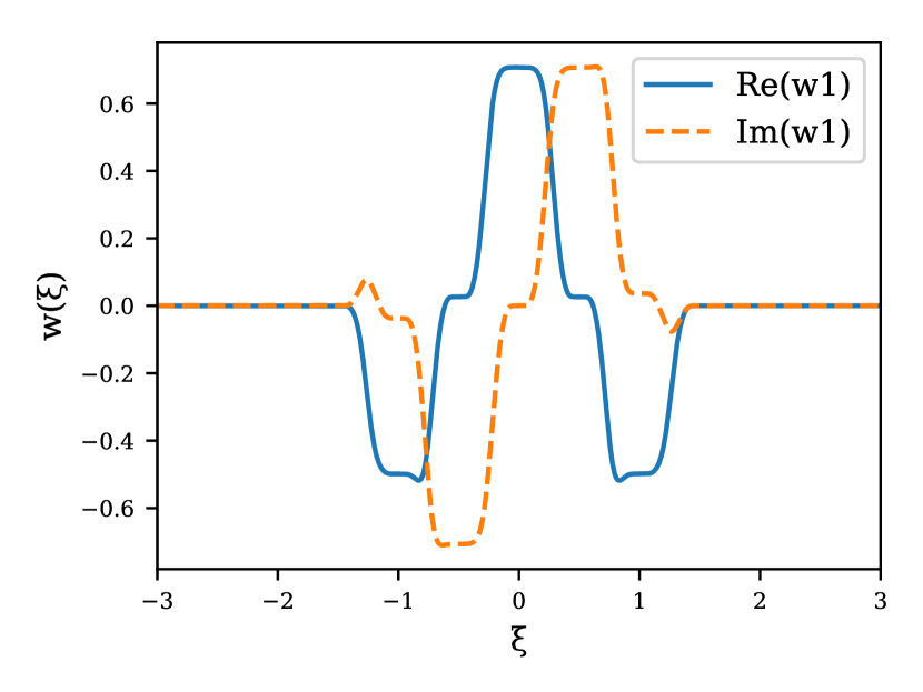
(a) Smoothed Wannier function in Fourier space: although the variations are more rugged than Figure 8, it is a $C^{\infty}$ function.

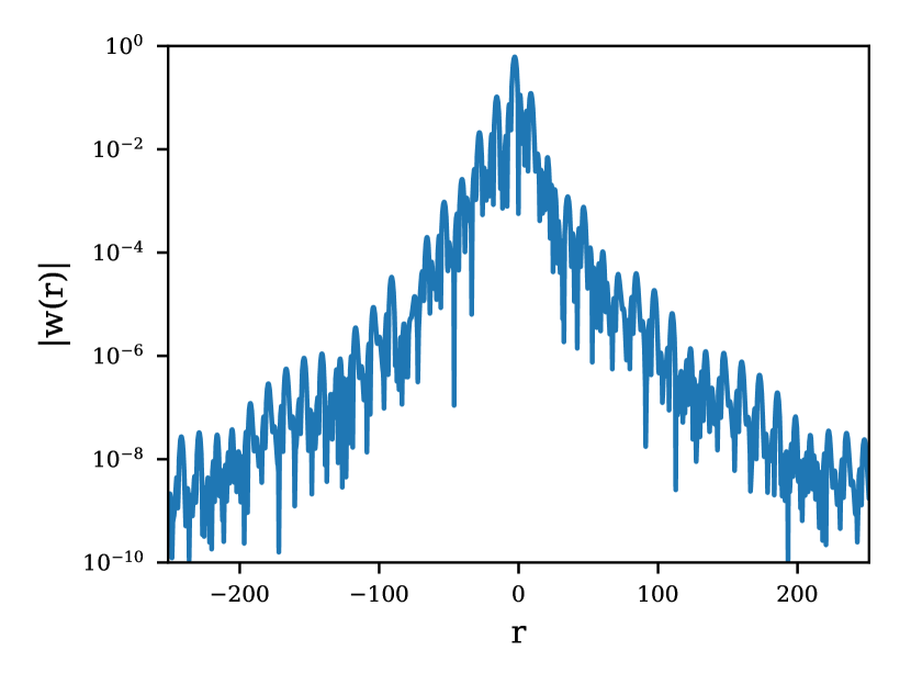
(b) Smoothed Wannier function in real space: the asymptotic decay is much faster than in Figure 8.

Fig. 9: Smoothed Wannier functions obtained on a $k$-space grid of size $N=80$ (see main text for details, only the first Wannier function represented for clarity). The maximum reconstruction error on the first band is $2\times 10^{-9}$.

The Wannier functions obtained in this way display more rugged variation in Fourier space (a consequence of the use of the function $f$ above), and accordingly the decay is slower for small values of $x$. However, because the gauge is smooth, the Wannier functions decay much faster for large values. Since the gauge is of class $C^{\infty}$ but not analytic, the Wannier functions decay faster than any polynomial, but not exponentially. Since the error of Wannier interpolation on the first band is determined by the interaction of the Wannier functions on the supercell with their periodic images, the faster asymptotic decay leads to a better reconstruction of the first band in this case. Numerical tests indicate that the cross-over point (above which the reconstruction error on the first band with the smoothing procedure is smaller than that with the optimized Wannier functions) is around $N=12$.

5.1.2 General case in 1D

In the one-dimensional free electron gas crossings only happen at half-integers, and between two bands at the same time. Accordingly, whenever $N_{w}\geq N_{f}+1$ we can construct optimized Wannier functions similar to the ones above—they are translates of each other, compactly supported in Fourier space, and decay as $1/r^{2}$. When $N_{w}=N_{f}$ (that is, we are treating a metal as if it was an insulator), the gauge is discontinuous, and the corresponding Wannier functions decay as $1/r$.

5.2 The 2D case

In 2D, the first four bands of the free electron gas are degenerate at $\mathbf{k}=(1/2,1/2)$, corresponding to the wave vectors

$$\mathbf{K}=(0,0),(-1,0),(0,-1),(-1,-1).$$

This means that $P_{w}(1/2,1/2)$ must span the four-dimensional subspace corresponding to those four wave vectors. Therefore, freezing the first band can only produce localized Wannier functions when $N_{w}\geq 4$. Accordingly, we consider the case $N_{f}=1$ and $N_{w}=4.$

Similarly to the 1D case, the optimized Wannier functions are real, and differ from each other only by a change of origin. However, they are not compactly supported in Fourier space, and instead have decaying components on arbitrarily large wave vectors $\mathbf{K}$ (see Figure 10(a)). Their support in Fourier space displays a checkerboard pattern, and in particular has corners. Furthermore, we observe numerically that the gradient in Fourier space blows up near those corners when the size of the $k$-point grid $N$ is increased (see Figure 10(b)). The maximum value of the gradient is found to behave as $N^{1/3}$. This is consistent with the singularity of the first eigenfunction of the Laplace operator with Dirichlet boundary conditions on a domain with corners, which behave as $r^{2/3}\sin(2\theta/3)$ near a corner described by $\theta\in[0,3\pi/2]$ in polar coordinates [11]. In particular, their gradient behaves as $r^{-1/3}$ near the corner, explaining the divergence as $N^{1/3}$ when discretized on a grid. As in the 1D case, imposing frozen bands acts as an effective boundary condition for the gauge and destroys the regularity.

The decay of the optimized Wannier functions in Fourier space is dictated by the singularity in Fourier space. More precisely, the first derivative is discontinuous along edges, which corresponds to a decay of the Wannier functions in the $x$ and $y$ directions as $1/r^{2}$.

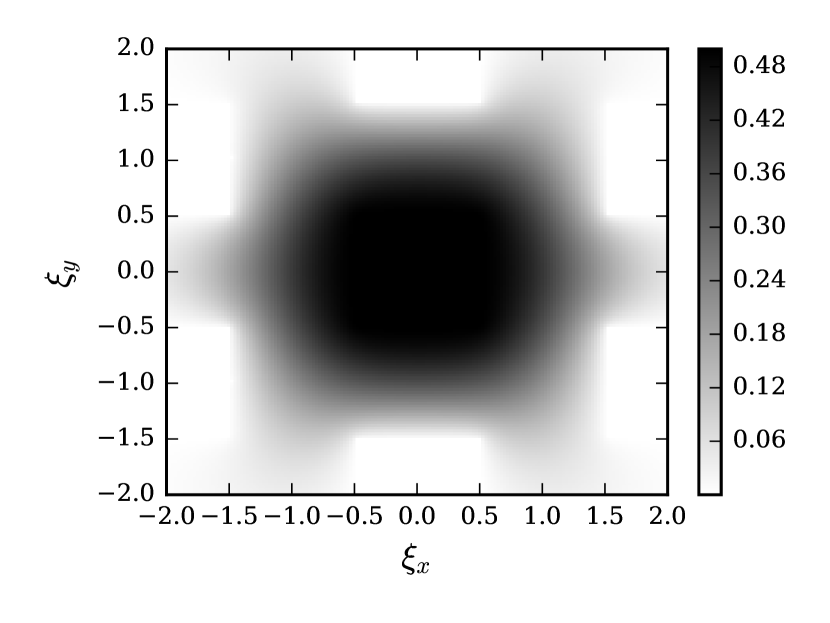
(a) $|\widehat{w}_{2}(\xi)|$. The function has components on arbitrarily large wave vectors.

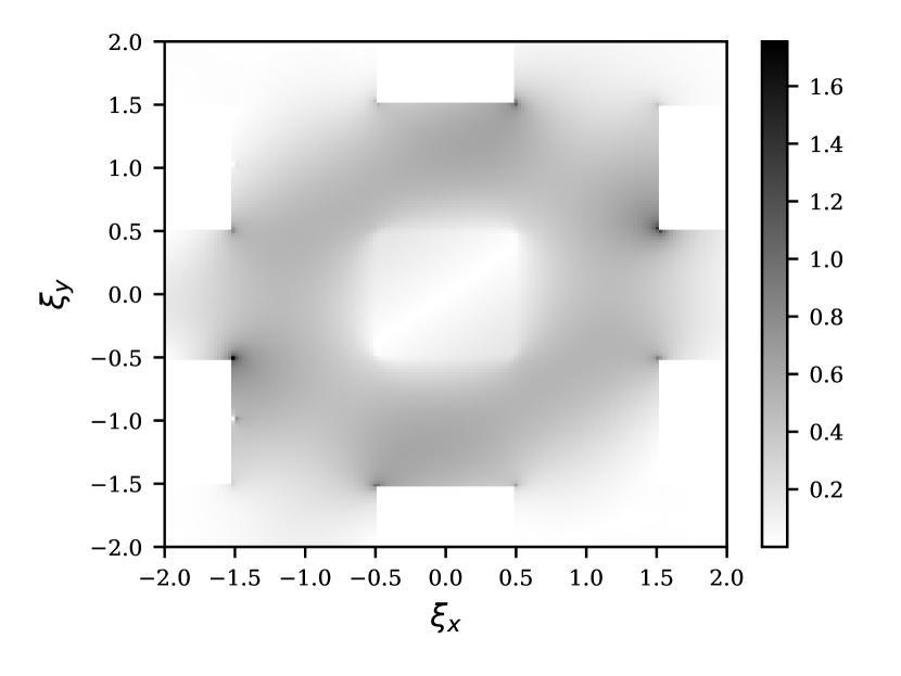
(b) $|\nabla_{\xi}\widehat{w}_{2}(\xi)|$, clearly showing the divergence on corners and discontinuity on edges.

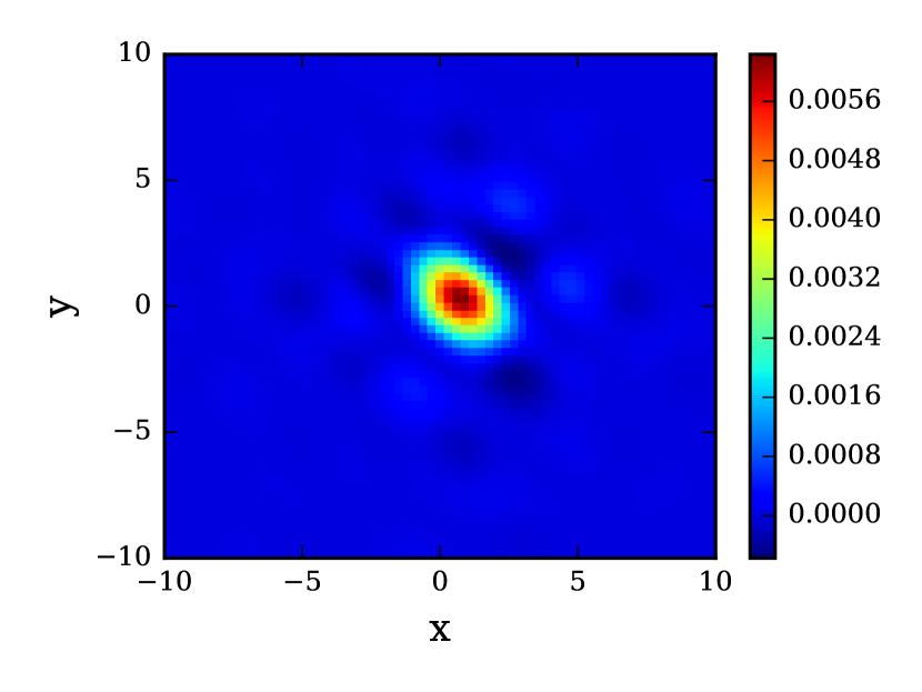
(c) $w_{2}(\mathbf{r})$.

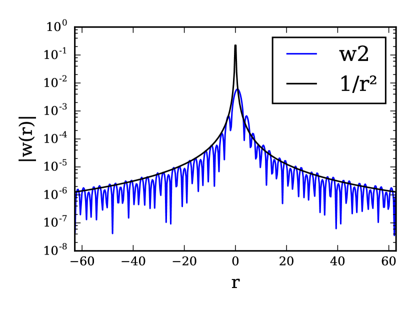
(d) Slice of $w_{2}$ at $y=0$, showing the $1/r^{2}$ decay.

Fig. 10: Second of four optimized Wannier functions for the free electron gas in 2D with one frozen band, on a $40\times 40$ $k$-point grid. The other three Wannier functions are similar to $w_{2}$.

5.3 Discussion

These results show that the maximally-localized Wannier functions only decay algebraically in general. Although numerical results are harder to obtain for real materials, we expect our analysis to carry through: an eigenvalue crossing at a particular $\mathbf{k}$ point acts as a constraint on the gauge, which must at that point be able to span the crossing eigenspace for the gauge to be continuous. Minimizing the second moments of the Wannier functions yields a gauge with a square-integrable but discontinuous first derivative at the crossing points, resulting in a weak localization.

Our findings are to be contrasted with the recent theoretical result of [7], which proves under generic hypotheses that there exists almost-exponentially localized Wannier functions. This simply means that, unlike in the case of insulators, for entangled band structures minimizing the second moments is not an asymptotically optimal strategy.

To get a faster asymptotic decay, one could minimize higher moments. This corresponds to minimizing integrals of higher derivatives, which have to be approximated by more complex stencils, and require the computation of additional overlaps between the $u_{n\mathbf{k}}$ than simply the nearest neighbors. This becomes numerically expensive and complex to implement. Another possibility is to perform local “smoothing surgeries” similar to the one we demonstrated in one dimension. This is likely to be useful only for very fine $\mathbf{k}$-point grids however.

6 Conclusion and discussion

We have developed a variational formulation that, paired with a specific initialization strategy, is able to robustly construct Wannier functions for systems with entangled band structure. Importantly, the definition of Wannier functions must be generalized, allowing them to lie in a subspace that contains, but is larger than, the spectral subspace of interest. While this condition adds extra constraints to our optimization problem, and they can be phrased in many theoretically equivalent ways, we find one that is particularly convenient. This results in a formulation that matches that of partly occupied Wannier functions [37], and allows us to view the widely used disentanglement procedure as an alternating minimization algorithm—albeit one that only takes a single alternation step. As the underlying problem is non-convex, our choice of initialization strategy via the SCDM methodology is key. As demonstrated with several real materials, our method is robust and effective at finding localized functions and enabling good quality band interpolation. Our variational formulation is versatile, and can be modified relatively easily to accommodate additional constraints, such as symmetry constraints, for certain type of real materials. It would also be interesting to study the behavior of localization properties of generalized Wannier functions for systems with non-trivial topological characters.

We also study the free electron gas, providing interesting insights into the further theoretical study of the localization properties of generalized Wannier functions. We find that the minimization of the second moments of the Wannier functions only imposes a relatively weak algebraic decay. Our analysis suggests that, for real 3D materials, the disentangled Wannier functions decay asymptotically slowly as well. Further localization is possible, but the method we present here is likely to only be useful for very fine $\mathbf{k}$-point grids. The computation of Wannier functions that are localized in both the pre-asymptotic and asymptotic regime remains an interesting open question.

Appendix A Gradient of the objective function

If $F$ is a function from a complex Hilbert space to $\mathbb{R}$, we recall that its gradient (sometimes written $\partial F/\partial z^{*}$) is defined as the (unique) vector $g$ such that

$$F(z+h)=F(z)+\mathrm{Re}~{}\left\langle g,h\right\rangle+O(h^{2}).$$

All the derivatives and gradient below are in this sense. Note that this is different from the notion of derivative of a $\mathbb{C}\to\mathbb{C}$ function, which is not relevant here (non-trivial complex-to-real functions are not complex differentiable). The advantage of this definition is that it allows a straightforward translation of first-order (but not second-order) optimization algorithms in complex variables.

We use the numerical setup of [27]. Recall that the $\mathbf{k}$-point grid is discretized, with a total of $N_{\mathbf{k}}$ points, and on each $\mathbf{k}$ in that grid, we are given a set of $N_{g}\times N_{o}$ matrices $u_{\mathbf{k}}$ representing the $N_{o}$ orbitals in the outer window discretized on a space of dimension $N_{g}$. The vectors $\{\mathbf{b}\}$ are displacements from one $\mathbf{k}$-point to a set of neighbors, and $w_{\mathbf{b}}$ are weights chosen to satisfy

$$\sum_{\mathbf{b}}w_{\mathbf{b}}\mathbf{b}\mathbf{b}^{T}=I_{3},$$

so that the gradient of a function $f(\mathbf{k})$ can be approximated by

$$\nabla f(\mathbf{k})\approx\sum_{\mathbf{b}}w_{\mathbf{b}}(f(\mathbf{k}+\mathbf{b})-f(\mathbf{k}))\mathbf{b}$$

We look for a set of $N_{o}\times N_{w}$ matrices $\{U_{\mathbf{k}}\}$ with orthogonal columns, which define Wannier functions by (13). Let

$$M_{\mathbf{k},\mathbf{b},m,n}=\langle u_{m,\mathbf{k}},u_{n,\mathbf{k}+\mathbf{b}}\rangle$$

be the $N_{o}\times N_{o}$ overlap matrix between the bands, which is an input of the algorithm. Then the $N_{w}\times N_{w}$ overlap matrix between the Wannier functions defined by $U(\mathbf{k})$ is

$$N_{\mathbf{k},\mathbf{b}}=U_{\mathbf{k}}^{*}M_{\mathbf{k},\mathbf{b}}U_{\mathbf{k}+\mathbf{b}}.$$

The Marzari-Vanderbilt spread functional is given by

$$\Omega =\sum_{n}\left\langle|\mathbf{r}|^{2}\right\rangle_{n}-|\left\langle\mathbf{r}\right\rangle_{n}|^{2},\text{ where}$$

$$\left\langle\mathbf{r}^{2}\right\rangle_{n} =\frac{1}{N_{\mathbf{k}}}\sum_{\mathbf{k},\mathbf{b}}w_{\mathbf{b}}\left(1-|N_{\mathbf{k}\mathbf{b}nn}|^{2}+(\mathrm{Im}~{}\ln N_{\mathbf{k}\mathbf{b}nn})^{2}\right)$$

$$\left\langle\mathbf{r}\right\rangle_{n} =-\frac{1}{N_{\mathbf{k}}}\sum_{\mathbf{k},\mathbf{b}}w_{\mathbf{b}}\mathrm{Im}~{}\ln N_{\mathbf{k}\mathbf{b}nn}\mathbf{b}$$

(equations (11), (31) and (32) of [27]).

We need to compute $\Omega(U+\Delta U)$ to first order in $\Delta U$, from which we will identify $\nabla\Omega$ by $\Omega(U+\Delta U)-\Omega(U)=\mathrm{Re}~{}\sum_{\mathbf{k}}\mathrm{Tr}((\nabla\Omega)_{\mathbf{k}}^{*}(\Delta U)_{\mathbf{k}})+O(\Delta U^{2})$.

We begin with $\sum_{n}\langle|\mathbf{r}|^{2}\rangle_{n}$ and consider the following quantity:

$$I=\sum_{\mathbf{k}\mathbf{b}n}f(N_{\mathbf{k}\mathbf{b}nn})$$

where $f:\mathbb{C}\to\mathbb{R}$. Then, using the fact that the set of vectors $\mathbf{b}$ is symmetric (contains $\mathbf{b}$ as well as $-\mathbf{b}$), and that $w_{-\mathbf{b}}=w_{\mathbf{b}}$,

$$\Delta I =\mathrm{Re}~{}\sum_{\mathbf{k}\mathbf{b}n}f^{\prime\prime}(N_{\mathbf{k}\mathbf{b}nn})^{*}\Delta N_{\mathbf{k}\mathbf{b}nn}$$

$$=\mathrm{Re}~{}\sum_{\mathbf{k}\mathbf{b}n}w_{\mathbf{b}}f^{\prime}(N_{\mathbf{k}\mathbf{b}nn})^{*}(\Delta A_{\mathbf{k}}^{*}M_{\mathbf{k}\mathbf{b}}A_{\mathbf{k}+\mathbf{b}})_{nn}+f^{\prime}(N_{\mathbf{k}\mathbf{b}nn})(\Delta A_{\mathbf{k}+\mathbf{b}}^{*}M_{\mathbf{k}\mathbf{b}}^{*}A_{\mathbf{k}})_{nn}$$

$$=\mathrm{Re}~{}\sum_{\mathbf{k}\mathbf{b}n}w_{\mathbf{b}}f^{\prime}(N_{\mathbf{k}\mathbf{b}nn})^{*}(\Delta A_{\mathbf{k}}^{*}M_{\mathbf{k}\mathbf{b}}A_{\mathbf{k}+\mathbf{b}})_{nn}+f^{\prime}(N_{\mathbf{k}-\mathbf{b},\mathbf{b},nn})(\Delta A_{\mathbf{k}}^{*}M_{\mathbf{k}-\mathbf{b},\mathbf{b}}^{*}A_{\mathbf{k}-\mathbf{b}})_{nn}$$

$$=\mathrm{Re}~{}\sum_{\mathbf{k}\mathbf{b}n}w_{\mathbf{b}}f^{\prime}(N_{\mathbf{k}\mathbf{b}nn})^{*}(\Delta A_{\mathbf{k}}^{*}M_{\mathbf{k}\mathbf{b}}A_{\mathbf{k}+\mathbf{b}})_{nn}+f^{\prime}(N_{\mathbf{k},-\mathbf{b},nn}^{*})(\Delta A_{\mathbf{k}}^{*}M_{\mathbf{k},-\mathbf{b}}^{*}A_{\mathbf{k}-\mathbf{b}})_{nn}$$

$$=\mathrm{Re}~{}\sum_{\mathbf{k}\mathbf{b}n}w_{\mathbf{b}}(f^{\prime}(N_{\mathbf{k}\mathbf{b}nn})^{*}+f^{\prime}(N_{\mathbf{k}\mathbf{b}nn}^{*}))(\Delta A_{\mathbf{k}}^{*}M_{\mathbf{k}\mathbf{b}}A_{\mathbf{k}+\mathbf{b}})_{nn}$$

and the gradient is therefore

$$(\nabla I)_{\mathbf{k}mn} =\sum_{\mathbf{b}}w_{\mathbf{b}}(f^{\prime}(N_{\mathbf{k}\mathbf{b}nn})^{*}+f^{\prime}(N_{\mathbf{k}\mathbf{b}nn}^{*}))(M_{\mathbf{k}\mathbf{b}}A_{\mathbf{k}+\mathbf{b}})_{mn}$$

It can be checked using similar arguments that, when

$$I=\sum_{\mathbf{k}\mathbf{b}n}\mathbf{b}g(N_{\mathbf{k}\mathbf{b}nn}),$$

then

$$(\nabla I)_{\mathbf{k}mn} =-\sum_{\mathbf{b}}w_{\mathbf{b}}(g^{\prime}(N_{\mathbf{k}\mathbf{b}nn})^{*}+g^{\prime}(N_{\mathbf{k}\mathbf{b}nn}^{*}))(M_{\mathbf{k}\mathbf{b}}A_{\mathbf{k}+\mathbf{b}})_{mn}\mathbf{b}$$

Applying these formulas with

$$f(z) =1-|z|^{2}+(\mathrm{Im}~{}\ln z)^{2},\quad f^{\prime}(z)=-2z+2\frac{i\mathrm{Im}~{}\ln z}{z^{*}}$$

$$g(z) =-\mathrm{Im}~{}\ln z,\quad g^{\prime}(z)=-\frac{i}{z^{*}}$$

we get

$$(\nabla\Omega)_{\mathbf{k}mn} =\frac{4}{N_{\mathbf{k}}}\sum_{\mathbf{b}}\left(-N_{\mathbf{k}\mathbf{b}nn}^{*}-i\frac{\mathrm{Im}~{}\ln N_{\mathbf{k}\mathbf{b}nn}+\left\langle r\right\rangle_{n}\cdot\mathbf{b}}{N_{\mathbf{k}\mathbf{b}nn}}\right)(M_{\mathbf{k}\mathbf{b}}A_{\mathbf{k}+\mathbf{b}})_{mn}$$

Note that this is the unconstrained gradient of $\Omega$ with respect to $U$. Using the chain rule one with $U(\mathbf{k})=\begin{bmatrix}I_{N_{f}}&0\\ 0&Y\end{bmatrix}X$ one can easily derive the gradient of $\Omega$ with respect to $(X,Y)$. Then we simply have to minimize with respect to $(X,Y)$ subject to the orthogonality constraints for $X$ and $Y$ using standard methods [13, 1].

References

- [1] P-A. Absil, R. Mahony, and R. Sepulchre, Optimization algorithms on matrix manifolds, Princeton University Press, 2009.
- [2] J. Bezanson, A. Edelman, S. Karpinski, and V.B. S., Julia: A fresh approach to numerical computing, SIAM Review, 59 (2017), pp. 65–98.
- [3] E. I. Blount, Formalisms of band theory, Solid State Phys., 13 (1962), pp. 305–373.
- [4] D. R. Bowler and T. Miyazaki, O(N) methods in electronic structure calculations, Rep. Prog. Phys., 75 (2012), p. 036503.
- [5] C. Brouder, G. Panati, M. Calandra, C. Mourougane, and N. Marzari, Exponential localization of Wannier functions in insulators, Phys. Rev. Lett., 98 (2007), p. 046402.
- [6] E. Cancès, A. Levitt, G. Panati, and G. Stoltz, Robust determination of maximally-localized Wannier functions, Phys. Rev. B, 95 (2017), p. 075114.
- [7] H. Cornean, D. Gontier, A. Levitt, and D. Monaco, Localised wannier functions in metallic systems. in preparation, 2017.
- [8] A. Damle and L. Lin, Disentanglement via entanglement: A unified method for wannier localization, arXiv:1703.06958, (2017).
- [9] A. Damle, L. Lin, and L. Ying, Compressed representation of Kohn–Sham orbitals via selected columns of the density matrix, J. Chem. Theory Comput., 11 (2015), pp. 1463–1469.
- [10] Anil Damle, Lin Lin, and Lexing Ying, Scdm-k: Localized orbitals for solids via selected columns of the density matrix, J. Comput. Phys., 334 (2017), pp. 1 – 15.
- [11] M. Dauge, Elliptic boundary value problems on corner domains: smoothness and asymptotics of solutions, vol. 1341, Springer, 2006.
- [12] W. E, T. Li, and J. Lu, Localized bases of eigensubspaces and operator compression, Proc. Natl. Acad. Sci., 107 (2010), pp. 1273–1278.
- [13] A. Edelman, T.A. Arias, and S.T. Smith, The geometry of algorithms with orthogonality constraints, SIAM journal on Matrix Analysis and Applications, 20 (1998), pp. 303–353.
- [14] J. M. Foster and S. F. Boys, Canonical configurational interaction procedure, Rev. Mod. Phys., 32 (1960), p. 300.
- [15] Paolo Giannozzi, Stefano Baroni, Nicola Bonini, Matteo Calandra, Roberto Car, Carlo Cavazzoni, Davide Ceresoli, Guido L Chiarotti, Matteo Cococcioni, Ismaila Dabo, Andrea Dal Corso, Stefano de Gironcoli, Stefano Fabris, Guido Fratesi, Ralph Gebauer, Uwe Gerstmann, Christos Gougoussis, Anton Kokalj, Michele Lazzeri, Layla Martin-Samos, Nicola Marzari, Francesco Mauri, Riccardo Mazzarello, Stefano Paolini, Alfredo Pasquarello, Lorenzo Paulatto, Carlo Sbraccia, Sandro Scandolo, Gabriele Sclauzero, Ari P Seitsonen, Alexander Smogunov, Paolo Umari, and Renata M Wentzcovitch, QUANTUM ESPRESSO: a modular and open-source software project for quantum simulations of materials, J. Phys.: Condens. Matter, 21 (2009), pp. 395502–395520.
- [16] S. Goedecker, Linear scaling electronic structure methods, Rev. Mod. Phys., 71 (1999), pp. 1085–1123.
- [17] F. Gygi, Compact representations of Kohn–Sham invariant subspaces, Phys. Rev. Lett., 102 (2009), p. 166406.
- [18] William W Hager and Hongchao Zhang, A new conjugate gradient method with guaranteed descent and an efficient line search, SIAM Journal on optimization, 16 (2005), pp. 170–192.
- [19] P. Hohenberg and W. Kohn, Inhomogeneous electron gas, Phys. Rev., 136 (1964), pp. B864–B871.
- [20] E. Koch and S. Goedecker, Locality properties and Wannier functions for interacting systems, Solid State Commun., 119 (2001), p. 105.
- [21] W. Kohn, Analytic properties of Bloch waves and Wannier functions, Phys. Rev., 115 (1959), p. 809.
- [22] , Density functional and density matrix method scaling linearly with the number of atoms, Phys. Rev. Lett., 76 (1996), pp. 3168–3171.
- [23] W. Kohn and L. Sham, Self-consistent equations including exchange and correlation effects, Phys. Rev., 140 (1965), pp. A1133–A1138.
- [24] P. Kuchment, An overview of periodic elliptic operators, Bulletin of the American Mathematical Society, 53 (2016), pp. 343–414.
- [25] P.-O. Löwdin, On the non-orthogonality problem connected with the use of atomic wave functions in the theory of molecules and crystals, J. Chem. Phys., 18 (1950), pp. 365–375.
- [26] N. Marzari, A. A. Mostofi, J. R. Yates, I. Souza, and D. Vanderbilt, Maximally localized Wannier functions: Theory and applications, Rev. Mod. Phys., 84 (2012), pp. 1419–1475.
- [27] N. Marzari and D. Vanderbilt, Maximally localized generalized Wannier functions for composite energy bands, Phys. Rev. B, 56 (1997), p. 12847.
- [28] A.A. Mostofi, J.R. Yates, Y.S. Lee, I. Souza, D. Vanderbilt, and N. Marzari, Wannier90: a tool for obtaining maximally-localised Wannier functions, Comput. Phys. Commun., 178 (2008), p. 685.
- [29] A. Mostofi, J.R. Yates, G. Pizzi, Y. Lee, I. Souza, D. Vanderbilt, and N. Marzari, An updated version of wannier90: A tool for obtaining maximally-localised Wannier functions, Computer Physics Communications, 185 (2014), pp. 2309–2310.
- [30] J. I. Mustafa, S. Coh, M. L. Cohen, and S. G. Louie, Automated construction of maximally localized Wannier functions: Optimized projection functions method, Phys. Rev. B, 92 (2015), p. 165134.
- [31] G. Nenciu, Dynamics of band electrons in electric and magnetic fields: rigorous justification of the effective hamiltonians, Rev. Mod. Phys., 63 (1991), pp. 91–127.
- [32] J. Nocedal and S.J. Wright, Numerical optimization, Springer, 2006.
- [33] V. Ozoliņš, R. Lai, R. Caflisch, and S. Osher, Compressed modes for variational problems in mathematics and physics, Proc. Natl. Acad. Sci., 110 (2013), pp. 18368–18373.
- [34] G. Panati, Triviality of Bloch and Bloch–Dirac bundles, in Annales Henri Poincaré, vol. 8, Springer, 2007, pp. 995–1011.
- [35] G. Panati and A. Pisante, Bloch bundles, Marzari-Vanderbilt functional and maximally localized Wannier functions, Commun. Math. Phys., 322 (2013), pp. 835–875.
- [36] I. Souza, N. Marzari, and D. Vanderbilt, Maximally localized wannier functions for entangled energy bands, Phys. Rev. B, 65 (2001), p. 035109.
- [37] K. S. Thygesen, L. B. Hansen, and K. W. Jacobsen, Partly occupied wannier functions, Phys. Rev. Lett., 94 (2005), p. 026405.
- [38] J. von Neumann and E.P. Wigner, Über merkwürdige diskrete eigenwerte, in The Collected Works of Eugene Paul Wigner, Springer, 1993, pp. 291–293.
- [39] G. H. Wannier, The structure of electronic excitation levels in insulating crystals, Phys. Rev., 52 (1937), p. 191.
- [40] J. R. Yates, X. Wang, D. Vanderbilt, and I. Souza, Spectral and Fermi surface properties from Wannier interpolation, Phys. Rev. B, 75 (2007), p. 195121.