Strong dipole magnetic fields in fast rotating fully convective stars

Abstract

M dwarfs are the most numerous stars in our Galaxy with masses between approximately $0.5$ and $0.1$ solar mass. Many of them show surface activity qualitatively similar to our Sun and generate flares, high X-ray fluxes, and large-scale magnetic fields[1, 2, 3, 4]. Such activity is driven by a dynamo powered by the convective motions in their interiors[5, 2, 6, 7, 8]. Understanding properties of stellar magnetic fields in these stars finds a broad application in astrophysics, including, e.g., theory of stellar dynamos and environment conditions around planets that may be orbiting these stars. Most stars with convective envelopes follow a rotation-activity relationship where various activity indicators saturate in stars with rotation periods shorter than a few days[2, 6, 8]. The activity gradually declines with rotation rate in stars rotating more slowly. It is thought that due to a tight empirical correlation between X-ray and magnetic flux[9], the stellar magnetic fields will also saturate, to values around $\sim 4$ kG[10]. Here we report the detection of magnetic fields above the presumed saturation limit in four fully convective M-dwarfs. By combining results from spectroscopic and polarimetric studies we explain our findings in terms of bistable dynamo models[11, 12]: stars with the strongest magnetic fields are those in a dipole dynamo state, while stars in a multipole state cannot generate fields stronger than about four kilogauss. Our study provides observational evidence that dynamo in fully convective M dwarfs generates magnetic fields that can differ not only in the geometry of their large scale component, but also in the total magnetic energy.

Institute for Astrophysics, Georg-August University, Friedrich-Hund-Platz 1, D-37077 Göttingen, Germany

Canada-France-Hawaii Telescope (CFHT) Corporation, 65-1238 Mamalahoa Highway, Kamuela, Hawaii 96743, USA

Institut de recherche sur les exoplanétes (iREx), Département de Physique, Université de Montréal, Montréal, QC H3C 3J7

Harvard-Smithsonian Center for Astrophysics, 60 Garden Street, Cambridge, MA 02138, USA

LUPM, Universite de Montpellier, CNRS, place E. Bataillon, F-34095 Montpellier, France

Department Physics and Astronomy, Uppsala University, Box 516, 751 20, Uppsala, Sweden

notmainnot segment=

Our understanding of origin and evolution of the magnetic fields in M dwarfs is based on the models of the rotationally driven convective dynamos. Modern observations provide two important constraints for these models.

First, from the analysis of circular polarization in spectral lines we infer that large-scale magnetic fields tend to have simple axisymmetric geometry with dominant poloidal component in stars that are fully convective. In contrast, M dwarfs that are hotter and therefore only partly convective tend to have more complex fields with strong toroidal components[13]. However, there is a number of exceptions when a rapidly-rotating fully convective star generates a large-scale magnetic field with a complex multipole geometry. This dichotomy of magnetic properties in stars that have similar stellar parameters may be explained in terms of dynamo bistability: stars can relax to either dipole or multipole states depending on the geometry and the amplitude of an initial seed magnetic field[11, 12]. Note, however, that dynamo bistability was observed only in models of stars with masses $M\leqslant 0.2M_{\odot}$.

The second observational constraint is the rotation–activity relation[2, 14, 8, 15]. A remarkable feature of this relation is the existence of two branches, a saturated and a non-saturated branch. In the non-saturated branch, the amount of non-thermal (e.g., X-ray) emission generated by the star grows with rotation rate. On the saturated branch (corresponding rotation periods shorter than $\sim 4$ days) the level of activity shows only little dependence on rotation.

In observations of solar active regions and some young stars, absolute X-ray luminosity was found to be proportional to magnetic flux[9] ($4\pi R^{2}\langle B\rangle$, i.e., surface area of the star times magnetic flux density). This correlation suggests that, as long as X-ray luminosity saturates in fast rotating stars, a similar saturation of the magnetic flux (and/or magnetic flux density) may also take place. A growing database of stellar magnetic field measurements showed that the strength of the maximum possible surface magnetic field reaches values around $3-4$ kG in the coolest M dwarf stars[16, 17, 18, 10, 19]. Mean fields stronger than this have not been detected in any low-mass star, which was viewed as an evidence for the magnetic field saturation[10]. It occurs for stars with rotational periods shorter than a few days implying that the generation of magnetic flux itself does not grow beyond a level proportional to the bolometric luminosity, as supported by theoretical studies[20]. Strong kilogauss level magnetic fields are equally found in stars with dipole and multipole states suggesting that these stars may share a common mechanism of saturation.

Measurements of the magnetic fields in M dwarfs usually utilize either unpolarized light (Stokes-$\rm I$), or circularly polarized light (Stokes-$\rm V$). The important difference between the two is that Stokes-$\rm V$ carries information about polarity and geometry of the magnetic field which is organized at large spatial scales on the stellar surface. However, Stokes-$\rm V$ can not see small scale magnetic fields because these fields have different polarities and thus their contribution is canceled out when the star is observed from a large distance as a point source. To the contrary, both large and small scale fields contribute to the unpolarized Stokes-$\rm I$ light. Thus, using Stokes-$\rm I$ one can measure the strength of the total magnetic field[21]. However, all previous studies made use primarily of either Stokes-$\rm I$ or Stokes-$\rm V$ radiation without detailed analysis of the link between the two. For instance, it was known[22] that Stokes-$\rm V$ measurements can miss up to $90$% of the total magnetic flux density of the star, while for many stars with published Stokes-$\rm V$ magnetic maps only coarse measurements of the magnetic field strength from Stokes-$\rm I$ were available.

The analysis of the magnetic fields has significantly improved over the last decade thanks to development of new methods and techniques, making it possible to look at magnetic properties of stars in more detail. In our research we used data collected over several years with the twin spectropolarimeters ESPaDOnS and NARVAL mounted at the $3.6$ m Canada-France-Hawaii Telescope (CFHT) and the $2$ m Telescope Bernard Lyot (TBL) at the Pic du Midi (France), respectively[23]. Both instruments cover a spectral range between $367-1050$ nm and have spectral resolution $R\approx 65,000$ (in polarimetric mode). We chose a sample of M dwarfs with known rotational periods and available magnetic maps derived from inversion of Stokes-$\rm V$ spectra[13, 24]. The ultimate aim of our work is to measure magnetic flux density from independent spectroscopic diagnostics by utilizing up-to-date radiative transfer modelling. Contrary to previous studies we analyze Stokes-$\rm I$ spectra because we want to capture the total magnetic flux which provides essential constraints for the underlying dynamo mechanism.

Our analysis resulted in the detection of very strong magnetic fields in four M dwarf stars. We report the strongest average magnetic field $\langle B\rangle\approx 7.0$ kG in the star WX UMa (Gl 412 B), a field of $\langle B\rangle\approx 6.0$ kG in stars Wolf 47 (Gl 51) and UV Cet (Gl 65 B), and a field about $5.0$ kG in V374 Peg, respectively. Note that WX UMa is the only cool active star known to date where the Zeeman splitting in single atomic lines is clearly observed at optical wavelengths (Zeeman splitting at long near-infrared wavelengths is easier to see and therefore it has already been detected in some objects[16, 25]). Figure 1 demonstrates example fits to magnetically sensitive spectral lines in these and in three other magnetic M dwarfs that we have chosen for comparison. For WX UMa we measure a minimum magnetic field of about $6$ kG from Zeeman splitting in Rb I $\lambda 794.76$ nm and Ti I $\lambda 837.7$ nm lines, and larger values when applying radiative transfer model to fit full line profiles.

WX UMa is an unusual object: it is a rapid rotator (rotation period $P=0.74$d) but it has relatively low inclination angle $i=40$^∘ of its rotation axis with respect to the observer. This results in relatively small projected rotational velocity $\upsilon\sin i\approx 6$ km s^-1 and corresponding rotation broadening of spectral lines become weaker than the magnetic one. This is why we could detect the Zeeman splitting in atomic lines in this star. For instance, in Wolf 47 we also measure a very strong field, but high $\upsilon\sin i\approx 11$ km s^-1 makes it impossible to observe corresponding Zeeman splitting in this star (see Fig. 1). In our final measurements of magnetic fields we use numerous lines of FeH molecule at $\lambda\lambda 990-995$ nm (Wing-Ford $F^{4}\,\Delta-X^{4}\,\Delta$ transitions) and near-infrared Ti lines located between $960-980$ nm. The details of our analysis are given in section Methods. Thus, we report for the first time a definite detection of the magnetic fields in M dwarfs well beyond its recent maximum value of about four kilogauss. Our Fig. 2 demonstrates that new detection make a clear difference because they substantially extend the range of measured to date magnetic fields in stars with saturated activity level.

Our discovery allows us to draw several important conclusions. First we note that, according to published magnetic field maps, WX UMa and Wolf 47 belong to the dipole branch and show concentration of strong magnetic fields around rotation poles (so-called magnetic polar caps)[13]. In contrast to this, none of the multipole stars with similar parameters and rotation rates exhibits a field stronger than $\langle B\rangle\sim 4$ kG. Thus our analysis implies that stars with dipole states may generate stronger fields compared to stars with multipole states at the same rotation rate. This conclusion is in agreement with the predictions of bistable dynamo models[11, 12].

Next, we emphasize that the magnetic field we derive in stars with a dipole dominated geometry does not necessarily reflect the surface-averaged magnetic flux density. Indeed, because of geometric projection, we observe fields stronger than the surface average field in stars oriented to us with their magnetic poles, and weaker fields is stars that rotate equally fast but seen equator-on. From the magnetic maps corresponding to dynamo models[26] we estimate that WX UMa with its $7.3$ kG magnetic field and inclination of $i=40$^∘ would show “only” $6.4$ kG should it had the inclination $i=60$^∘, which matches well enough the field that we measure in, e.g., Wolf 47 which has $i=60$^∘[13]. The magnetic flux density averaged over whole stellar surface for WX UMa amounts now to $6.8$ kG (against measured $7.3$ kG), which is still significantly higher than the maximum field strength in stars with multipole regime. (See our Supplementary Fig. 1 for the visualization of the geometrical effect). Note that this geometrical effect should be absent in stars with multipole fields because these fields are randomly distributed over stellar surface without any preferred axis.

By analyzing the dependence between measured magnetic field and rotation period we observe that the magnetic flux density in stars with dipole-dominated geometry still grows with rotation rate. In Fig. 3 we plot our magnetic field measurements for all M dwarfs with known magnetic geometries[13, 24]. We find the same trend of increasing magnetic field strength as rotation periods decrease to about four days (so-called unsaturated regime), as was found in previous studies[10]. However, we now show that magnetic fields in M dwarfs with multipole dynamo state saturate below periods of about four days with the saturated magnetic flux density $\langle B\rangle\sim 4$ kG (corresponding Rossby number $Ro=P/\tau_{\rm c}<0.1$, where $P$ is the stellar rotation period and $\tau_{\rm c}$ is the convective turnover time, see Supplementary Fig. 2), while some stars with dipole state exhibit surface fields unambiguously above $4$ kG and demonstrate no obvious saturation effect. However, from our limited data set it remains unclear whether these stars saturate at faster rotation or if the saturation value for the magnetic field is only stronger, in comparison to stars with multipole state. Nevertheless, from this plot we can see that dynamo processes may behave differently with rotation rate in dipole and multipole branches. It is thus important to address this question with future observations in more detail.

An alternative explanation of the dichotomy in magnetic field geometries is to assume that M dwarfs can have magnetic cycles during which magnetic field can change its geometry and strength over cycle period. This would explain the difference in magnetic fields between individual objects. Note that the signs of activity cycles were found in some M dwarfs stars based on photometric/spectroscopic observations[27], including a recent detection of a clear $7$ year photometric cycle in fully convective and slowly rotating ($P\approx 83$d) M dwarf Proxima Centauri[28]. By computing a model for this star it was shown that dynamo in fully convective M dwarfs can indeed generate magnetic cycles with repeated reversals of the magnetic polarities at different latitudes with time, provided that these stars rotate slow enough to develop differential rotation in their convection zones[29]. On the other hand, same models showed that as rotation increases, the generated magnetic fields finally become strong enough to quench the differential rotation and thus no magnetic cycles are expected: once reached, a star never changes its dynamo state. This theoretical prediction is supported by ZDI observations of fast rotating ($Ro<0.1$) M dwarfs, though magnetic cycles could be as long as decades in these stars[30]. Thus, to test which of the two scenarios (i.e., bistable dynamo vs. cyclic dynamo) is responsible for the observed magnetic properties of M dwarfs a long-term spectropolarimetric monitoring is required.

This project was carried out in the framework of the DFG funded CRC 963 – Astrophysical Flow Instabilities and Turbulence (projects A16 and A17). We acknowledge support from the DAAD strategic partnership project U4-Network to D.S. and funding through a Heisenberg Professorship RE 1664/9-2 to A.R. R.K.Y is supported by NASA Chandra grant GO4-15011X. O.K. acknowledges funding from the Swedish Research Council and the Swedish National Space Board. We also acknowledge the use of electronic databases (VALD, SIMBAD, NASA’s ADS). This research is based on observations collected at the Canada-France-Hawaii Telescope (Hawaii) and Telescope Bernard Lyot (France).

D.S. contributed general scientific ideas and conclusions, carried out the processing, modelling, and analysis of observed data. A.R. contributed general scientific ideas and conclusions. A.E. carried out modelling and analysis of observed data. L.M. carried out telluric correction on selected targets. R.Y. provided theoretical dynamo models and magnetic maps. J.M. provided and analyzed additional Stokes-V data on some ESPaDOnS targets. O.K. contributed to development of atomic line analysis methodology. All authors contributed to the text of the paper and discussed the results.

Reprints and permissions information is available at www.nature.com/reprints. The authors declare no competing financial interests. Readers are welcome to comment on the online version of the paper. Correspondence and requests for materials should be addressed to D.S. (denis@astro.physik.uni-goettingen.de).

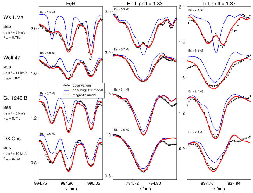
Figure 1: Magnetic field diagnostics in selected M dwarfs. We show example fits to magnetically sensitive spectral lines of FeH molecule (left column), Rb I $\lambda 794.76$ nm line (middle column), and Ti I $\lambda 837.7$ nm line (right column) in WX UMa and three other magnetic M dwarfs. Black dots – observed spectra; blue dashed line – predicted zero field model; red full line – predicted best fit magnetic model. The text on the left side lists for each stars its name, spectral class, projected rotational velocity $\upsilon\sin i$, rotational period, and surface average magnetic field. Rotation periods are taken from works on magnetic mapping[13]. The magnetic field was calculated from distributions of filling factors $\langle B\rangle=\sum_{i}B_{i}\cdot f_{i}$ (see Methods). Our measurements of $\langle B\rangle$ may vary with assumed stellar parameters (e.g., $T_{\rm eff}$, $\log(g)$) and we show here only one choosen solution. In case of WX UMa, a clear splitting is visible in atomic Rb I and Ti I lines, and the separation of Zeeman components corresponds to a minimum magnetic field of $\approx 6$ kG. Employing different $T_{\rm eff}$’s and spectral lines results in magnetic fields between $7.0$ kG and $7.5$ kG.

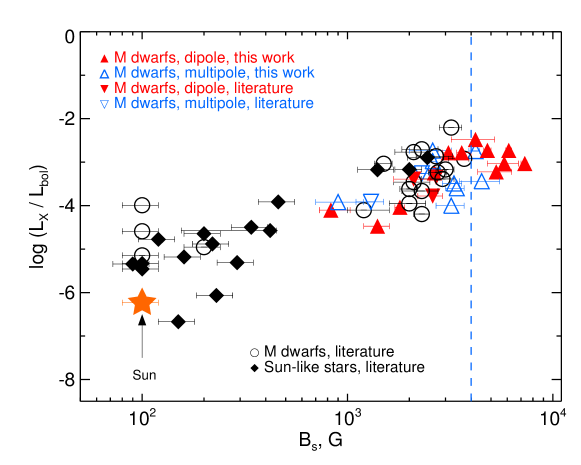
Figure 2: Magnetic field – activity relation. The plot illustrates activity level (in terms of X-ray luminosity, $L_{\rm x}$, normalized to bolometric luminosity $L_{\rm bol}$), as a function of magnetic field strength in cool stars. Red filled upward and downward triangles are M dwarfs with dipole dominant fields and measurements from this work and literature, respectively. Blue open upward and downward triangles are M dwarfs with multipole dominant fields and measurements from this work and literature, respectively. Black open circles are M dwarfs with unknown magnetic field configurations and measurements from the literature. Sun-like stars are shown with black filled diamonds: we plot these stars because they have interior structure similar to partly convective M dwarfs (e.g., both have outer convective zone and inner radiative core) and obey same rotation-activity relation[8]. The Sun is marked with the orange star symbol. Vertical blue dashed line marks the $4$ kG limit of the maximum magnetic field strength measured in early studies. It is seen that adding our new measurements substantially extends the range of possible mean magnetic fields in M dwarfs. The error bars on literature values are taken from original papers (see Supplementary Table 1), while errors on our measurements represent estimated uncertainty rather than formal fitting errors (see Fig. 3 and Supplementary Table 2 for more details and notes on individual objects).

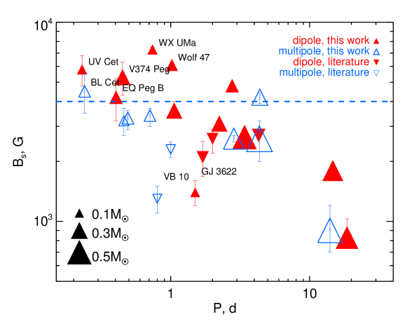
Figure 3: Rotation – magnetic field relation. We plot magnetic flux density fields in stars from our sample as a function of rotation period. Our new measurements in stars with dipole and multipole states are shown as red filled and blue open triangles, respectively. The red and blue upsidedown triangles represent stars with dipole and multipole states, respectively, and magnetic field measurements from the literature. The symbol size scales with stellar mass (see legend on the plot). The horizontal dashed line marks the $4$ kG threshold of saturated magnetic field assigned to stars with multipole dynamo regime. We demonstrate that stars with dipole state can still generate very strong magnetic fields even at very fast rotation while stars with multipole state saturate at rotation periods of about $4$d and fields about $\sim 4$ kG. Two stars, VB 10 and GJ 3622, have very weak magnetic fields as expected for their rotation periods. We explicitly mark them on the plot and note that it is important to cross check their rotation periods with future observations. Measurements from this work that we show on this figure are additionally listed in Supplementary Table 2. The error bars on literature values are taken from original papers (see Supplementary Table 1), while errors on our measurements represent estimated uncertainty rather than formal fitting errors (see Supplementary Table 2). It was calculated as a mean of the four independent measurements (two different effective temperatures and two different spectral regions containing FeH and Ti lines, respectively), with error bars being the amplitude of the scatter between these measurements. For stars with largest $\upsilon\sin i$’s, Bl Cet, UV Cet, V374 Peg and EQ Peg B, we compute final magnetic field from Ti lines only. We do this because FeH lines become strongly blended and tend to underestimate magnetic fields at cool temperatures due to degeneracy between magnetic field and Fe abundance (see section Methods for more details). Considering this and other uncertainties we put a conservative $1$ kG error bars on measured magnetic fields in these stars.

notmethodsnot segment=

Details on theoretical modelling.

Our strategy to measure Zeeman splitting is to compare observed spectra to synthetic spectra computed with a polarized radiative transfer code that is based on the custom routine taken from the model atmosphere code LLmodels[31] and extended by the complete treatment of polarized radiation in all four Stokes parameters[32]. The radiative transfer equation is solved with the DELO (Diagonal Element Lambda Operator) method[33, 34], which have proved their capabilities for accurate solution of the transfer equation.

In our equation of state we include $99$ atoms (from Hydrogen to Einsteinium) and $524$ molecules. This results in total of $930$ individual plasma components (i.e., atoms, molecules, and their ions). Most of atomic partition functions are those provided by R.L. Kurucz[35] (http://kurucz.harvard.edu). For molecules we utilize partition functions and equilibrium constants available from the literature[36, 37, 38, 39]. Molecular data can be used in wide temperature ranges from $1000$ K to $9000$ K, i.e., suitable for conditions found in atmospheres of M dwarf stars. The final system of linear equations is solved using LU factorization methods available from the LAPACK numerical library (http://www.netlib.org/lapack/). We tested solutions of our equation of state against those implemented in such codes as SYNTHE[35], SSynth[40], and Synth3[41], and found good agreement in resulting number densities of most abundant species.

We treat pressure broadening by including contributions from hydrogen and helium atoms only. Normally, a contribution from the molecular hydrogen H₂ is also expected. However, similar to previous studies[42], we find that inclusion of H₂ overestimates the widths of line profiles in benchmark inactive M dwarfs. This problem is most prominent in strong alkali lines. It increases with decreasing temperature and starts to affect noticeably other atomic and molecular lines, too.

Another source of line broadening is the velocity field caused by convective motions. However, as shown by 3D hydrodynamical simulations[43], the velocity fields in atmospheres of M dwarfs with temperatures $T_{\rm eff}<3500$ K are well below $1$ km s^-1. This only has a weak impact on line profiles, leaving the Zeeman effect and rotation to be the dominating broadening mechanisms. Therefore we assumed zero micro- and macroturbulent velocities in all calculations.

Representation of surface magnetic field.

Our analysis relies on unpolarized Stokes-$\rm I$ spectra, which means that we can measure the surface averaged magnetic flux density (or simply magnetic field strength) $\langle B\rangle$ from magnetically broadened line profiles but we derive no information about field geometry. Note that in case of complex magnetic fields localized in spots, spot groups, or active regions across the stellar surface, the mean magnetic field cannot be represented by a simple homogeneous magnetic field configuration. Instead, the best approximation is to assume that the total field is the weighted sum over different field components; $\langle B\rangle=\sum|\mathbf{B}|_{i}f_{i}$, where $f_{i}$ are corresponding filling factors that represent the fraction of the stellar surface covered by the magnetic field of the strength $|\mathrm{\mathbf{B}}|_{i}$. We use $11$ magnetic field components and corresponding filling factors are normalized so that $\sum f_{i}=1$. In case of stars with large $\upsilon\sin i$’s individual features in lines profiles caused by complex magnetic fields are usually not recoverable and we speed up computations by assuming two component model: non-magnetic and magnetic with a filling factor $f$ so that the total magnetic field strength is $\langle B\rangle=Bf$. In all computations we assumed that the magnetic field is dominated by its radial component[44].

Details on spectroscopic analysis.

In order to compute theoretical line profiles we used MARCS model atmospheres[45]. The effective temperatures of M dwarfs are not accurately known and different sources sometimes list noticeably different values. Therefore, we fit each star assuming two different temperatures. First is the one that follows from spectral types employing dedicated calibrations[46, 47]. The spectral types were taken from previous works on magnetic field measurements[4] and from the SIMBAD online service. In our second estimate of the $T_{\rm eff}$ we used lines of TiO $\gamma$-band at $705$ nm extracted from Vienna Atomic Line Database (VALD)[48, 49] with transition parameters calculated by B. Plez (private communication), version of 7 Mar 2012, with wavelengths corrected using polynomial fits to laboratory wavelengths[50, 51] (see Master thesis by T. Nordlander[52] http://urn.kb.se/resolve?urn=urn:nbn:se:uu:diva-174640). Our temperature estimates from TiO lines are in agreement (within error bars) with alternative independent estimates[53]. The other essential parameter – stellar gravity ($\log(g)$) – was calculated from the stellar radii and mass assuming $R\propto M^{0.9}$ relation which provides surface gravities close to those predicted by stellar evolution models[54, 55].

To derive magnetic fields we used two sets of spectral lines. First set includes lines of FeH molecule. In particular, we used lines of the Wing-Ford $F^{4}\,\Delta-X^{4}\,\Delta$ transitions between $\lambda\lambda 990.0-990.4$ nm and $\lambda\lambda 993.8-996.0$ nm regions, respectively. These lines are a perfect indicators of magnetic fields in cool stars because of their high magnetic sensitivity[56, 57]. The transition parameters of FeH molecule were taken from our previous investigations[44, 58, 59].

It is known that the Zeeman splitting in FeH lines could not be accurately predicted by available theoretical descriptions[60, 61] and alternative semi-empirical methods are used instead[62, 59]. Therefore, extending our analysis to atomic lines provides important independent constraints on the measured magnetic fields. Therefore, as the second set of magnetic field indicators, we choose to use Ti I lines in $\lambda\lambda 960-980$ nm region. These lines are originating from the same multiplet and thus their relative oscillator strengths are known with a high precision. Therefore it was enough to cross check the oscillator strengths of a few of these lines visible in the spectrum of the Sun[63] to make sure that we do not introduce any biases in our analysis. These Ti lines have very different magnetic sensitivity with Landé g-factors ranging from $0$ to $1.55$ and different Zeeman patterns which makes them very good diagnostics of the magnetic fields. In addition, we analyzed profiles of Ti I $\lambda 837.7$ nm and Rb I $\lambda 794.8$ nm lines that show a clear Zeeman splitting in WX UMa, but because of very strong blending by TiO molecule in this spectral region we could not use these two lines for the final magnetic field measurements in all stars. Instead, we use Rb I $\lambda 794.8$ nm and Ti I $\lambda 837.7$ nm only in Fig. 1 for illustrative purpose only, i.e., to highlight a very strong magnetic field in WX UMa. Transition parameters of all atomic lines were extracted from VALD.

When the $\upsilon\sin i$ of a star is large, our measurements rely on the effect of magnetic intensification of spectral lines[64] which predicts that the depth of a magnetic sensitive line broadened by rotation will be increased depending on its Zeeman pattern. Of course, this technique is sensitive to fields that are strong enough to produce observable changes in the equivalent widths of lines (see, e.g., Supplementary Fig. 9 for a clear example of magnetic intensification influencing profiles of spectral lines). The Ti I lines in $\lambda\lambda 960-980$ nm region are therefore superior diagnostic of strong fields in fast rotating stars and we successfully used their magnetic intensification in our analysis. The reason why these lines are normally completely ignored in spectroscopic studies is because they are heavily contaminated by telluric absorption from the Earth atmosphere. Considering the importance of these lines for our goals we made an effort of removing telluric absorption from all stellar spectra of all stars by applying the molecfit software package[65, 66].

We use the Levenberg-Marquardt minimization algorithm to find best fit values of filling factors for a given combination of atmospheric parameters[44]. We simultaneously treat rotational velocity $\upsilon\sin i$, atmospheric abundance of a given element, continuum scaling factor for each spectral region that we fit, and $11$ filling factors distributed between $0$ kG and $10$ kG as free parameters. (For stars with very strong field it was sometimes necessary to use wider range of magnetic filling factors, i.e., $11$ filling factors distributed between $0$ kG and $20$ kG).

Determination of surface magnetic fields.

We measured the average magnetic field for each of our sample stars by fitting synthetic spectra to the data as described above.

We summarize our results in Supplementary Table 2 and show our best fit to profiles of spectral lines in Supplementary Figs. 4-22. Below we give detailed notes on our analysis.

Assuming two different temperature from available photometric calibrations and from the fit TiO $\gamma$-band, we can, in general, obtain similar magnetic field estimates from Ti and FeH lines for at least one of the two temperatures that we tried for each star. However, in some cases a cooler model would result in weaker magnetic field when derived from FeH lines and at large $\upsilon\sin i$ values. This is simple to understand because at large $\upsilon\sin i$ we can only measure strong magnetic fields and only through the effect of magnetic intensification of spectral lines. When we decrease temperature it makes FeH lines stronger, and because most of FeH lines are magnetic sensitive, it works just the same way as magnetic intensification does. The code then tries to adjust the abundance of Fe to the level when a satisfactory fit is obtained for all FeH lines while keeping magnetic field low. This degeneracy between the temperature and abundance on one side, and the magnetic field on another is partly broken for Ti lines because we have just a few lines, they are well separated from each other, and one of these lines is completely magnetic insensitive. All this helps to constrain desired physical parameters from Ti lines more accurately. In Gl 182 we measure stronger field from FeH lines compared to Ti lines which is very likely because of a poor data quality in the region of FeH lines (see Supplementary Fig. 16).

For GJ 3622 we measure magnetic field which is too weak as for its rotation period of about $1.5$d[13]. Together with another M dwarf where the measured field seems to be inconsistent with its rotation period, VB 10, the two lay considerably below the range of magnetic fields that we measured in other stars with saturated activity (See Fig. 3). We have no explanation why these stars have such weak fields. Note that our estimate of the magnetic field in GJ 3622 is consistent with previous studies[19]. One reason could be that rotation periods are not accurate: they were estimated from sparse Stokes-$\rm V$ spectra for GJ 3622 and simply from stellar $\upsilon\sin i$ for VB 10, respectively. Thus, additional photometric monitoring is needed to confirm the periods.

In EQ Peg B we also measure field at the boundary between dipole and multipole state stars ($\langle B\rangle\approx 4$ kG), but the star has short period and dipole-like magnetic field geometry so that we would expect to see field stronger than this. Contrary, in BL Cet we measure field of $\approx 4.5$ kG and its dynamo state is multipole, so one would expect the star to have the field below $4$ kG. We note again that for all stars with large $\upsilon\sin i$’s our error bars are also large ($\pm 1$ kG) so that these two cases do not contradict the overall picture. Note that EQ Peg B was observed only once and thus it is still possible that this was done occasionally at times when the star’s global magnetic field had more simple geometry while the star itself is actually in multipole dynamo state. It is thus important to monitor this star for a longer period of time in order to see any variations in its global magnetic field topology.

In WX UMa we clearly observe Zeeman splitting in Rb I $\lambda 794.76$ nm and Ti I $\lambda 837.7$ nm lines. From these observed splittings we measure a field of about $6$ kG. However, this is likely the lower limit for the strength of the field because complex magnetic fields in M dwarfs tend to produce narrow line cores and wide wings of magnetic very sensitive spectral lines[67, 59, 44]. When we try to fit FeH lines with our method (i.e., by applying magnetic filling factors as described above) we find solutions around $7.0$ kG. Applying the same procedure to Ti lines leads to the average field of about $9.0$ kG for both temperatures that we tried. However, we observe that strong fields appear because our fitting algorithm tries to fit tiny details in line profiles by increasing contribution from strong magnetic field components when the adjustment of other free parameters (e.g., abundance) does not help. Although our combined spectrum of WX UMa has very high signal-to-noise ratio of about $S/N=350$ in the region of Ti lines, there are additional uncertainties that complicate the fit, e.g., artifacts of telluric removal and poor understanding of background molecular absorption. All these can be the reason why we find systematically higher fields from Ti lines compared to what we measure from FeH. Note that if we ignore this high field components we obtain magnetic field of about $7.3$ kG, i.e. consistent with measurements from FeH lines. We believe that a combination of the cool temperature of WX UMa and its small $\upsilon\sin i$ make the fit more challenging compared to other stars. Indeed, as mentioned above, we did not encounter this problem in stars that rotate faster than WX UMa and we can still measure consistent fields from Ti and FeH, respectively. Considering all the uncertainties in our modelling of this star, we trust results from FeH lines most.

Mass dependence of stellar magnetic fields.

Our measurements show that stars with simple magnetic field configurations can generate strongest magnetic fields. However, these objects can have very different masses from $0.1M_{\odot}$ of WX UMa to $0.28M_{\odot}$ of V374 Peg. In Supplementary Fig. 2 we plot our magnetic field measurements as a function of Rossby number $Ro=P/\tau_{\rm c}$, where $P$ is the rotation period and $\tau_{\rm c}$ is the convective turnover time. We computed turnover times using commonly adopted empirical calibrations [7]. The symbol size on this plot scales with stellar mass. As expected, there are no additional trends seen from this plot compared to what is shown in our Fig. 3. Both partly ($M>0.35M_{\odot}$) and fully convective ($M<0.35M_{\odot}$) stars can generate fields of about few kilogauss. This result is in agreement with previous works from the analysis of Stokes-$\rm V$[13]. Note that all stars where we measure strong fields belong to the saturated activity branch (i.e., $\log Ro<-1$) where the activity level is believed to be independent on Rossby number[2, 6, 7, 8].

Comparison with previous measurements.

In this work we used method of filling factors to derive magnetic field strength from unpolarized light. Our measurements are in a good agreement with previously published results[4] within commonly adopted error bars of about $1$ kG[18]. However, for GJ 1245 B and DX Cnc our measurements from FeH lines are about $1.7$ kG larger than that quoted before[18]. The possible reason can be that here we use direct radiative transfer modelling against a template interpolation which was used before. It also can be that we underestimate pressure broadening of FeH lines which leads to the higher fields especially at coolest temperatures, which is expected. Indeed, by including broadening by molecular hydrogen we can obtain noticeably lower fields of $3.1$ kG for GJ 1245 B and $2.7$ kG for DX Cnc, respectively. Note that these values are still about $1$ kG stronger than previously estimated. We also checked the effect of including broadening by molecular hydrogen in our computations for other stars and found no substantial deviations from values that we present in this work. The most affected parameters are the abundances of Ti and Fe (with additional broadening abundances tend to be reduced, as expected), while rotational velocities and magnetic field strength remain mostly consistent between the two calculations. For YZ CMi different studies report very different fields from $3.3$ kG[68] to $4.5$ kG[25]. Our current estimate is $4.8$ kG, and it is significantly higher compared to $\langle B\rangle=3.6$ kG that we measured in our previous work[44]. This is because that time we derived stellar rotational velocity and iron abundance separately from filling factors by a simple manual match which led to a weaker fields measured. Note that we obtain consistent field measurements in this star independent on assumed H₂ broadening, so that differences between literature values are most likely due to different methods used. For WX UMa there are no magnetic field measurements available, only a lower limit of $B>3.9$ kG was set because of limitations of a method used in previous works[10]. For the binary system Gl 65 AB we measure field of about $4.5\pm 1.0$ kG in the primary and $5.8\pm 1.0$ kG in the secondary, respectively. Both these values are systematically lower compared to $5.2\pm 0.5$ kG and $6.7\pm 0.6$ kG reported in Kochukhov & Lavail (2017)[24]. This discrepancy results from the difference in fitting methods utilized in both works. However, note that stars with large $vsini$’s are still subject to large fitting uncertainties in both approaches. From the direct comparison of Zeeman-sensitive lines we see that Gl 65 B has clearly stronger field compared to Gl 65 A since both stars have close spectral types. Considering that the magnetic field in Gl 65 A has complex multipole geometry and in Gl 65 B has more simple dipole-like geometry[24], our magnetic measurements for these two stars agree with the rest of our conclusions.

Data availability

The data that support the plots within this paper and other findings of this study are available from the corresponding author upon reasonable request.

notsuppnot segment=

Supplementary Table 1: Data used to create Fig. 2.

Star name	Alternative name	Spectral type	$\langle B\rangle$	Reference	$\displaystyle\log\frac{L_{\rm X}}{L_{\rm bol}}$	Dynamo state
			G
Gl 504	59 Vir	G0.0	$420^{+30}_{-265}$	[69]	-4.57
Gl 506	61 Vir	G6.0	$150^{+30}_{-30}$	[69]	-6.67
Gl 566 A	$\xi$ Boo A	G8.0	$340^{+68}_{-68}$	[70]	-4.50
Gl 702 A	70 Oph A	K0.0	$220^{+44}_{-44}$	[71]	-4.88
Gl 764	$\sigma$ Dra	K0.0	$100^{+20}_{-20}$	[72]	-5.33
Gl 166 A	40 Eri	K1.0	$100^{+20}_{-20}$	[72]	-5.46
Gl 663 B	36 Oph B	K1.0	$120^{+24}_{-24}$	[73]	-4.77
Gl 355	LQ Hya	K2.0	$2450^{+490}_{-490}$	[67]	-2.90
Gl 663 A	36 Oph A	K2.0	$200^{+40}_{-40}$	[71]	-4.65
Gl 706		K2.0	$230^{+46}_{-46}$	[74]	-6.07
Gl 566 B	$\xi$ Boo B	K4.0	$460^{+92}_{-92}$	[75]	-3.92
Gl 570 A		K4.0	$160^{+32}_{-32}$	[73]	-5.18
Gl 517	EQ Vir	K5.0	$2000^{+300}_{-300}$	[76]	-3.17
Gl 171.2 A		K5.0	$1400^{+280}_{-280}$	[67]	-3.17
Gl 820 A	61 Cyg A	K5.0	$290^{+58}_{-58}$	[71]	-5.31
Gl 845	$\epsilon$ Ind	K5.0	$90^{+18}_{-18}$	[73]	-5.34
Gl 182		M0.0	$2600^{+600}_{-600}$	this work	-2.73	multipole
Gl 410	DS Leo	M1.0	$900^{+300}_{-200}$	this work	-3.74	multipole
Gl 803	AU Mic	M1.0	$2300^{+460}_{-460}$	[75]	-2.70
GJ 9520	OT Ser	M1.0	$2700^{+100}_{-100}$	this work	-3.25	dipole
Gl 49		M1.5	$800^{+200}_{-100}$	this work	-4.10	dipole
Gl 70		M2.0	$100^{+20}_{-20}$	[18]	-4.59
Gl 494	DT Vir	M2.0	$2600^{+100}_{-100}$	this work	-2.98	multipole
Gl 569 A	CE Boo	M2.0	$1800^{+100}_{-100}$	this work	-4.04	dipole
Gl 388	AD Leo	M3.5	$3100^{+100}_{-200}$	this work	-2.78	dipole
Gl 729		M3.5	$2300^{+200}_{-200}$	[44]	-4.19
Gl 873	EV Lac	M3.5	$4200^{+200}_{-300}$	this work	-2.74	multipole
Gl 896 A	EQ Peg A	M3.5	$3600^{+400}_{-200}$	this work	-2.78	dipole
GJ 3379		M3.5	$2300^{+460}_{-460}$	[10]	-3.66
GJ 4247	V374 Peg	M3.5	$5300^{+1000}_{-1000}$	this work	-3.08	dipole
Gl 490 B		M4.0	$3200^{+400}_{-400}$	[77]	-2.20
Gl 852 A		M4.0	$3000^{+300}_{-300}$	[58]	-3.17
Gl 876		M4.0	$200^{+40}_{-40}$	[18]	-4.95
GJ 1005 A		M4.0	$100^{+20}_{-20}$	[18]	-5.14
GJ 2069 B		M4.0	$2700^{+540}_{-540}$	[10]	-2.86
Gl 234 A		M4.5	$2750^{+275}_{-275}$	[58]	-3.24
Gl 285	YZ CMi	M4.5	$4800^{+200}_{-200}$	this work	-2.73	dipole
Gl 493.1		M4.5	$2100^{+420}_{-420}$	[10]	-3.46
Gl 852 B		M4.5	$1500^{+150}_{-150}$	[58]	-3.04
Gl 896 B	EQ Peg B	M4.5	$4200^{+1000}_{-1000}$	this work	-2.48	dipole
GJ 1224		M4.5	$2700^{+100}_{-100}$	[18]	-3.35	dipole∗
GJ 4053		M4.5	$2000^{+400}_{-400}$	[10]	-3.95
Gl 51	Wolf 47	M5.0	$6100^{+200}_{-200}$	this work	-2.71	dipole
Gl 905		M5.0	$100^{+20}_{-20}$	[18]	-3.99
GJ 1154 A		M5.0	$2100^{+420}_{-420}$	[10]	-3.39	dipole∗
GJ 1156	GL Vir	M5.0	$3300^{+300}_{-400}$	this work	-3.49	multipole
Gl 65 A	BL Cet	M5.5	$4500^{+1000}_{-1000}$	this work	-3.44	multipole
Gl 406		M5.5	$2600^{+300}_{-400}$	[44]	-3.78	dipole∗
GJ 1002		M5.5	$0^{+0}_{+0}$	[18]	-5.45
GJ 1245 B		M5.5	$3400^{+300}_{-400}$	this work	-3.60	multipole
GJ 2005 A		M5.5	$2000^{+200}_{-200}$	[58]	-3.62
Gl 65 B	UV Cet	M6.0	$5800^{+1000}_{-1000}$	this work	-3.03	dipole
Gl 412 B	WX UMa	M6.0	$7300^{+200}_{-300}$	this work	-3.03	dipole
GJ 1111	DX Cnc	M6.5	$3200^{+500}_{-500}$	this work	-4.00	multipole
GJ 3622		M6.5	$1400^{+200}_{-200}$	this work	-4.33	dipole
Gl 644 C	VB 8	M7.0	$2300^{+200}_{-200}$	[18]	-3.26	multipole∗
2MASS J14563831-2809473		M7.0	$1200^{+400}_{-200}$	[19]	-4.10
Gl 752 B	VB 10	M8.0	$1300^{+200}_{-200}$	[18]	-3.91	multipole∗
2MASS J03205965+1854233	LP 412-31	M8.0	$3700^{+200}_{-600}$	[19]	-2.92
2MASS J00244419-2708242B		M8.5	$2100^{+400}_{-400}$	[19]	-2.77
2MASS J08533619-0329321		M9.0	$2900^{+400}_{-600}$	[19]	-3.39
Sun		G2.0	$100^{+20}_{-20}$	[78]	-6.23

For each star the table lists its name, spectral type, surface magnetic field, corresponding reference to original publication for the magnetic field, ratio of the X-ray to bolometric luminosity, and the dynamo state based on published magnetic maps. Dynamo states marked with asterics (*) mean that no ZDI was performed for these stars and their dynamo states were inferred from the presence or absence of persistent, rotationally-invariant Stokes-$\rm V$ signature. The X-ray luminosities were extracted from the NEXXUS database[79] with no error bars provided. The error bars on the magnetic field measurements are taken from original works cited in the fifth column. The error bars on the magnetic field measurements from this work represent estimated uncertainty rather than formal fitting errors (see Supplementary Table 2).

Supplementary Table 2: Magnetic field measurements.

Star	Alternative name	$T_{\rm eff}$	$\log(g)$	Ti I lines			FeH lines				$P$
		K	dex	$\alpha(\mathrm{Ti})$	$\upsilon\sin i$	$\langle B\rangle$	$\alpha(\mathrm{Fe})$	$\upsilon\sin i$	$\langle B\rangle$	$\langle B\rangle$	days
				dex	km s-1	kG	dex	km s-1	kG	kG
Gl 65 B	UV Cet	2900	5.2	-7.17$\pm$0.01	31.4$\pm$0.3	5.7	-4.35$\pm$0.02	32.3$\pm$0.4	5.6	$5.8^{+1.0}_{-1.0}$	0.23
		2800	5.2	-7.35$\pm$0.01	31.5$\pm$0.3	5.9	-4.64$\pm$0.02	32.7$\pm$0.3	5.1
Gl 65 A	BL Cet	3000	5.2	-7.19$\pm$0.01	29.1$\pm$0.3	4.3	-4.19$\pm$0.02	29.1$\pm$0.3	3.6	$4.5^{+1.0}_{-1.0}$	0.24
		2900	5.2	-7.36$\pm$0.01	28.9$\pm$0.3	4.7	-4.48$\pm$0.02	29.4$\pm$0.3	3.0
Gl 896 B	EQ Peg B	3300	5.0	-6.92$\pm$0.02	26.2$\pm$0.3	4.2	-4.00$\pm$0.02	26.3$\pm$0.3	3.6	$4.2^{+1.0}_{-1.0}$	0.41
		3100	5.1	-7.10$\pm$0.02	26.2$\pm$0.3	4.1	-4.41$\pm$0.02	26.6$\pm$0.3	3.1
GJ 4247	V374 Peg	3400	5.0	-6.96$\pm$0.01	35.4$\pm$0.2	5.2	-3.96$\pm$0.02	37.0$\pm$0.2	4.8	$5.3^{+1.0}_{-1.0}$	0.45
		3200	5.1	-7.10$\pm$0.01	35.3$\pm$0.2	5.3	-4.34$\pm$0.02	37.4$\pm$0.5	4.3
GJ 1111	DX Cnc	2900	5.2	-6.98$\pm$0.02	11.4$\pm$0.3	2.7	-4.52$\pm$0.03	10.2$\pm$0.2	3.7	$3.2^{+0.5}_{-0.5}$	0.46
		2800	5.2	-7.13$\pm$0.02	11.5$\pm$0.3	2.8	-4.77$\pm$0.03	10.2$\pm$0.2	3.6
GJ 1156	Gl Vir	3200	5.1	-6.86$\pm$0.02	17.2$\pm$0.3	2.9	-4.30$\pm$0.03	15.7$\pm$0.3	3.6	$3.3^{+0.3}_{-0.4}$	0.49
		3000	5.2	-7.12$\pm$0.02	17.1$\pm$0.3	3.6	-4.68$\pm$0.03	16.1$\pm$0.3	2.9
GJ 1245 B		3100	5.1	-6.83$\pm$0.03	8.0$\pm$0.2	3.0	-4.24$\pm$0.03	7.8$\pm$0.3	3.7	$3.4^{+0.3}_{-0.4}$	0.71
		2900	5.2	-7.13$\pm$0.02	8.1$\pm$0.2	3.3	-4.74$\pm$0.03	7.9$\pm$0.3	3.5
Gl 412 B	WX UMa	3100	5.1	-6.64$\pm$0.03	5.8$\pm$0.3	7.2	-4.30$\pm$0.03	5.4$\pm$0.4	7.3	$7.3^{+0.2}_{-0.3}$	0.78
		2900	5.2	-6.91$\pm$0.02	5.8$\pm$0.3	7.5	-4.79$\pm$0.02	5.4$\pm$0.3	7.0
Gl 51	Wolf 47	3200	5.1	-6.98$\pm$0.02	12.4$\pm$0.3	6.2	-4.50$\pm$0.03	10.2$\pm$0.4	5.9	$6.1^{+0.2}_{-0.2}$	1.02
		3000	5.2	-7.15$\pm$0.02	12.9$\pm$0.2	6.3	-4.88$\pm$0.03	10.3$\pm$0.4	5.8
Gl 896 A	EQ Peg A	3400	5.0	-6.91$\pm$0.01	15.7$\pm$0.2	3.6	-4.49$\pm$0.04	15.2$\pm$0.5	3.6	$3.6^{+0.4}_{-0.2}$	1.06
		3200	5.1	-7.10$\pm$0.01	15.6$\pm$0.2	4.0	-4.78$\pm$0.05	15.3$\pm$0.5	3.2
GJ 3622		2800	5.2	-7.17$\pm$0.03	4.6$\pm$0.3	1.5	-4.61$\pm$0.03	3.7$\pm$0.3	1.3	$1.4^{+0.2}_{-0.2}$	1.50
		2700	5.3	-7.40$\pm$0.03	4.5$\pm$0.3	1.6	-4.87$\pm$0.03	3.9$\pm$0.2	1.2
Gl 388	AD Leo	3500	4.9	-6.91$\pm$0.01	3.4$\pm$0.2	2.9	-4.53$\pm$0.02	2.9$\pm$0.3	3.2	$3.1^{+0.1}_{-0.2}$	2.24
		3300	5.0	-7.00$\pm$0.01	3.5$\pm$0.2	3.0	-4.83$\pm$0.02	2.9$\pm$0.4	3.1
Gl 285	YZ CMi	3400	5.0	-6.90$\pm$0.04	6.3$\pm$0.4	4.5	-4.34$\pm$0.03	5.2$\pm$0.3	4.9	$4.8^{+0.2}_{-0.2}$	2.77
		3200	5.1	-7.10$\pm$0.03	5.8$\pm$0.4	4.9	-4.68$\pm$0.03	5.1$\pm$0.3	4.9
Gl 494	DT Vir	3800	4.7	-6.97$\pm$0.01	10.3$\pm$0.1	2.7	-4.55$\pm$0.03	10.8$\pm$0.4	2.5	$2.6^{+0.1}_{-0.1}$	2.85
		3600	4.8	-6.97$\pm$0.01	10.2$\pm$0.3	2.6	-4.71$\pm$0.02	10.4$\pm$0.4	2.5
GJ 9520	OT Ser	3800	4.7	-6.91$\pm$0.02	4.8$\pm$0.2	2.7	-4.48$\pm$0.02	4.6$\pm$0.3	2.7	$2.7^{+0.1}_{-0.1}$	3.40
		3600	4.8	-6.91$\pm$0.02	4.9$\pm$0.2	2.6	-4.63$\pm$0.02	4.5$\pm$0.3	2.6
Gl 182		4000	4.6	-6.94$\pm$0.02	9.2$\pm$0.1	2.1	-4.51$\pm$0.03	9.1$\pm$0.7	3.1	$2.6^{+0.6}_{-0.6}$	4.35
		3800	4.7	-6.92$\pm$0.02	9.0$\pm$0.1	2.0	-4.62$\pm$0.05	8.8$\pm$0.8	3.2
Gl 873	EV Lac	3400	5.0	-6.88$\pm$0.02	5.4$\pm$0.2	4.0	-4.52$\pm$0.02	4.2$\pm$0.3	4.4	$4.2^{+0.2}_{-0.3}$	4.38
		3200	5.1	-7.02$\pm$0.02	5.5$\pm$0.2	4.1	-4.85$\pm$0.02	4.2$\pm$0.3	4.3
Gl 410	DS Leo	3800	4.7	-6.96$\pm$0.02	3.2$\pm$0.2	0.8	-4.72$\pm$0.02	2.9$\pm$0.4	0.8	$0.9^{+0.3}_{-0.2}$	14.0
		3600	4.8	-6.91$\pm$0.02	0.5$\pm$1.0	0.7	-4.91$\pm$0.02	0.4$\pm$1.0	1.2
Gl 569 A	CE Boo	3600	4.8	-6.95$\pm$0.01	2.2$\pm$0.2	1.8	-4.65$\pm$0.02	1.7$\pm$0.6	1.8	$1.8^{+0.1}_{-0.1}$	14.7
		3500	4.9	-6.97$\pm$0.01	2.5$\pm$0.2	1.7	-4.76$\pm$0.02	1.5$\pm$0.7	1.8
Gl 49		3800	4.7	-6.99$\pm$0.04	0.1$\pm$0.8	0.8	-4.58$\pm$0.02	0.1$\pm$0.8	0.8	$0.8^{+0.2}_{-0.1}$	18.6
		3600	4.8	-6.99$\pm$0.05	0.1$\pm$0.9	1.0	-4.72$\pm$0.02	0.1$\pm$1.0	0.7

For each star we list magnetic field measurements and values of derived abundance and rotation velocities from Ti and FeH lines, respectively. The results are given for the two assumed effective temperatures that we derived by using photometric calibrations[47, 46] and by fitting the strength of the TiO $\gamma$-band at $750$ nm. The finally adopted magnetic field strength is listed in the 11th column. It was calculated as a mean of the four independent measurements, with error bars being the amplitude of the scatter between these measurements. For stars with largest $\upsilon\sin i$’s, Bl Cet, UV Cet, V374 Peg and EQ Peg B, we compute final magnetic field from Ti lines only. We do this because FeH lines become strongly blended and tend to underestimate magnetic fields at cool temperatures due to degeneracy between magnetic field and Fe abundance (see section Methods for more details). Considering this and other uncertainties we put a conservative $1$ kG error bars on measured magnetic fields in these stars. The rotation periods were taken from original papers on Zeeman Doppler Imaging[13, 24].

$i=0$^∘                                                        $i=90$^∘

$\langle B\rangle=1.95$ kG                                 $\langle B\rangle=1.37$ kG

       

Distribution of magnetic fields from a 3D MHD model. This figure shows surface maps of radial magnetic field component resulted from a dedicated MHD model[26]. Different colors represent magnetic regions with different magnetic field orientation. It is seen that the large scale magnetic field of the star is dominated by a dipole with concentrations of magnetic field at polar regions. The two columns correspond to the inclination angles of $i=0$^∘ (left) and $i=90$^∘ (right), respectively. Due to a simple geometrical effect, an external observer would measure stronger magnetic field if the star is seen pole-on ($i=0$^∘  $\langle B\rangle=1.95$ kG) compared to the opposite case when the star is seen equator-on ($i=90$^∘, $\langle B\rangle=1.37$ kG). The magnetic field density averaged over the whole surface of the star is $B_{\rm tot}=1.58$ kG. Note that the large difference in the mean magnetic field strength that corresponds to different inclination angles indicates that the large-scale topology of the dynamo model is not purely dipolar but includes a significant octupole contribution, i.e., with regions of strong magnetic field more concentrated close to the poles than in the pure dipole configuration.

Magnetic fields in M dwarfs as a function of Rossby number. We plot our measurements of stellar magentic fields as a function of Rossby number. The color coding and symbols are the same as in Fig. 3. The symbol size scales with stellar mass (see legend on the plot). The error bars on literature values are taken from original papers (see Supplementary Table LABEL:tab:saturn), while errors on our measurements represent estimated uncertainty rather than formal fitting errors (see Supplementary Table 2).

Model fit to Ti and FeH lines in DX Cnc. We show the comparison between observed and predicted spectra for a set of Ti (top panel) and FeH lines (bottom panel) for the model with $T_{\rm eff}=2900$ K. Black diamonds – observations; red full line – best fit model spectrum; blue dashed line – spectrum computed assuming zero magnetic field. Corresponding atmospheric parameters and magnetic field are listed in Supplementary Table 2.

Same as in Supplementary Fig. Data availability but for EQ Peg A. We show fit for $T_{\rm eff}=3400$ K model.

Same as in Supplementary Fig. Data availability but for EQ Peg B. We show fit for $T_{\rm eff}=3300$ K model.

Same as in Supplementary Fig. Data availability but for GJ 1245 B. We show fit for $T_{\rm eff}=3100$ K model.

Same as in Supplementary Fig. Data availability but for Gl 51. We show fit for $T_{\rm eff}=3200$ K model.

Same as in Supplementary Fig. Data availability but for Gl Vir. We show fit for $T_{\rm eff}=3200$ K model.

Same as in Supplementary Fig. Data availability but for V374 Peg. We show fit for $T_{\rm eff}=3400$ K model.

Same as in Supplementary Fig. Data availability but for WX UMa. We show fit for $T_{\rm eff}=2900$ K model.

Same as in Supplementary Fig. Data availability but for AD Leo. We show fit for $T_{\rm eff}=3300$ K model.

Same as in Supplementary Fig. Data availability but for CE Boo. We show fit for $T_{\rm eff}=3500$ K model.

Same as in Supplementary Fig. Data availability but for DS Leo. We show fit for $T_{\rm eff}=3600$ K model.

Same as in Supplementary Fig. Data availability but for DT Vir. We show fit for $T_{\rm eff}=3600$ K model.

Same as in Supplementary Fig. Data availability but for EV Lac. We show fit for $T_{\rm eff}=3200$ K model.

Same as in Supplementary Fig. Data availability but for Gl 182. We show fit for $T_{\rm eff}=3800$ K model.

Same as in Supplementary Fig. Data availability but for GJ 3622. We show fit for $T_{\rm eff}=2800$ K model.

Same as in Supplementary Fig. Data availability but for Gl 49. We show fit for $T_{\rm eff}=3600$ K model.

Same as in Supplementary Fig. Data availability but for OT Ser. We show fit for $T_{\rm eff}=3600$ K model.

Same as in Supplementary Fig. Data availability but for YZ CMi. We show fit for $T_{\rm eff}=3200$ K model.

Same as in Supplementary Fig. Data availability but for Gl 65 A. We show fit for $T_{\rm eff}=3000$ K model.

Same as in Supplementary Fig. Data availability but for Gl 65 B. We show fit for $T_{\rm eff}=2900$ K model.

References

- [1] S. L. Baliunas et al. “Chromospheric variations in main-sequence stars” In ApJ 438, 1995, pp. 269–287 DOI: 10.1086/175072
- [2] R. W. Noyes et al. “Rotation, convection, and magnetic activity in lower main-sequence stars” In ApJ 279, 1984, pp. 763–777 DOI: 10.1086/161945
- [3] P. Charbonneau “Solar and Stellar Dynamos” In Solar and Stellar Dynamos: Saas-Fee Advanced Course 39 Swiss Society for Astrophysics and Astronomy, Saas-Fee Advanced Courses, Volume 39. ISBN 978-3-642-32092-7. Springer-Verlag Berlin Heidelberg, 2013 39, 2013 DOI: 10.1007/978-3-642-32093-4
- [4] A. Reiners “Observations of Cool-Star Magnetic Fields” In Living Reviews in Solar Physics 9, 2012, pp. 1 DOI: 10.12942/lrsp-2012-1
- [5] R. Pallavicini et al. “Relations among stellar X-ray emission observed from Einstein, stellar rotation and bolometric luminosity” In ApJ 248, 1981, pp. 279–290 DOI: 10.1086/159152
- [6] N. Pizzolato et al. “The stellar activity-rotation relationship revisited: Dependence of saturated and non-saturated X-ray emission regimes on stellar mass for late-type dwarfs” In A&A 397, 2003, pp. 147–157 DOI: 10.1051/0004-6361:20021560
- [7] N. J. Wright, J. J. Drake, E. E. Mamajek and G. W. Henry “The Stellar-activity-Rotation Relationship and the Evolution of Stellar Dynamos” In ApJ 743, 2011, pp. 48 DOI: 10.1088/0004-637X/743/1/48
- [8] A. Reiners, M. Schüssler and V. M. Passegger “Generalized Investigation of the Rotation-Activity Relation: Favoring Rotation Period instead of Rossby Number” In ApJ 794, 2014, pp. 144 DOI: 10.1088/0004-637X/794/2/144
- [9] A. A. Pevtsov et al. “The Relationship Between X-Ray Radiance and Magnetic Flux” In ApJ 598, 2003, pp. 1387–1391 DOI: 10.1086/378944
- [10] A. Reiners, G. Basri and M. Browning “Evidence for Magnetic Flux Saturation in Rapidly Rotating M Stars” In ApJ 692, 2009, pp. 538–545 DOI: 10.1088/0004-637X/692/1/538
- [11] T. Gastine et al. “What controls the magnetic geometry of M dwarfs?” In A&A 549, 2013, pp. L5 DOI: 10.1051/0004-6361/201220317
- [12] C. Garraffo, J. J. Drake and O. Cohen “Magnetic Complexity as an Explanation for Bimodal Rotation Populations among Young Stars” In ApJ 807, 2015, pp. L6 DOI: 10.1088/2041-8205/807/1/L6
- [13] J. Morin et al. “Large-scale magnetic topologies of late M dwarfs” In MNRAS 407, 2010, pp. 2269–2286 DOI: 10.1111/j.1365-2966.2010.17101.x
- [14] M. Kiraga and K. Stepien “Age-Rotation-Activity Relations for M Dwarf Stars” In Acta Astron. 57, 2007, pp. 149–172 arXiv:0707.2577
- [15] E. R. Newton et al. “The H Emission of Nearby M Dwarfs and its Relation to Stellar Rotation” In ApJ 834, 2017, pp. 85 DOI: 10.3847/1538-4357/834/1/85
- [16] S. H. Saar and J. L. Linsky “The photospheric magnetic field of the dM3.5e flare star AD Leonis” In ApJ 299, 1985, pp. L47–L50 DOI: 10.1086/184578
- [17] C. M. Johns-Krull and J. A. Valenti “Detection of Strong Magnetic Fields on M Dwarfs” In ApJ 459, 1996, pp. L95 DOI: 10.1086/309954
- [18] A. Reiners and G. Basri “The First Direct Measurements of Surface Magnetic Fields on Very Low Mass Stars” In ApJ 656, 2007, pp. 1121–1135 DOI: 10.1086/510304
- [19] A. Reiners and G. Basri “A Volume-Limited Sample of 63 M7-M9.5 Dwarfs. II. Activity, Magnetism, and the Fade of the Rotation-Dominated Dynamo” In ApJ 710, 2010, pp. 924–935 DOI: 10.1088/0004-637X/710/2/924
- [20] U. R. Christensen, V. Holzwarth and A. Reiners “Energy flux determines magnetic field strength of planets and stars” In Nature 457, 2009, pp. 167–169 DOI: 10.1038/nature07626
- [21] J. Morin, C. A. Hill and C. A. Watson “Tomographic Imaging of Stellar Surfaces and Interacting Binary Systems” In Astronomy at High Angular Resolution 439, 2016, pp. 223 DOI: 10.1007/978-3-319-39739-9_12
- [22] A. Reiners and G. Basri “On the magnetic topology of partially and fully convective stars” In A&A 496, 2009, pp. 787–790 DOI: 10.1051/0004-6361:200811450
- [23] P. Petit et al. “PolarBase: A Database of High-Resolution Spectropolarimetric Stellar Observations” In PASP 126, 2014, pp. 469–475 DOI: 10.1086/676976
- [24] O. Kochukhov and A. Lavail “The Global and Small-scale Magnetic Fields of Fully Convective, Rapidly Spinning M Dwarf Pair GJ65 A and B” In ApJ 835, 2017, pp. L4 DOI: 10.3847/2041-8213/835/1/L4
- [25] O. Kochukhov et al. “Magnetic fields in M dwarf stars from high-resolution infrared spectra” In 15th Cambridge Workshop on Cool Stars, Stellar Systems, and the Sun 1094, American Institute of Physics Conference Series, 2009, pp. 124–129 DOI: 10.1063/1.3099081
- [26] R. K. Yadav et al. “Explaining the Coexistence of Large-scale and Small-scale Magnetic Fields in Fully Convective Stars” In ApJ 813, 2015, pp. L31 DOI: 10.1088/2041-8205/813/2/L31
- [27] P. Robertson, M. Endl, W. D. Cochran and S. E. Dodson-Robinson “H Activity of Old M Dwarfs: Stellar Cycles and Mean Activity Levels for 93 Low-mass Stars in the Solar Neighborhood” In ApJ 764, 2013, pp. 3 DOI: 10.1088/0004-637X/764/1/3
- [28] B. J. Wargelin et al. “Optical, UV, and X-ray evidence for a 7-yr stellar cycle in Proxima Centauri” In MNRAS 464, 2017, pp. 3281–3296 DOI: 10.1093/mnras/stw2570
- [29] R. K. Yadav, U. R. Christensen, S. J. Wolk and K. Poppenhaeger “Magnetic Cycles in a Dynamo Simulation of Fully Convective M-star Proxima Centauri” In ApJ 833, 2016, pp. L28 DOI: 10.3847/2041-8213/833/2/L28
- [30] D. Shulyak, D. Sokoloff, L. Kitchatinov and D. Moss “Towards understanding dynamo action in M dwarfs” In MNRAS 449, 2015, pp. 3471–3478 DOI: 10.1093/mnras/stv585
- [31] D. Shulyak et al. “Line-by-line opacity stellar model atmospheres” In A&A 428, 2004, pp. 993–1000 DOI: 10.1051/0004-6361:20034169
- [32] S. A. Khan and D. V. Shulyak “Stellar model atmospheres with magnetic line blanketing. II. Introduction of polarized radiative transfer” In A&A 448, 2006, pp. 1153–1164 DOI: 10.1051/0004-6361:20054269
- [33] D. E. Rees, C. J. Durrant and G. A. Murphy “Stokes profile analysis and vector magnetic fields. II - Formal numerical solutions of the Stokes transfer equations” In ApJ 339, 1989, pp. 1093–1106 DOI: 10.1086/167364
- [34] N. Piskunov and O. Kochukhov “Doppler Imaging of stellar magnetic fields. I. Techniques” In A&A 381, 2002, pp. 736–756 DOI: 10.1051/0004-6361:20011517
- [35] R. L. Kurucz “ATLAS12, SYNTHE, ATLAS9, WIDTH9, et cetera” In Memorie della Societa Astronomica Italiana Supplementi 8, 2005, pp. 14
- [36] A. W. Irwin “Polynomial partition function approximations of 344 atomic and molecular species” In ApJS 45, 1981, pp. 621–633 DOI: 10.1086/190730
- [37] A. W. Irwin “Refined diatomic partition functions. I - Calculational methods and H2 and CO results” In A&A 182, 1987, pp. 348–358
- [38] A. J. Sauval and J. B. Tatum “A set of partition functions and equilibrium constants for 300 diatomic molecules of astrophysical interest” In ApJS 56, 1984, pp. 193–209 DOI: 10.1086/190980
- [39] A. W. Irwin “The partition functions of JANAF polyatomic molecules that significantly affect the stellar atmospheric equation of state” In A&AS 74, 1988, pp. 145–160
- [40] A. W. Irwin “An Observational and Theoretical Study of MK Classification Criteria from g5 to K5.”, 1978
- [41] O. P. Kochukhov “Spectrum synthesis for magnetic, chemically stratified stellar atmospheres” In Physics of Magnetic Stars, 2007, pp. 109–118 eprint: astro-ph/0701084
- [42] Y. V. Pavlenko, S. V. Zhukovska and M. Volobuev “Resonance potassium and sodium lines in the spectra of ultracool dwarfs” In Astronomy Reports 51, 2007, pp. 282–290 DOI: 10.1134/S106377290704004X
- [43] S. Wende, A. Reiners and H.-G. Ludwig “3D simulations of M star atmosphere velocities and their influence on molecular FeH lines” In A&A 508, 2009, pp. 1429–1442 DOI: 10.1051/0004-6361/200913149
- [44] D. Shulyak et al. “Exploring the magnetic field complexity in M dwarfs at the boundary to full convection” In A&A 563, 2014, pp. A35 DOI: 10.1051/0004-6361/201322136
- [45] B. Gustafsson et al. “A grid of MARCS model atmospheres for late-type stars. I. Methods and general properties” In A&A 486, 2008, pp. 951–970 DOI: 10.1051/0004-6361:200809724
- [46] S. J. Kenyon and L. Hartmann “Pre-Main-Sequence Evolution in the Taurus-Auriga Molecular Cloud” In ApJS 101, 1995, pp. 117 DOI: 10.1086/192235
- [47] D. A. Golimowski et al. “L’ and M’ Photometry of Ultracool Dwarfs” In AJ 127, 2004, pp. 3516–3536 DOI: 10.1086/420709
- [48] N. E. Piskunov et al. “VALD: The Vienna Atomic Line Data Base.” In A&AS 112, 1995, pp. 525
- [49] F. Kupka et al. “VALD-2: Progress of the Vienna Atomic Line Data Base” In A&AS 138, 1999, pp. 119–133 DOI: 10.1051/aas:1999267
- [50] S. P. Davis, J. G. Phillips and J. E. Littleton “Transition rates for the TiO beta, delta, phi, gamma-prime, gamma, and alpha systems” In ApJ 309, 1986, pp. 449–454 DOI: 10.1086/164616
- [51] R. S. Ram, P. F. Bernath, M. Dulick and L. Wallace “The A 3-X 3 System ( Bands) of TiO: Laboratory and Sunspot Measurements” In ApJS 122, 1999, pp. 331–353 DOI: 10.1086/313212
- [52] Thomas Nordlander “Analyses of cool stars using molecular lines.”, FYSAST, 2012 URL: http://urn.kb.se/resolve?urn=urn:nbn:se:uu:diva-174640
- [53] A. W. Mann et al. “How to Constrain Your M Dwarf: Measuring Effective Temperature, Bolometric Luminosity, Mass, and Radius” In ApJ 804, 2015, pp. 64 DOI: 10.1088/0004-637X/804/1/64
- [54] A. Dotter et al. “The Dartmouth Stellar Evolution Database” In ApJS 178, 2008, pp. 89–101 DOI: 10.1086/589654
- [55] A. Bressan et al. “PARSEC: stellar tracks and isochrones with the PAdova and TRieste Stellar Evolution Code” In MNRAS 427, 2012, pp. 127–145 DOI: 10.1111/j.1365-2966.2012.21948.x
- [56] J. A. Valenti, C. M. Johns-Krull and N. E. Piskunov “Using FeH to Measure Magnetic Fields on Cool Stars and Brown Dwarfs (CD-ROM Directory: contribs/valenti)” In 11th Cambridge Workshop on Cool Stars, Stellar Systems and the Sun 223, Astronomical Society of the Pacific Conference Series, 2001, pp. 1579
- [57] A. Reiners and G. Basri “Measuring Magnetic Fields in Ultracool Stars and Brown Dwarfs” In ApJ 644, 2006, pp. 497–509 DOI: 10.1086/503324
- [58] D. Shulyak et al. “Rotation, magnetism and metallicity of M dwarf systems” In MNRAS 418, 2011, pp. 2548–2557 DOI: 10.1111/j.1365-2966.2011.19644.x
- [59] D. Shulyak et al. “Modelling the molecular Zeeman-effect in M-dwarfs: methods and first results” In A&A 523, 2010, pp. A37 DOI: 10.1051/0004-6361/201015229
- [60] A. Asensio Ramos and J. Trujillo Bueno “Theory and Modeling of the Zeeman and Paschen-Back Effects in Molecular Lines” In ApJ 636, 2006, pp. 548–563 DOI: 10.1086/497892
- [61] S. V. Berdyugina and S. K. Solanki “The molecular Zeeman effect and diagnostics of solar and stellar magnetic fields. I. Theoretical spectral patterns in the Zeeman regime” In A&A 385, 2002, pp. 701–715 DOI: 10.1051/0004-6361:20020130
- [62] N. Afram et al. “The FeH F4-X4 system. Creating a valuable diagnostic tool to explore solar and stellar magnetic fields” In A&A 482, 2008, pp. 387–395 DOI: 10.1051/0004-6361:20079300
- [63] R. L. Kurucz, I. Furenlid, J. Brault and L. Testerman “Book-Review - Solar Flux Atlas from 296 TO 1300-NM” In S&T 70, 1985, pp. 38
- [64] “Polarization in Spectral Lines” In Astrophysics and Space Science Library 307, Astrophysics and Space Science Library, 2004 DOI: 10.1007/978-1-4020-2415-3
- [65] A. Smette et al. “Molecfit: A general tool for telluric absorption correction. I. Method and application to ESO instruments” In A&A 576, 2015, pp. A77 DOI: 10.1051/0004-6361/201423932
- [66] W. Kausch et al. “Molecfit: A general tool for telluric absorption correction. II. Quantitative evaluation on ESO-VLT/X-Shooterspectra” In A&A 576, 2015, pp. A78 DOI: 10.1051/0004-6361/201423909
- [67] S. H. Saar “Recent magnetic fields measurements of stellar” In Stellar Surface Structure 176, IAU Symposium, 1996, pp. 237
- [68] C. M. Johns-Krull and J. A. Valenti “Measurements of stellar magnetic fields” In Stellar Clusters and Associations: Convection, Rotation, and Dynamos 198, Astronomical Society of the Pacific Conference Series, 2000, pp. 371
- [69] R. I. Anderson, A. Reiners and S. K. Solanki “On detectability of Zeeman broadening in optical spectra of F- and G-dwarfs” In A&A 522, 2010, pp. A81 DOI: 10.1051/0004-6361/201014769
- [70] J. L. Linsky et al. “The Relationship Between Radiative and Magnetic Fluxes on Three Active Solar-type Dwarfs” In Cool Stars, Stellar Systems, and the Sun 64, Astronomical Society of the Pacific Conference Series, 1994
- [71] G. W. Marcy and G. Basri “Physical realism in the analysis of stellar magnetic fields. II - K dwarfs” In ApJ 345, 1989, pp. 480–488 DOI: 10.1086/167921
- [72] J. A. Valenti, G. W. Marcy and G. Basri “Infrared Zeeman analysis of epsilon Eridani” In ApJ 439, 1995, pp. 939–956 DOI: 10.1086/175231
- [73] I. Rueedi, S. K. Solanki, G. Mathys and S. H. Saar “Magnetic field measurements on moderately active cool dwarfs.” In A&A 318, 1997, pp. 429–442
- [74] G. Basri and G. W. Marcy “Physical realism in the analysis of stellar magnetic fields” In ApJ 330, 1988, pp. 274–285 DOI: 10.1086/166471
- [75] S. H. Saar “New Infrared Measurements of Magnetic Fields on Cool Stars” In Infrared Solar Physics 154, IAU Symposium, 1994, pp. 493
- [76] S. H. Saar, J. L. Linsky and J. M. Beckers “The magnetic field of the BY Draconis flare star EQ Virginis” In ApJ 302, 1986, pp. 777–784 DOI: 10.1086/164040
- [77] N. Phan-Bao et al. “Magnetic Field Topology in Low-Mass Stars: Spectropolarimetric Observations of M Dwarfs” In ApJ 704, 2009, pp. 1721–1729 DOI: 10.1088/0004-637X/704/2/1721
- [78] S. K. Solanki “Photospheric Magnetic Field: Quiet Sun” In Solar Polarization 5: In Honor of Jan Stenflo 405, Astronomical Society of the Pacific Conference Series, 2009, pp. 135
- [79] J. H. M. M. Schmitt and C. Liefke “NEXXUS: A comprehensive ROSAT survey of coronal X-ray emission among nearby solar-like stars” In A&A 417, 2004, pp. 651–665 DOI: 10.1051/0004-6361:20030495