Intrinsic Dimension of Geometric Data Sets

Abstract.

The curse of dimensionality is a phenomenon frequently observed in machine learning (ML) and knowledge discovery (KD). There is a large body of literature investigating its origin and impact, using methods from mathematics as well as from computer science. Among the mathematical insights into data dimensionality, there is an intimate link between the dimension curse and the phenomenon of measure concentration, which makes the former accessible to methods of geometric analysis. The present work provides a comprehensive study of the intrinsic geometry of a data set, based on Gromov’s metric measure geometry and Pestov’s axiomatic approach to intrinsic dimension. In detail, we define a concept of geometric data set and introduce a metric as well as a partial order on the set of isomorphism classes of such data sets. Based on these objects, we propose and investigate an axiomatic approach to the intrinsic dimension of geometric data sets and establish a concrete dimension function with the desired properties. Our model for data sets and their intrinsic dimension is computationally feasible and, moreover, adaptable to specific ML/KD-algorithms, as illustrated by various experiments.

Introduction

One of the essential challenges in data driven research is to cope with sparse and high dimensional data sets. Various machine learning (ML) and knowledge discovery (KD) procedures are susceptible to the so-called curse of dimensionality. Despite its frequent occurrence, this effect lacks for a comprehensive computational approach to decide if and to what extent a data set will be tapped with it. Pestov’s work [26] revealed that the dimension curse is closely linked to the phenomenon of concentration of measure, which was discovered itself by [16, 17, 10] and is also known as the Lévy property. This link enables the study of the dimension curse through methods of geometric analysis.

A valuable step towards an indicative for concentration is the axiomatic approach for an intrinsic dimension of data by [26, 25, 23], which involves modeling data sets as metric spaces with measures and utilizing geometric analysis for their quantitative assessment. His work is based on Gromov’s observable distance between metric measure spaces [9, Chapter 3$\tfrac{1}{2}$.H] and uses observable invariants to define concrete instances of dimension functions. However, despite its mathematical elegance, this approach is computationally infeasible, as discussed in [25, Section IV] and [23, Sections 5, 8], because it amounts to computing the set of all real-valued $1$-Lipschitz functions on a metric space. Pestov suggests a way out [25, Section 8] by considering a data set as a pair $(X,F)$ consisting of a metric measure space $X$ together with a set $F\subseteq\mathrm{Lip}_{1}(X)$ of computationally cheap feature functions, e.g., distance functions to points [25, Section IV].

In the present paper, we build up on this idea and demonstrate a geometric model that is both theoretically comprehensive and computationally accessible. More precisely, we introduce the notion of a geometric data set (Definition 3.1), which may be regarded as metric measure space together with a generating set of 1-Lipschitz functions, called features. The elements of the feature set are supposed to be both computationally feasible and adaptable to the representation of data as well as to the respective ML or KD procedure. Upon constructing a specific metric on the set of isomorphism classes of such geometric data sets (see Definition 3.3 and Theorem 3.10), detecting the dimension curse amounts to computing the distance of a geometric data set to the trivial (i.e., singleton) data set – a problem related to the task in [4] where the authors determine tests to distinguish finite samples drawn from different measures on a metric space through applying Gromov’s $mm$-reconstruction theorem. Furthermore, we propose on the class of geometric data sets a revised version of Pestov’s axiomatic system, i.e., a conception of a dimension function (Definition 5.1), and establish a concrete instance of such a dimension function through adapting Gromov’s notion of observable diameters to the geometric data sets (Proposition 5.3).

For a first illustration of our approach, and in order to nourish our understanding of the novel dimension function, we apply it to examples from two essentially different domains: data sets in $\mathbb{R}^{n}$ and data sets resembling incidence structures. For the former we provide an algorithm for computing the intrinsic dimension function and show how the resulting values behave for various artificial and real-world data sets. We investigate this in particular in contrast to the intrinsic dimension due to [6]. For the latter case we show how to represent incidence structure as geometric data set of the above kind and how to calculate their intrinsic dimension. We conclude our work by computing and discussing the intrinsic dimension for several real-world data sets. Our computational results suggest that the intrinsic dimension, as introduced in this work, does carry information not captured by other invariants of data sets.

The present article is structured as follows. The preliminary Section 1 is concerned with recollecting some basics of metric geometry. In Section 2, we recall some bits of Gromov’s seminal work on observable geometry of metric measure spaces. The subsequent Section 3 is dedicated to introducing our concept of geometric data sets as well as defining and investigating a natural metric and partial order on the collection of isomorphism classes of such. This is followed by the adaptation of Gromov’s observable diameters to our setting in Section 4. In Section 5, we then turn to the study of dimension functions on geometric data sets. Subsequently, we apply our results to two different use cases in Sections 6.1 and 6.2 and conclude our work with Section 7.

1. Geometry of Lipschitz functions

The purpose of this section is to provide some background on the structure of the set of $1$-Lipschitz functions on a metric space. Most importantly, this will include a review of recent work by [2], see Proposition 1.1 below.

To begin with, let us fix some basic notation. Let $\mathscr{X}=(X,d)$ be a pseudo-metric space. The diameter of $\mathscr{X}$ is defined as $\operatorname{diam}(\mathscr{X})\mathrel{\mathop{:}}=\sup\{d(x,y)\mid x,y\in X\}$. Given any real number $\ell\geq 0$, we may consider the set

$$\left.\mathrm{Lip}_{\ell}(\mathscr{X})\,\mathrel{\mathop{:}}=\,\left\{f\in\mathbb{R}^{X}\,\right|\forall x,y\in X\colon\,|f(x)-f(y)|\leq\ell d(x,y)\right\}$$

of all $\ell$-Lipschitz real-valued functions on $\mathscr{X}$, and let

$$\mathrm{Lip}_{\ell}^{s}(\mathscr{X})\,\mathrel{\mathop{:}}=\,\{f\in\mathrm{Lip}_{\ell}(\mathscr{X})\mid\|f\|_{\infty}\leq s\}$$

for any real $s\geq 0$. For $x\in A\subseteq X$ and $\varepsilon>0$, we let $B_{d}(x,\varepsilon)\mathrel{\mathop{:}}=\{y\in X\mid d(x,y)<\varepsilon\}$ and $B_{d}(A,\varepsilon)\mathrel{\mathop{:}}=\{y\in X\mid\exists a\in A\colon\,d(a,y)<\varepsilon\}$. The Hausdorff distance of two sets $A,B\subseteq X$ with respect to $d$ is given by

$$d_{\mathrm{H}}(A,B)\,\mathrel{\mathop{:}}=\,\inf\{\varepsilon>0\mid B\subseteq B_{d}(A,\varepsilon),\,A\subseteq B_{d}(B,\varepsilon)\}.$$

Now let $X$ be a set and let $F\subseteq\mathbb{R}^{X}$. We define $d_{F}\colon X\times X\to[0,\infty]$ by

$$d_{F}(x,y)\coloneqq\sup\{|f(x)-f(y)|\mid f\in F\}\qquad(x,y\in X).$$

We will call $F$ tame if $d_{F}(x,y)<\infty$ for all $x,y\in X$, in which case $d_{F}$ constitutes a pseudo-metric on $X$. Evidently, in case $F$ is tame, $d_{F}$ is a metric on $X$ if and only if $F$ separates the points of $X$, in the sense that $X\to\mathbb{R}^{F},\,x\mapsto(f(x))_{f\in F}$ is injective. In the following, we aim to determine the set of $1$-Lipschitz functions for $d_{F}$, i.e., to give an algebraic representation of the elements of $\mathrm{Lip}_{1}(X,d_{F})$ as generated from members of $F$. We provide such a description in Proposition 1.1, adapting work of [2].

Preparing the statement of Proposition 1.1, let us introduce some additional notation. Given a set $M$, denote by $\mathscr{P}(M)$ the power set of $M$ and by $\mathscr{P}_{\mathrm{fin}}(M)$ the set of all finite subsets of $M$. Let $X$ be a set. For any finite non-empty subset $F\subseteq\mathbb{R}^{X}$, we obtain functions $\bigvee F,\,\bigwedge F\in\mathbb{R}^{X}$ defined by

$$\left(\bigvee F\right)\!(x)\,\mathrel{\mathop{:}}=\,\max\{f(x)\mid f\in F\},\quad\,\left(\bigwedge F\right)\!(x)\,\mathrel{\mathop{:}}=\,\min\{f(x)\mid f\in F\}\qquad(x\in X)\,.$$

For any $n\in\mathbb{N}_{\geq 1}$ and $f_{1},\ldots,f_{n}\in\mathbb{R}^{X}$, we let

$$\bigvee\nolimits_{i=1}^{n}f_{i}\,\mathrel{\mathop{:}}=\,\bigvee\{f_{i}\mid i\in\{1,\ldots,n\}\},\qquad\bigwedge\nolimits_{i=1}^{n}f_{i}\,\mathrel{\mathop{:}}=\,\bigwedge\{f_{i}\mid i\in\{1,\ldots,n\}\}\,.$$

Consider the closure operators $\mathscr{K},\mathscr{L}\colon\mathscr{P}\!\left(\mathbb{R}^{X}\right)\to\mathscr{P}\!\left(\mathbb{R}^{X}\right)$ defined by

$$\mathscr{K}(F)\mathrel{\mathop{:}}=\{\alpha f+c\mid f\in F\cup\{0\},\,\alpha\in[-1,1],\,c\in\mathbb{R}\}\qquad\left(F\subseteq\mathbb{R}^{X}\right)$$

and

$$\left.\mathscr{L}(F)\mathrel{\mathop{:}}=\left\{\bigvee\nolimits_{i=1}^{n}\bigwedge F_{i}\,\right|n\in\mathbb{N}_{\geq 1},\,F_{1},\ldots,F_{n}\in\mathscr{P}_{\mathrm{fin}}(F)\setminus\{\emptyset\}\right\}\qquad\left(F\subseteq\mathbb{R}^{X}\right).$$

Whereas the closure system associated to $\mathscr{L}$ is the set of sublattices of $\mathbb{R}^{X}$, the closure system associated to $\mathscr{K}$ is precisely the collection of all balanced subsets of the $\mathbb{R}$-vector space $\mathbb{R}^{X}$ being moreover closed under translations by constant functions. It is straightforward to prove that $\mathscr{K}(\mathscr{L}(F))\subseteq\mathscr{L}(\mathscr{K}(F))$ for every $F\subseteq\mathbb{R}^{X}$, which readily implies that $\mathscr{L}\circ\mathscr{K}$ constitutes a closure operator on $\mathbb{R}^{X}$, too. The following result is a variation on work of [2]

Proposition 1.1 (cf. [2, Theorem 4.3]).

Let $X$ be a set and let $F\subseteq\mathbb{R}^{X}$ be tame. Then

$$\mathrm{Lip}_{1}(X,d_{F})\,=\,\overline{\mathscr{L}(\mathscr{K}(F))},$$

where the (third) closure refers to the topology of pointwise convergence on $\mathbb{R}^{X}$.

Proof..

($\supseteq$) Clearly, $F\subseteq\mathrm{Lip}_{1}(X,d_{F})$. It is easy to check that the set $\mathrm{Lip}_{1}(X,d_{F})$ is closed with respect to the operators $\mathscr{K}$ and $\mathscr{L}$ as well as the topology of pointwise convergence on $\mathbb{R}^{X}$, whence $\overline{\mathscr{L}(\mathscr{K}(F))}$ is contained in $\mathrm{Lip}_{1}(X,d_{F})$.

($\subseteq$) Let us first prove the following auxiliary statement.

Claim $(\ast)$. For all $\varepsilon>0$, $x,y\in X$ and $s,t\in\mathbb{R}$ with $|s-t|\leq d_{F}(x,y)$, there is $f\in\mathscr{K}(F)$ such that $\max\{|s-f(x)|,|t-f(y)|\}\leq\varepsilon$.

Proof of $(\ast)$. Let $\varepsilon>0$ and let $x,y\in X$, $s,t\in\mathbb{R}$ such that $|s-t|\leq d_{F}(x,y)$. Clearly, if $|s-t|\leq\varepsilon$, then the desired conclusion follows from the fact that $\mathscr{K}(F)$ contains all constant functions. Thus, without loss of generality, we may and will assume that $|s-t|>\varepsilon$. By definition of $d_{F}$, there is $f\in F\cup(-F)$ with $|s-t|-\varepsilon<f(x)-f(y)$. Considering

$$\alpha\mathrel{\mathop{:}}=\tfrac{s-t-\varepsilon}{f(x)-f(y)}\in(-1,1)$$

and $c\mathrel{\mathop{:}}=t-\alpha f(y)$, we observe that $g\mathrel{\mathop{:}}=\alpha f+c\in\mathscr{K}(F)$, and moreover $g(y)=t$ and

$$g(x)-g(y)\,=\,\alpha(f(x)-f(y))\,=\,s-t-\varepsilon,$$

so that $g(x)=s-\varepsilon$. Hence, $\max\{|s-g(x)|,|t-g(y)|\}\leq\varepsilon$ as desired.  $\boxed{\ast}$

To prove that $\mathscr{L}(\mathscr{K}(F))$ is dense in $\mathrm{Lip}_{1}(X,d_{F})$, let $f\in\mathrm{Lip}_{1}(X,d_{F})$. Consider $\varepsilon>0$ and a non-empty finite subset $E\subseteq X$. By Claim $(\ast)$, for each pair $(x,y)\in E^{2}$ there exists $f_{x,y}\in\mathscr{K}(F)$ such that

$$\max\{|f(x)-f_{x,y}(x)|,|f(y)-f_{x,y}(y)|\}\leq\varepsilon,$$

whence $f_{x,y}(x)\leq f(x)+\varepsilon$ and $f_{x,y}(y)\geq f(y)-\varepsilon$ in particular. For each $x\in E$, it follows that

$$f_{x}\,\mathrel{\mathop{:}}=\,\bigvee\nolimits_{y\in E}f_{x,y}\,\in\,\mathscr{L}(\mathscr{K}(F)),$$

while $f_{x}(x)\leq f(x)+\varepsilon$ and $f_{x}(y)\geq f_{x,y}(y)\geq f(y)-\varepsilon$ for all $y\in E$. Similarly, we observe that

$$g\,\mathrel{\mathop{:}}=\,\bigwedge\nolimits_{x\in E}f_{x}\,\in\,\mathscr{L}(\mathscr{K}(F)),$$

and $g(x)\leq f_{x}(x)\leq f(x)+\varepsilon$ as well as $g(x)\geq f(x)-\varepsilon$ for every $x\in E$. That is, $\sup_{x\in E}|f(x)-g(x)|\leq\varepsilon$. This shows that $\mathscr{L}(\mathscr{K}(F))$ is dense in $\mathrm{Lip}_{1}(X,d_{F})$. ∎

2. Metric Measure Spaces, Concentration, and Lipschitz Order

In this section, we recollect some pieces of metric measure geometry, i.e., the theory of metric measure spaces. Most importantly, this will include the concepts of observable distance (Definition 2.4) and Lipschitz order (Definition 2.5), introduced by [9].

For a start, let us clarify some general measure-theoretic notation. Let $\mu$ be a probability measure on a measurable space $S$. Given another measurable space $T$, the push-forward measure $f_{\ast}(\mu)$ of $\mu$ with respect to a measurable map $f\colon S\to T$ is the measure $f_{\ast}(\mu)$ on $T$ defined by $f_{\ast}(\mu)(B)\mathrel{\mathop{:}}=\mu(f^{-1}(B))$ for every measurable $B\subseteq T$. For any measurable $T\subseteq S$ with $\mu(T)>0$, the probability measure $\mu\!\!\upharpoonright_{T}$ on the induced measure space $T$ is given by $(\mu\!\!\upharpoonright_{T})(B)\mathrel{\mathop{:}}=\mu(T)^{-1}\mu(B)$ for every measurable $B\subseteq T$. Moreover, we obtain a pseudo-metric $\mathrm{me}_{\mu}$ on the set of all measurable real-valued functions on $S$ defined by

$$\mathrm{me}_{\mu}(f,g)\,\mathrel{\mathop{:}}=\,\inf\{\varepsilon\geq 0\mid\mu(\{s\in S\mid|f(s)-g(s)|>\varepsilon\})\leq\varepsilon\}$$

for any two measurable $f,g\colon S\to\mathbb{R}$. When considering measures on topological spaces, we will moreover use the following concept: if $\gamma$ is a Borel probability measure on a Hausdorff space $X$, then the support of $\gamma$ is defined as

$$\operatorname{spt}\gamma\,\mathrel{\mathop{:}}=\,\{x\in X\mid\forall U\subseteq X\text{ open}\colon\,x\in U\Longrightarrow\gamma(U)>0\},$$

which constitutes a closed subset of $X$. Finally, we will denote by $\nu_{F}$ the normalized counting measure on a finite non-empty set $F$, i.e., $\nu_{F}(B)\mathrel{\mathop{:}}=|F|^{-1}|B|$ for $B\subseteq F$.

Definition 2.1 (metric measure space).

A metric measure space, or simply $mm$-space, is a triple $\mathscr{X}=(X,d,\mu)$ consisting of a separable complete metric space $(X,d)$ and a probability measure $\mu$ on the Borel $\sigma$-algebra of $(X,d)$ with $\operatorname{spt}\mu=X$. Two $mm$-spaces $\mathscr{X}_{i}=(X_{i},d_{i},\mu_{i})$ $(i\in\{0,1\})$ are called isomorphic, and we write $\mathscr{X}_{0}\cong\mathscr{X}_{1}$, if there exists an isometric bijection $\varphi\colon(X_{0},d_{0})\to(X_{1},d_{1})$ such that $\varphi_{\ast}(\mu_{0})=\mu_{1}$. The set all isomorphism classes of $mm$-spaces will be denoted by $\mathscrbf{M}$.

Let us note the following fact about spaces of Lipschitz functions on $mm$-spaces.

Lemma 2.2.

Let $(X,d,\mu)$ be an $mm$-space and $k\in\mathbb{N}$. The topology on $\mathrm{Lip}_{1}^{k}(X,d)$ generated by $\mathrm{me}_{\mu}$ coincides with the topology of point-wise convergence. In particular, $\left(\mathrm{Lip}_{1}^{k}(X,d),\mathrm{me}_{\mu}\right)$ is a compact metric space.

Remark 2.3.

For any metric space $(X,d)$, the topology of point-wise convergence and the topology of uniform convergence on compact subsets coincide on $\mathrm{Lip}_{1}(X,d)$.

Proof of Lemma 2.2.

Since $\operatorname{spt}\mu=X$, the map $\mathrm{me}_{\mu}$ constitutes a metric on $\mathrm{Lip}_{1}(X,d)$, hence on $\mathrm{Lip}_{1}^{k}(X,d)$. We invoke the well-known Arzelà-Ascoli theorem, as stated in [13, 7.15, pp. 232 ]: being an equicontinuous, compact subset of the product space $\mathbb{R}^{X}$, the set $\mathrm{Lip}_{1}^{k}(X,d)$ is compact with respect to the topology $\tau_{C}$ of uniform convergence on compact subsets of $X$. We show that the topology $\tau_{M}$ generated by the metric $\mathrm{me}_{\mu}$ on $\mathrm{Lip}_{1}^{k}(X,d)$ is contained in $\tau_{C}$. To this end, let $U\in\tau_{M}$ and consider any $f\in U$. Since $U\in\tau_{M}$, we find some $\varepsilon>0$ with $\left.\left\{g\in\mathrm{Lip}_{1}^{k}(X,d)\,\right|\mathrm{me}_{\mu}(f,g)<\varepsilon\right\}\subseteq U$. As $\mu$ is a Borel probability measure on the Polish space $X$, there exists a compact subset $K\subseteq X$ with $\mu(K)>1-\varepsilon$ (see, e.g., [21, Chapter II, Theorem 3.2 ]). Consequently,

$$\left.\left\{g\in\mathrm{Lip}_{1}^{k}(X,d)\,\right|\sup\nolimits_{x\in K}|f(x)-g(x)|<\varepsilon\right\}\,\subseteq\,U,$$

which entails that $U$ is a neighborhood of $f$ in $\tau_{C}$. This shows that $U\in\tau_{C}$. Thus, $\tau_{M}\subseteq\tau_{C}$ as desired. Since $\tau_{M}$ is Hausdorff and $\tau_{C}$ is compact, it follows that $\tau_{M}=\tau_{C}$. In the light of Remark 2.3, this completes the proof. ∎

Our next objective is to recollect Misha Gromov’s notion for an observable distance [9, Chapter 3$\tfrac{1}{2}$.H] on $\mathscr{M}$. Let us recall the well-known fact that every Borel probability measure $\mu$ on a Polish space $X$ admits a parametrization, that is, a Borel map $\varphi\colon I\to X$ such that $\mu=\varphi_{\ast}(\lambda)$ for the Lebesgue measure $\lambda$ on $I\mathrel{\mathop{:}}=[0,1)$ see, e.g., [27, Lemma 4.2 ]. This justifies the following definition.

Definition 2.4.

The observable distance between two $mm$-spaces $\mathscr{X}$ and $\mathscr{Y}$ is defined to be

$$d_{\mathrm{conc}}(\mathscr{X},\mathscr{Y})\mathrel{\mathop{:}}=\inf\{(\mathrm{me}_{\lambda})_{\mathrm{H}}(\mathrm{Lip}_{1}(\mathscr{X})\circ\varphi,\mathrm{Lip}_{1}(\mathscr{Y})\circ\psi)\mid\ \varphi\text{ param.~{}of }\mathscr{X}\!,$$

$$\psi\text{ param.~{}of }\mathscr{Y}\}.$$

A sequence of $mm$-spaces $(\mathscr{X}_{n})_{n\in\mathbb{N}}$ is said to concentrate to an $mm$-space $\mathscr{X}$ if$d_{\mathrm{conc}}(\mathscr{X}_{n},\mathscr{X})\longrightarrow 0$ as $n\to\infty$.

It is straightforward to check that the observable distance is invariant under isomorphisms of $mm$-spaces, i.e., $d_{\mathrm{conc}}(\mathscr{X}_{0},\mathscr{X}_{1})=d_{\mathrm{conc}}(\mathscr{Y}_{0},\mathscr{Y}_{1})$ for any two pairs of isomorphic $mm$-spaces $\mathscr{X}_{i}\cong\mathscr{Y}_{i}$ ($i\in\{0,1\}$). Furthermore, as proved by [9], see also [27, Theorem 5.13 ], the map $d_{\mathrm{conc}}$ constitutes a metric on the set ${\mathscrbf{M}}$. We refer to the induced topology on ${\mathscrbf{M}}$ as the concentration topology.

In addition to the observable distance, let us recall another tool of Gromov’s metric measure geometry, see [9] and also [27, Section 2.2 ].

Definition 2.5 (Lipschitz order).

Let $\mathscr{X}_{i}=(X_{i},d_{i},\mu_{i})$ $(i\in\{0,1\})$ be a pair of $mm$-spaces. We say that $\mathscr{X}_{1}$ Lipschitz dominates $\mathscr{X}_{0}$ and write $\mathscr{X}_{0}\preceq\mathscr{X}_{1}$ if there exists a $1$-Lipschitz map $\varphi\colon(X_{1},d_{1})\to(X_{0},d_{0})$ such that $\varphi_{\ast}(\mu_{1})=\mu_{0}$.

Since, for any two pairs of isomorphic $mm$-spaces $\mathscr{X}_{i}\cong\mathscr{Y}_{i}$ ($i\in\{0,1\}$),

$$\mathscr{X}_{0}\preceq\mathscr{Y}_{0}\quad\Longleftrightarrow\quad\mathscr{X}_{1}\preceq\mathscr{Y}_{1},$$

one may consider $\preceq$ as a relation on $\mathscrbf{M}$, which is then called Lipschitz order on $\mathscrbf{M}$. The Lipschitz order constitutes a partial order on the set $\mathscrbf{M}$ see [27, Proposition 2.11 ]. The proof of this fact given by [27, Section 2.2 ] reveals the following.

Lemma 2.6.

If $\mathscr{X}_{i}=(X_{i},d_{i},\mu_{i})$ $(i\in\{0,1\})$ are $mm$-spaces with $\mathscr{X}_{1}\preceq\mathscr{X}_{0}$, then every $1$-Lipschitz map $\varphi\colon(X_{1},d_{1})\to(X_{0},d_{0})$ with $\varphi_{\ast}(\mu_{1})=\mu_{0}$ is an isometric bijection.

Proof..

This is shown by [27, Proof of Lemma 2.12 ]. ∎

3. Geometric Data Sets, Concentration, and Feature Order

In this section we propose a mathematical model for data sets (Definition 3.1), which is accessible to methods of geometric analysis. Subsequently, we introduce and study a specific metric on the set of isomorphism classes of such data sets (Definition 3.3), as well as a natural partial order (Definition 3.4), both analogous to their respective predecessors for metric measure spaces established by [9].

Definition 3.1 (geometric data set).

A geometric data set is a triple $\mathscr{D}=(X,F,\mu)$ consisting of a set $X$ equipped with a tame set $F\subseteq\mathbb{R}^{X}$ such that $(X,d_{F})$ is a separable complete metric space and a probability measure $\mu$ on the Borel $\sigma$-algebra of $(X,d_{F})$ with $\operatorname{spt}\mu=X$. Given a geometric data set $\mathscr{D}=(X,F,\mu)$, we will refer to the elements of $F$ as the features of $\mathscr{D}$. Two geometric data sets $\mathscr{D}_{i}=(X_{i},F_{i},\mu_{i})$ $(i\in\{0,1\})$ will be called isomorphic and we will write $\mathscr{D}_{0}\cong\mathscr{D}_{1}$ if there exists a bijection $\varphi\colon X_{0}\to X_{1}$ such that $\overline{F_{1}}\circ\varphi=\overline{F_{0}}$ (where the closure operators refer to the respective topologies of point-wise convergence) and $\varphi_{\ast}(\mu_{0})=\mu_{1}$. The collection of all isomorphism classes of geometric data sets shall be denoted by ${\mathscrbf{D}}$.

We observe that ${\mathscrbf{D}}$ indeed constitutes a set, since any separable metric space has cardinality less than or equal to $2^{\aleph_{0}}$. Henceforth, we shall not distinguish between geometric data sets and isomorphism classes of such, that is, elements of ${\mathscrbf{D}}$. Alternatively to Definition 3.1, one may think of a geometric data set as a marked $mm$-space, i.e., a quadruple $(X,d,\mu,F)$ consisting of an $mm$-space $(X,d,\mu)$ along with a subset $F\subseteq\mathrm{Lip}_{1}(X,d)$ such that $\mathrm{Lip}_{1}(X,d)=\overline{\mathscr{L}(\mathscr{K}(F))}$. This perspective is due to Proposition 1.1. Of course, there are (at least) two kinds of geometric data sets naturally associated with every $mm$-space.

Definition 3.2 (induced data sets).

For any $mm$-space $\mathscr{X}=(X,d,\mu)$, we define

$$\mathscr{X}_{\bullet}\coloneqq(X,\mathrm{Lip}_{1}(X,d),\mu), \mathscr{X}_{\circ} \coloneqq(X,\{x\mapsto d(x,y)\mid y\in X\},\mu).$$

For a given $mm$-space, the two associated geometric data sets defined above may differ drastically from each other, e.g., with respect to measure concentration. As remarked by [9, pp. 188–189 ]: “For many examples, such as round spheres $S^{n}$ and other symmetric spaces, the concentration of the distance function is child’s play compared to that for all Lipschitz functions $f$. But if we look at more general spaces, say homogeneous, non-symmetric ones, or manifold $X^{n}$ with $\mathrm{Ricci}\,X^{n}\geq n$, then establishing the concentration for the distance functions becomes a respectable enterprise.”

Seizing an idea by Pestov, we will study the following adaptation of Gromov’s observable distance [9, see] to our setup of data sets.

Definition 3.3 (observable distance).

The observable distance between two geometric data sets $\mathscr{D}_{0}=(X_{0},F_{0},\mu_{0})$ and $\mathscr{D}_{1}=(X_{1},F_{1},\mu_{1})$ is defined as

$$d_{\mathrm{conc}}(\mathscr{D}_{0},\mathscr{D}_{1})\,\mathrel{\mathop{:}}=\,\inf\{(\mathrm{me}_{\lambda})_{\mathrm{H}}(F_{0}\circ\varphi_{0},F_{1}\circ\varphi_{1})\mid\varphi_{0}\text{ param.~{}of }\mu_{0},\,\varphi_{1}\text{ param.~{}of }\mu_{1}\}.$$

It is not difficult to see that $d_{\mathrm{conc}}$ is invariant under isomorphisms of geometric data sets, in the sense that $d_{\mathrm{conc}}(\mathscr{D}_{0},\mathscr{D}_{1})=d_{\mathrm{conc}}(\mathscr{D}_{0}^{\prime},\mathscr{D}_{1}^{\prime})$ for any two pairs of isomorphic geometric data sets $\mathscr{D}_{i}\cong\mathscr{D}_{i}^{\prime}$ $(i\in\{0,1\})$. Henceforth, we will identify $d_{\mathrm{conc}}$ with the induced function on ${\mathscrbf{D}}^{2}$. This map constitutes a metric, as recorded in Theorem 3.10. Before going into the specifics of Theorem 3.10 and its proof, let us furthermore introduce an analogue of the Lipschitz order (Definition 2.5) for geometric data sets.

Definition 3.4 (feature order).

Let $\mathscr{D}_{i}=(X_{i},F_{i},\mu_{i})$ $(i\in\{0,1\})$ be two geometric data sets. We say that $\mathscr{D}_{1}$ feature dominates $\mathscr{D}_{0}$ and write $\mathscr{D}_{0}\preceq\mathscr{D}_{1}$ if there exists a map $\varphi\colon X_{1}\to X_{0}$ such that $F_{0}\circ\varphi\subseteq\overline{F_{1}}$ and $\varphi_{\ast}(\mu_{1})=\mu_{0}$.

Analogously with the situation for $mm$-spaces, if $\mathscr{D}_{i}\cong\mathscr{D}^{\prime}_{i}$ ($i\in\{0,1\}$) are any two pairs of isomorphic geometric data sets, then

$$\mathscr{D}_{0}\,\preceq\,\mathscr{D}_{1}\quad\Longleftrightarrow\quad\mathscr{D}^{\prime}_{0}\,\preceq\,\mathscr{D}^{\prime}_{1}\,.$$

Henceforth, we will identify $\preceq$ with the corresponding relation thus induced on $\mathscrbf{D}$ and call it the feature order on $\mathscrbf{D}$.

Proposition 3.5.

$\preceq$ constitutes a partial order on $\mathscrbf{D}$.

Proof..

Evidently, $\preceq$ is reflexive and transitive. To prove that $\preceq$ is anti-symmetric, let $\mathscr{D}_{i}=(D_{i},F_{i},\mu_{i})$ $(i\in\{0,1\})$ be two geometric data sets, and suppose that both $\mathscr{D}_{0}\preceq\mathscr{D}_{1}$ and $\mathscr{D}_{1}\preceq\mathscr{D}_{0}$. Then there exist maps $\varphi\colon X_{0}\to X_{1}$ and $\psi\colon X_{1}\to X_{0}$ such that $F_{1}\circ\varphi\subseteq\overline{F_{0}}$, $F_{0}\circ\psi\subseteq\overline{F_{1}}$, $\varphi_{\ast}(\mu_{0})=\mu_{1}$, and $\psi_{\ast}(\mu_{1})=\mu_{0}$. Let $d_{0}\mathrel{\mathop{:}}=d_{F_{0}}$ and $d_{1}\mathrel{\mathop{:}}=d_{F_{1}}$, and observe that $\varphi\colon(X_{0},d_{0})\to(X_{1},d_{1})$ and $\psi\colon(X_{1},d_{1})\to(X_{0},d_{0})$ are $1$-Lipschitz. It follows by Lemma 2.6 that $\varphi\colon(X_{0},d_{0})\to(X_{1},d_{1})$ and $\psi\colon(X_{1},d_{1})\to(X_{0},d_{0})$ must be isometric bijections. It remains to show that $F_{0}\subseteq\overline{F_{1}}\circ\varphi$ and $F_{1}\subseteq\overline{F_{0}}\circ\psi$. Thanks to symmetry, it suffices to verify that $F_{0}\subseteq\overline{F_{1}}\circ\varphi$. To this end, we first show that

($$\ast \forall k\in\mathbb{N}\colon\quad\{(f\wedge k)\vee(-k)\mid f\in F_{0}\}\,\subseteq\,\overline{\{(f\wedge k)\vee(-k)\mid f\in F_{1}\circ\varphi\}}.$$)

Let $k\in\mathbb{N}$. Consider

$$H_{i,k}\mathrel{\mathop{:}}=\overline{\{(f\wedge k)\vee(-k)\mid f\in F_{i}\}}=\overline{\left\{(f\wedge k)\vee(-k)\left|\,f\in\overline{F_{i}}\right\}\!\right.}\quad(i\in\{0,1\}),$$

where the closure operators refer to the respective topologies of pointwise convergence. Thanks to Lemma 2.2, $\left(H_{0,k},\mathrm{me}_{\mu_{0}}\right)$ and $\left(H_{1,k},\mathrm{me}_{\mu_{1}}\right)$ are compact metric spaces. Moreover, we obtain well-defined isometric maps

$$\Phi\colon\left(H_{1,k},\mathrm{me}_{\mu_{1}}\right)\,\longrightarrow\,\left(H_{0,k},\mathrm{me}_{\mu_{0}}\right)\!,\quad f\,\longmapsto\,f\circ\varphi,$$

$$\Psi\colon\left(H_{0,k},\mathrm{me}_{\mu_{0}}\right)\,\longrightarrow\,\left(H_{1,k},\mathrm{me}_{\mu_{1}}\right)\!,\quad f\,\longmapsto\,f\circ\psi.$$

Being an isometric self-map of a compact metric space, $\Phi\circ\Psi\colon H_{0,k}\to H_{0,k}$ must be surjective. Hence,

$$\{(f\wedge k)\vee(-k)\mid f\in F_{0}\}\, \subseteq\,H_{0,k}\,=\,\Phi(\Psi(H_{0,k}))$$

$$\subseteq\,\Phi(H_{1,k})\,=\,\overline{\{(f\wedge k)\vee(-k)\mid f\in F_{1}\circ\varphi\}}.$$

This proves ($\ast$ ‣ 3). In order to deduce that $F_{0}\subseteq\overline{F_{1}}\circ\varphi$, let $f\in F_{0}$. Consider any finite subset $E\subseteq X_{0}$ and $\varepsilon>0$. Let $k\mathrel{\mathop{:}}=\sup_{x\in E}|f(x)|+1+\varepsilon$. By ($\ast$ ‣ 3), there exists $g\in F_{1}\circ\varphi$ such that $\sup_{x\in E}|((f(x)\wedge k)\vee(-k))-((g(x)\wedge k)\vee(-k))|\leq\varepsilon$. Since

$$f(x)\,\in\,[-k+1+\varepsilon,k-1-\varepsilon]$$

for each $x\in E$, we have $((f\wedge k)\vee(-k))|_{E}=f|_{E}$. It follows that

$$(g(x)\wedge k)\vee(-k)\,\in\,[-k+1,k+1]$$

for each $x\in E$, whence $((g\wedge k)\vee(-k))|_{E}=g|_{E}$. Thus, $\sup_{x\in E}|f(x)-g(x)|\leq\varepsilon$. This shows that $f\in\overline{F_{1}\circ\varphi}=\overline{F_{1}}\circ\varphi$, as desired. ∎

We now proceed to some prerequisites necessary for the proof of Theorem 3.10. Our first lemma will settle the triangle inequality.

Lemma 3.6.

Let $\mathscr{D}=(X,F,\mu)$ be a geometric data set and let $\varphi,\psi\colon I\to X$ be any two parametrizations of $\mu$. Then, for every $\varepsilon>0$, there exist Borel isomorphisms $g,h\colon I\to I$ with $g_{\ast}(\lambda)=h_{\ast}(\lambda)=\lambda$ and $\sup_{f\in F}\|(f\circ\varphi\circ g)-(f\circ\psi\circ h)\|_{\infty}\leq\varepsilon$.

Proof..

Let $\varepsilon>0$. Since $(X,d_{F})$ is separable, we find a sequence of pairwise disjoint Borel subsets $B_{n}\subseteq X$ $(n\geq 1)$ such that

• $\sup_{n\geq 1}\sup_{f\in F}\operatorname{diam}f(B_{n})\leq\varepsilon$,

• $\sum_{n=1}^{\infty}\mu(B_{n})=1$,

• $\mu(B_{n})>0$ for all $n\geq 1$.

Let $b_{0}\mathrel{\mathop{:}}=0$. For each $n\geq 1$, let $a_{n}\mathrel{\mathop{:}}=\mu(B_{n})=\lambda(\varphi^{-1}(B_{n}))=\lambda(\psi^{-1}(B_{n}))$ and let $b_{n}\mathrel{\mathop{:}}=\sum_{j=1}^{n}a_{j}$. Due to [12, (17.41) ], for each $n\geq 1$ there exists a Borel isomorphism $g_{n}\colon[b_{n-1},b_{n})\to\varphi^{-1}(B_{n})$ such that $(g_{n})_{\ast}(\lambda\!\!\upharpoonright_{[b_{n-1},b_{n})})=\lambda\!\!\upharpoonright_{\varphi^{-1}(B_{n})}$. The map $g\colon I\to I$ defined by $g|_{[b_{n-1},b_{n})}=g_{n}$ for all $n\geq 1$ is a Borel isomorphism with $g_{\ast}(\lambda)=\lambda$ and $g([b_{n-1},b_{n}))=\varphi^{-1}(B_{n})$ for each $n\geq 1$. Similarly, we find a Borel isomorphism $h\colon I\to I$ with $h_{\ast}(\lambda)=\lambda$ and $h([b_{n-1},b_{n}))=\psi^{-1}(B_{n})$ for all $n\geq 1$. It remains to show that $\sup_{f\in F}\|(f\circ\varphi\circ g)-(f\circ\psi\circ h)\|_{\infty}\leq\varepsilon$. Indeed, for every $t\in I$, there exists some $n\geq 1$ with $t\in[b_{n-1},b_{n})$, whence $\{\varphi(g(t)),\psi(h(t))\}\subseteq B_{n}$ and therefore $\sup\nolimits_{f\in F}|f(\varphi(g(t)))-f(\psi(h(t)))|\leq\varepsilon$. This completes the argument. ∎

Lemma 3.7.

For any three geometric data sets $\mathscr{D}_{i}=(X_{i},F_{i},\mu_{i})$ $(i\in\{0,1,2\})$,

$$d_{\mathrm{conc}}(\mathscr{D}_{0},\mathscr{D}_{2})\,\leq\,d_{\mathrm{conc}}(\mathscr{D}_{0},\mathscr{D}_{1})+d_{\mathrm{conc}}(\mathscr{D}_{1},\mathscr{D}_{2}).$$

Proof..

We will prove that $d_{\mathrm{conc}}(\mathscr{D}_{0},\mathscr{D}_{2})\leq d_{\mathrm{conc}}(\mathscr{D}_{0},\mathscr{D}_{1})+d_{\mathrm{conc}}(\mathscr{D}_{1},\mathscr{D}_{2})+\varepsilon$ for all $\varepsilon>0$. To this end, let $\varepsilon>0$ and pick parametrizations $\varphi_{0}$ for $\mu_{0}$, $\varphi_{1}$ and $\varphi_{1}^{\prime}$ for $\mu_{1}$, and $\varphi_{2}$ for $\mu_{2}$ such that $(\mathrm{me}_{\lambda})_{\mathrm{H}}(F_{0}\circ\varphi_{0},F_{1}\circ\varphi_{1})<d_{\mathrm{conc}}(\mathscr{D}_{0},\mathscr{D}_{1})+\tfrac{\varepsilon}{3}$ and $(\mathrm{me}_{\lambda})_{\mathrm{H}}(F_{1}\circ\varphi_{1}^{\prime},F_{2}\circ\varphi_{2})<d_{\mathrm{conc}}(\mathscr{D}_{1},\mathscr{D}_{2})+\tfrac{\varepsilon}{3}$. By Lemma 3.6, there exist Borel isomorphisms $g,h\colon I\to I$ such that $g_{\ast}(\lambda)=h_{\ast}(\lambda)=\lambda$ and

$$\sup\nolimits_{f\in F_{1}}\|(f\circ\varphi_{1}\circ g)-(f\circ\varphi_{1}^{\prime}\circ h)\|_{\infty}\,\leq\,\tfrac{\varepsilon}{3}.$$

Evidently, $\varphi_{0}\circ g$ is a parametrization for $\mu_{0}$, while $\varphi_{2}\circ h$ is a parametrization for $\mu_{2}$. In turn,

$$d_{\mathrm{conc}}(\mathscr{D}_{0},\mathscr{D}_{2})\, \leq\,(\mathrm{me}_{\lambda})_{\mathrm{H}}(F_{0}\circ\varphi_{0}\circ g,F_{2}\circ\varphi_{2}\circ h)$$

$$\leq\,(\mathrm{me}_{\lambda})_{\mathrm{H}}(F_{0}\circ\varphi_{0}\circ g,F_{1}\circ\varphi_{1}\circ g)+(\mathrm{me}_{\lambda})_{\mathrm{H}}(F_{1}\circ\varphi_{1}\circ g,F_{1}\circ\varphi_{1}^{\prime}\circ h)$$

$$\ \ \qquad\qquad\qquad\qquad\qquad\qquad\quad\ \!+(\mathrm{me}_{\lambda})_{\mathrm{H}}(F_{1}\circ\varphi_{1}^{\prime}\circ h,F_{2}\circ\varphi_{2}\circ h)$$

$$\leq\,\left(d_{\mathrm{conc}}(\mathscr{D}_{0},\mathscr{D}_{1})+\tfrac{\varepsilon}{3}\right)+\tfrac{\varepsilon}{3}+\left(d_{\mathrm{conc}}(\mathscr{D}_{1},\mathscr{D}_{2})+\tfrac{\varepsilon}{3}\right)$$

$$\leq\,d_{\mathrm{conc}}(\mathscr{D}_{0},\mathscr{D}_{1})+d_{\mathrm{conc}}(\mathscr{D}_{1},\mathscr{D}_{2})+\varepsilon.\qed$$

Let us also note the following basic fact about complete metric spaces.

Lemma 3.8.

Let $(X,d)$ be a complete metric space. If $(x_{n})_{n\in\mathbb{N}}\in X^{\mathbb{N}}$ and $\xi$ is an ultrafilter on $\mathbb{N}$, then either $(x_{n})_{n\in\mathbb{N}}$ converges in $(X,d)$ along $\xi$, or there exists $\varepsilon>0$ such that

$$\forall K\subseteq X\,\textit{compact }\colon\quad\{n\in\mathbb{N}\mid K\cap B_{d}(x_{n},\varepsilon)=\emptyset\}\,\in\,\xi.$$

Proof..

Let $(x_{n})_{n\in\mathbb{N}}\in X^{\mathbb{N}}$ and let $\xi$ be an ultrafilter on $\mathbb{N}$. Clearly, the two alternatives are mutually exclusive: if $(x_{n})_{n\in\mathbb{N}}$ converges in $(X,d)$ along $\xi$ to some $x\in X$, then, for every $\varepsilon>0$, it follows that

$$\xi\,\ni\,\{n\in\mathbb{N}\mid d(x_{n},x)<\varepsilon\}\,=\,\{n\in\mathbb{N}\mid\{x\}\cap B_{d}(x_{n},\varepsilon)\neq\emptyset\},$$

that is, $\{n\in\mathbb{N}\mid\{x\}\cap B_{d}(x_{n},\varepsilon)=\emptyset\}\notin\xi$. To prove the desired conclusion, suppose that, for every $\varepsilon>0$, there exists a compact subset $K\subseteq X$ such that

$$\{n\in\mathbb{N}\mid K\cap B_{d}(x_{n},\varepsilon)\neq\emptyset\}\,\in\,\xi.$$

Hence, for every $m\in\mathbb{N}_{\geq 1}$, there exist a compact subset $K_{m}\subseteq X$ as well as a sequence $(x_{n}^{m})_{n\in\mathbb{N}}\in(K_{m})^{\mathbb{N}}$ such that $\left\{n\in\mathbb{N}\left|\,d(x_{n}^{m},x_{n})<\tfrac{1}{m}\right\}\in\xi\right.$. Let $x^{m}\mathrel{\mathop{:}}=\lim_{n\to\xi}x_{n}^{m}\in K_{m}$ for all $m\in\mathbb{N}_{\geq 1}$. Since $\left\{n\in\mathbb{N}\left|\,d(x^{m},x_{n}^{m})<\tfrac{1}{m}\right\}\in\xi\right.$ and $\left\{n\in\mathbb{N}\left|\,d(x_{n}^{m},x_{n})<\tfrac{1}{m}\right\}\in\xi\right.$ for all $m\in\mathbb{N}_{\geq 1}$, it follows that

($$\ast \forall m\in\mathbb{N}_{\geq 1}\colon\quad\left\{n\in\mathbb{N}\left|\,d(x^{m},x_{n})<\tfrac{2}{m}\right\}\,\in\,\xi.\right.$$)

Since $\xi$ is a proper filter, ($\ast$ ‣ 3) readily implies that $d(x^{m},x^{\ell})<\tfrac{4}{\min(m,\ell)}$ for any two positive integers $m,\ell\in\mathbb{N}_{\geq 1}$. Therefore, the sequence $(x^{m})_{m\geq 1}$ is Cauchy with respect to $d$. As $(X,d)$ is complete, $(x^{m})_{m\geq 1}$ thus converges to some point $x\in X$. Appealing to ($\ast$ ‣ 3) again, we conclude that $x_{n}\longrightarrow x$ as $n\to\xi$, which completes the argument. ∎

Corollary 3.9.

Let $(X,d,\mu)$ be an $mm$-space. If $(x_{n})_{n\in\mathbb{N}}\in X^{\mathbb{N}}$ and $\xi$ is an ultrafilter on $\mathbb{N}$, then either $(x_{n})_{n\in\mathbb{N}}$ converges in $(X,d)$ along $\xi$, or there exists $\varepsilon>0$ such that

$$\lim\nolimits_{n\to\xi}\mu(B_{d}(x_{n},\varepsilon))\,=\,0.$$

Proof..

Let us note that the two alternatives are mutually exclusive: if $(x_{n})_{n\in\mathbb{N}}$ converges in $(X,d)$ along $\xi$ to some $x\in X$, then, for every $\varepsilon>0$, it follows that

$$\xi\,\ni\,\left\{n\in\mathbb{N}\left|\,d(x_{n},x)<\tfrac{\varepsilon}{2}\right\}\right.\subseteq\,\left\{n\in\mathbb{N}\left|\,B_{d}\!\left(x,\tfrac{\varepsilon}{2}\right)\subseteq B_{d}(x_{n},\varepsilon)\right\},\right.$$

whence $\lim_{n\to\xi}\mu(B_{d}(x_{n},\varepsilon))\geq\mu\!\left(B_{d}\!\left(x,\tfrac{\varepsilon}{2}\right)\right)>0$ as $\operatorname{spt}\mu=X$. Let us suppose now that the sequence $(x_{n})_{n\in\mathbb{N}}$ does not converge in $(X,d)$ along $\xi$. By Lemma 3.8, there exists $\varepsilon>0$ such that $\{n\in\mathbb{N}\mid K\cap B_{d}(x_{n},\varepsilon)=\emptyset\}\in\xi$ for every compact subset $K\subseteq X$. We show that $\lim_{n\to\xi}\mu(B_{d}(x_{n},\varepsilon))=0$. To this end, let $\delta>0$. Being a Borel probability measure on a Polish space, $\mu_{i}$ must be regular [21, e.g.,]. Hence, there is a compact subset $K\subseteq X$ with $\mu(K)\geq 1-\delta$. By choice of $\varepsilon$, it follows that

$$\xi\,\ni\,\{n\in\mathbb{N}\mid K\cap B_{d}(x_{n},\varepsilon)=\emptyset\}\,\subseteq\,\{n\in\mathbb{N}\mid\mu(B_{d}(x_{n},\varepsilon))\leq\delta\},$$

thus $\lim_{n\to\xi}\mu(B_{d}(x_{n},\varepsilon))\leq\delta$ as desired. ∎

Everything is in place to prove the desired theorem. Our argument resembles an idea by [24, Proof of Theorem 7.4.8 ].

Theorem 3.10.

$d_{\mathrm{conc}}$ constitutes a metric on ${\mathscrbf{D}}$.

Proof..

As observed above, $d_{\mathrm{conc}}\colon{\mathscrbf{D}}\to\mathbb{R}$ is well defined. (In fact, $d_{\mathrm{conc}}$ ranges in $[0,1]$, since $\mathrm{me}_{\lambda}$ only takes valued in $[0,1]$.) We note that $d_{\mathrm{conc}}$ is symmetric and assigns the value $0$ to identical pairs. Furthermore, $d_{\mathrm{conc}}$ satisfies the triangle inequality by Lemma 3.7. In order to prove that $d_{\mathrm{conc}}$ separates isomorphism classes of geometric data sets, let $\mathscr{D}_{i}=(X_{i},F_{i},\mu_{i})$ $(i\in\{0,1\})$ be a pair of geometric data sets such that $d_{\mathrm{conc}}(\mathscr{D}_{0},\mathscr{D}_{1})=0$. We wish to verify that $\mathscr{D}_{0}\cong\mathscr{D}_{1}$. Thanks to Proposition 3.5, it suffices to show that $\mathscr{D}_{1}\preceq\mathscr{D}_{0}$, as we will do.

Being Borel probability measures on Polish spaces, both $\mu_{0}$ and $\mu_{1}$ are necessarily regular (see, e.g., [21, Chapter II, Theorem 3.2]). Hence, for each $n\in\mathbb{N}$ and $i\in\{0,1\}$, there is a compact subset $K_{i,n}\subseteq X_{i}$ with $\mu_{i}(K_{i,n})\geq 1-2^{-n}$. A straightforward compactness argument now reveals that, for every $n\in\mathbb{N}$ and $i\in\{0,1\}$, there is a finite subset $F_{i,n}\subseteq F_{i}$ such that

$$\forall x,y\in K_{i,n}\colon\quad\left\lvert d_{F_{i}}(x,y)-d_{F_{i,n}}(x,y)\right\rvert\,\leq\,2^{-n}.$$

For the rest of the proof, let $\varphi\colon I\to X_{0}$ be a (fixed) parametrization for $\mu_{0}$.

Consider any $n\in\mathbb{N}$. Since $d_{\mathrm{conc}}(\mathscr{D}_{0},\mathscr{D}_{1})=0$, we find a parametrization $\varphi_{n}\colon I\to X_{0}$ for $\mu_{0}$ and a parametrization $\psi^{\prime}_{n}\colon I\to X_{1}$ for $\mu_{1}$ such that

$$(\mathrm{me}_{\lambda})_{\mathrm{H}}(F_{0}\circ\varphi_{n},F_{1}\circ\psi^{\prime}_{n})\,<\,\tfrac{2^{-(n+1)}}{|F_{0,n}|+|F_{1,n}|+1}\,.$$

By Lemma 3.6, there exists Borel isomorphisms $g,h\colon I\to I$ with $g_{\ast}(\lambda)=h_{\ast}(\lambda)=\lambda$ and $\sup_{f\in F_{0}}\|(f\circ\varphi\circ g)-(f\circ\varphi_{n}\circ h)\|_{\infty}<\tfrac{2^{-(n+1)}}{|F_{0,n}|+|F_{1,n}|+1}$. It follows that $\psi_{n}\mathrel{\mathop{:}}=\psi_{n}^{\prime}\circ h\circ g^{-1}\colon I\to X_{1}$ is a parametrization for $\mu_{1}$ and, moreover,

$$(\mathrm{me}_{\lambda})_{\mathrm{H}}(F_{0}\circ\varphi,F_{1}\circ\psi_{n})\,=\,(\mathrm{me}_{\lambda})_{\mathrm{H}}(F_{0}\circ\varphi,F_{1}\circ\psi_{n}^{\prime}\circ h\circ g^{-1})$$

$$\leq\,(\mathrm{me}_{\lambda})_{\mathrm{H}}(F_{0}\circ\varphi,F_{0}\circ\varphi_{n}\circ h\circ g^{-1})+(\mathrm{me}_{\lambda})_{\mathrm{H}}(F_{0}\circ\varphi_{n}\circ h\circ g^{-1},F_{1}\circ\psi_{n}^{\prime}\circ h\circ g^{-1})$$

$$\leq\,\sup\nolimits_{f\in F_{0}}\|(f\circ\varphi)-(f\circ\varphi_{n}\circ h\circ g^{-1})\|_{\infty}+(\mathrm{me}_{\lambda})_{\mathrm{H}}(F_{0}\circ\varphi_{n}\circ h\circ g^{-1},F_{1}\circ\psi_{n}^{\prime}\circ h\circ g^{-1})$$

$$=\,\sup\nolimits_{f\in F_{0}}\|(f\circ\varphi\circ g)-(f\circ\varphi_{n}\circ h)\|_{\infty}+(\mathrm{me}_{\lambda})_{\mathrm{H}}(F_{0}\circ\varphi_{n},F_{1}\circ\psi_{n}^{\prime})$$

$$<\,\tfrac{2^{-n}}{|F_{0,n}|+|F_{1,n}|+1}\,.$$

In particular, for each $f\in F_{0,n}$ there exist $h_{0,n,f}\in F_{1}$ and a Borel subset $B_{0,n,f}\subseteq I$ such that

$$\lambda\!\left(B_{0,n,f}\right)\,\geq\,1-\tfrac{2^{-n}}{|F_{0,n}|+|F_{1,n}|+1},\qquad\sup\nolimits_{t\in B_{0,n,f}}\left|f(\varphi(t))-h_{0,n,f}(\psi_{n}(t))\right|\,\leq\,2^{-n},$$

and for each $f^{\prime}\in F_{1,n}$ there exist $h_{1,n,f^{\prime}}\in F_{0}$ and a Borel subset $B_{1,n,f^{\prime}}\subseteq I$ such that

$$\lambda\!\left(B_{1,n,f^{\prime}}\right)\geq 1-\tfrac{2^{-n}}{|F_{0,n}|+|F_{1,n}|+1},\qquad\sup\nolimits_{t\in B_{1,n,f^{\prime}}}\left|h_{1,n,f^{\prime}}(\varphi(t))-f^{\prime}(\psi_{n}(t))\right|\,\leq\,2^{-n}.$$

Let us consider the Borel subsets

$$B_{n}\mathrel{\mathop{:}}=\bigcap\nolimits_{f\in F_{0,n}}B_{0,n,f}\cap\bigcap\nolimits_{f^{\prime}\in F_{1,n}}B_{1,n,f^{\prime}},\qquad T_{n}\mathrel{\mathop{:}}=B_{n}\cap\varphi^{-1}(K_{0,n})\cap\psi_{n}^{-1}(K_{1,n})$$

of $I$. Note that $\lambda(B_{n})\geq 1-2^{-n}$ and thus $\lambda(T_{n})\geq 1-3\cdot 2^{-n}\geq 1-2^{2-n}$. Moreover,

$$\sup\nolimits_{t\in B_{n}}\!\left\lvert f(\varphi(t))-h_{0,n,f}(\psi_{n}(t))\right\rvert\!\,\leq\,2^{-n}$$

for $f\in F_{0,n}$ and $\sup\nolimits_{t\in B_{n}}\!\left\lvert h_{1,n,f^{\prime}}(\varphi(t))-f^{\prime}(\psi_{n}(t))\right\rvert\leq 2^{-n}$ for $f^{\prime}\in F_{1,n}$. We claim that

($$\ast \forall s,t\in T_{n}\colon\quad\left\lvert d_{F_{0}}(\varphi(s),\varphi(t))-d_{F_{1}}(\psi_{n}(s),\psi_{n}(t))\right\rvert\,<\,2^{2-n}.$$)

To prove this, let $s,t\in T_{n}$. Since $\{s,t\}\subseteq B_{n}$, it follows that

$$d_{F_{0,n}}(\varphi(s),\varphi(t))\, =\,\sup\nolimits_{f\in F_{0,n}}|f(\varphi(s))-f(\varphi(t))|$$

$$\leq\,\sup\nolimits_{f\in F_{0,n}}\left\lvert h_{0,n,f}(\psi_{n}(s))-h_{0,n,f}(\psi_{n}(t))\right\rvert+2^{1-n}$$

$$\leq\,d_{F_{1}}(\psi_{n}(s),\psi_{n}(t))+2^{1-n}.$$

Also, $|d_{F_{0}}(\varphi(s),\varphi(t))-d_{F_{0,n}}(\varphi(s),\varphi(t))|\leq 2^{-n}$ as $\{\varphi(s),\varphi(t)\}\subseteq K_{0,n}$. Thus,

$$d_{F_{0}} (\varphi(s),\varphi(t))-d_{F_{1}}(\psi_{n}(s),\psi_{n}(t))\,$$

$$=\,d_{F_{0}}(\varphi(s),\varphi(t))-d_{F_{0,n}}(\varphi(s),\varphi(t))+d_{F_{0,n}}(\varphi(s),\varphi(t))-d_{F_{1}}(\psi_{n}(s),\psi_{n}(t))$$

$$\leq\,2^{-n}+2^{1-n}\,=\,3\cdot 2^{-n}\,<\,2^{2-n}.$$

Similarly, we observe that

$$d_{F_{1,n}}(\psi_{n}(s),\psi_{n}(t))\, =\,\sup\nolimits_{f^{\prime}\in F_{1,n}}|f^{\prime}(\psi_{n}(s))-f^{\prime}(\psi_{n}(t))|$$

$$\leq\,\sup\nolimits_{f^{\prime}\in F_{1,n}}\left\lvert h_{1,n,f^{\prime}}(\varphi(s))-h_{1,n,f^{\prime}}(\varphi(t))\right\rvert+2^{1-n}$$

$$\leq\,d_{F_{0}}(\varphi(s),\varphi(t))+2^{1-n},$$

as $\{s,t\}\subseteq B_{n}$. Furthermore, note that $\left\lvert d_{F_{1}}(\psi_{n}(s),\psi_{n}(t))-d_{F_{1,n}}(\psi_{n}(s),\psi_{n}(t))\right\rvert\leq 2^{-n}$, since $\{\psi_{n}(s),\psi_{n}(t)\}\subseteq K_{1,n}$. Accordingly,

$$d_{F_{1}} (\psi_{n}(s),\psi_{n}(t))-d_{F_{0}}(\varphi(s),\varphi(t))\,$$

$$=\,d_{F_{1}}(\psi_{n}(s),\psi_{n}(t))-d_{F_{1,n}}(\psi_{n}(s),\psi_{n}(t))+d_{F_{1,n}}(\psi_{n}(s),\psi_{n}(t))-d_{F_{0}}(\varphi(s),\varphi(t))$$

$$\leq\,2^{-n}+2^{1-n}\,=\,3\cdot 2^{-n}\,<\,2^{2-n}.$$

This proves ($\ast$ ‣ 3).

Consider the Borel subset $T\mathrel{\mathop{:}}=\bigcup_{m\in\mathbb{N}}\bigcap_{n\geq m}T_{n}\subseteq I$. Since $\sum_{n\in\mathbb{N}}\lambda(I\setminus T_{n})<\infty$, the Borel-Cantelli lemma asserts that $\lambda(T)=1$. We claim that

($$\ast\ast \forall t\in T\ \forall\varepsilon>0\colon\quad\liminf\nolimits_{n\to\infty}\mu_{1}\!\left(B_{d_{F_{1}}}(\psi_{n}(t),\varepsilon)\right)\,\geq\,\mu_{0}\!\left(B_{d_{F_{0}}}(\varphi(t),\varepsilon)\right).$$)

To see this, let $t\in T$ and $\varepsilon>0$. Consider any $\delta>0$. Let $m_{0}\in\mathbb{N}$ such that $t\in\bigcap_{n\geq m_{0}}T_{n}$ and $2^{2-m_{0}}<\tfrac{\delta}{2}$. Since $\mu_{0}$ is $\sigma$-additive, there exists $m\in\mathbb{N}_{\geq m_{0}}$ such that

$$\mu_{0}\!\left(B_{d_{F_{0}}}\!\left(\varphi(t),\varepsilon-2^{2-m}\right)\right)\,\geq\,\mu_{0}\!\left(B_{d_{F_{0}}}(\varphi(t),\varepsilon)\right)-\tfrac{\delta}{2}.$$

Also, ($\ast$ ‣ 3) implies that $T_{n}\cap\varphi^{-1}\!\left(B_{d_{F_{0}}}\!\left(\varphi(t),\varepsilon-2^{2-n}\right)\right)\subseteq\psi_{n}^{-1}\!\left(B_{d_{F_{1}}}(\psi_{n}(t),\varepsilon)\right)$ for all $n\in\mathbb{N}$. Hence, if $n\in\mathbb{N}_{\geq m}$, then

$$\mu_{1}\!\left(B_{d_{F_{1}}}(\psi_{n}(t),\varepsilon)\right)\, =\,\lambda\!\left(\psi_{n}^{-1}(B_{d_{F_{1}}}(\psi_{n}(t),\varepsilon))\right)$$

$$\geq\,\lambda\!\left(T_{n}\cap\varphi^{-1}\!\left(B_{d_{F_{0}}}\left(\varphi(t),\varepsilon-2^{2-n}\right)\right)\right)$$

$$\geq\,1-\lambda(I\setminus T_{n})-\lambda\!\left(I\setminus\varphi^{-1}\!\left(B_{d_{F_{0}}}\!\left(\varphi(t),\varepsilon-2^{2-n}\right)\right)\right)$$

$$=\,\lambda(T_{n})-1+\mu_{0}\!\left(B_{d_{F_{0}}}\!\left(\varphi(t),\varepsilon-2^{2-n}\right)\right)$$

$$\geq\,-2^{2-n}+\mu_{0}\!\left(B_{d_{F_{0}}}(\varphi(t),\varepsilon)\right)-\tfrac{\delta}{2}$$

$$\geq\,\mu_{0}\left(B_{d_{F_{0}}}(\varphi(t),\varepsilon)\right)-\delta.$$

This proves ($\ast\ast$ ‣ 3).

Henceforth, let $\xi$ be a (fixed) non-principal ultrafilter on $\mathbb{N}$. Due to ($\ast\ast$ ‣ 3) and Corollary 3.9, we may define the map $\psi\colon T\to X_{1},\,t\mapsto\lim_{n\to\xi}\psi_{n}(t)$. By $\xi$ being non-principal, ($\ast$ ‣ 3) implies that

$$\forall s,t\in T\colon\quad d_{F_{0}}(\varphi(s),\varphi(t))\,=\,d_{F_{1}}(\psi(s),\psi(t)).$$

So, there is a unique map $\sigma\colon\varphi(T)\to X_{1}$ such that $\sigma(\varphi(t))=\psi(t)$ for all $t\in T$. Evidently, $\varphi(T)$ is dense in $X_{0}$: if $U$ is a non-empty open subset of $X_{0}$, then, as $\lambda(T)=1$ and $\operatorname{spt}\mu_{0}=X_{0}$, it follows that $\lambda(T\cap\varphi^{-1}(U))=\lambda(\varphi^{-1}(U))=\mu_{0}(U)>0$, thus $\varphi(T)\cap U\neq\emptyset$. Since $\sigma\colon(\varphi(T),d_{F_{0}})\to(X_{1},d_{F_{1}})$ is isometric and $(X_{1},d_{F_{1}})$ is a complete metric space, this implies the existence of a unique isometric mapping $\bar{\sigma}\colon(X_{0},d_{F_{0}})\to(X_{1},d_{F_{1}})$ such that $\bar{\sigma}|_{\varphi(T)}=\sigma$, i.e., $(\bar{\sigma}\circ\varphi)|_{T}=\psi$. In particular, $\bar{\sigma}$ is Borel measurable. We will show that

($$\ast\ast\ast \forall f\in\mathrm{Lip}_{1}^{1}\!\left(X_{1},d_{F_{1}}\right)\colon\quad\int f\,\mathrm{d}\mu_{1}\,=\,\int f\circ\bar{\sigma}\,\mathrm{d}\mu_{0}.$$)

Let $f\in\mathrm{Lip}_{1}^{1}(X_{1},d_{F_{1}})$ and $\varepsilon>0$. Put $\tau\mathrel{\mathop{:}}=\tfrac{\varepsilon}{6}$. Since $1=\lambda(T)=\sup_{m\in\mathbb{N}}\lambda(\bigcap_{n\geq m}T_{n})$, there exists $m\in\mathbb{N}$ such that $\lambda(\bigcap_{n\geq m}T_{n})\geq 1-\tau$ and $2^{2-m}\leq\tau$. Consider the Borel set $T^{\ast}_{m}\mathrel{\mathop{:}}=\bigcap_{n\geq m}T_{n}\subseteq I$. Since $\varphi(T^{\ast}_{m})$ is contained in $K_{0,m}$ and thus $d_{F_{0}}$-precompact, there exists a finite subset $E\subseteq T^{\ast}_{m}$ such that $\varphi(T^{\ast}_{m})\subseteq\bigcup_{s\in E}B_{d_{F_{0}}}(\varphi(s),\tau)$. By definition of $\psi$ and non-principality of $\xi$,

$$M\,\mathrel{\mathop{:}}=\,\!\left\{n\in\mathbb{N}_{\geq m}\left|\,\forall s\in E\colon\,d_{F_{1}}(\psi_{n}(s),\psi(s))<\tau\right\}\!\,\in\,\xi.\right.$$

In particular, $M\neq\emptyset$. Pick any $n\in M$. Then $\sup_{t\in T^{\ast}_{m}}|f(\psi_{n}(t))-f(\psi(t))|\leq 4\tau$. Indeed, if $t\in T^{\ast}_{m}$, then there exists $s\in E$ such that $d_{F_{0}}(\varphi(s),\varphi(t))<\tau$, whence

$$|f(\psi_{n}(t))-f(\psi(t))|\, \leq\,d_{F_{1}}(\psi_{n}(t),\psi(t))$$

$$\leq\,d_{F_{1}}(\psi_{n}(t),\psi_{n}(s))+d_{F_{1}}(\psi_{n}(s),\psi(s))+d_{F_{1}}(\psi(s),\psi(t))$$

$$\leq\,d_{F_{0}}(\varphi(t),\varphi(s))+2^{2-n}+\tau+d_{F_{0}}(\varphi(s),\varphi(t))\,\leq\,4\tau$$

by ($\ast$ ‣ 3). We conclude that

$$\left\lvert\int f\circ\bar{\sigma}\,\mathrm{d}\mu_{0}-\int f\,\mathrm{d}\mu_{1}\right\rvert\, =\,\left\lvert\int f\circ\bar{\sigma}\circ\varphi\,\mathrm{d}\lambda-\int f\circ\psi_{n}\,\mathrm{d}\lambda\right\rvert$$

$$\leq\,\int_{T^{\ast}_{m}}|f(\psi(t))-f(\psi_{n}(t))|\,\mathrm{d}\lambda(t)+2\lambda(I\setminus T^{\ast}_{m})$$

$$\leq\,4\tau+2\tau\,=\,\varepsilon,$$

proving ($\ast\ast\ast$ ‣ 3). As $\mathrm{Lip}_{1}^{1}(X_{1},d_{F_{1}})$ spans a $\|\cdot\|_{\infty}$-dense linear subspace of the Banach space of uniformly continuous bounded real-valued functions on $X_{1}$ [20, Lemma 5.20(2)], assertion ($\ast\ast\ast$ ‣ 3) implies that $\int f\,\mathrm{d}\mu_{1}=\int f\circ\bar{\sigma}\,\mathrm{d}\mu_{0}$ for every uniformly continuous bounded function $f\colon X_{1}\to\mathbb{R}$. Since both $\bar{\sigma}_{\ast}(\mu_{0})$ and $\mu_{1}$ are regular Borel probability measures on $X_{1}$, it follows that $\bar{\sigma}_{\ast}(\mu_{0})=\mu_{1}$ [20, Theorem 5.3].

It only remains to verify that $F_{1}\circ\bar{\sigma}\subseteq\overline{F_{0}}$. For this, let $f\in F_{1}$. For each $n\in\mathbb{N}$, since $(\mathrm{me}_{\lambda})_{\mathrm{H}}(F_{0}\circ\varphi,F_{1}\circ\psi_{n})\,<\,2^{-n}$, we find some $f_{n}\in F_{0}$ as well as a Borel subset $Q_{n}\subseteq I$ such that $\sup_{t\in Q_{n}}|f_{n}(\varphi(t))-f(\psi_{n}(t))|\leq 2^{-n}$ and $\lambda(Q_{n})\geq 1-2^{-n}$. Since $\sum_{n\in\mathbb{N}}\lambda(I\setminus Q_{n})<\infty$, the Borel-Cantelli lemma ensures that $\lambda(Q)=1$ for the Borel set $Q\mathrel{\mathop{:}}=\bigcup_{m\in\mathbb{N}}\bigcap_{n\geq m}Q_{n}\subseteq I$. Consequently, $\lambda(T\cap Q)=1$. It follows that $\varphi(T\cap Q)$ is dense in $X_{0}$: again, if $U$ is a non-empty open subset of $X_{0}$, then

$$\lambda(T\cap Q\cap\varphi^{-1}(U))\,=\,\lambda(\varphi^{-1}(U))\,=\,\mu_{0}(U)\,>\,0$$

as $\operatorname{spt}\mu_{0}=X_{0}$, and therefore $\varphi(T\cap Q)\cap U\neq\emptyset$. Furthermore, by definition of $\psi$ and non-principality of $\xi$, our choice of $(f_{n})_{n\in\mathbb{N}}$ and $(Q_{n})_{n\in\mathbb{N}}$ entails that

$$\forall t\in T\cap Q\colon\qquad f_{n}(\varphi(t))\longrightarrow f(\psi(t))\quad(n\to\xi).$$

It readily follows that

$$\forall x\in X_{0}\colon\qquad f_{n}(x)\longrightarrow f(\bar{\sigma}(x))\quad(n\to\xi).$$

Indeed, if $x\in X_{0}$ and $\varepsilon>0$, then density of $\varphi(T\cap Q)$ in $X_{0}$ implies the existence of $t\in T\cap Q$ with $d_{F_{0}}(x,\varphi(t))<\tfrac{\varepsilon}{3}$, and so

$$|f(\psi(t))-f(\bar{\sigma}(x))|\,\leq\,d_{F_{1}}(\psi(t),\bar{\sigma}(x))\,=\,d_{F_{1}}(\bar{\sigma}(\varphi(t)),\bar{\sigma}(x))\,=\,d_{F_{0}}(\varphi(t),x)\leq\tfrac{\varepsilon}{3},$$

thus

$$|f_{n}(x)-f(\bar{\sigma}(x))|\, \leq|f_{n}(x)-f_{n}(\varphi(t))|+|f_{n}(\varphi(t))-f(\psi(t))|+|f(\psi(t))-f(\bar{\sigma}(x))|$$

$$\leq\,\varepsilon$$

for all $n\in\left\{m\in\mathbb{N}\left|\,|f_{m}(\varphi(t))-f(\psi(t))|<\tfrac{\varepsilon}{3}\right\}\in\xi\right.$. Hence, $f\circ\bar{\sigma}\in\overline{F_{0}}$ as desired. This shows that $\mathscr{D}_{1}\preceq\mathscr{D}_{0}$, which completes the proof. ∎

The metric $d_{\mathrm{conc}}$ induces a topology on ${\mathscrbf{D}}$, the concentration topology. The authors do not know whether the metric space $({\mathscrbf{D}},d_{\mathrm{conc}})$ is separable.

Definition 3.11 (concentration of data).

A sequence of geometric data sets $(\mathscr{D}_{n})_{n\in\mathbb{N}}$ is said to concentrate to a geometric data set $\mathscr{D}$ if $d_{\mathrm{conc}}(\mathscr{D}_{n},\mathscr{D})\longrightarrow 0$ as $n\to\infty$.

The concentration topology is a conceptual extension of the phenomenon of measure concentration. We refer to the latter as the Lévy property.

Definition 3.12.

A sequence of geometric data sets $\mathscr{D}_{n}=(X_{n},F_{n},\mu_{n})$ $(n\in\mathbb{N})$ is said to have the Lévy property or to be a Lévy family, resp., if

$$\sup\nolimits_{f\in F_{n}}\inf\nolimits_{c\in\mathbb{R}}\mathrm{me}_{\mu_{n}}(f,c)\,\longrightarrow\,0\qquad(n\to\infty).$$

The subsequent proposition, which is completely analogous to the corresponding result for $mm$-spaces [27, Lemma 5.6], describes the connection between the Lévy property and observable distance.

Proposition 3.13.

For every geometric data set $\mathscr{D}=(X,F,\mu)$,

$$d_{\mathrm{conc}}(\mathscr{D}_{\#},\bot)\,=\,\sup\nolimits_{f\in F}\inf\nolimits_{c\in\mathbb{R}}\mathrm{me}_{\mu}(f,c)$$

where $\mathscr{D}_{\#}\mathrel{\mathop{:}}=(X,F\cup\mathbb{R},\mu)$ and $\bot\mathrel{\mathop{:}}=(\{\emptyset\},\mathbb{R},\nu_{\{\emptyset\}})$. In particular, a sequence of geometric data sets $(\mathscr{D}_{n})_{n\in\mathbb{N}}$ has the Lévy property if and only if $((\mathscr{D}_{n})_{\#})_{n\in\mathbb{N}}$ concentrates to the (trivial) geometric data set $\bot$.

4. Observable Diameters of Data

We are going to adapt Gromov’s concept of observable diameter [9, Chapter 3$\tfrac{1}{2}$] to our setup of data sets and study its behavior with respect to the concentration topology. This is a necessary preparatory step towards Section 5.

Definition 4.1 (observable diameter).

Let $\alpha\geq 0$. The $\alpha$-partial diameter of a Borel probability measure $\nu$ on $\mathbb{R}$ is defined as

$$\mathrm{PartDiam}(\nu,1-\alpha)\mathrel{\mathop{:}}=\inf\{\operatorname{diam}(B)\mid B\subseteq\mathbb{R}\text{ Borel, }\nu(B)\geq 1-\alpha\}\,\in\,[0,\infty].$$

We define the $\alpha$-observable diameter of a geometric data set $\mathscr{D}=(X,F,\mu)$ to be

$$\mathrm{ObsDiam}(\mathscr{D};-\alpha)\mathrel{\mathop{:}}=\sup\{\mathrm{PartDiam}(f_{\ast}(\mu),1-\alpha)\mid f\in F\}\,\in\,[0,\infty].$$

Remark 4.2.

Let $\nu$ be a Borel probability measure on $\mathbb{R}$ and let $\alpha>0$. For any $x\in X$ there exists $n\in\mathbb{N}_{\geq 1}$ with $\nu\!\left(B_{d_{\mathbb{R}}}(x,n)\right)\geq 1-\alpha$, which readily implies that

$$\mathrm{PartDiam}(\nu,1-\alpha)\,\leq\,2n.$$

In particular, $\mathrm{PartDiam}(\nu,1-\alpha)<\infty$.

As is easily seen, observable diameters are invariant under isomorphisms of geometric data sets, which means that $\mathrm{ObsDiam}(\mathscr{D}_{0};-\alpha)=\mathrm{ObsDiam}(\mathscr{D}_{1};-\alpha)$ for any pair of isomorphic geometric data sets $\mathscr{D}_{0}\cong\mathscr{D}_{1}$ and $\alpha\geq 0$. Furthermore, we have the following continuity with respect to $d_{\mathrm{conc}}$.

Lemma 4.3.

Let $\delta\mathrel{\mathop{:}}=d_{\mathrm{conc}}(\mathscr{D}_{0},\mathscr{D}_{1})$ for geometric data sets $\mathscr{D}_{i}=(X_{i},F_{i},\mu_{i})$ $(i\in\{0,1\})$. For all $\tau>\delta$ and $\alpha>0$,

$$\mathrm{ObsDiam}(\mathscr{D}_{1};-(\alpha+\tau))\,\leq\,\mathrm{ObsDiam}(\mathscr{D}_{0};-\alpha)+2\tau.$$

Proof..

Let $\alpha>0$. It suffices check that

$$\forall\kappa>1\colon\quad\mathrm{ObsDiam}(\mathscr{D}_{1};-(\alpha+\tau))\,\leq\,(\mathrm{ObsDiam}(\mathscr{D}_{0};-\alpha)+2\tau)\cdot\kappa.$$

Let $\kappa>1$. Choose parametrizations, $\varphi_{0}$ for $\mu_{0}$ and $\varphi_{1}$ for $\mu_{1}$, such that

$$(\mathrm{me}_{\lambda})_{\mathrm{H}}(F_{0}\circ\varphi_{0},F_{1}\circ\varphi_{1})\,<\,\tau.$$

Let $f_{1}\in F_{1}$. Then there is some $f_{0}\in F_{0}$ such that $\mathrm{me}_{\lambda}(f_{0}\circ\varphi_{0},f_{1}\circ\varphi_{1})<\tau$. Fix any Borel subset $B\subseteq\mathbb{R}$ with $\operatorname{diam}(B)\leq\mathrm{ObsDiam}(\mathscr{D}_{0};-\alpha)\cdot\kappa$ and $(f_{0})_{\ast}(\mu_{0})(B)\geq 1-\alpha$. Considering the open subset $C\mathrel{\mathop{:}}=B_{d_{\mathbb{R}}}(B,\tau\kappa)\subseteq\mathbb{R}$, we note that

$$(f_{1})_{\ast}( \mu_{1})(C)\,=\,(f_{1}\circ\varphi_{1})_{\ast}(\lambda)(C)\,=\,\lambda((f_{1}\circ\varphi_{1})^{-1}(C))$$

$$\geq\,\lambda((f_{0}\circ\varphi_{0})^{-1}(B))-\tau\,=\,(f_{0}\circ\varphi_{0})_{\ast}(\lambda)(B)-\tau\,=\,(f_{0})_{\ast}(\mu_{0})(B)-\tau$$

$$\geq\,1-\alpha-\tau\,=\,1-(\alpha+\tau)$$

and $\operatorname{diam}(C)\leq\operatorname{diam}(B)+2\tau\kappa\leq(\mathrm{ObsDiam}(\mathscr{D}_{0};-\alpha)+2\tau)\kappa$, which proves that

$$\mathrm{PartDiam}((f_{1})_{\ast}(\mu_{1}),1-(\alpha+\tau))\leq(\mathrm{ObsDiam}(\mathscr{D}_{0};-\alpha)+2\tau)\kappa.\qed$$

In Proposition 4.5 below, we introduce a quantity for geometric data sets, which is well defined by the following fact.

Remark 4.4.

If $\mathscr{D}$ is any geometric data set, then $[0,\infty)\to[0,\infty],\,\alpha\mapsto\mathrm{ObsDiam}(\mathscr{D};-\alpha)$ is antitone, thus Borel measurable.

Proposition 4.5.

The map $\Delta\colon{\mathscrbf{D}}\to[0,1]$ defined by

$$\Delta(\mathscr{D})\mathrel{\mathop{:}}=\int_{0}^{1}\mathrm{ObsDiam}(\mathscr{D};-\alpha)\wedge 1\,\mathrm{d}\alpha\qquad(\mathscr{D}\in{\mathscrbf{D}})$$

is Lipschitz with respect to $d_{\mathrm{conc}}$.

Proof..

Let $\delta\mathrel{\mathop{:}}=d_{\mathrm{conc}}(\mathscr{D}_{0},\mathscr{D}_{1})$ for geometric data sets $\mathscr{D}_{i}=(X_{i},F_{i},\mu_{i})$ $(i\in\{0,1\})$. Without loss of generality, we assume that $\delta<1$. For every $\tau\in(\delta,1)$,

$$\Delta(\mathscr{D}_{1})\, \leq\,\tau+\int_{\tau}^{1}\mathrm{ObsDiam}(\mathscr{D}_{1};-\alpha)\wedge 1\,\mathrm{d}\alpha$$

$$=\,\tau+\int_{0}^{1-\tau}\mathrm{ObsDiam}(\mathscr{D}_{1};-(\alpha+\tau))\wedge 1\,\mathrm{d}\alpha$$

$$\leq\,3\tau+\int_{0}^{1-\tau}\mathrm{ObsDiam}(\mathscr{D}_{0};-\alpha)\wedge 1\,\mathrm{d}\alpha\,\leq\,3\tau+\Delta(\mathscr{D}_{0})$$

due to Lemma 4.3. Hence, $\Delta(\mathscr{D}_{1})\leq\Delta(\mathscr{D}_{0})+3\delta$. Thanks to symmetry, it readily follows that $|\Delta(\mathscr{D}_{0})-\Delta(\mathscr{D}_{1})|\leq 3\delta$, i.e., $\Delta$ is $3$-Lipschitz with respect to $d_{\mathrm{conc}}$. ∎

Observable diameters reflect the Lévy property in a natural manner.

Proposition 4.6.

Let $\mathscr{D}_{n}=(X_{n},F_{n},\mu_{n})$ $(n\in\mathbb{N})$ be a sequence of geometric data sets. Then the following are equivalent.

$(1)\,$:

$(\mathscr{D}_{n})_{n\in\mathbb{N}}$ has the Lévy property.

$(2)\,$:

$\lim_{n\to\infty}\mathrm{ObsDiam}(\mathscr{D}_{n};-\alpha)=0$ for every $\alpha>0$.

$(3)\,$:

$\lim_{n\to\infty}\Delta(\mathscr{D}_{n})=0$.

Proof..

(1)$\Longrightarrow$(2). Let $\alpha>0$. To prove that $\mathrm{ObsDiam}(\mathscr{D}_{n};-\alpha)\longrightarrow 0$ as $n\to\infty$, let $\varepsilon>0$. By assumption, there exists $m\in\mathbb{N}$ such that

$$\forall n\in\mathbb{N}_{\geq m}\colon\qquad\sup\nolimits_{f\in F_{n}}\inf\nolimits_{c\in\mathbb{R}}\mathrm{me}_{\mu_{n}}(f,c)\,<\,\min\left\{\tfrac{\varepsilon}{4},\alpha\right\}.$$

We show that $\mathrm{ObsDiam}(\mathscr{D}_{n};-\alpha)\leq\varepsilon$ for all $n\in\mathbb{N}_{n\geq m}$. Let $n\in\mathbb{N}_{\geq m}$. For every $f\in F_{n}$, there exists $c\in\mathbb{R}$ with $\mathrm{me}_{\mu_{n}}(f,c)<\min\left\{\tfrac{\varepsilon}{4},\alpha\right\}$, whence

$$f_{\ast}(\mu_{n})(B)\,=\,\mu_{n}\!\left(f^{-1}(B)\right)\,\geq\,1-\alpha$$

for the Borel set $B\mathrel{\mathop{:}}=B_{d_{\mathbb{R}}}\!\left(c,\tfrac{\varepsilon}{2}\right)\subseteq\mathbb{R}$. Also, $\operatorname{diam}(B)\leq\varepsilon$. Therefore,

$$\mathrm{PartDiam}(f_{\ast}(\mu_{n}),1-\alpha)\,\leq\,\varepsilon$$

for all $f\in F_{n}$, that is, $\mathrm{ObsDiam}(\mathscr{D}_{n};-\alpha)\leq\varepsilon$.

(2)$\Longrightarrow$(1). Let $\varepsilon\in(0,1)$. By our hypothesis, there exists some $m\in\mathbb{N}$ such that $\mathrm{ObsDiam}(\mathscr{D}_{n};-\varepsilon)\leq\varepsilon$ for all $n\in\mathbb{N}_{\geq m}$. We will show that

$$\forall n\in\mathbb{N}_{\geq m}\colon\qquad\sup\nolimits_{f\in F_{n}}\inf\nolimits_{c\in\mathbb{R}}\mathrm{me}_{\mu_{n}}(f,c)\,\leq\,\varepsilon.$$

Let $n\in\mathbb{N}_{\geq m}$. For any $f\in F_{n}$ and $\delta>0$, we find some (necessarily non-empty) Borel subset $B\subseteq\mathbb{R}$ with $f_{\ast}(\mu_{n})(B)\geq 1-\varepsilon$ and $\operatorname{diam}(B)\leq\varepsilon+\delta$, and observe that$\mathrm{me}_{\mu_{n}}(f,c)\leq\varepsilon+\delta$ for any $c\in B$. Thus, $\sup\nolimits_{f\in F_{n}}\inf\nolimits_{c\in\mathbb{R}}\mathrm{me}_{\mu_{n}}(f,c)\leq\varepsilon$.

(2)$\Longrightarrow$(3). This follows from Lebesgue’s dominated convergence theorem.

(3)$\Longrightarrow$(2). Due to Remark 4.4, we have $\Delta(\mathscr{D})\geq(\alpha\wedge 1)\cdot(\mathrm{ObsDiam}(\mathscr{D};-\alpha)\wedge 1)$ for any geometric data set $\mathscr{D}$ and any $\alpha\geq 0$. Consequently, if $\lim_{n\to\infty}\Delta(\mathscr{D}_{n})=0$, then $\lim\nolimits_{n\to\infty}\mathrm{ObsDiam}(\mathscr{D}_{n};-\alpha)=0$ for every $\alpha>0$, as desired. ∎

We conclude this section with a useful remark about monotonicity.

Proposition 4.7.

$\Delta\colon(\mathscrbf{D},\preceq)\to([0,1],\leq)$ is monotone.

Proof..

If $\mathscr{D}_{0}=(D_{0},F_{0},\mu_{0})$ and $\mathscr{D}_{1}=(D_{1},F_{1},\mu_{1})$ are geometric data sets such that $\mathscr{D}_{0}\preceq\mathscr{D}_{1}$, then there is $\varphi\colon D_{1}\to D_{0}$ with $F_{0}\circ\varphi\subseteq\overline{F_{1}}$ and $\varphi_{\ast}(\mu_{1})=\mu_{0}$, whence

$$\mathrm{ObsDiam}(\mathscr{D}_{0};-\alpha)\, =\,\sup\{\mathrm{PartDiam}(f_{\ast}(\mu_{0}),1-\alpha)\mid f\in F_{0}\}$$

$$=\,\sup\{\mathrm{PartDiam}(f_{\ast}(\varphi_{\ast}(\mu_{1})),1-\alpha)\mid f\in F_{0}\}$$

$$=\,\sup\{\mathrm{PartDiam}((f\circ\varphi)_{\ast}(\mu_{1}),1-\alpha)\mid f\in F_{0}\}$$

$$\leq\,\sup\left\{\mathrm{PartDiam}(f_{\ast}(\mu_{1}),1-\alpha)\left|\,f\in\overline{F_{1}}\right\}\right.$$

$$=\,\sup\{\mathrm{PartDiam}(f_{\ast}(\mu_{1}),1-\alpha)\mid\,f\in F_{1}\}$$

$$=\,\mathrm{ObsDiam}(\mathscr{D}_{1};-\alpha)$$

for every $\alpha\geq 0$, which readily implies that $\Delta(\mathscr{D}_{0})\leq\Delta(\mathscr{D}_{1})$. ∎

5. Intrinsic Dimension

Below we propose an axiomatic approach to intrinsic dimension of geometric data sets (Definition 5.1), a modification of ideas from [25] suited for our setup.

Definition 5.1.

A map $\partial\colon{\mathscrbf{D}}\to[0,\infty]$ is called a dimension function if the following hold:

1. Axiom of concentration:
   A sequence $(\mathscr{D}_{n})_{n\in\mathbb{N}}\in{\mathscrbf{D}}^{\mathbb{N}}$ has the Lévy property if and only if

   $$\lim\nolimits_{n\to\infty}\partial(\mathscr{D}_{n})\,=\,\infty.$$

2. Axiom of continuity:
   If a sequence $(\mathscr{D}_{n})_{n\in\mathbb{N}}\in{\mathscrbf{D}}^{\mathbb{N}}$ concentrates to $\mathscr{D}\in{\mathscrbf{D}}$, then

   $$\partial(\mathscr{D}_{n})\,\longrightarrow\,\partial(\mathscr{D})\ \quad(n\to\infty).$$

3. Axiom of feature antitonicity:
   If $\mathscr{D}_{0},\mathscr{D}_{1}\in{\mathscrbf{D}}$ and $\mathscr{D}_{0}\preceq\mathscr{D}_{1}$, then $\partial(\mathscr{D}_{0})\,\geq\,\partial(\mathscr{D}_{1})$.

4. Axiom of geometric order of divergence:
   If $(\mathscr{D}_{n})_{n\in\mathbb{N}}\in{\mathscrbf{D}}^{\mathbb{N}}$ is a Lévy sequence, then $\partial(\mathscr{D}_{n})\in\Theta\!\left(\Delta(\mathscr{D}_{n})^{-2}\right)$.

Remark 5.2.

Let $\partial\colon{\mathscrbf{D}}\to[0,\infty]$ be a dimension function and let $\mathscr{D}=(D,F,\mu)\in{\mathscrbf{D}}$. Then $\partial(\mathscr{D})=\infty$ if and only if $|D|=1$. This is by force of the axiom of concentration.

Proposition 5.3.

The map $\partial_{\Delta}\colon{\mathscrbf{D}}\to[1,\infty],\,\mathscr{D}\mapsto\frac{1}{\Delta(\mathscr{D})^{2}}$ is a dimension function.

Proof..

Clearly, $\partial_{\Delta}$ is well defined on ${\mathscrbf{D}}$, since $\Delta$ is invariant under isomorphisms of geometric data sets, that is, $\Delta(\mathscr{D}_{0})=\Delta(\mathscr{D}_{1})$ for any pair of isomorphic geometric data sets $\mathscr{D}_{0}\cong\mathscr{D}_{1}$. Also, $\partial_{\Delta}$ satisfies the axiom of concentration by Proposition 4.6 and the axiom of continuity by Proposition 4.5. Due to Proposition 4.7, $\Delta\colon(\mathscrbf{D},{\preceq})\to([0,1],{\leq})$ is monotone, whence $\partial_{\Delta}$ satisfies the axiom of feature antitonicity. By definition, $\partial_{\Delta}$ obviously satisfies the axiom of geometric order of divergence. ∎

As argued by [25, 23], it is desirable for a reasonable notion of intrinsic dimension to agree with our geometric intuition in the way that the value assigned to the Euclidean $n$-sphere $\mathbb{S}_{n}$, viewed as a geometric data set, would be in the order of $n$. To be more precise, for any integer $n\geq 1$, let us consider the $mm$-space $\mathscr{S}_{n}\mathrel{\mathop{:}}=(\mathbb{S}_{n},d_{\mathbb{S}_{n}},\xi_{n})$ where $d_{\mathbb{S}_{n}}$ denotes the geodesic distance on $\mathbb{S}_{n}$ and $\xi_{n}$ is the unique rotation invariant Borel probability measure on $\mathbb{S}_{n}$.

Lemma 5.4.

$\Delta((\mathscr{S}^{n})_{\bullet})=\Delta((\mathscr{S}^{n})_{\circ})\in\Theta\left(\frac{1}{\sqrt{n}}\right)$.

Proof..

Let $\gamma$ denote the standard Gaussian measure on $\mathbb{R}$, i.e., $\gamma$ is the Borel probability measure on $\mathbb{R}$ given by $\gamma(B)\coloneqq\tfrac{1}{\sqrt{2\pi}}\int_{\mathbb{R}}\chi_{B}(t)\exp\left(-\tfrac{t^{2}}{2}\right)\,\mathrm{d}t$ for every Borel $B\subseteq\mathbb{R}$. According to [28, Corollary 8.5.7 ] and [27, Proposition 2.19 ],

($$\ast \sqrt{n}\cdot\mathrm{ObsDiam}((\mathscr{S}_{n})_{\bullet};-\alpha)\,\longrightarrow\,\mathrm{PartDiam}(\gamma,1-\alpha)\qquad(n\,\longrightarrow\,\infty)$$)

for every $\alpha\in(0,1)$. Moreover, by [27, Theorem 2.29 ],

$$\sqrt{n}\cdot\mathrm{ObsDiam}((\mathscr{S}_{n})_{\bullet};-\alpha)\,\leq\,\sqrt{\tfrac{n}{n-1}}\cdot 2\sqrt{2}\sqrt{-\log\left(\sqrt{\tfrac{2}{\pi}}\alpha\right)}\,\leq\,4\sqrt{-\log\left(\sqrt{\tfrac{2}{\pi}}\alpha\right)}$$

for all $n\in\mathbb{N}_{\geq 2}$ and $\alpha\in(0,1]$. Since $\int_{0}^{1}4\sqrt{-\log\left(\sqrt{\tfrac{2}{\pi}}\alpha\right)}\,\mathrm{d}\alpha<\infty$, we may apply Lebesgue’s dominated convergence theorem to conclude that

$$\limsup_{n\to\infty}\sqrt{n}\cdot\Delta((\mathscr{S}_{n})_{\bullet})\, \leq\,\limsup_{n\to\infty}\int_{0}^{1}\sqrt{n}\cdot\mathrm{ObsDiam}((\mathscr{S}_{n})_{\bullet};-\alpha)\,\mathrm{d}\alpha$$

$$=\,\int_{0}^{1}\mathrm{PartDiam}(\gamma,1-\alpha)\,\mathrm{d}\alpha\,<\,\infty,$$

which entails that $\Delta((\mathscr{S}_{n})_{\bullet})\in O\left(\frac{1}{\sqrt{n}}\right)$. On the other hand, picking any $\alpha_{0}\in(0,1)$ with $\int_{\alpha_{0}}^{1}\mathrm{PartDiam}(\gamma,1-\alpha)\,\mathrm{d}\alpha>0$, we infer from ($\ast$ ‣ 5) and Remark 4.4 that

$$\exists n_{0}\in\mathbb{N}\ \forall n\in\mathbb{N}_{\geq n_{0}}\ \forall\alpha\in[\alpha_{0},1)\colon\qquad\mathrm{ObsDiam}((\mathscr{S}_{n})_{\bullet};-\alpha)\,<\,1.$$

Combining this with ($\ast$ ‣ 5) and Lebesgue’s dominated convergence theorem, we see that

$$\liminf_{n\to\infty}\sqrt{n}\cdot\Delta((\mathscr{S}_{n})_{\bullet})\, \geq\,\liminf_{n\to\infty}\sqrt{n}\int_{\alpha_{0}}^{1}\mathrm{ObsDiam}((\mathscr{S}_{n})_{\bullet};-\alpha)\wedge 1\,\mathrm{d}\alpha$$

$$=\,\liminf_{n\to\infty}\int_{\alpha_{0}}^{1}\sqrt{n}\cdot\mathrm{ObsDiam}((\mathscr{S}_{n})_{\bullet};-\alpha)\,\mathrm{d}\alpha$$

$$=\,\int_{\alpha_{0}}^{1}\mathrm{PartDiam}(\gamma,1-\alpha)\,\mathrm{d}\alpha\,>\,0,$$

which shows that $\frac{1}{\sqrt{n}}\in O(\Delta((\mathscr{S}_{n})_{\bullet}))$. Thus, $\Delta((\mathscr{S}_{n})_{\bullet})\in\Theta\left(\frac{1}{\sqrt{n}}\right)$ as desired. Also, due to [27, Proof of Lemma 2.33 ], $\mathrm{ObsDiam}((\mathscr{S}_{n})_{\bullet})=\mathrm{ObsDiam}((\mathscr{S}_{n})_{\circ})$ for all $\alpha\in(0,1)$ and $n\in\mathbb{N}_{\geq 1}$. Hence, $\Delta((\mathscr{S}_{n})_{\circ})=\Delta((\mathscr{S}_{n})_{\bullet})\in\Theta\left(\frac{1}{\sqrt{n}}\right)$. ∎

By force of the axiom of geometric order of divergence, we have the following.

Corollary 5.5.

If $\partial\colon{\mathscrbf{D}}\to[0,\infty]$ is a dimension function, then

$$\partial((\mathscr{S}_{n})_{\bullet}),\,\partial((\mathscr{S}_{n})_{\circ})\,\in\,\Theta(n).$$

We continue by showing that the dimension function from Proposition 5.3 is compatible with the order of direct powers of metric measure spaces. For any $n\in\mathbb{N}_{\geq 1}$ and an $mm$-space $\mathscr{X}=(X,d,\mu)$, let $\mathscr{X}^{n}\coloneqq(X^{n},d_{n},\mu^{\otimes n})$ where $d_{n}(x,y)\coloneqq\tfrac{1}{n}\sum_{i=1}^{n}d(x_{i},y_{i})$ for all $x,y\in X^{n}$.

Lemma 5.6.

For any $\mathscr{X}\in{\mathscrbf{M}}$ with $0<\operatorname{diam}(\mathscr{X})\leq 1$,

$$\Delta((\mathscr{X}^{n})_{\bullet}),\,\Delta((\mathscr{X}^{n})_{\circ})\,\in\,\Theta\left(\tfrac{1}{\sqrt{n}}\right).$$

Proof..

Due to [19, Theorem 1.1 ] and [27, Proposition 2.19 ],

$$\mathrm{ObsDiam}((\mathscr{X}^{n})_{\bullet};-\alpha)\,\leq\,4\sqrt{2\log\tfrac{2}{\alpha}}\cdot\tfrac{1}{\sqrt{n}}$$

for all $n\in\mathbb{N}$ and $\alpha\in(0,1)$. Since

$$K\, \mathrel{\mathop{:}}=\,4\sqrt{2}\int_{0}^{1}\sqrt{\log\tfrac{2}{\alpha}}\,\mathrm{d}\alpha\,=\,4\sqrt{2}\left(2\int_{\sqrt{\log 2}}^{\infty}\exp(-t^{2})\,\mathrm{d}t+\sqrt{\log 2}\right)\,\in\,(0,\infty),$$

thus $\Delta((\mathscr{X}^{n})_{\circ})\leq\Delta((\mathscr{X}^{n})_{\bullet})\leq\frac{K}{\sqrt{n}}$ for all $n\in\mathbb{N}$. So,

$$\Delta((\mathscr{X}^{n})_{\bullet}),\,\Delta((\mathscr{X}^{n})_{\circ})\,\in\,O\!\left(\tfrac{1}{\sqrt{n}}\right).$$

Conversely, the argument in [19, Proof of Theorem 1.3], together with [27, Proposition 2.19], asserts the existence of a positive real number $V(\mathscr{X})$ such that

$$\forall\alpha\in(0,1)\colon\ \ \liminf_{n\to\infty}\sqrt{n}\cdot\mathrm{ObsDiam}((\mathscr{X}^{n})_{\circ};-\alpha)\,\geq\,\sqrt{V(\mathscr{X})}\cdot\mathrm{PartDiam}(\nu,1-\alpha),$$

where $\nu$ is the Borel probability measure on $\mathbb{R}$ given by

$$\nu(B)\,\mathrel{\mathop{:}}=\,\sqrt{\tfrac{2}{\pi}}\int_{0}^{\infty}\chi_{B}(t)\exp\left(-\tfrac{t^{2}}{2}\right)\,\mathrm{d}t$$

for every Borel $B\subseteq\mathbb{R}$. Thus, thanks to Fatou’s lemma and the fact that $\operatorname{diam}(\mathscr{X})\leq 1$,

$$\liminf_{n\to\infty}\sqrt{n}\cdot\Delta((\mathscr{X}^{n})_{\circ})\, \geq\,\liminf_{n\to\infty}\int_{0}^{1/2}\sqrt{n}\cdot\mathrm{ObsDiam}((\mathscr{X}^{n})_{\circ};-\alpha)\,\mathrm{d}\alpha$$

$$\geq\,\int_{0}^{1/2}\liminf_{n\to\infty}\sqrt{n}\cdot\mathrm{ObsDiam}((\mathscr{X}^{n})_{\circ};-\alpha)\,\mathrm{d}\alpha$$

$$\geq\,\sqrt{V(\mathscr{X})}\int_{0}^{1/2}\mathrm{PartDiam}(\nu,1-\alpha)\,\mathrm{d}\alpha$$

$$\geq\,\tfrac{1}{2}\sqrt{V(\mathscr{X})}\cdot\mathrm{PartDiam}\left(\nu,\tfrac{1}{2}\right)\,\in\,(0,\infty),$$

which implies that $\frac{1}{\sqrt{n}}\in O(\Delta((\mathscr{X}^{n})_{\circ}))$, and so $\frac{1}{\sqrt{n}}\in O(\Delta((\mathscr{X}^{n})_{\bullet}))$. It follows that $\Delta((\mathscr{X}^{n})_{\bullet}),\Delta((\mathscr{X}^{n})_{\circ})\in\Theta\left(\frac{1}{\sqrt{n}}\right)$. ∎

Again, we arrive at a geometric consequence for dimension functions.

Corollary 5.7.

Let $\partial\colon{\mathscrbf{D}}\to[0,\infty]$ be a dimension function. For every $\mathscr{X}\in{\mathscrbf{M}}$ with $0<\operatorname{diam}(\mathscr{X})\leq 1$,

$$\partial_{\Delta}((\mathscr{X}^{n})_{\bullet}),\,\partial_{\Delta}((\mathscr{X}^{n})_{\circ})\,\in\,\Theta(n).$$

6. Applications

Equipped with this new notion of dimension function, we propose two applications in the field of machine learning. The first is situated in a classical learning realm where data sets are represented as subsets of $\mathbb{R}^{n}$. The second applies to purely categorical data and the challenges that arise with that.

6.1. Distance-Based Machine Learning Methods

Distance functions are fundamental to the majority of ML procedures. Classification tasks depend on this kind of features up to the same proportion as clustering tasks do. Modeling distances as features of geometric data sets allows us to assign an intrinsic dimension to such problems and investigate its explanatory power for concrete real-world data. So far there are only a few theoretical investigations of the dimension curse in the realm of machine learning. One exception to this is the work of [3] investigating the impact of high dimension in data to the kNN-Classification method. However, their main theoretical result [3, Theorem 1] relies on a collection of assumptions rarely met by real-world data sets [14]. More recent works, e.g., [11, 14], showed that often the curse of dimensionality can be overcome through an appropriate choice of feature functions. This illustrates the necessity to analyze data sets and machine learning procedures based on their features. In the present section, we compute the dimension function established in Corollary 5.7 in order to detect and quantify the extent of dimension curse in concrete data.

6.1.1. Distances as Features

Let $n\in\mathbb{N}_{\geq 1}$ and let $d_{\mathrm{eucl}}$ denote the Euclidean metric on $\mathbb{R}^{n}$. Given a non-empty finite subset $X\subseteq\mathbb{R}^{n}$ of points to be analyzed via some distance-based machine learning procedure, we propose to study the geometric data set

$$\mathscr{D}_{n}(X)\,\mathrel{\mathop{:}}=\,\left(X,d_{\mathrm{eucl}}|_{X^{2}},\nu_{X}\right)_{\circ}\,=\,\left(X,\{x\mapsto d_{\mathrm{eucl}}(x,y)\mid y\in X\},\nu_{X}\right),$$

cf. Definition 3.2. Furthermore, in order to be able to compare observable diameters of different data sets having different absolute diameters, we perform a normalization based on the following observation: for any geometric data set $\mathscr{D}=(Y,F,\mu)$ and $\alpha,\tau\geq 0$, it is not difficult to see that $\tau\cdot\mathrm{ObsDiam}(\mathscr{D};-\alpha)=\mathrm{ObsDiam}(\tau\cdot\mathscr{D};-\alpha)$, where$\tau\cdot\mathscr{D}\mathrel{\mathop{:}}=(Y,\{\tau f\mid f\in F\},\mu)$. (The proof of the corresponding fact about $mm$-spaces is to be found in [27, Proposition 2.19 ]) In particular, we may consider $\tau=\mathrm{diam}(Y,d_{F})^{-1}$ if $|Y|>1$.

In Algorithms 1 and 2 we present a simple procedure for computing the observable diameter of a geometric data set with distance features. We may infer from it an upper bound for the computational time complexity for computing $\mathop{ObsDiam}$. Computing all features, i.e., all distances, requires $O(cn^{2})$ time, where $c$ indicates the complexity for computing the distance of two points in $X$. Computing the counting measure can be done alongside by additionally counting the occurrence of a particular distance. For every distance we further have to compute the set of the minimal diameters. The challenge here is traversing $f(X)$ for all possible subsets. Since the diameter of some subset $B\subseteq f(X)$ is reflected by a choice of two points in $B$, only subsets of cardinality two have to be checked, as shown in Algorithm 2, which requires $O(n\cdot\sum\nolimits_{i=1}^{n}n-i)=O(n^{3})$ steps. The necessary time for computing the maximum afterwards is subsumed by this. Hence, we conclude that computing the observable diameter for a given geometric data set using distances as features is at most in $O(cn^{2}+n^{3})$ for run-time complexity.

6.2. Intrinsic Dimension of Incidence Geometries

As a second exemplary application of the intrinsic dimension function we choose incidence structures as investigated in Formal Concept Analysis (FCA). These data tables are natural in a way that they are widely used in data science far beyond FCA. We recall the basic notions of FCA relevant to this work. For a detailed introduction to FCA, we refer to [8]. Let $\mathbb{K}=(G,M,I)$ be a formal context, i.e., a triple consisting of two non-empty sets $G$ and $M$ and a relation $I\subseteq G\times M$. The elements of $G$ are called the objects of $\mathbb{K}$ and the elements of $M$ are called the attributes of $\mathbb{K}$, while $I$ is referred to as the incidence relation of $\mathbb{K}$. We call $\mathbb{K}$ empty if $I=\emptyset$, and finite if both $G$ and $M$ are finite. For $A\subseteq G$ and $B\subseteq M$, put

$$A^{\prime}\,\mathrel{\mathop{:}}=\,\{m\in M\mid\forall g\in A\colon\,(g,m)\in I\}, B^{\prime}\,\mathrel{\mathop{:}}=\,\{g\in G\mid\forall m\in B\colon\,(g,m)\in I\}.$$

As common in formal concept analysis, we will refer to the elements of

$$\mathfrak{B}(\mathbb{K})\,\mathrel{\mathop{:}}=\,\{(A,B)\mid A\subseteq G,\,B\subseteq M,\,A^{\prime}=B,\,B^{\prime}=A\}$$

as formal concepts of $\mathbb{K}$. We endow $\mathfrak{B}(\mathbb{K})$ with the partial order given by

$$(A,B)\,\leq\,(C,D)\quad:\Longleftrightarrow\quad A\,\subseteq\,C$$

for $(A,B),(C,D)\in\mathfrak{B}(\mathbb{K})$.

6.2.1. Concept Lattices as Geometric Data Sets

In order to assign an intrinsic dimension to a concept lattice, we need to transform a formal context into a geometric data set accordant to Definition 3.1. The crucial step here is a meaningful choice for the set of features, which should reflect essential properties for the applied machine learning procedure, or employed knowledge discovery process. Holding on to this idea, we propose the following construction.

Definition 6.1.

Let $\mathbb{K}=(G,M,I)$ be a finite formal context. The geometric data set associated to $\mathbb{K}$ is defined to be $\mathscr{D}(\mathbb{K})\mathrel{\mathop{:}}=(M,F(\mathbb{K}),\nu_{M})$ with

$$F(\mathbb{K})\,\mathrel{\mathop{:}}=\,\{\nu_{G}(A)\cdot\mathds{1}_{B}\mid(A,B)\in\mathfrak{B}(\mathbb{K})\}.$$

Let us unravel Definition 4.1 for data sets arising from formal contexts.

Proposition 6.2.

Let $\mathbb{K}=(G,M,I)$ be a finite formal context and let $\alpha\geq 0$. For every concept $(A,B)\in\mathfrak{B}(\mathbb{K})$,

$$\mathrm{PartDiam}((\nu_{G}(A)\cdot\mathds{1}_{B})_{\ast}(\nu_{M}),1-\alpha)\,=\,\begin{cases}\nu_{G}(A)&\text{if }\alpha<\nu_{M}(B)<1-\alpha,\\ 0&\text{otherwise.}\end{cases}$$

Hence, $\mathrm{ObsDiam}(\mathscr{D}(\mathbb{K});-\alpha)\,=\,\sup\{\nu_{G}(A)\mid(A,B)\in\mathfrak{B}(\mathbb{K}),\,\alpha<\nu_{M}(B)<1-\alpha\}.$

Note that in the special case of an empty context the observable diameter of the associated data set is zero, in accordance with Definition 4.1.

6.2.2. Intrinsic Dimension of Scales

There are particular formal contexts used for scaling non-binary attributes into binary ones. Investigating them increases the first grasp for the intrinsic dimension of concept lattices. The most common scales are the nominal scale, $\mathbb{K}_{n}^{\mathrm{nom}}\mathrel{\mathop{:}}=([n],[n],=)$, and the contranominal scale, $\mathbb{K}_{n}^{\mathrm{con}}\mathrel{\mathop{:}}=([n],[n],\neq)$, where $[n]\mathrel{\mathop{:}}=\{1,\dotsc,n\}$ for a natural number $n\geq 1$. A straightforward application of the trapezoidal rule reveals that

$$\Delta(\mathscr{D}(\mathbb{K}_{n}^{\mathrm{con}}))=\int_{0}^{1/2}\mathrm{ObsDiam}(\mathscr{D}(\mathbb{K}_{n}^{\mathrm{con}});-\alpha)\,\mathrm{d}\alpha =\tfrac{1}{n}\left(\tfrac{1}{2}\tfrac{n-1}{n}+\sum\nolimits_{k=1}^{n/2-1}\tfrac{n-k}{n}\right).$$

So, $\lim_{n\to\infty}\partial_{\Delta}(\mathscr{D}(\mathbb{K}_{n}^{\mathrm{con}}))=\frac{64}{9}$. For the nominal scale, we see that $\partial_{\Delta}(\mathscr{D}(\mathbb{K}_{n}^{\mathrm{nom}}))=n^{4}$, which diverges to $\infty$ as $n\to\infty$. In the latter case, we observe that our intrinsic dimension reflects the dimension curse appropriately as the number of attribute increases.

7. Conclusion

This work provides a comprehensive approach to intrinsic dimensionality of a data set, as often encountered explicitly or implicitly in machine learning and knowledge discovery. Inspired by and extending Pestov’s work, we introduced a space of geometric data sets, developed a natural axiomatization of intrinsic dimension, and established a specific dimension function satisfying the axioms proposed. Our axiomatic approach (hence every concrete instance) reflects the dimension curse correctly and agrees with common geometric intuition in various respects. Furthermore, it facilitates a quantification of the dimension curse. We illustrated our feature-based approach through exemplary computations for various artificial and real-world data sets. For those we observed a difference in evaluation by the intrinsic dimension function compared to Chavez intrinsic dimension.

We identify various future works. Due to the challenging task to compute the intrinsic dimension, in particular in the case of incidence structures, heuristics for approximation are of great interest. For example, one could apply feature sampling. Furthermore, an important problem to be investigated is the influence of feature selection or feature reduction, like principle component analysis, to the value of intrinsic dimension, which should lead to a monotone increase in the values of the intrinsic dimension.

Appendix A Experiments

To motivate the use of our results we added two experimental investigations to this work. The first is concerned with the distance based learning approach as discussed in Section 6.1. The second explores the proposed intrinsic dimension function with respect to incidence geometries as treated in Section 6.2.

A.1. Experiment: Distances as Features

For this experiment we applied the algorithms as depicted in Section B to ten artificial and four real-world data sets. The artificial ones in detail are: Dimset$*$:: six data sets with 1024 data points in $\mathbb{R}^{d}$ for $d\in\{32,64,128,256,512,1024\}$, constructed and investigated in [7]; Golf ball:: set of 4200 points resembling a three dimensional ball in $\mathbb{R}^{3}$ from [30]; Wingnut:: 1,070 points resembling two antipodal dense rectangles in $\mathbb{R}^{2}$ from [30]; Atom:: 800 points representing a golf ball containing a smaller golf ball, both having the same center coordinate in $\mathbb{R}^{3}$ from [30]; Engy:: 4,096 points shaped in a circular and in an elliptical disc in $\mathbb{R}^{2}$ from [30]. The four real-world data sets are in detail the following: Alon:: biological tumor data set that contains 2,000 measured gene expression levels of 40 tumor and 22 normal colon tissues from [1]; Shippi:: 6,817 measured gene expression levels from 58 lymphoma patients from [29]; Nakayama:: 105 samples from 10 types of soft tissue tumors measured with 22,283 gene expression levels from [18]; NIPS:: the binary relation of 11463 words used in 5811 NIPS conference papers from [22].

For comparison, alongside with the values of our dimension function from Corollary 5.7, we also computed the following quantity introduced by [6]: given a non-void finite metric space $(X,d)$, let us refer to

$$\mathop{dim}\nolimits_{\textrm{dist}}(X)\,\coloneqq\,\tfrac{\mu^{2}}{2\cdot\sigma^{2}}$$

as the Chavez intrinsic dimension, or simply Chavez ID, of $(X,d)$, where $\mu\mathrel{\mathop{:}}=\mathbb{E}_{\nu_{X2}}(d)$ is the expectation of $d$ with respect to $\nu_{X^{2}}$ and $\sigma\mathrel{\mathop{:}}=\bigl{(}\mathbb{E}_{\nu_{X^{2}}}(d-\mu)^{2}\bigr{)}^{1/2}$ is the corresponding standard deviation.

A.1.1. Observations

Table 1. Intrinsic dimension for various data clustering sets.

Name	# Points	# Dimensions	Chavez ID	Intrinsic dimemsion
dimset32	1,024	32	6.67	24.0
dimset64	1,024	64	7.31	41.2
dimset128	1,024	128	7.56	56.5
dimset256	1,024	256	7.59	76.6
dimset512	1,024	512	7.60	102.6
dimset1024	1,024	1,024	7.59	116.2
Golfball	4,200	3	4.00	8.89
Wingnut	1,070	2	1.91	8.02
Atom	800	3	1.45	11.0
Engy	4,096	2	1.79	18.0
Alon	62	2,000	3.50	13.9
Shippi	58	6,817	4.12	36.9
Nakayama	105	22,283	2.08	43.3
NIPS	11,463	5,812	0.36	1463.6

We illustrated the computational results of our algorithm for the featured data sets in Figure 1, and show the values for intrinsic dimension (ID) in Table 1. For comparison we included the values for the Chavez’ intrinsic dimension (CID). Our first observation is the repeating descend-pattern for the $\mathrm{ObsDiam}$-values of the dimset data sets as shown in Figure 1. We attribute this to the (unknown) generation process for these data sets. The CID does not vary for the dimset data sets with more than 64 dimensions, as depicted in Table 1. The interpretation for this drawn from [6] would be that the similarity between the points does not change when increasing the number of dimensions. One would expect here that the intrinsic dimension would stay constant as well. However, the intrinsic dimension increases monotonously as the number of dimensions goes to 1024.

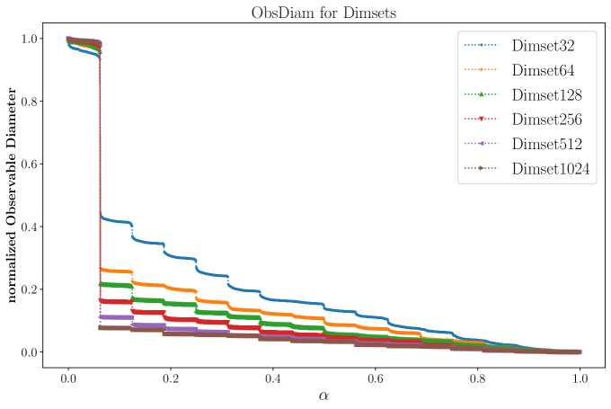
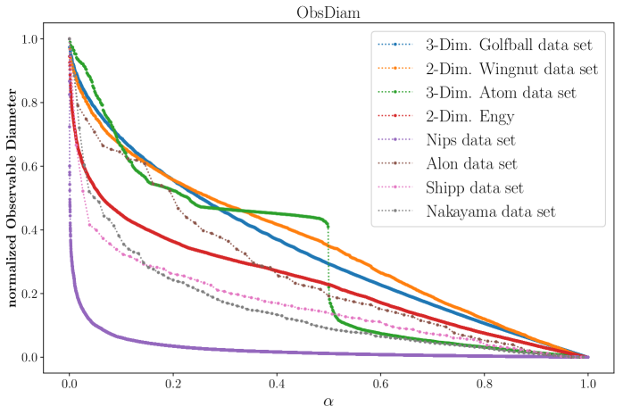
Figure 1. Observable diameter for $\alpha\in[0,1]$ artificial data sets dimset (top) and data sets from [30] (bottom).

Since all dimset data sets were generated using the same procedure with the same number of point samples (1024) one would expect this increase. This is not a mere correlation to the increase in the number of dimensions, but evidence for the inability of the particular generation process to bound the intrinsic dimension. As for the low dimensional artificial data sets we observe a different interaction between the CID an the ID. For example, the CID does decrease when comparing the Golfball data set with the Atom data set, whereas the intrinsic dimension increases. This indicates that the different dimension functions cover different data set properties.

Finally, we compare the results for the real-world data sets. Even though the number of dimensions is quite large, for those we may point out that the number of point samples is quite small, in comparison. Nonetheless, all data sets have essentially enough points to possibly span subspaces of 62 (Alon), 58 (Shippi), and 105 (Nakayama) dimensions. We observe again that an increase in CID does not precede an decrease in ID, as seen for Alon and Shippi. The converse, however, can be observed as well when comparing Alon with Nakayama. The NIPS data set exhibits by far the lowest CID as well as the highest ID. All these observations lead us to conclude that the notion for intrinsic dimension, as introduced in this work, captures an aspect of geometric data sets which is qualitatively different to the Chavez intrinsic dimension.

A.2. Experiments: Incidence Geometries

Table 2. Intrinsic dimension for various data sets and their randomized counterparts.

Name	# Objects	# Attributes	Density	# Concepts	$\partial_{\Delta}(\mathscr{D}(\mathbb{K}))$
zoo	101	28	0.30	379	52.44
zoor	101	28	0.30	3339	1564.40
cancer	699	92	0.10	9862	614.35
cancerr	699	92	0.10	23151	417718.62
southern	18	14	0.35	65	54.93
southernr	18	14	0.37	120	167.01
aplnm	79	188	0.06	1096	11667.14
aplnmr	79	188	0.06	762	185324.01
club	25	15	0.25	62	118.15
clubr	25	15	0.25	85	334.62
facebooklike	377	522	0.01	2973	2689436.00
facebookliker	377	522	0.01	1265	5.73E7
mushroom	8124	119	0.19	238710	263.49

We computed the intrinsic dimension function for different real-world data sets to provide a first impression of $\partial_{\Delta}(\mathscr{D}(\mathbb{K}))$. For brevity we reuse data sets investigated by [5] and refer the reader there for an elaborate discussion of those. All but one of the data sets are scaled versions of downloads from the UCI Machine Learning Repository [15]. In short we will consider the Zoo data set (zoo) describing 101 animals by fifteen attributes. The Breast Cancer data set (cancer) representing 699 clinical cases of cell classification. The Southern Woman data set (southern), a (offline) social network consisting of fourteen woman attending eighteen different events. The Brunson Club Membership Network data set (club), another (offline) social network describing the affiliations of a set of 25 corporate executive officers to a set of 40 social organizations. The Facebook-like Forum Network data set (facebooklike), a (online) social network from an online community linking 377 users to 522 topics. A data set from an annual cultural event organized in the city of Munich in 2013, the so-called Lange Nacht der Musik (aplnm), a (online/offline) social network linking 79 users to 188 events. And, finally the well-known Mushroom data set, a collection of 8124 described by 119 attributes. Additionally we consider for all those data sets, with exception for mushroom, a randomized version. Those are indicated by the suffix r. We conducted our experiments straightforward applying Proposition 6.2. This was done using conexp-clj. The intermediate results for $\mathrm{ObsDiam}$ can be seen in Figures 2 and 3 and the final result for $\partial_{\Delta}(\mathscr{D}(\mathbb{K}))$ is denoted in Table 2.

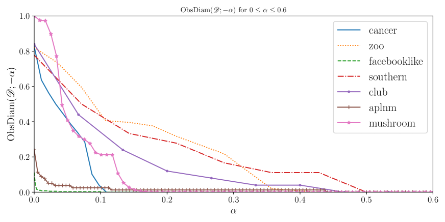
Figure 2. $\mathrm{ObsDiam}$ for all considered real-world data sets.

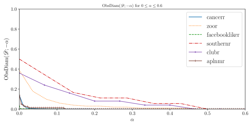
Figure 3. $\mathrm{ObsDiam}$ for randomized data sets based on Figure 2.

A.2.1. Observations

All curves in Figure 2 show a different behavior resulting in different values for $\partial_{\Delta}(\mathscr{D})$. The overall descending monotonicity is expected, however, the average as well as the local slopes are quite distinguished. The general trend that comparably sparse contexts receive a higher intrinsic dimension is also expected taking the results for the empty context into account as well as the overall motivation of the curse of dimension. Considering the random data sets in Table 2 we observe that neither the density nor the number of formal concepts (features) is an indicator for the intrinsic dimension. This suggests that introduced intrinsic dimension is independent of the usual descriptive properties. Comparing these results to the Chavez ID is not applicable due to the non-metric nature of the investigated data sets.

Appendix B Algorithms

Algorithm 1 $\mathrm{ObsDiam}$ with distance features

⬇

1 for $f$ in $F$:

2 $V_{f}=\{\}$

3 Measure ={:} ;dictionary for measures

4 for $x$ in $X$:

5 $V_{f}=V_{f}\cup\{f(x)\}$

6 Measure[$f(x)$] =+ 1 ;preimage measure increase

7 matrix[f,:] = MinDiamMatrix($V_{f}$,Measure,X)

8 for $\alpha$ in $(0,1/|X|,\ldots,(|X|-1)/|X|,1)$

9 result[$\alpha$]=$\max($matrix[:,$\alpha$]$)$

10 return result

Algorithm 2 MinDiamMatrix with distance features

⬇

1 result = $(\operatorname{diam}(X),\ldots,\operatorname{diam}(X))$ ;Initialize vector with length $|X|$

2 for s in $(V_{f},\leq)$: ;iterate through $V_{f}$

3 my_of_x = Measure[s] $\cdot|X|$ ;denormalization to get index

4 diam_of_x = 0

5 if result[my_of_x] > diam_of_x then result[my_of_x] = diam_of_x

6 for e in $\{d\in V_{f}\mid d\geq s\}\leq V_{f}$

7 my_of_x =+ Measure[e] $\cdot|X|$

8 diam_of_x = e - s

9 if result[my_of_x] > diam_of_x then

10 result[my_of_x] = diam_of_x

11 for i in $(|X|,|X|-1,\ldots,1)$: ;repair monotonicity if necessary

12 if result[i] < result[i - 1] then result[i - 1] = result[i]

13 return result

finalnamedelim and

References

• [1] U. Alon et al. “Broad patterns of gene expression revealed by clustering analysis of tumor and normal colon tissues probed by oligonucleotide arrays” In Proceedings of the National Academy of Sciences 96.12, 1999, pp. 6745–6750
• [2] Itaï Ben Yaacov “Lipschitz functions on topometric spaces” In J. Log. Anal. 5, 2013, pp. 21
• [3] Kevin Beyer, Jonathan Goldstein, Raghu Ramakrishnan and Uri Shaft “When Is “Nearest Neighbor” Meaningful?” In Database Theory — ICDT’99 Berlin, Heidelberg: Springer Berlin Heidelberg, 1999, pp. 217–235
• [4] Andrew J. Blumberg, Prithwish Bhaumik and Stephen G. Walker “Testing to distinguish measures on metric spaces” cite arxiv:1802.01152, 2018 URL: http://arxiv.org/abs/1802.01152
• [5] D. Borchmann and T. Hanika “Individuality in Social Networks” In Formal Concept Analysis of Social Networks Cham: Springer International Publishing, 2017, pp. 19–40
• [6] Edgar Chávez, Gonzalo Navarro, Ricardo Baeza-Yates and José Luis Marroquín “Searching in Metric Spaces” In ACM Comput. Surv. 33.3 New York, NY, USA: ACM, 2001, pp. 273–321
• [7] P. Fränti, O. Virmajoki and V. Hautamäki “Fast agglomerative clustering using a k-nearest neighbor graph” In IEEE Trans. on Pattern Analysis and Machine Intelligence 28.11, 2006, pp. 1875–1881
• [8] B. Ganter and R. Wille “Formal Concept Analysis: Mathematical Foundations” Springer-Verlag, Berlin, 1999, pp. x+284
• [9] M. Gromov “Metric structures for Riemannian and non-Riemannian spaces. Transl. from the French by Sean Michael Bates. With appendices by M. Katz, P. Pansu, and S. Semmes. Edited by J. LaFontaine and P. Pansu.” Boston, MA: Birkhäuser, 1999, pp. xix + 585
• [10] M. Gromov and V. D. Milman “A Topological Application of the Isoperimetric Inequality” In American Journal of Mathematics 105.4 Johns Hopkins University Press, 1983, pp. 843–854
• [11] Michael E. Houle et al. “Can Shared-Neighbor Distances Defeat the Curse of Dimensionality?” In SSDBM 6187, Lecture Notes in Computer Science Springer, 2010, pp. 482–500
• [12] A.S. Kechris “Classical Descriptive Set Theory”, Graduate Texts in Mathematics 156 Springer-Verlag, 1995
• [13] John L. Kelley “General topology” Reprint of the 1955 edition [Van Nostrand, Toronto, Ont.], Graduate Texts in Mathematics, No. 27 Springer-Verlag, New York-Berlin, 1975, pp. xiv+298
• [14] F. Korn, B. U. Pagel and C. Faloutsos “On the ”dimensionality curse” and the ”self-similarity blessing”” In IEEE Transactions on Knowledge and Data Engineering 13.1, 2001, pp. 96–111
• [15] M. Lichman “UCI Machine Learning Repository”, 2013 URL: http://archive.ics.uci.edu/ml
• [16] V. D. Milman “The heritage of P. Lévy in geometrical functional analysis” Colloque Paul Lévy sur les Processus Stochastiques (Palaiseau, 1987) In Astérisque, 1988, pp. 273–301
• [17] V. D. Milman “Topics in Asymptotic Geometric Analysis” In Visions in Mathematics: GAFA 2000 Special volume, Part II Basel: Birkhäuser Basel, 2010, pp. 792–815
• [18] Robert Nakayama et al. “Gene expression analysis of soft tissue sarcomas: characterization and reclassification of malignant fibrous histiocytoma” In Nature 20.7, 2007, pp. 749–759
• [19] Ryunosuke Ozawa and Takashi Shioya “Estimate of observable diameter of $l_{p}$-product spaces” In Manuscripta Math. 147.3-4, 2015, pp. 501–509
• [20] Jan Pachl “Uniform spaces and measures.” In Fields Inst. Monogr. 30 New York, NY: Springer; Toronto: The Fields Institute for Research in the Mathematical Sciences, 2013, pp. ix + 209
• [21] K. R. Parthasarathy “Probability measures on metric spaces”, Probability and Mathematical Statistics, No. 3 Academic Press, Inc., New York-London, 1967, pp. xi+276
• [22] Valerio Perrone, Paul A. Jenkins, Dario Spanò and Yee Whye Teh “Poisson Random Fields for Dynamic Feature Models.” In Journal of Machine Learning Research 18, 2017, pp. Paper No. 127, 45 pp.
• [23] Vladimir Pestov “An axiomatic approach to intrinsic dimension of a dataset” In Neural Networks 21.2-3, 2008, pp. 204–213
• [24] Vladimir Pestov “Dynamics of infinite-dimensional groups” The Ramsey-Dvoretzky-Milman phenomenon, Revised edition of ıt Dynamics of infinite-dimensional groups and Ramsey-type phenomena [Inst. Mat. Pura. Apl. (IMPA), Rio de Janeiro, 2005; MR2164572] 40, University Lecture Series American Mathematical Society, Providence, RI, 2006, pp. viii+192
• [25] Vladimir Pestov “Intrinsic dimension of a dataset: what properties does one expect?” In Proceedings of the International Joint Conference on Neural Networks, IJCNN 2007, Celebrating 20 years of neural networks, Orlando, Florida, USA, August 12-17, 2007, 2007, pp. 2959–2964
• [26] Vladimir Pestov “On the geometry of similarity search: Dimensionality curse and concentration of measure” In Inf. Process. Lett. 73.1-2, 2000, pp. 47–51
• [27] T. Shioya “Metric Measure Geometry: Gromov’s Theory of Convergence and Concentration of Metrics and Measures”, IRMA Lectures in Mathematics and Theoretical Physics 25 European Mathematical Society, 2016
• [28] Takashi Shioya “Metric measure limits of spheres and complex projective spaces” In Measure theory in non-smooth spaces, Partial Differ. Equ. Meas. Theory De Gruyter Open, Warsaw, 2017, pp. 261–287
• [29] Margaret A Shipp et al. “Diffuse large B-cell lymphoma outcome prediction by gene-expression profiling and supervised machine learning.” In Nature Medicine 8.1, 2002, pp. 68–74
• [30] Alfred Ultsch “Clustering with SOM: U*C” In Proc. Workshop on Self-Organizing Maps, 2005, pp. 75–82