Circumstellar environment of the M-type AGB star R Dor

Abstract

Context. Our current insights into the circumstellar chemistry of asymptotic giant branch (AGB) stars are largely based on studies of carbon-rich stars and stars with high mass-loss rates.

Aims. In order to expand the current molecular inventory of evolved stars we present a spectral scan of the nearby, oxygen-rich star R Dor, a star with a low mass-loss rate ($\sim 2\times 10^{-7}$ $M_{\sun}$ yr^-1).

Methods. We carried out a spectral scan in the frequency ranges $159.0-321.5$ GHz and $338.5-368.5$ GHz (wavelength range $0.8-1.9$ mm) using the SEPIA/Band-5 and SHeFI instruments on the APEX telescope and we compare it to previous surveys, including one of the oxygen-rich AGB star IK Tau, which has a high mass-loss rate ($\sim 5\times 10^{-6}$ $M_{\sun}$ yr^-1).

Results. The spectrum of R Dor is dominated by emission lines of SO₂ and the different isotopologues of SiO. We also detect CO, H₂O, HCN, CN, PO, PN, SO, and tentatively TiO₂, AlO, and NaCl. Sixteen out of approximately 320 spectral features remain unidentified. Among these is a strong but previously unknown maser at 354.2 GHz, which we suggest could pertain to H₂SiO, silanone. With the exception of one, none of these unidentified lines are found in a similarly sensitive survey of IK Tau performed with the IRAM 30 m telescope. We present radiative transfer models for five isotopologues of SiO (²⁸SiO, ²⁹SiO, ³⁰SiO, Si¹⁷O, Si¹⁸O), providing constraints on their fractional abundance and radial extent. We derive isotopic ratios for C, O, Si, and S and estimate that, based on our results for ¹⁷O/¹⁸O, R Dor likely had an initial mass in the range $1.3-1.6$ $M_{\sun}$, in agreement with earlier findings based on models of H₂O line emission. From the presence of spectral features recurring in many of the measured thermal and maser emission lines we tentatively identify up to five kinematical components in the outflow of R Dor, indicating deviations from a smooth, spherical wind.

Figure 1: APEX survey of R Dor in the range $159.0-368.5$ GHz.

1 Introduction

In order to get a comprehensive view of the physical and chemical properties of the circumstellar envelopes (CSEs) of asymptotic giant branch (AGB) stars and to quantify their return to the interstellar medium, it is necessary to characterise the gas and dust contents of these outflows. The set-up of an inventory of chemical species present in the CSEs of evolved stars has predominantly used, as reference, the nearby, high-mass-loss-rate, carbon-rich AGB star IRC +10 216 (also commonly referred to as CW Leo), skewing the community’s knowledge towards the carbon-rich chemistry, both observationally and theoretically. A similar wealth of observational constraints on the circumstellar chemistry of M-type AGB stars, often called oxygen-rich given their atmospheric C/O$<1$, is currently still lacking.

Unbiased spectral surveys, scanning broad frequency ranges without pre-selecting particular molecules of interest, are excellent tools to set up such inventories. Several such surveys using single-dish telescopes have been presented for high-mass-loss-rate, carbon-rich AGB stars: IRC +10 216 (Cernicharo et al. 2000, 2010), CIT 6 (RW LMi; Zhang et al. 2009a), and CRL 3068 (LL Peg; Zhang et al. 2009b). Patel et al. (2011) presented an interferometric survey of IRC +10 216 obtained with the Submillimeter Array (SMA). Kamiński et al. (2013b) reported on a similar SMA line-imaging survey of the red supergiant VY CMa, a star with an oxygen-rich composition, an extremely high mass-loss rate of several $10^{-4}$ $M_{\sun}$ yr^-1, and a geometrically and chemically complex CSE (e.g. Humphreys et al. 2007; Richards et al. 2014; Ziurys et al. 2007). De Beck et al. (2015a) presented an overview of an interferometric spectral survey of the Mira-type, high-mass-loss-rate, M-type star IK Tau in the range $279-355$ GHz carried out with the SMA. A forthcoming publication (De Beck et al., in prep.) will report on this survey in its entirety, including a discussion on the extent and geometry of the imaged line emission. Based partially on this survey, De Beck et al. (2013) presented first results on phosphorus-bearing molecules in the CSE of an M-type AGB star and highlighted the need for updated chemical models for these CSEs. Velilla Prieto et al. (2017) recently presented a spectral scan of IK Tau obtained with the IRAM 30 m telescope covering the ranges $79-116$, $128-175$, and $202-356$ GHz. They reported a very rich chemical content, including several carbon-bearing molecules, such as H₂CO and HCO⁺, and several nitrogen-bearing molecules, such as NS and NO. The abundances they derive for several of the detected species further underscore the need for improved models of the chemistry around oxygen-rich stars.

We present here for the first time a spectral scan of a low-mass-loss-rate M-type AGB star, R Dor, enabling a direct comparison of the chemical contents of CSEs representative of two significantly different density regimes. R Dor is a nearby (59 pc; Knapp et al. 2003) AGB star with a luminosity of about 6500 $L_{\sun}$ (Maercker et al. 2016). It shows a semi-regular pulsation pattern with two periods of 175 and 332 days, respectively (Bedding & Zijlstra 1998). Studies of its circumstellar environment have mainly focussed on CO and H₂O line emission (e.g. Ramstedt & Olofsson 2014; Maercker et al. 2016), constraining its mass-loss rate to $1-2\times 10^{-7}$ $M_{\sun}$ yr^-1. Recently, Van de Sande et al. (2018) reported on a detailed abundance analysis of SiO and HCN.

We list the details of the observations in Sect. 2, present and discuss the results in Sect. 3, and provide a list of unidentified spectral features in Sect. 3.4. We compare our results to those obtained from other line surveys, in particular of IK Tau, in Sect. 4, discuss possible deviations in the outflow from spherical symmetry in Sect. 5, and present our conclusions in Sect. 6. Appendix A addresses possible time variability of the CO line emission. Appendix B addresses maser line variability and includes a list of detected masers. Appendix C provides an overview of the full survey.

2 Observations

We used the Swedish Heterodyne Facility Instrument (SHeFI; Vassilev et al. 2008) and band 5 of the Swedish-ESO PI Instrument (SEPIA; Billade et al. 2012) on the Atacama Pathfinder Experiment (APEX) telescope to carry out a spectral survey covering the frequency range $159.0-368.5$ GHz. Due to excessive interference of water vapour in the atmosphere the survey does not cover the range $321.5-328.0$ GHz. The SHeFI observations were carried out over a long period, spanning from May 2011 up to November 2015. All SEPIA observations were carried out on 22 and 23 November, 2015.

SHeFI is a single-sideband (sideband-separating), single-polarisation heterodyne receiver, whereas SEPIA is a sideband-separating, dual-polarisation heterodyne receiver. The backends for SHeFI changed during the observing campaign and were extended from an initial $2\times 1.0$ GHz bandwidth (FFTS) to $2\times 2.5$ GHz (XFFTS), corresponding to instantaneous bandwidths of 1.9 GHz and 4.0 GHz, respectively, significantly increasing the observing efficiency. The SEPIA backends consist of $2\times 2\times 2\times 2.5$ GHz, covering both lower and upper sidebands simultaneously, in two polarisations. The SHeFI spectra were recorded at a nominal resolution of 122 kHz when the FFTS was used, and at 76 kHz when the XFFTS was used. The SEPIA spectra were recorded at 38 kHz nominal resolution. Consecutive tunings were separated by 1.5 GHz or 3.5 GHz, depending on the backend in use, to ensure sufficient overlap.

The observations were carried out using wobbler switching with a standard beam throw of 50″. Due to some technical issues with the wobbler, some settings were observed in position switching mode, without compromising the final result. The main beam half power beamwidth of APEX varies in the range $17-39$″ over the observed frequency range.

Data reduction is done using the gildas/class package. We inspect scans individually and ignore those with very unstable baselines. Bad channels, which commonly appear in the outer $30-50$ MHz of the band are blanked. We subtract first-degree polynomial baselines from the individual scans, after masking relevant spectral features, and combine all data into one final spectrum.

In a few cases, we find aliases of strong lines of CO and SiO, in the outer $\sim 60$ MHz of the receiver backend. These can occur when the strong signal is very close to the edge of the XXFTS unit and gets folded into the band. Given the proximity to the band edge, and the overlapping observing settings, these aliases are removed from the spectra without losing spectral coverage.

The SHeFI receivers on APEX work in single-sideband mode with reported image-sideband suppression of typically $>15$ dB. The sideband-separating SEPIA instrument has an average image-sideband suppression of $18.5$ dB. Some strong lines can, therefore, leak into the one sideband from the other for some frequency settings. In case there is no overlapping spectral coverage from another frequency tuning available, we do not blank these lines in our spectrum, but clearly mark these leakages in the overview tables and plots. The leakage levels in our survey range from 0.3% (25 dB suppression of an 11 K strong signal) up to 54% (3 dB) in the most extreme case, but are overall well in line with the reported suppression values.

We assume overall calibration uncertainties of 20% on the survey data, but argue in Sect. 3.2.2 that the internal uncertainties, that is, line-to-line uncertainties, are most likely lower than that.

Unless stated otherwise, we show all spectra in $T_{\mathrm{A}}^{*}$, that is, the antenna temperature scale corrected for atmospheric losses and, for example, antenna spillover. Typical rms noise values on this scale vary from 3 mK to 10 mK at 2 km s^-1 resolution, with higher rms locally induced by the interference of atmospheric H₂O at 183 GHz and 321 GHz. For conversion into flux units one can employ point-source sensitivities $S_{\nu}/T_{\rm A}^{*}$ of 38 Jy/K, 39 Jy/K, and 41 Jy/K for the SEPIA/band-5 ($159-211$ GHz), SHeFI-1 ($213-275$ GHz), and SHeFI-2 ($267-378$ GHz) observations, respectively. Conversion to main-beam brightness temperature, $T_{\rm mb}=T_{\mathrm{A}}^{*}/\eta_{\rm mb}$, used in this work for comparison to modelling results, uses main-beam efficiencies $\eta_{\rm mb}$ of 0.68, 0.75, and 0.73 for the different bands, respectively. The values for SEPIA/band-5 are preliminary, but currently the most up-to-date (Immer et al. 2016).

We claim detection of a spectral feature at signal-to-noise ratios (S/Ns) of at least 3 at a spectral resolution that leaves a minimum of five spectral bins covering the line. Additionally, tentative detections of lines at low S/N can be claimed in the case where a stacked spectrum reaches this S/N criterion (e.g. for PN, see below) or if one, or more, other emission lines of the same molecule are present elsewhere in the spectrum.

3 Results

Figure 1 shows a low-resolution overview of the APEX line survey of R Dor. Figure 25 in the appendix shows the entire survey at 3 MHz frequency resolution. Table LABEL:tbl:lineID gives an overview of all emission features in the scan, while Table 1 gives an overview of the identified lines per molecule. The spectrum is dominated by emission lines of SO₂ (134 lines), SiO (50 lines), and SO (28 lines), including isotopologues.

For line identification we use the Cologne Database for Molecular Spectroscopy (CDMS; Müller et al. 2001, 2005) and the catalogue for molecular line spectroscopy hosted by the Jet Propulsion Laboratory (JPL; Pickett et al. 1998) as primary reference catalogues, with priority given to CDMS when entries are present in both.

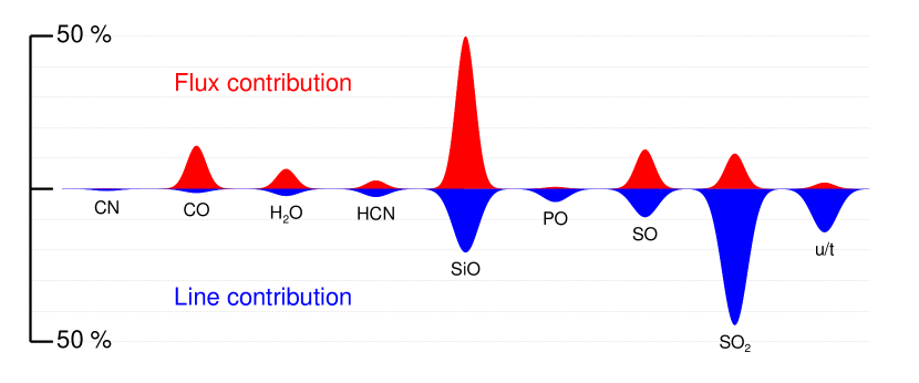
Figure 2: Overview of the relative contribution per molecule (including isotopologues) to the survey in terms of flux (top) and number of lines (bottom). Unidentified and tentatively identified spectral features are grouped under the label “u/t”.

Table 1: Overview of molecules in the APEX survey of R Dor.

Molecule	Number	Line numbers
	of lines
CN	2	268, 270
CO	2	86, 289
13CO	2	80, 243
H2O	2	37, 239
H2O, $v_{2}=1$	5	87, 141, 192, 202, 256
H2O, $v_{2}=2$	1	149
HCN	3	34, 144, 303
H13CN	3	27, 134, 286
PO	12	48, 49, 50, 51, 94, 95, 96, 97, 173, 174, 175, 176
SiO	5	29, 78, 136, 220, 295
SiO, $v=1$	5	26, 75, 132, 216, 284
SiO, $v=2$	3	22, 127, 212
SiO, $v=3$	4	20, 68, 203, 269
SiO, $v=5$	1	115
29SiO	5	23, 71, 129, 213, 280
29SiO, $v=1$	4	21, 123, 205, 272
29SiO, $v=2$	2	120, 262
29SiO, $v=3$	2	193, 254
30SiO	5	19, 67, 121, 200, 265
30SiO, $v=1$	3	18, 118, 257
Si17O	5	16, 65, 112, 190, 251
Si18O	5	5, 56, 100, 169, 331
29Si18O	1	161
SO	16	25, 36, 63, 74, 79, 117, 130, 138, 199, 215, 221, 226, 266, 273, 281, 293
34SO	12	32, 57, 76, 108, 119, 126, 195, 206, 250, 260, 267, 306
SO2	116	1, 4, 9, 11, 13, 14, 31, 43, 45, 46, 47, 52, 54, 55, 58, 60, 61, 64, 69, 72, 77, 81, 82, 83, 85, 88, 90, 91, 92, 98, 99, 102, 105, 106, 109, 111, 113, 114, 122, 124, 125, 128, 131, 133, 135, 140, 142, 145, 146, 152, 157, 158, 163, 164, 165, 167, 168, 171, 179, 186, 197, 198, 208, 211, 214, 217, 223, 227, 228, 229, 230, 231, 235, 236, 240, 244, 248, 252, 255, 258, 263, 264, 271, 274, 275, 276, 277, 279, 285, 292, 294, 296, 298, 299, 304, 305, 309, 311, 312, 313, 315, 316, 317, 318, 319, 320, 321, 323, 325, 327, 328, 329, 332, 333, 334, 336
SO2, $v_{2}=1$	1	297
34SO2	5	7, 30, 104, 310, 330
SO17O	2	233, 290
SO18O	9	177, 178, 183, 184, 185, 218, 219, 283, 291
u	16	28, 44, 59, 84, 148, 156, 162, 172, 196, 201, 207, 225, 234, 237, 245, 302

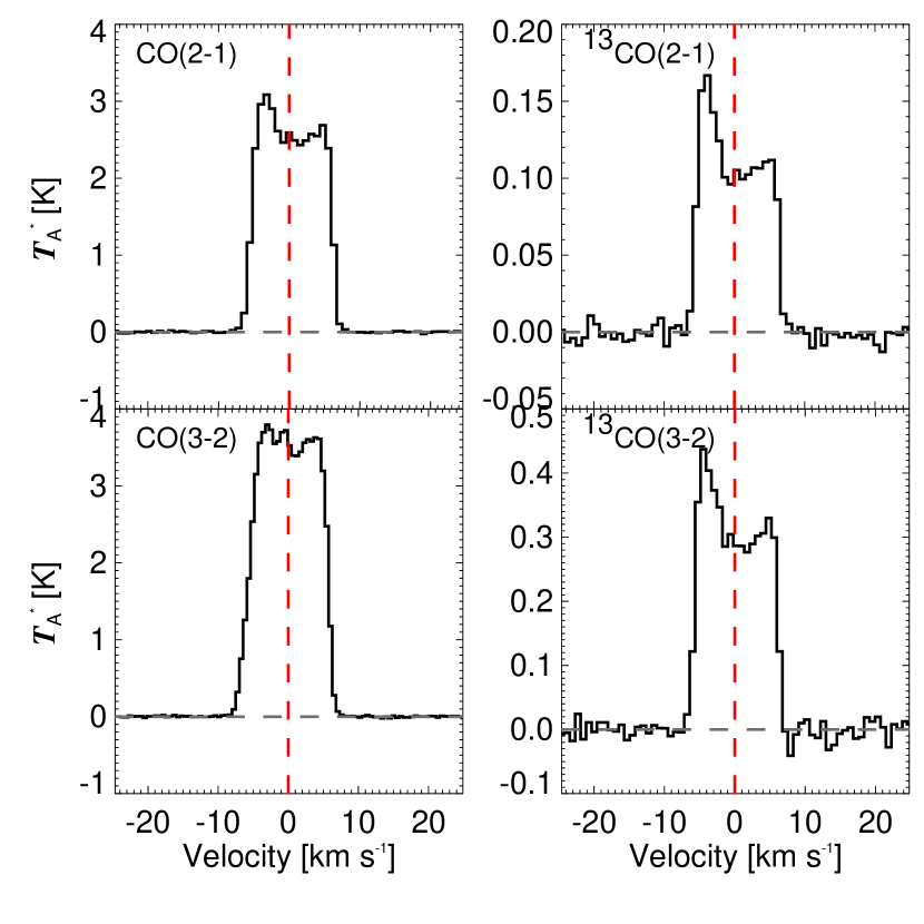
Figure 3: CO line emission. Left: ¹²CO, right: ¹³CO.

3.1 Molecular line luminosity

The molecular line emission observed in the survey is dominated by only a few molecules. Approximately 50% of the total line flux comes from SiO and its isotopologues, which accounts for 21% of the emission features. Another 14% of the flux comes from the four (1.3%) CO lines. SO accounts for 13% of the flux and 9% of the lines. SO₂ accounts for another 12% of the flux and 45% of the lines. H₂O accounts for 6% of the flux and 2% of the lines. Other species each contribute less than 3% of the total flux. Figure 2 presents a visual summary of this.

3.2 Molecular species

Throughout the paper, we assume that the source’s systemic velocity, $\varv_{\mathrm{LSR}}$, is 6.5 km s^-1, and plot profiles with respect to the stellar $\varv_{\mathrm{LSR}}$, that is, centered around 0.0 km s^-1. This value for the systemic velocity corresponds to individual peaks in, for example, the CO lines, the 321 GHz H₂O maser, and many of the SO₂ lines already presented by Danilovich et al. (2016). It also matches the central depression in the 183 GHz H₂O maser and appears appropriate based on, for example, the selection of emission features pertaining to different molecules and spanning a large range of excitation conditions as discussed in Sect. 5. Finally, it is also in agreement with the radiative-transfer modelling efforts from earlier publications (e.g. Maercker et al. 2016).

3.2.1 Carbon monoxide

The estimated radial extent of the CO envelope of R Dor, that is, the $e$-folding radius of the CO abundance profile, is $1.6\times 10^{16}$ cm, corresponding to an angular (diametric) size of 36″ at a distance of 59 pc (Maercker et al. 2016). The ¹²CO and ¹³CO emission lines measured towards R Dor in this survey are hence slightly spatially resolved (see e.g. Fig. 21) and the spectra do not recover all of the emission as these are single-pointing observations. On the contrary, for all the other molecular line emissions the loss of flux is estimated to be small.

Our observations of the ¹²CO($J=2-1,3-2$) and ¹³CO($J=2-1,3-2$) line emission (Fig. 3) agree within 15% (in intensity) with the independently performed APEX observations of Ramstedt & Olofsson (2014). We discuss possible variability over time of the CO line emission in App. A. We refer to Ramstedt & Olofsson (2014) and Maercker et al. (2016) for detailed radiative transfer models of CO.

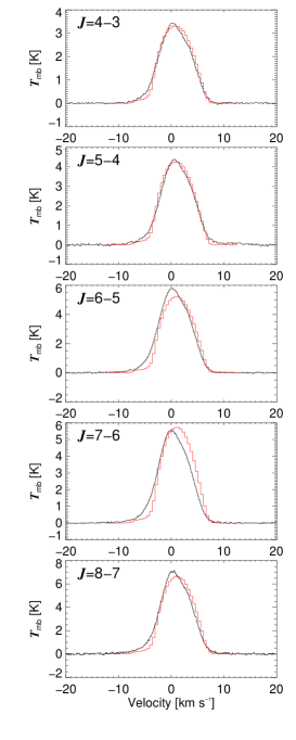
(a) ²⁸Si¹⁶O

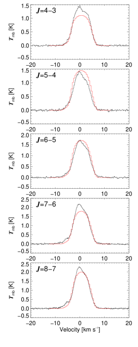
(b) ²⁹Si¹⁶O

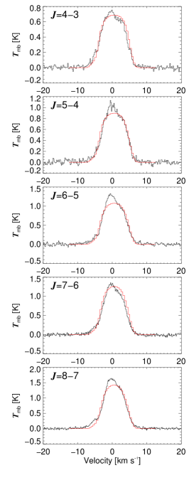
(c) ³⁰Si¹⁶O

Figure 4: SiO isotopologue (^28,29,30Si¹⁶O) $v=0$ line emission (black) and the predictions from our best-fit radiative transfer models (red). We note that the line intensity is given as main-beam brightness temperature $T_{\rm mb}$.

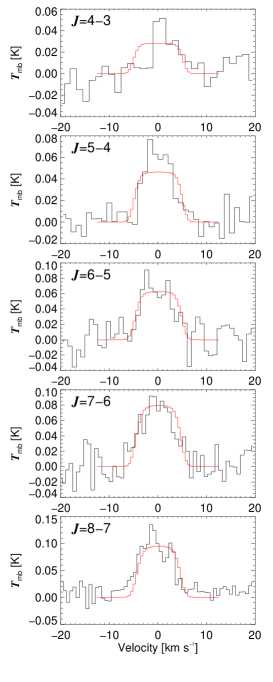
(a) ²⁸Si¹⁷O

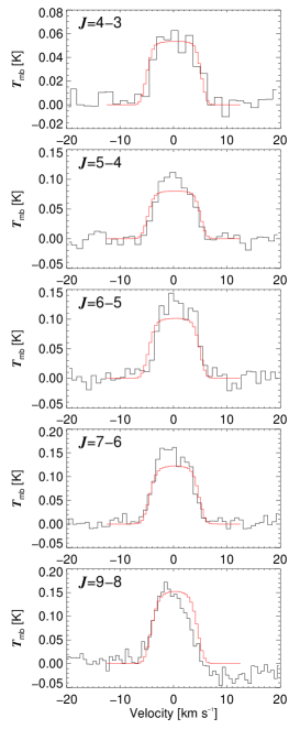
(b) ²⁸Si¹⁸O

Figure 5: SiO isotopologue (²⁸Si^17,18O) $v=0$ line emission (black) and the predictions from our best-fit radiative transfer models (red). We note that the line intensity is given as main-beam brightness temperature $T_{\rm MB}$.

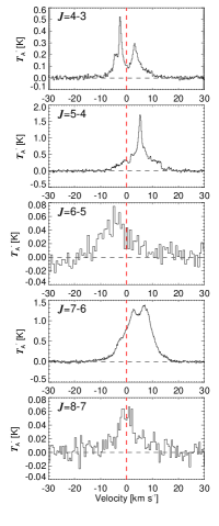
(a) ²⁸Si¹⁶O

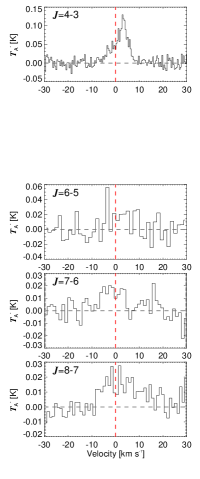
(b) ²⁹Si¹⁶O

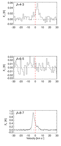
(c) ³⁰Si¹⁶O

Figure 6: SiO isotopologue $v=1$ line emission. We point out that the ³⁰SiO ($v=1,J=8-7$) emission is blended with emission from SO₂ ($v_{2}=1,J_{K_{\rm a},K_{\rm c}}=6_{5,1}-7_{4,4}$) centred at $\sim$3 km s^-1 in the rest frame of the SiO line.

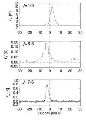
(a) ²⁸Si¹⁶O

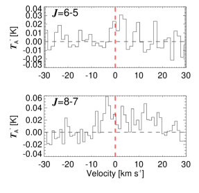
(b) ²⁹Si¹⁶O

Figure 7: SiO isotopologue $v=2$ line emission.

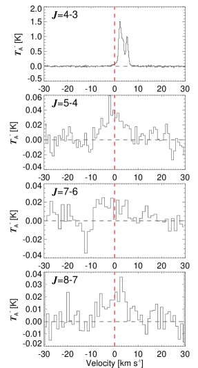
(a) $v=3$

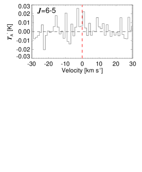
(b) $v=5$

Figure 8: ²⁸Si¹⁶O line emission in higher excited states.

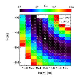
(a) ²⁸SiO

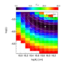
(b) ²⁹SiO

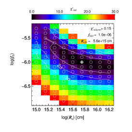
(c) ³⁰SiO

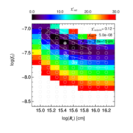
(d) ²⁸Si¹⁷O

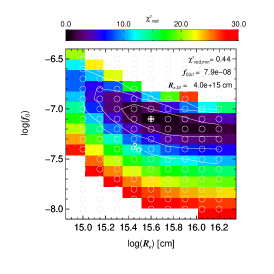
(e) ²⁸Si¹⁸O

Figure 9: Reduced-$\chi^{2}$ maps of the model grids for the $v=0$ state of five SiO isotopologues. Circles indicate the grid points and white crosses indicate the best-fit models. Contours are given at the $\sim$68%, $\sim$95%, and 99.7% confidence intervals ($1\sigma,2\sigma,3\sigma$, resp.).

3.2.2 Silicon monoxide

We detect 50 transitions of SiO and its isotopologues. Figures 4 to 8 show the spectra for the transitions $J=4-3,...,9-8$ in the vibrational states $v=0,...,5$ for the isotopologues ²⁸SiO, ²⁹SiO, ³⁰SiO, Si¹⁷O, and Si¹⁸O. The intensity-weighted mean velocity of the lines (in $v=0$) of the different isotopologues shifts slightly to the red with increasing $J$. This could be explained by an increasing optical thickness that causes stronger self-absorption in the blue wing with increasing $J$, shifting the peak of the emission redwards. This effect is reproduced by our radiative transfer models discussed below.

Emission in transitions in the vibrational ground state ($v=0$) is most often assumed to be of non-maser nature. However, recently, de Vicente et al. (2016) showed that the SiO($v=0,J=1-0$) transition exhibits clear (and variable) signatures of maser nature in many of the oxygen-rich and S-type AGB stars in their sample. These maser components are thought to be excited in the very inner layers of the CSE, where no dust is present yet. de Vicente et al. (2016) further state that higher-$J$ transitions are typically of thermal nature. We note, however, that time-variable features are occasionally seen in the $J=2-1$ emission and that these are likely of maser nature, see Nyman & Olofsson (1985). Judging from the appearance of the emission features in this survey and in the HIFI data (Fig. 21; $J=4-3$ and higher) thermal excitation indeed seems to be likely for the observed $v=0$ lines.

Table 2: Radiative transfer modelling results for SiO isotopologues.

Isotopologue	$\log(f_{0})$			$\log(R_{e}[\mathrm{cm}])$
	Grid range (step)	Best-fit value	$1\sigma$-range	Grid range (step)	Best-fit value	$1\sigma$-range
28Si16O	$[-5.5,-4.0]$ (0.1)	-4.7	$[-5.2,-4.0]$	$[15.00,16.20]$ (0.15)	15.60	$[15.15,16.20]$
29Si16O	$[-6.8,-5.3]$ (0.1)	-5.8	$[-5.9,-5.4]$	$[15.00,16.20]$ (0.15)	15.90	$[15.30,16.20]$
30Si16O	$[-6.8,-5.3]$ (0.1)	-6.0	$[-6.2,-5.5]$	$[15.00,16.20]$ (0.15)	15.75	$[15.15,16.20]$
28Si17O	$[-8.5,-7.0]$ (0.1)	-7.3	$[-7.5,-7.1]$	$[15.00,16.20]$ (0.15)	15.45	$[15.15,15.90]$
28Si18O	$[-8.0,-6.5]$ (0.1)	-7.1	$[-7.2,-7.0]$	$[15.00,16.20]$ (0.15)	15.60	$[15.45,16.20]$

For vibrationally excited states ($v\neq 0$) the emission is clearly of maser nature, often with multiple peaks in the line profiles. These complex shapes are furthermore not constant across the excitation ladder within one vibrational state. We plot a selection of the highest-S/N maser lines of SiO (any isotopologue) in Fig. 22. As mentioned before, several of the individual maser peaks correspond to the velocities where peaks or bumps also appear in thermal emission lines. Overall, it is clear that the SiO maser emission can differ substantially between different transitions, even within the same vibrationally excited state of a given isotopologue. Some maser lines are composed of several peaks over the entire velocity range (e.g. ²⁸SiO($v=1,J=4-3$)), some are limited to only blue or red-shifted velocities (e.g. ²⁸SiO($v=3,J=4-3$) and ²⁸SiO($v=2,J=7-6$)), and some appear as very broad emission lines with barely discernible maser components (e.g. ²⁸SiO($v=1,J=7-6$)). This is in line with both observations and simulations of SiO masers in the CSEs of red giant and supergiant stars (e.g. Humphreys et al. 1997, 2002; Desmurs et al. 2014), from which it is apparent that the excitation of different rotational transitions within the same vibrational state is not necessarily co-spatial. This, in combination with non-simultaneity of the observations, explains the variety in the profiles we observe towards R Dor. We therefore add Table 5 listing the observing dates of these lines in App. B.

The wealth of emission lines from different SiO isotopologues, spanning the entire frequency range of the survey, motivates a deeper investigation through modelling. We base the radiative transfer modelling of the SiO $v=0$ line emission on the CSE model reported by Maercker et al. (2016). Our molecular input covers the rotational levels for $J=0,\dots,40$ of the $v=0,1$ states of ²⁸SiO, ²⁹SiO, ³⁰SiO, Si¹⁷O, and Si¹⁸O. Collisional rates are included for SiO–H₂, adapted from the collisional rates for SiO–He of Dayou & Balança (2006). The modelling is performed using the accelerated lambda iteration (ALI) radiative transfer code described and implemented by Maercker et al. (2008, 2016); Danilovich et al. (2014).

We assume a centrally peaked Gaussian fractional abundance distribution

$$f(r)=f_{0}\exp\left(-\left(\frac{r}{R_{e}}\right)^{2}\right),$$ (1)

with $f_{0}$ the molecular abundance (w.r.t. H₂) at the inner radius of the CSE (at 5 $R_{\star}$, following Danilovich et al. 2016), also referred to as peak abundance in the rest of the paper, and $R_{e}$ the $e$-folding radius of the Gaussian profile. We set up a model grid for these two free parameters, $f_{0}$ and $R_{e}$, as summarised in Table 2. We minimise the reduced-$\chi^{2}$

$$\chi^{2}_{\mathrm{red}}=\frac{1}{N-p}\sum_{i=1}^{N}\left(\frac{I_{\mathrm{mod}}-I_{\mathrm{obs}}}{\sigma}\right)^{2},$$ (2)

with $N$ being the number of modelled transitions (five for each isotopologue), $p$ the number of free parameters (two), $I_{\mathrm{mod}}$ and $I_{\mathrm{obs}}$ the modelled and observed integrated line intensities, respectively, and $\sigma$ the uncertainty on $I_{\mathrm{obs}}$. We assume uncertainties on the data at a 20% level, accounting for predominantly the calibration uncertainties, given the high S/Ns in the modelled lines. Table 2 lists the best-fit values of $f_{0}$ and $R_{e}$ with their $1\sigma$-uncertainties for each of the isotopologues. We show the reduced-$\chi^{2}$ maps in Fig. 9 and the comparison of the best-fit models to the survey data in Figs. 4 and 5. In general, we find that there is a rather large degeneracy in the radiative transfer modelling between the two free parameters, $f_{0}$ and $R_{e}$, visible as the elongated $1\sigma$-confidence intervals. This degeneracy is most significant for the main isotopologue, ²⁸Si¹⁶O, where abundances in the range $0.6-10\times 10^{-5}$ can reproduce the emission to within the uncertainties, according to the very clear trend that a lower $f_{0}$ requires a larger $R_{e}$ (Fig. 9(a)). This is a consequence of the high optical depth involved in the radiative transfer of this molecule. Natural upper limits to $R_{e}$ and $f_{0}$ can in this case be set by the size of the CO envelope and the Si abundance (${\rm Si/H}\approx 3.2\times 10^{-5}$; Asplund et al. 2009) which implies ${\rm SiO/H}_{2}\lesssim 6.4\times 10^{-5}$ or $\log\left({\rm SiO/H}_{2}\right)\lesssim-4.2$ if all silicon is comprised in SiO and all H is in molecular form.

González Delgado et al. (2003) and Schöier et al. (2004) modelled thermal SiO emission ($J=2-1,3-2,5-4,6-5$) from the CSE of R Dor. More recently, Van de Sande et al. (2018) additionally modelled several high-$J$ transitions (up to $J=38-37$). Based on interferometric observations of SiO ($J=2-1$), Schöier et al. (2004) found that the SiO abundance profile of R Dor is possibly better represented by a compact component with a high, constant, abundance of $4\times 10^{-5}$ out to $r=1.2\times 10^{15}$ cm and a component with a low abundance ($3\times 10^{-6}$ and declining according to a Gaussian profile) at larger radii. The discontinuity in the abundance is thought to reflect the signature of depletion of SiO onto dust. Since we restrict our modelling to higher-excitation transitions, ignoring the possible depletion signature as derived by Schöier et al. (2004) is not expected to pose a problem. Our best-fit value of $f_{0}$ falls in between those of the previous models and our uncertainties cover both the low-lying values of González Delgado et al. (2003) and Schöier et al. (2004) and the high $f_{0}$ found by Van de Sande et al. (2018). The range of acceptable values of $R_{e}$ we find is also in agreement with the results of both González Delgado et al. (2003); Schöier et al. (2004) and Van de Sande et al. (2018, as presented in their Fig. 6).

We are not aware of any earlier efforts to model the thermal emission of the less abundant isotopologues ²⁹SiO, ³⁰SiO, Si¹⁷O, and Si¹⁸O, except for the modelling by Decin et al. (2010) of two ²⁹SiO transitions measured towards IK Tau. We set up our model grids based on the one for ²⁸SiO, covering the same values for $R_{e}$ and scaling those for $f_{0}$ with a reasonable value for the appropriate isotopic ratio. See Table 2 for the grid specifications and model results. Figures 4 and 5 show that our model predictions reproduce the observed data very well. We note that the remarkable quality of the fit to all emission lines simultaneously, for each of the modelled isotopologues, demonstrates that the survey’s internal data calibration uncertainty is actually (significantly) lower than the 20% we quote as absolute uncertainty in Sect. 2. To assess the variability in SiO line emission as a consequence of stellar variability, we calculated a radiative transfer model (for ²⁸SiO) based on our best-fit model, but decreasing the luminosity to 4500 $L_{\sun}$. This significant change in luminosity leads to changes in intensity within 20% and in integrated line intensity within 15% for the observed lines. Such line variability would hence not be significant with respect to the observational uncertainties in the selection of our models.

To obtain isotopologue abundance ratios from these results, we consider all models, that is, combinations of $f_{0}$ and $R_{e}$, that fall within $1\sigma$ of the best-fit model for a given isotopologue. Additionally, assuming that all isotopologues are photodissociated by the interstellar radiation field at the same radius and, hence, have the same $e$-folding radius $R_{e}$, we can reduce the uncertainties on these ratios by only considering the abundance ratios at a given $R_{e}$. This approach leads to the values and uncertainties listed in Table 3 and discussed in Sect. 3.3.

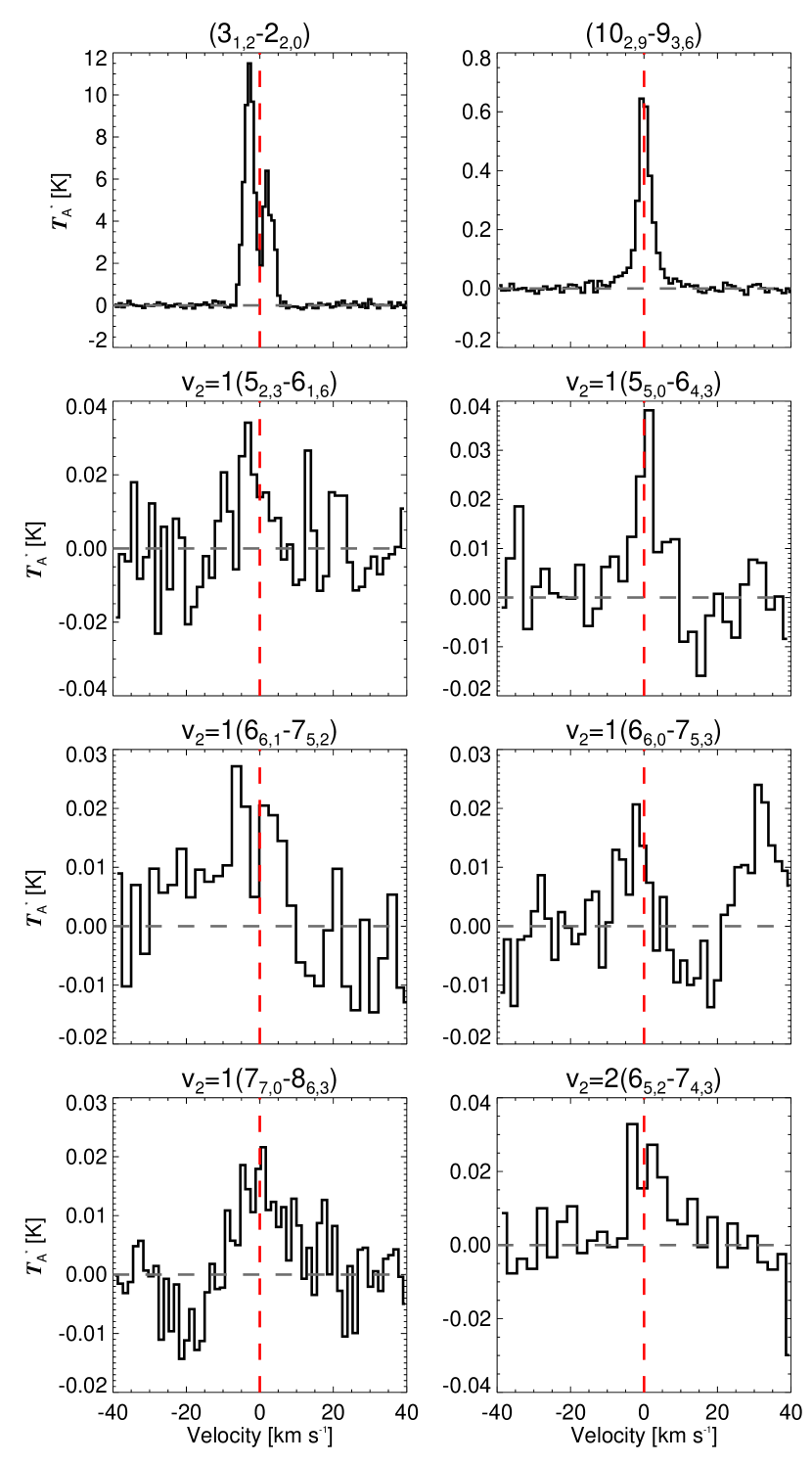
Figure 10: H₂O emission in the vibrational ground state and the vibrationally excited states $v_{2}=1,2$.

3.2.3 Water

We detect eight emission features of H₂O: the well-known masers at 183 GHz and 321 GHz in the vibrational ground state, and five and one lines in the vibrationally excited states $\nu_{2}$ and 2$\nu_{2}$, respectively, see Fig. 10. The maser at 325 GHz was not observed. Maercker et al. (2016) carried out a detailed radiative transfer study of the H₂O line emission observed with HIFI towards a sample of oxygen-rich stars, including R Dor. A similar study of the vibrationally excited H₂O lines in this survey and of several more oxygen-rich AGB stars is forthcoming and will be based on these results.

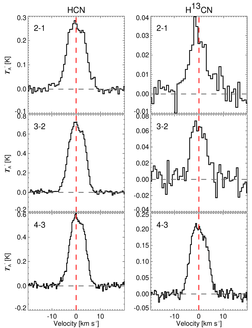
Figure 11: HCN emission in the survey: H¹²CN (left) and H¹³CN (right).

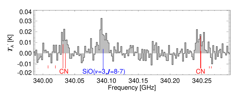
Figure 12: CN($3-2$) emission. The positions of the red vertical lines indicate the rest frequencies of the hfs components, and their lengths are proportional to the relative component strengths in LTE.

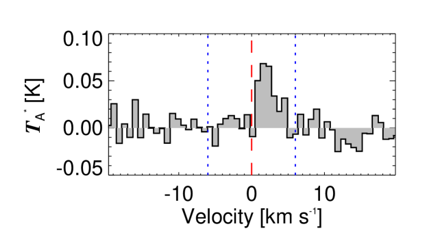
Figure 13: SO₂, $v_{2}=1$ ($J_{K_{a},K_{c}}=69_{9,61}-70_{6,64})$ emission.

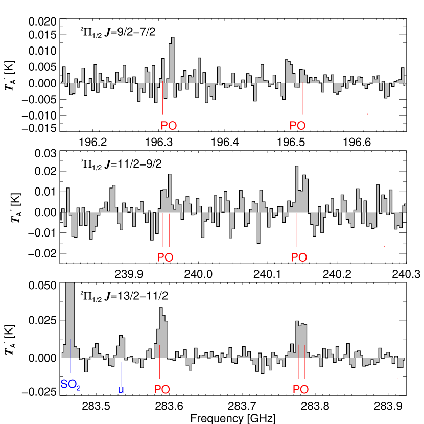
Figure 14: PO line emission. Vertical red lines mark the rest frequencies of the different hfs components of each rotational transition.

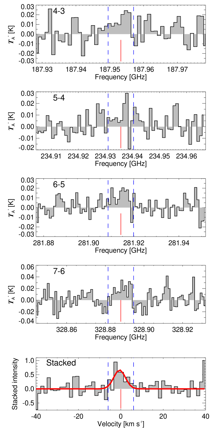
Figure 15: PN line emission. The first four panels show the spectra of the $J=4-3,\dots,7-6$ transitions; the bottom panel shows the peak-normalised result of stacking these at a velocity resolution of 1.5 km s^-1, weighted with the upper level statistical weights, $2J+1$ of the respective transitions. Red lines indicate the rest frequency (or $\varv=0$ km s^-1 in the bottom panel) of each transition, blue lines indicate velocities $\pm 6$ km s^-1 with respect to the stellar $\varv_{\mathrm{LSR}}$. The red curve in the bottom panel represents a Gaussian fit to the stacked data.

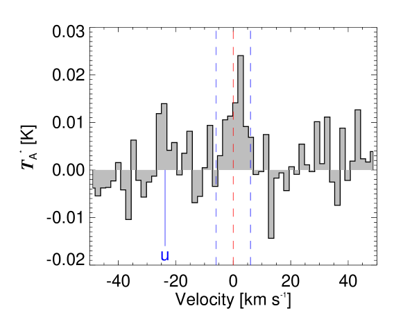
Figure 16: Tentative identification of PNO line emission. The red dashed line corresponds to the rest frequency of the PNO($J=25-24$) transition and the blue dashed lines indicate the stellar $\varv_{\mathrm{LSR}}$ $\pm 6$ km s^-1. In blue we indicate an unidentified emission feature.

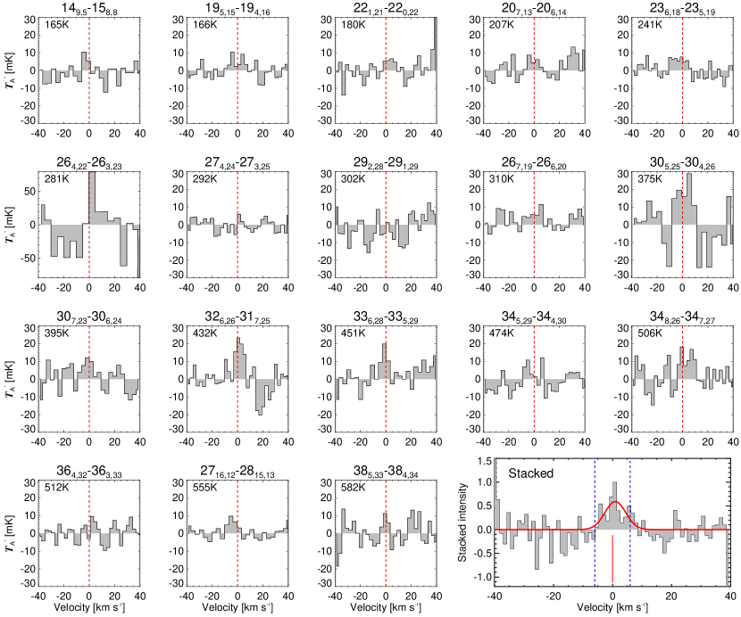
Figure 17: Tentative identification of TiO₂ line emission. Quantum numbers for each transition and upper-level energies $E_{\mathrm{up}}/k$ are given for each panel. The last panel shows the spectrum that results from stacking (in velocity space, at 1.2 km s^-1 resolution) the spectra in the other 18 panels, assuming equal weights. The red line represents a best-fit Gaussian curve to the stacked spectrum.

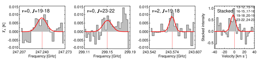
Figure 18: Tentative detection of NaCl line emission. The first three panels show tentative detections; for the $v=2,J=19-18$ spectrum, this is the combination of observations obtained at two different epochs (see text). The last panel shows a stacked spectrum using all rotational transitions (in $v=0$) marked in the top right-hand corner.

3.2.4 Hydrogen cyanide, cyanide

We detect emission from the $J=2-1,3-2$, and $4-3$ transitions of both H¹²CN and H¹³CN; see Fig. 11. Our observation of the H¹²CN($3-2$) line is consistent within 10% with the spectrum presented by Schöier et al. (2013). For the H¹²CN($4-3$) line the latter authors only listed an integrated intensity and did not show the spectrum. The integrated intensity in our survey is 77% of that reported by Schöier et al. (2013). This is within reasonable calibration uncertainties. We are not aware of earlier observations of the $J=2-1$ line or of any previously reported detections of H¹³CN for R Dor. We do not include radiative transfer modelling of H¹²CN and H¹³CN in this paper.

We do not detect CN($2-1$) emission, but we do detect two clear components of the CN($3-2$) line; see Fig. 12. These components coincide with the intrinsically brightest hyperfine structure components of the transition. We do not detect ¹³CN, in line with the intensity of the ¹²CN emission and the ¹²C/¹³C isotopic ratio derived by Ramstedt & Olofsson (2014).

3.2.5 Sulphur-bearing species

We identify 16 lines of ³²SO and 12 of ³⁴SO. We identify 118 lines of ³²SO₂ in the vibrational ground state, and 1 in the $v_{2}=1$ state (Fig. 13), 5 lines of ³⁴SO₂, 10 lines of SO¹⁸O, and 2 lines of SO¹⁷O.

Danilovich et al. (2016) presented detailed radiative transfer models of both the SO and SO₂ emission we observe towards R Dor, as well as towards several other oxygen-rich AGB stars. At the time of that publication, the survey had not been completed, and we have in the mean time identified more SO and SO₂ lines than were available then. A careful check between the lines observed in the range $159-211$ GHz and the model predictions shows an excellent agreement for 17 SO₂ and 3 SO lines, and an overprediction of the SO₂ lines $5_{2,4}-5_{1,5}$ at 165.1 GHz and $3_{2,2}-2_{1,1}$ at 208.7 GHz by about a factor of 2. We note here that the SO₂($12_{4,8}-12_{3,9}$) transition at 355.05 GHz modelled by Danilovich et al. (2016) has a peak-$T_{\mathrm{A}}^{*}$ of $\sim$0.05 K, whereas in additional data obtained in June 2016, it is 0.07 K. This indicates possible time variability in the excitation of SO₂, as is also mentioned by Danilovich et al. (2016).

We detect emission from SiS and CS only tentatively, consistent with the idea that SO and SO₂ are the main sinks of sulphur in low-mass-loss-rate M-type AGB stars (Danilovich et al. 2016). We refer to the latter study for details on the modelled abundance distributions and the implications for the chemical networks.

3.2.6 Phosphorus-bearing molecules

We detect multiple transitions of PO and PN, making R Dor the second oxygen-rich AGB star, after IK Tau (De Beck et al. 2013; Velilla Prieto et al. 2017), for which these species are detected.

Our observations cover three transitions of PO in the $\Omega=1/2$ lower-spin component: ${}^{2}\Pi_{1/2}\,J=9/2-7/2$, ${}^{2}\Pi_{1/2}\,J=11/2-9/2$, and ${}^{2}\Pi_{1/2}\,J=13/2-11/2$; see Fig. 14. The tentative detection of the first two is strengthened by the definite detection of the third transition. We detect none of the higher-energy $\Omega=3/2$ upper spin component transitions. Even though the strengths of the doublets in each transition reflect excitation in, or close to, LTE, the derivation of reliable values of excitation temperature and column density through a rotational-diagram analysis is hindered by the limited sensitivity reached in the observations and the lack of spatial information.

The survey covers four transitions of PN: $J=4-3,\dots,7-6$. We show spectra for all four in Fig. 15 and show the result of stacking these using the statistical weights of the upper levels, $2J+1$, as the weights for the transitions $J-J^{\prime}$. The resulting spectrum, stacked in velocity space at a velocity resolution of 1.5 km s^-1, shows emission at peak-$S/N=3.6$. We could not identify any other species that would contribute to the velocity range $[-10;10]$ km s^-1 in this stacked spectrum. The best-fit Gaussian profile to the stacked spectrum has a full width at half maximum of 6.8 km s^-1, comparable to what we see for high-$S/N$ line emission in the survey. We hence claim the presence of PN in the CSE of R Dor.

Although the peak flux densities for PO and PN for R Dor are higher than those for IK Tau for similar transitions by factors of a few, the sensitivity of our survey is unfortunately not sufficient to compare these detections of PO and PN directly to the results obtained for IK Tau by De Beck et al. (2013) and Velilla Prieto et al. (2017) using the SMA and the IRAM 30 m telescope. Dedicated single-tuning observations at high sensitivity are needed to further investigate the phosphorus-bearing molecules in R Dor.

We do not conclusively detect any other P-bearing molecules in our survey, but point out a tentative, and, if true, also first, detection of PNO. At 309.4 GHz we detect an emission feature that coincides with the rest frequency of PNO($J=25-24$); see Fig. 16. We can rule out image band contamination and spectrometer issues, leading to the conclusion that this is an actual emission feature. However, we cannot confirm a detection for any of the other transitions of PNO covered by the survey ($J=13-12,\dots,29-28$) and cannot find a stacked spectrum with a significant S/N. Therefore, this tentative detection should be regarded with caution.

We do not detect the ground-state PH₃($J_{K}=1_{0}-0_{0}$) line at 266.9 GHz. Based on the NH₃ brightness reported by Justtanont et al. (2012) and a P/N abundance ratio of $\sim$0.004 (Asplund et al. 2009), we estimate its peak intensity at $<2$ mK, whereas the sensitivity of our survey reaches 5.6 mK rms noise at a 2 km s^-1 resolution at this frequency. However, this is a zeroth-order estimate which assumes similar behaviour of NH₃ and PH₃, and an analogous estimate for IK Tau leads to a peak antenna temperature of $\sim$30 mK for the IRAM 30 m telescope, which is invalidated by the observations presented by Velilla Prieto et al. (2017).

We have successfully applied for ALMA Cycle 5 observations to observe PO, PN, and PH₃ in the CSEs of R Dor and IK Tau, but at the date of submission of this manuscript, no data have been obtained yet.

Table 3: Isotopic ratios retrieved from line-intensity ratios, with $R_{\mathrm{c}}$ the frequency-corrected ratio: per transition this corresponds to $R_{\mathrm{c}}=R_{\mathrm{a/b},J-J^{\prime}}$ and overall to $R_{\mathrm{c}}=R_{\mathrm{a/b}}$, the error-weighted mean ratio. When available, we also list the isotopologue abundance ratios $R_{\mathrm{RT}}$ obtained from radiative transfer modelling. Solar (elemental) isotopic ratios $R_{\odot}$ are taken from Asplund et al. (2009, see their Table 3). See text for details.

	Isotopologues	Transition	$R_{\mathrm{c}}$	$R_{\mathrm{RT}}$	$R_{\odot}$	Remarks
C	12CO/13CO	$2-1$	$17.0\pm 3.6$
		$3-2$	$9.1\pm 1.9$
			$10.9\pm 1.7$	10		$R_{\mathrm{RT}}$ from Ramstedt & Olofsson (2014).
	H12CN/H13CN	$2-1$	$8.4\pm 1.8$
		$3-2$	$9.0\pm 1.9$
		$4-3$	$2.4\pm 0.5$			H13CN($J=4-3$) is blended.
			$8.7\pm 1.3$			Excluding the $4-3$ transitions.
					12C/13C = 89.40
Si	28SiO/29SiO	$4-3$	$2.3\pm 0.5$
		$5-4$	$3.2\pm 0.7$
		$6-5$	$3.2\pm 0.7$
		$7-6$	$2.5\pm 0.5$
		$8-7$	$3.1\pm 0.7$
			$2.8\pm 0.3$	$12.6_{3.98}^{39.8}$	28Si/29Si = 19.69
	28SiO/30SiO	$4-3$	$4.0\pm 0.8$
		$5-4$	$4.3\pm 0.9$
		$6-5$	$4.2\pm 0.9$
		$7-6$	$4.1\pm 0.9$
		$8-7$	$4.0\pm 0.8$
			$4.1\pm 0.4$	$20.0_{6.31}^{63.1}$	28Si/30Si = 29.87
	29SiO/30SiO	$4-3$	$1.7\pm 0.4$
		$5-4$	$1.4\pm 0.3$
		$6-5$	$1.3\pm 0.3$
		$7-6$	$1.6\pm 0.3$
		$8-7$	$1.3\pm 0.3$
			$1.4\pm 0.1$	$1.58_{1.00}^{2.51}$	29Si/30Si = 1.517
O	28Si16O/28Si17O	$4-3$	$76.3\pm 16.2$
		$5-4$	$65.7\pm 13.9$
		$6-5$	$54.0\pm 11.5$
		$7-6$	$57.1\pm 12.1$
		$8-7$	$61.6\pm 13.1$
			$61.2\pm 5.8$	$398_{200}^{2000}$	16O/17O = 2632
	28Si16O/28Si18O	$4-3$	$38.1\pm 8.1$
		$5-4$	$47.9\pm 10.1$
		$6-5$	$30.6\pm 6.5$
		$7-6$	$24.9\pm 5.3$
			$31.5\pm 3.4$	$251_{100}^{1000}$	16O/18O = 498.8
	28Si17O/28Si18O	$4-3$	$0.5\pm 0.1$
		$5-4$	$0.7\pm 0.2$
		$6-5$	$0.6\pm 0.1$
		$7-6$	$0.4\pm 0.1$
			$0.5\pm 0.1$	$0.631_{0.398}^{0.794}$	17O/18O = 0.190
	C16O/C17O	$2-1$	$-$
		$3-2$	$-$
			$-$	$>200$		Non-detection of C17O emission.
	C16O/C18O	$2-1$	$-$
		$3-2$	$-$
			$-$	$>200$		Non-detection of C18O emission.
S	32SO2/34SO2	Overall spectrum		$21.6\pm 8.5$	32S/34S = 22.1	$R_{\mathrm{RT}}$ from Danilovich et al. (2016)

3.2.7 Heavy metal species: titanium, aluminium, sodium

Titanium- and aluminium-bearing molecules could be critical in the dust-condensation process, and much effort has recently gone into searching for such species (De Beck et al. 2015b, 2017; Decin et al. 2017; Kamiński et al. 2013a, 2016, 2017).

We do not detect any emission from TiO in this survey, but claim a possible detection of TiO₂, based on a peak S/N of $\sim$3 in the stacked spectrum of a set of 18 low-$S/N$ tentative detections; see Fig. 17. The sensitivity of the observations is, however, not sufficient to set up a relevant abundance or rotational-diagram analysis. One emission feature in the spectrum agrees with a component of TiN ($8-7$), which, if confirmed, would be a first detection of this molecule in space. However, if true, we only detect one of the two doublet components of the $8-7$ transition at 297.4 GHz clearly, although their theoretical strengths are identical. Furthermore, we do not detect emission of any other TiN transition in this survey ($5-4,\dots,9-8$). Image sideband contamination is ruled out and we can identify no other candidate carrier for this feature. Additionally, investigation of the survey of IK Tau from Velilla Prieto et al. (2017) shows a low-level peak at the same position, 297.4 GHz, further supporting that this is a genuine spectral feature (Sect. 3.4).

We detect no emission from the aluminium-bearing species AlO, AlOH and AlCl with certainty, although 4, 6, and 14 transitions, respectively, are covered by the survey (AlO: $6-5,\dots,9-8$; AlOH: $6-5,\dots,11-10$; AlCl: $11-10,\dots,25-24$). In the case of AlO, only a tentative detection could possibly be claimed for the $9-8$ transition (De Beck et al. 2017). Stacking of these lines is difficult owing to the hyperfine structure of the individual transitions not lining up in velocity space. Recent ALMA observations at much higher sensitivity detect these species in the CSEs of R Dor and IK Tau (Decin et al. 2017), with peak flux densities consistent with the non-detections in our APEX observations.

We tentatively detect emission from NaCl in the vibrational ground state $v=0$ ($J=19-18,23-22$) and in the $v=2$ vibrationally excited state ($J=19-18$) at $S/N$ of about 3, 2.5, and 5, respectively; see Fig. 18. The part of the spectrum with the $v=2$ emission was observed at two different dates, one time in September 2011 and the other in November 2015. We see a change in both the intensity and width of the measured profile between the two observations. The aforementioned $S/N$ is for the combined spectrum. Given the likely radiative excitation of such vibrationally excited transitions, this line variability is possibly linked to stellar variability. Given the sensitivity of our survey data we cannot conclusively identify other lines of NaCl in the spectrum at an acceptable S/N. Figure 18 additionally shows a stacked spectrum combining all parts of the spectrum where NaCl (in the vibrational ground state $v=0$) has rotational transitions and that are not obviously contaminated by line emission from other species or by high noise. The resulting Gaussian fit has a $S/N\approx 3$, further supporting the tentative identification of NaCl emission in the spectrum. Multiple emission lines of NaCl, in the vibrational ground state as well as in vibrationally excited states, have been detected towards IK Tau and VY CMa (Milam et al. 2007; Decin et al. 2016; Velilla Prieto et al. 2017).

Table 4: Unidentified emission features.

Frequency	$T_{A\mathrm{,peak}}^{*}$	$FWHM$	$\delta\varv$	Remarks
(MHz)	(mK)	(km s-1)	(km s-1)
173514	56	7.4	1.1
189362	10	13.2	2.9
204008	9	8.2	2.7
225998	10	11.1	2.4
267993	16	5.1	2.0
273284	61	7.6	1.1
280051	14	5.0	1.6
283535	13	9.3	1.9
295629	25	9.0	1.9
297404	17	16.0	1.8	Also seen towards IK Tau. TiN only tentative candidate.
298464	16	7.5	1.8
309449	13	3.9	1.4
319253	10	8.0	1.8
320204	46	7.8	0.9
332217	42	6.3	0.9
354195	1600	–	0.5	Maser. H2SiO? See Sect. 3.4.1.

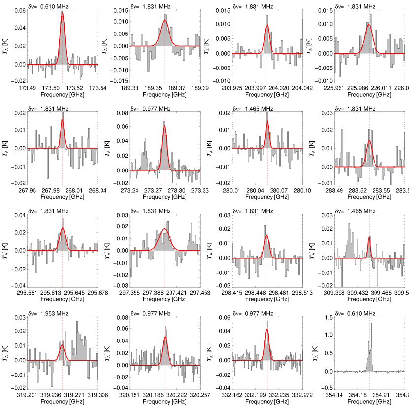
Figure 19: Unidentified line emission features. We fit a single Gaussian line profile to each of these, except the suspected maser line at 354 GHz, and list the retrieved central frequency, peak intensity, and FWHM at the given velocity resolution in Table 4. The corresponding frequency resolution $\delta\nu$ of the spectra is given at the top left of each panel.

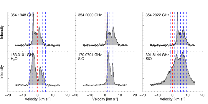
Figure 20: Alignment in velocity space of unidentified emission at $\sim$354.2 GHz (top) with known maser emission (bottom). The spectra shown in the top panels, from left to right, assume rest frequencies of 354.1948 GHz, 354.2000 GHz, and 354.2022 GHz, respectively. The bottom panels show, from left to right, H₂O ($J_{K_{\rm a},K_{\rm c}}=3_{1,3}-2_{2,0}$) at 183.3 GHz, SiO ($v=3,J=4-3$) at 170.1 GHz, and SiO ($v=1,J=7-6$) at 301.8 GHz. Vertical dashed lines indicate emission components similar to those mentioned in the discussion in Sect. 3.

3.3 Isotopes

Our survey covers emission from isotopologues containing different isotopes of carbon (¹²C, ¹³C), oxygen (¹⁶O, ¹⁷O, and ¹⁸O), silicon (²⁸Si, ²⁹Si, ³⁰Si), and sulphur (³²S, ³⁴S).

Accurate isotopic ratios of different elements carry information on the evolutionary stage and/or the initial mass of an AGB star, based on the assumption that the circumstellar (molecular) isotopologue ratios are representative of the atmospheric (elemental) isotopic ratios. This assumption is reasonable, since the only currently known chemical processes involved in changing the isotopologue ratio are fractionation in the very coldest parts of the CSE and isotope-selective photodissociation, for example, of CO (Visser et al. 2009). Saberi et al. (2017) discuss the difference between ¹²CO/¹³CO and H¹²CN/H¹³CN in the CSE of the AGB star R Scl as a result of isotope-selective photodissociation in the case of CO, and how, consequently, H¹²CN/H¹³CN is likely more representative of the stellar ¹²C/¹³C in certain cases. Since the dissociation of SiO is in the continuum, we expect our derived isotopologue ratios to be representative also for the elemental isotopic ratios of silicon and oxygen.

We summarise intensity ratios for a large set of isotopologue emission lines in our survey in Table 3. These transition-specific values, $R_{\mathrm{a/b},J-J^{\prime}}$, are obtained as

$$R_{\mathrm{a/b},J-J^{\prime}}=\frac{I_{\mathrm{a},J-J^{\prime}}}{I_{\mathrm{b},J-J^{\prime}}}\times\left(\frac{\nu_{\mathrm{a},J-J^{\prime}}}{\nu_{\mathrm{b},J-J^{\prime}}}\right)^{-3},$$ (3)

where $\nu_{J-J^{\prime}}$ is the rest frequency of each rotational transition $J-J^{\prime}$, $I_{J-J^{\prime}}$ is its integrated line intensity, and ‘a’ and ‘b’ denote the different isotopic variations. The cubic frequency-dependent correction factor accounts for the difference in beam-filling (when all lines are assumed spatially unresolved) and in intrinsic line strength (see e.g. Schöier & Olofsson 2000; De Beck et al. 2010). We also list approximate isotopologue ratios $R_{\mathrm{a/b}}$, calculated as the weighted average of the transition-specific values, assuming the uncertainties as the inverse weights. We note that these ratios are sometimes obtained from optically thick line emission, which is likely when a highly abundant isotopologue is considered and is very clear in the case of ²⁸SiO, so in these cases the obtained ratio should be considered a limiting value. Only the isotopologue ratios obtained from detailed radiative transfer modelling ($R_{\mathrm{RT}}$) and those derived from exclusively optically thin line emission are representative of the actual isotopic ratio in the CSE. All calculations of line ratios in this section are based on a 15% uncertainty on the line intensities. This is reasonable, and maybe rather conservative, given that most lines that are compared directly have been observed (quasi-)simultaneously and are almost always observed with the same instrument.

3.3.1 Carbon: CO, HCN

Ramstedt & Olofsson (2014) determine ¹²CO/¹³CO to be $\sim$10 for R Dor, based on radiative transfer modelling of CO. Although optical depth could affect the line ratios for both CO and HCN, the values we find from line intensity ratios are consistent with the value derived by Ramstedt & Olofsson (2014). We do not re-model the CO line emission, nor model the HCN line emission here, but plan a detailed radiative transfer analysis of the H¹²CN and H¹³CN line emission in the future.

The derived ¹²C/¹³C is significantly lower than any values predicted by theoretical models, an issue also discussed by Ramstedt & Olofsson (2014).

3.3.2 Oxygen: SiO

From the line intensity ratios we find an isotopologue abundance ratio ²⁸Si¹⁷O/²⁸Si¹⁸O$\approx 0.5\pm 0.1$ (Table 3). From the radiative transfer modelling presented in Sect. 3.2.2, we derive ²⁸Si¹⁷O/²⁸Si¹⁸O=$0.6\pm 0.2$. Assuming that the isotopologue abundance ratio derived for the CSE is equal to the elemental ¹⁷O/¹⁸O isotopic ratio at the stellar surface we find that ¹⁷O/¹⁸O$=0.6\pm 0.2$, implying an initial mass, $M_{\rm i}$ for R Dor of $1.4_{-0.1}^{+0.2}$ $M_{\sun}$ (Karakas & Lugaro 2016; Cristallo et al. 2015, assuming solar metallicity).

Independently from the study presented here, Danilovich et al. (2017a) model the emission of several transitions of H${}_{2}^{17}$O and H${}_{2}^{18}$O towards R Dor and derive isotopologue abundance ratios o-H${}_{2}^{17}$O/o-H${}_{2}^{18}$O=$0.54\pm 0.26$ and p-H${}_{2}^{17}$O/p-H${}_{2}^{18}$O=$0.30\pm 0.10$ for ortho-H₂O and para-H₂O, respectively, from which they derive an initial mass in the range $1.0-1.3$ $M_{\sun}$, although a slightly larger range of $1.0-1.6$ $M_{\sun}$ seems to better reflect their results. These results are in agreement with our findings based on the SiO emission, increasing the reliability of the derived ¹⁷O/¹⁸O for the CSE and of the inital mass estimate, under the assumptions made.

We do not detect C¹⁷O or C¹⁸O in our survey. Assuming the abundance ratios Si¹⁶O/Si¹⁷O and Si¹⁶O/Si¹⁸O to be representative of C¹⁶O/C¹⁷O and C¹⁶O/C¹⁸O, we run radiative transfer models for C¹⁷O and C¹⁸O. The predictions for the $J=2-1$ and $J=3-2$ transitions are in agreement with formal non-detections in the survey, with peak intensities well below 10 mK and 20 mK for the respective transitions, for both C¹⁷O and C¹⁸O for peak abundances $f_{0}<10^{-6}$. Such high values of $f_{0}$ were considered only because of the large uncertainties on the SiO isotopologue abundance ratios. This upper limit to the abundances means that the uncertainty on ¹⁸O/¹⁶O is smaller than given by our radiative-transfer modelling results in Table 3, and can be constrained to a lower limit of 200.

Based on the evolutionary models of Karakas & Lugaro (2016) and Cristallo et al. (2015), our estimate of $M_{\rm i}=1.3-1.6$ $M_{\sun}$ implies that if R Dor becomes a carbon-rich AGB star it will only do so in its final phases with a C/O ratio only slightly above 1. During its lifetime of $\sim 1.6$ Myr on the thermally pulsing AGB (TP-AGB), the star would dredge up $\lesssim 0.01$ $M_{\sun}$. According to Karakas & Lugaro (2016), this would happen over the course of $\sim$16 TP cycles, whereas Cristallo et al. (2015) quote only 5 TP cycles for a star with $M_{\rm i}=1.5$ $M_{\sun}$.

3.3.3 Silicon: SiO

From the radiative transfer modelling described in Sect. 3.2.2 we derive isotopologue abundance ratios ${}^{28}\mathrm{SiO}/^{29}\mathrm{SiO}=12.6^{79.4}_{1.6}$, ²⁸SiO/³⁰SiO=$20.0^{79.4}_{2.0}$, and ${}^{29}\mathrm{SiO}/^{30}\mathrm{SiO}=1.6_{0.4}^{6.3}$. The latter is in good agreement with the line intensity ratio $R_{{}^{29}\mathrm{SiO}/^{30}\mathrm{SiO}}=1.4\pm 0.1$ (Table 3). These derived ratios are in agreement with the solar isotopic ratios ²⁹Si/³⁰Si=1.5 and ²⁸Si/³⁰Si=29.9 (Asplund et al. 2009). The models of Karakas & Lugaro (2016) indeed show no, or insignificant, changes in ²⁸Si/²⁹Si and ²⁸Si/³⁰Si as a consequence of AGB evolution for initial masses $\leq 2$ $M_{\sun}$.

3.3.4 Sulphur: SO, SO₂

Danilovich et al. (2016) derived ³²S/³⁴S$=22\pm 9$ from detailed radiative transfer models of SO and SO₂. This is in good agreement with the solar value ³²S/³⁴S=22.1 (Asplund et al. 2009) and the model results that sulphur does not show significant changes in its isotopic ratios throughout AGB evolution.

3.3.5 Evolutionary stage

In order to constrain not only the initial mass of R Dor, but also its evolutionary stage, we need observationally determined isotopic ratios for, for example, nitrogen (¹⁴N/¹⁵N) and aluminium (²⁶Al/²⁷Al), based on highly sensitive observations. Furthermore, there is a strong need for better constrained theoretical models for the variation of ¹²C/¹³C throughout the AGB evolution. We refer to Ramstedt & Olofsson (2014) for an in-depth discussion on the low ¹²C/¹³C found for oxygen-rich AGB stars compared to stellar evolution models.

3.4 Unidentified lines

We list the unidentified features in Table 4 with the rest frequencies, peak intensities, and $FWHM$:s obtained from a Gaussian line profile fitting and show the spectra and their fits in Fig. 19. The listed velocity resolution gives a $S/N\geq 3$ for the Gaussian fit in all cases. For all unidentified features we are able to rule out instrumental effects and image contamination, thanks to the coverage of our survey. None of these lines are reported for the SMA and IRAM 30 m surveys of IK Tau, VY CMa, or IRC +10 216 (De Beck et al. 2013; Kamiński et al. 2013b; Patel et al. 2011; Velilla Prieto et al. 2017). One unidentified feature, at 297.4 GHz, seems to be present in the IRAM 30 m survey of IK Tau, but was not explicitly reported by Velilla Prieto et al. (2017). The fully independent detections of this feature towards two significantly different CSEs and using two different telescopes suggests that it is genuine.

3.4.1 A new maser at 354.2 GHz

The most striking unidentified feature appears at 354.2 GHz and is markedly maser-like in its shape. The emission reaches a peak antenna temperature of $\sim$1.6 K ($\sim$66 Jy; peak-$S/N\approx 55$ at 0.1 km s^-1 resolution), and a total integrated intensity of 4.7 K km s^-1 ($\sim$193 Jy km s^-1). A detailed check of the collected data reveals that this feature is present in all consecutively obtained individual scans and that its distinct shape is repeated in all of these. In combination with the resemblance to other spectral lines in the survey (see discussion below) this leads us to believe that this feature is a real spectral emission line.

We compare the emission feature to three maser lines in our survey with a similar shape, H₂O($J=3_{1,2}-2_{2,0}$) at 183.3 GHz, SiO($v=3,J=4-3$) at 170.1 GHz, and SiO($v=1,J=7-6$) at 301.8 GHz, in Fig. 20. In order to align the peaks in the unidentified feature with those of the former two, we need to centre the line at 354.195 GHz and 354.200 GHz, respectively. This shift is due to the fact that the H₂O line emission originates in both the blue and red sides of the wind, whereas this particular SiO maser seems to originate almost exclusively from the redshifted part of the wind. From the comparison in Fig. 20, it seems that the emission could be ”H₂O-like”, rather than ”SiO-like” when one considers that the reddest emission in the profile has no counterpart in the SiO maser emission. However, the closest known H₂O maser to this frequency lies at 354.8 GHz (Gray et al. 2016) and none of the listed transitions of the isotopologues H${}_{2}^{17}$O and H${}_{2}^{18}$O coincide with this frequency, either.

Searching the spectroscopic catalogues we found only the ortho-H₂SiO (silanone) doublet $J_{K_{\mathrm{a}},K_{\mathrm{c}}}=10_{4,7}-9_{4,6}$ and $J_{K_{\mathrm{a}},K_{\mathrm{a}}}=10_{4,6}-9_{4,5}$ to be a potential candidate. The doublet is located at 354202.1540 MHz, with lower and upper level energies of 191 K and 208 K, respectively. The upper limit on the uncertainty on this rest frequency listed in CDMS is 0.02 MHz. If confirmed, this is, to our knowledge, the first detection of this molecule in space. Assuming this as the rest frequency moves the emission entirely to the red velocities, with little or no resemblance with the H₂O maser and the first SiO maser in Fig. 20. However, the maser emission of the SiO($v=1,J=7-6$) line at 301.8 GHz (rightmost bottom panel in Fig. 20) is also dominated by red-shifted emission and shows some distinct peaks that might very well correspond to those seen in the new feature. Recently, Gobrecht et al. (2016) predicted that H₂SiO can reach abundances of up to $10^{-6}-10^{-5}$ in the inner wind of the oxygen-rich, high-mass-loss-rate Mira-type variable IK Tau. H₂SiO, together with HSiO, is thought crucial in the nucleation of silicate dust clusters. Whether or not these predictions can be used as representative of the low-mass-loss-rate, semi-regular variable R Dor is not clear. We do not detect any other emission from H₂SiO in our survey, even though transitions over a large range of excitation energies are covered. Given the maser nature of the emission line tentatively identified as H₂SiO, it is difficult to assess whether the non-detections are consistent with this detection.

Additional observations at this frequency, carried out on 9 June 2016, unfortunately do not reveal any trace of the emission at a $\sim$10 mK rms noise level at 2 km s^-1 resolution. Archival observations of R Dor, obtained with APEX on 26 March 2008, equally show no detectable emission at 354.2 GHz, however at a much worse rms noise of $\sim$400 mK. We point out that the survey observations at this particular frequency were carried out on 1 September 2011, when the light curve variations of R Dor were quite regular. Currently, however, R Dor’s light curve is much more chaotic and shows smaller overall amplitude changes (source: AAVSO). Considering the maser nature of the line, this change might very well significantly affect the excitation of this unidentified line.

Observations at this frequency and other frequencies of likely observable line emission in the H₂SiO spectrum should also be obtained for a larger sample of AGB stars, with an initial focus on M-type stars in order to understand the physical conditions under which this maser line could be excited.

4 Comparison to other line surveys

Spectral surveys of CSEs of M-type evolved stars have been published only in recent years. This includes the AGB stars IK Tau and OH 231.8 +4.2 (De Beck et al. 2013, 2015a; Sánchez Contreras et al. 2011, 2015; Velilla Prieto et al. 2015, 2017), the red supergiant VY CMa Kamiński et al. (2013b), and the yellow hypergiant IRC +10420 (Quintana-Lacaci et al. 2016). All of these stars lose mass at high rates (roughly $\gtrsim 0.5\times 10^{-5}$ $M_{\sun}$ yr^-1; e.g. De Beck et al. 2010; Velilla Prieto et al. 2015, and references therein), leading to significantly higher densities in their CSEs than is the case for R Dor, with its low mass-loss rate and low expansion velocity ($\dot{M}=1-2\times 10^{-7}$ $M_{\sun}$ yr^-1, $v_{\rm exp}=5.7$ km s^-1; Maercker et al. 2016). Apart from IK Tau and R Dor, all of these sources have been shown to have outflows that very strongly deviate from smooth, spherical, constant winds (e.g. Bujarrabal et al. 2002; Castro-Carrizo et al. 2007; Richards et al. 2014, and references therein). Given all of the above, we only compare our results to those obtained for IK Tau.

Figure 25 shows a direct comparison of our APEX data of R Dor with the IRAM 30 m data of IK Tau from Velilla Prieto et al. (2017) scaled to account for the difference in intensity that would be an effect of the different mass-loss rate and distance of the two objects and for the difference in point-source sensitivity between the telescopes (see App. C). The sensitivity reached in the spectral scan of IK Tau is better than that of the R Dor spectral scan presented here. However, the ratio of the rms noise to the peak intensity of the closest CO emission lines is similar when assuming a spectral resolution (2 MHz and 0.6 MHz for IK Tau and R Dor, resp.) that results in the same number of spectral elements covering the full line width of twice the expansion velocity ($v_{\rm{exp}}$ is 18.5 km s^-1 and 5.7 km s^-1 for IK Tau and R Dor, resp.). This allows us, to a certain degree, to compare the two surveys.

Both surveys show many spectral features pertaining to SO₂ and SiO, including isotopologues and multiple vibrational states, with strong emission lines from SiS and CS notably missing from the R Dor spectrum. The observations of IK Tau reveal several other molecules that we do not detect towards R Dor: H₂S, NS, HNC, NO, H₂CO, and HCO⁺. We do not detect any molecules towards R Dor that are not seen towards IK Tau, apart from (tentatively) some specific, low-abundance isotopologues. At the same time, it is remarkable that none of the R Dor u-lines (except for possibly one) are seen in the IK Tau spectrum.

Danilovich et al. (2016) already reported that SO and SO₂ are the main reservoirs of S in the CSE of R Dor and that their abundances roughly decrease with increasing mass-loss rate when also studying other M-type CSEs (including IK Tau). Danilovich et al. (2017b) reported that H₂S is unlikely to play any significant role at mass-loss rates $\lesssim 5\times 10^{-6}$ $M_{\sun}$ yr^-1. This is consistent with the lack of CS, SiS, and H₂S in R Dor.

Assuming the simple scale factor quoted above, we find that all HNC, NO, H₂CO, or HCO⁺ emission lines would fall below the detection limit of our observations. Additionally, assuming that the HNC/HCN intensity ratios found for IK Tau also hold for R Dor, further supports the non-detection of all observed HNC transitions ($J=2-1,3-2,4-3$). Considering this, we cannot rule out that R Dor would show emission from these molecules in more sensitive observations and cannot claim, from our survey results, a difference in chemistry to be at the base of the absence of emission from these in the case of R Dor. However, this difference is clearly at the base of the differences seen between the sulphur-bearing species in the two CSEs. Stacking did not lead to tentative detections for any of these molecules.

The H₂O isotopologue model results of Danilovich et al. (2017a) imply $M_{\rm i}=1.0-1.6$ $M_{\sun}$ for both R Dor and IK Tau. The integrated line intensities of Si¹⁷O and Si¹⁸O reported by Velilla Prieto et al. (2017), unfortunately, do not constrain very well the ratio Si¹⁷O/Si¹⁸O, making an independent estimate of ¹⁷O/¹⁸O impossible. The fact that the two stars appear so different in terms of pulsational and mass-loss properties (IK Tau is a Mira, R Dor is an SRb variable; their mass-loss rates differ by $1-2$ orders of magnitude) leads us to hypothesise that IK Tau could be in a later stage of its AGB evolution than R Dor, considering the trend of increasing mass-loss rate, expansion velocity, luminosity, and pulsation period with evolution along the TP-AGB (e.g. Vassiliadis & Wood 1993).

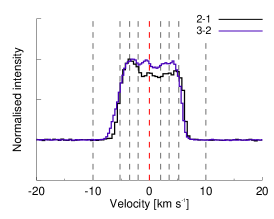
(a) CO

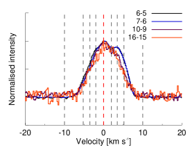
(b) CO, HIFI

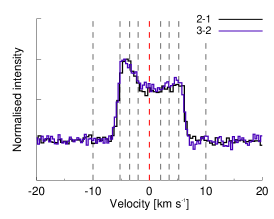
(c) ¹³CO

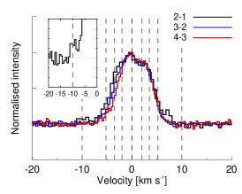
(d) HCN

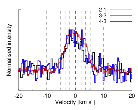
(e) H¹³CN

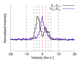
(f) H₂O

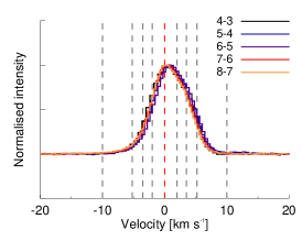
(g) ²⁸SiO

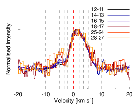
(h) ²⁸SiO, HIFI

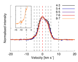
(i) ²⁹SiO

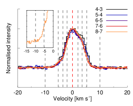
(j) ³⁰SiO

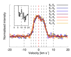
(k) SO (selection)

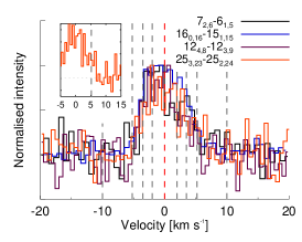
(l) SO₂ (selection)

Figure 21: Line shapes. Vertical dashed lines correspond to velocities $0$ km s^-1, $\pm 2.0$ km s^-1, $\pm 3.5$ km s^-1, and $\pm 5.2$ km s^-1 with respect to the stellar $\varv_{\mathrm{LSR}}$, where distinct emission features appear in multiple of the presented lines. Insets (with the same colour coding as the main plots) are added to several of the panels for increased visibility of these substructures.

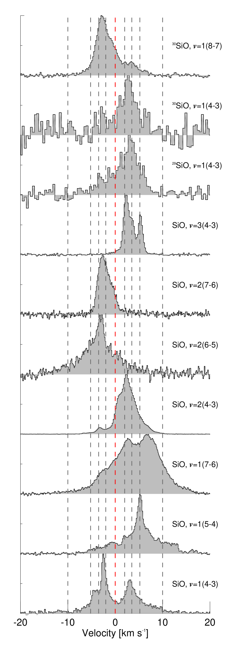
Figure 22: Selected SiO maser emission lines. Vertical dashed lines correspond to the velocities (relative to the stellar $\varv_{\mathrm{LSR}}$) 0.0 km s^-1, $\pm 2.0$ km s^-1, $\pm 3.5$ km s^-1, $\pm 5.2$ km s^-1, and $\pm 10.0$ km s^-1. Intensities are normalised to the peak and vertical offsets are added for visibility. We note that the observations are not coeval; see App. B.

5 Outflow kinematics

In case of a smooth, spherical wind described by a constant mass-loss rate, one expects a smooth line profile in the range flat-topped to parabolic for spatially unresolved emission, while spatially resolved emission leads to enhanced (in a relative sense) emission at the extreme velocities, where the lines may even become double-horned. The line profiles in the survey are largely represented by this range of profiles, indicating that the outflow of R Dor can, most likely, be approximated by a spherical wind. However, we do find multiple peaks in several line profiles, indicative of deviations from this simple structure. The CO emission lines observed with APEX and HIFI (Justtanont et al. 2012) show a small bump at the stellar $\varv_{\mathrm{LSR}}$ and several features at other velocities. In Fig. 21 we show the presence of a distinct emission feature in several lines, pertaining to different species, at $-5.2$ km s^-1 with respect to the systemic velocity. This is clearest for the SiO lines, in particular for ²⁹SiO and ³⁰SiO ($J=4-3,\dots,8-7$; Figs. 21(i) and 21(j)), and for ²⁸SiO observed with HIFI ($J=12-11,\dots,28-27$; Fig. 21(h)). An analogous red-shifted component at $5.2$ km s^-1 is marginally visible in the HIFI observations of CO ($J=10-9$ and $16-15$; Fig. 21(b)) and is more clearly seen in the emission of, for example, SO₂ ($7_{2,6-6_{1},5},16_{0,16}-15_{1,15},12_{4,8}-12_{3,9},25_{3,23}-25_{2,24}$; Fig. 21(l)). These lines have $E_{\mathrm{up}}/k$ of 36, 121, 111, and 326 K, tracing a large range of excitation energies. Based on the above, the features at $\mbox{$\varv_{\mathrm{LSR}}$}\pm 5.2$ km s^-1 are probably real. We additionally propose the existence of features at $\pm 2.0$ km s^-1 and $\pm 3.5$ km s^-1 with respect to the stellar $\varv_{\mathrm{LSR}}$. We show a selection of SiO maser emission lines in Fig. 22 and indicate the $\pm 2.0$, $\pm 3.5$ km s^-1 and $\pm 5.2$ km s^-1 positions. These velocities in many cases correspond to individual maser peaks, or have peaks that fall exactly in between them, strengthening the idea that these velocities are linked to some physical structure in the outflow.

Furthermore, the o-H₂O($1_{1,0}-1_{0,1}$) line observed with HIFI and shown by Maercker et al. (2016) shows clear bumps in the profile on both the red- and blue-shifted sides of the main emission component, at about $\pm 10$ km s^-1. We see similar bumps for different lines in our survey, for example HCN($2-1$) and SO($6_{5}-5_{4}$), albeit at a low intensity level. At $\pm 10$ km s^-1 we also detect maser emission in, for example, SiO($v=1,J=5-4,7-6$) and SiO($v=2,J=6-5$); see Fig. 22.

We conclude that the spectrally resolved emission lines of R Dor show signs of tracing up to five components in the CSE of R Dor: (1) a dominant component centred at the stellar $\varv_{\mathrm{LSR}}$ (6.5 km s^-1), and components that arise at (2) $\pm$2.0 km s^-1, (3) $\pm 3.5$ km s^-1, (4) $\pm 5.2$ km s^-1, and (5) $\pm\sim 10$ km s^-1 with respect to the stellar $\varv_{\mathrm{LSR}}$. From our spatially unresolved observations, we cannot readily draw conclusions on the geometry of these extra components. Their apparent symmetry around the $\varv_{\mathrm{LSR}}$ likely excludes that they are “random” inhomogeneities in the outflow and might imply that they are spatially confined in, for example, rings, shells, or spiral arms, but this is not an entirely straightforward explanation. The components are traced by line emissions of various molecular species that do not necessarily reside in the same parts of the CSE, and by transitions with very different excitation properties. Also, since the main wind has an expansion velocity of 5.7 km s^-1 (e.g. Maercker et al. 2016) the extra emission at $\sim$10 km s^-1 poses a problem in a smooth, monotonously accelerating wind. We very carefully speculate that this could be a higher-velocity outflow component very close to the star, given that we see it in SiO maser line emission and H₂O line emission, both believed to originate close to the star. Observations that resolve the emission both spectrally and spatially are clearly necessary to constrain the kinematics and geometry of the outflow and its possible components.

6 Conclusions

We present a spectral scan of the circumstellar environment of the oxygen-rich AGB star R Dor over the range $159.0-368.5$ GHz, interrupted at $321.5-338.5$ GHz. We carried out the observations with the APEX telescope, using the new SEPIA/Band-5 and the SHeFI facility instruments. This is the first survey of the circumstellar emission from this nearby, low-mass-loss-rate star over a large frequency range and is only the second such survey published in its entirety for an oxygen-rich AGB star after the one for IK Tau by Velilla Prieto et al. (2017). Thus far, efforts have mainly been targeted at carbon-rich and high-mass-loss rate objects such as IRC +10 216 or red supergiants such as VY CMa.

The survey exhibits roughly 320 spectral features (omitting those linked to instrumental effects). The flux in the spectrum is heavily dominated by thermal and maser emission from the different SiO isotopologues. In numbers, the SO₂ emission lines dominate by far. We detect several lines of CO (¹²CO and ¹³CO), HCN (H¹²CN and H¹³CN), SiO (²⁸SiO, ²⁹SiO, ³⁰SiO, Si¹⁷O, Si¹⁸O), CN, H₂O, SO, and SO₂. We detect PO and PN, the latter through a stacked spectrum, for the first time towards this source, but cannot claim the conclusive detection of any other P-bearing molecules. We note that ALMA observations will be performed to study in more detail the phosphorous chemistry in the CSEs of R Dor and IK Tau. We suggest the tentative detection of TiO₂, also from a stacked spectrum, AlO, and NaCl in the spectrum. These species are considered potentially important in the dust-condensation process. Sixteen features are currently still unidentified. Of these, one is a very strong maser at 354.2 GHz, which is possibly identifiable as H₂SiO (silanone). We could not confirm the presence of this emission in R Dor’s spectrum at a later time, but are positive that we are dealing with a real spectral feature and not an instrumental effect of any type.

We present radiative transfer models for the thermal emission in the vibrational ground state ($v=0$) of five silicon monoxide isotopologues: ²⁸SiO, ²⁹SiO, ³⁰SiO, Si¹⁷O, and Si¹⁸O. Radiative transfer models of the SO and SO₂ emission in a large part of the survey was already presented by Danilovich et al. (2016).

We provide estimates for isotopic ratios for C, O, Si, and S, both from line-intensity ratios and from radiative transfer models. Using the derived circumstellar Si¹⁷O/Si¹⁸O as a proxy for the stellar ¹⁷O/¹⁸O we constrain the initial mass of R Dor to the range $1.3-1.6$ $M_{\sun}$.

We find detailed features in the emission line profiles that arise in many of the emission lines, both thermal and maser emission, spread throughout the full spectrum and also in several emission lines measured with Herschel/HIFI. We suggest that these could trace up to five components in the CSE of R Dor: (1) a dominant smooth component centred at the stellar $\varv_{\mathrm{LSR}}$, and components that arise at (2) $\pm 2.0$ km s^-1, (3) $\pm 3.5$ km s^-1, (4) $\pm 5.2$ km s^-1, and (5) $\pm\sim 10$ km s^-1 with respect to the stellar $\varv_{\mathrm{LSR}}$. The presence of these indicates possible deviations in the wind of R Dor from a smooth, spherical outflow. Spatially and spectrally resolved observations are needed to decipher what these components could be.

Appendix A CO monitoring

We show observations of CO emission with single-dish facilities in Fig. 23. The CO($J=1-0,2-1,3-2$) emission was observed $1990-2000$ using the Swedish-ESO Submillimetre Telescope (SEST). The CO($J=2-1,3-2,4-3$) emission was repeatedly observed with APEX in the time frame $2005-2014$. The spectra at different epochs can be used to investigate possible variability in the CO emission of R Dor. Unfortunately, we do not have any recent observations of the $J=1-0$ line, whereas we mainly have recent observations for the higher-$J$ lines, and only a few or none from the 1990s, complicating a coherent time-variability study of the CO emission.

The $J=1-0$ spectra from the two earliest epochs (1991, 1992) agree very well. The third epoch (1993) shows the presence of an emission feature at $2-5$ km s^-1 red-shifted with respect to the systemic velocity, which is not seen in the earlier epochs. This ”extra” peak matches quite well in velocity the features seen in, for example, the CO emission in our APEX survey data (Figs. 21(a) and 3) or in any of the $J=2-1,3-2,4-3$ spectra shown in Fig. 23. We do not have a straightforward explanation for this change in the emission feature of the $J=1-0$ line. We remind the reader that the $e$-folding radius for the CO abundance distribution is about $1.6\times 10^{16}$ cm (36″in diameter; Maercker et al. 2016) and that the emitting region of this transition covers a large part of the envelope. For this ”extra” spectral feature to be a consequence of a morphological change in the emitting region, a large change within the emitting volume would be required when we assume collisional excitation of CO. The low expansion velocity of $\sim$6 km s^-1 leads to only $\sim$1 AU radial motion over an entire year, the time between the second and third epoch of the observations, too little to cause a significant change at large radii. Unless a very strong, yet relatively small-scale, inhomogeneity started contributing significantly to the $J=1-0$ emission, a morphological argument seems hard to defend in the case of collisional excitation. However, as argued by Morris (1980) and Khouri et al. (2014), low-density winds like that of R Dor could give rise to a CO envelope that is not dominantly collisionally excited, but where the pumping of CO to its vibrationally excited state by the 4.6 $\mu$m radiation from the star plays an important role. Another possible explanation would be that there is variable, weak maser emission in an inhomogeneous envelope (Morris 1980). However, as above, it seems unlikely that the properties of the emitting region would change very drastically within a year.

It is harder to make a case for any observed variability in the case of the $J=2-1,3-2,4-3$ lines. Although small changes do seem to occur between different epochs, it is less clear whether these are real or still within the general observational uncertainties. However, it does seem that the $J=3-2$ emission has been showing more prominent blue or red bumps depending on the epoch of observation.

We cannot draw any firm conclusions on possible variability based on the single-dish spectra. Spatially resolved observations for one or multiple of these emission lines will be crucial to understand what could possibly be the cause of these changes, along with the origin of the components identified in Sect. 5.

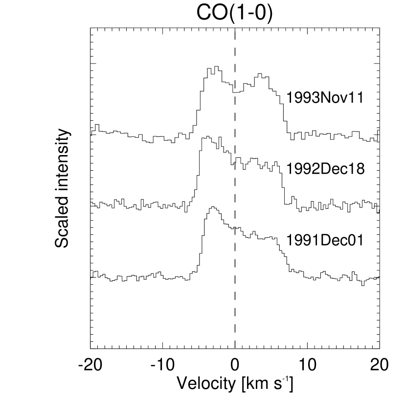
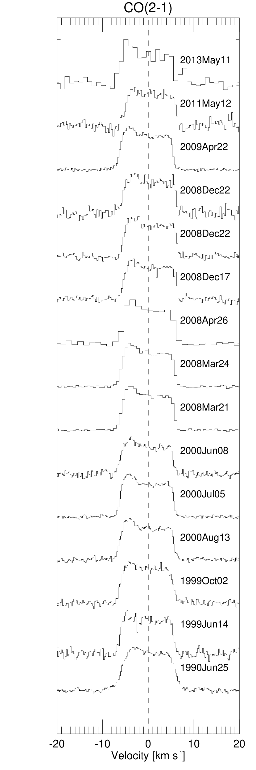
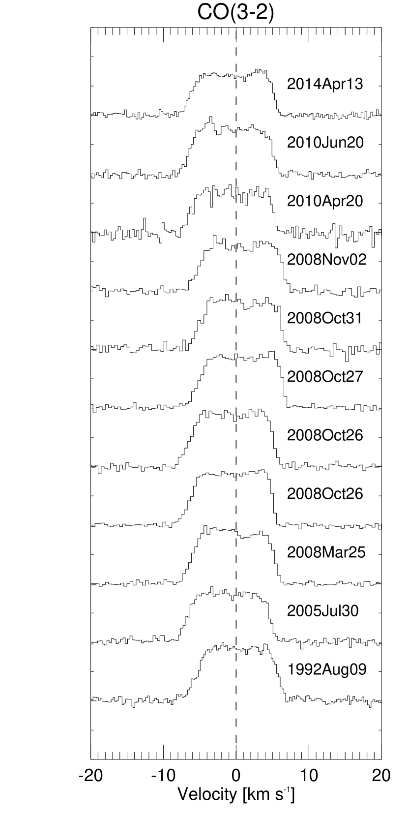
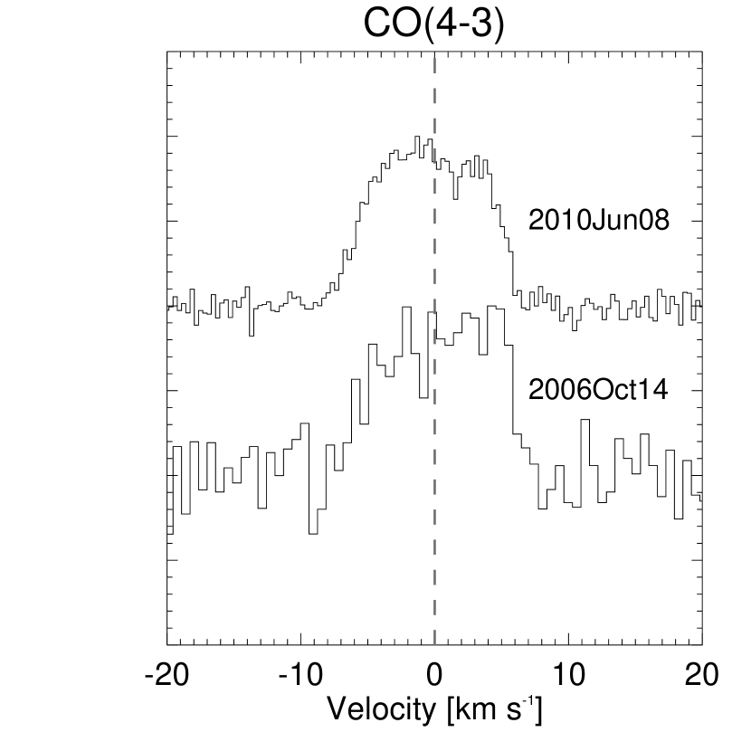
Figure 23: CO line emission from R Dor at different observing epochs: emission from $J=1-0,2-1,3-2$ measured by SEST in $1990-2000$, and from $J=2-1,3-2,4-3$ by APEX in $2005-2014$. The $y$-axis shows the line intensity at an arbitrary scale, chosen to optimise the visibility of the possible variations.

Appendix B Maser observations

With this paper we do not aim to study the maser excitation, but rather wish to report on the presence of the lines in the spectrum of R Dor. This is why all presented maser spectra in the main body of the paper are averages over all observations of that particular frequency. However, maser emission around AGB stars is known to significantly vary with time and we did not obtain all observations simultaneously. We therefore list the dates of observation for all maser lines in Table 5. Figure 24 presents the date-separated spectra of the maser lines observed on multiple days with significant S/N. We do not discuss any differences or implications of these in this paper. We note that we did not consider variations in those masers observed on consecutive days. If so wished, reduced spectra for separate dates of the other, much weaker, masers can be provided upon request.

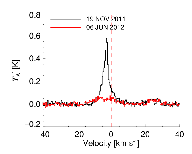
(a) SiO, $v=2$ ($J=6-5$) at 256.9 GHz

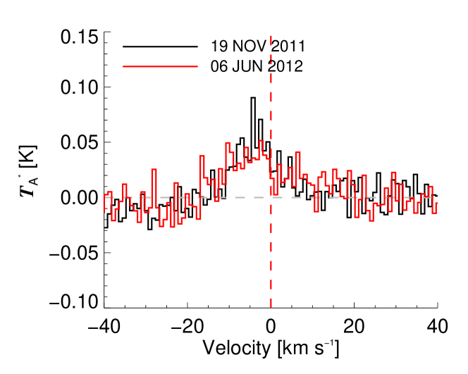
(b) SiO, $v=1$ ($J=6-5$) at 258.7 GHz

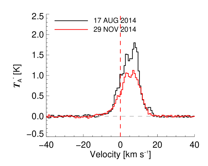
(c) SiO, $v=1$ ($J=7-6$) at 301.8 GHz

Figure 24: Maser variability in our survey data. The rest frequency of each line agrees with a 0 km s^-1 velocity in these plots.

Table 5: Observation dates for all maser lines in the survey, ordered according to increasing rest frequency.

Molecule	Transition	Frequency	Observation date
		(MHz)
30SiO, $v=2$	$4-3$	167160.943	22, 23 NOV 2015
30SiO, $v=1$	$4-3$	168323.353	22, 23 NOV 2015
SiO, $v=3$	$4-3$	170070.348	22, 23 NOV 2015
29SiO, $v=1$	$4-3$	170328.321	22, 23 NOV 2015
SiO, $v=2$	$4-3$	171275.165	22, 23 NOV 2015
SiO, $v=1$	$4-3$	172481.117	22, 23 NOV 2015
H2O	$3_{1,2}-2_{2,0}$	183310.087	22, 23 NOV 2015
30SiO, $v=2$	$5-4$	208946.055	22, 23 NOV 2015
SiO, $v=4$	$5-4$	211077.906	18 AUG 2014
SiO, $v=3$	$5-4$	212582.550	18 AUG 2014
SiO, $v=2$	$5-4$	214088.575	18 AUG 2014
SiO, $v=1$	$5-4$	215596.018	15 MAY 2011
H2O, $v_{2}=1$	$5_{5,0}-6_{4,3}$	232686.700	03 SEP 2011
SiO, $v=5$	$6-5$	251481.622	29 JUN 2015
30SiO, $v=1$	$6-5$	252471.372	29 JUN 2015
29SiO, $v=2$	$6-5$	253703.479	30 JUN 2015
29SiO, $v=1$	$6-5$	255478.495	30 JUN 2015
SiO, $v=2$	$6-5$	256898.396	19 NOV 2011,
			06 JUN 2012
SiO, $v=1$	$6-5$	258707.324	19 NOV 2011,
			06 JUN 2012
H2O, $v_{2}=2$	$6_{5,2}-7_{4,3}$	268149.117	13 JUN 2012,
			22 NOV 2012
H2O, $v_{2}=1$	$6_{6,1}-7_{5,2}$	293664.491	25 NOV 2011
29SiO, $v=3$	$7-6$	293907.859	25 NOV 2011
H2O, $v_{2}=1$	$6_{6,0}-7_{5,3}$	297439.276	25 NOV 2011
SiO, $v=3$	$7-6$	297595.467	25 NOV 2011
29SiO, $v=1$	$7-6$	298047.637	25 NOV 2011
SiO, $v=2$	$7-6$	299703.909	25 NOV 2011
SiO, $v=1$	$7-6$	301814.332	17 AUG 2014,
			29 NOV 2014
H2O	$10_{2,9}-9_{3,6}$	321225.677	24 NOV 2011
29SiO, $v=3$	$8-7$	335880.695	23 NOV 2011
30SiO, $v=1$	$8-7$	336603.002	23 NOV 2011
SiO, $v=4$	$8-7$	337687.290	23 NOV 2011
29SiO, $v=2$	$8-7$	338245.183	23 NOV 2011
SiO, $v=3$	$8-7$	340094.734	22 NOV 2011,
			27 JUN 2015
29SiO, $v=1$	$8-7$	340611.884	22 NOV 2011,
			27 JUN 2015
SiO, $v=2$	$8-7$	342504.383	11 NOV 2011,
			26, 27 JUN 2015
SiO, $v=1$	$8-7$	344916.332	11 NOV 2011,
			26, 27 JUN 2015
u	?	$\sim$354200	01 SEP 2011
			09 JUN 2016

Appendix C APEX survey data

We provide a complete overview of the survey in Table LABEL:tbl:lineID and Fig. 25.

To facilitate a direct comparison to the spectrum of IK Tau, Fig. 25 also shows the IRAM 30 m observations (in orange) of Velilla Prieto et al. (2017). We multiply the IK Tau spectrum with a factor $A$ to account for the difference in distance ($d$) and mass-loss rate ($\dot{M}$) between the two targets, and for the frequency-dependent difference in point-source sensitivity ($\sigma_{\nu}$) between the two telescopes:

$$A=\frac{\dot{M}_{\rm RDor}}{\dot{M}_{\rm IKTau}}\times\left(\frac{d_{\rm RDor}}{d_{\rm IKTau}}\right)^{-2}\times\left(\frac{\sigma_{\nu,\mathrm{APEX}}}{\sigma_{\nu,\mathrm{IRAM}}}\right)^{-1}=0.65\times\left(\frac{\sigma_{\nu,\mathrm{APEX}}}{\sigma_{\nu,\mathrm{IRAM}}}\right)^{-1}.$$ (4)

The distances and mass-loss rates are those reported by Maercker et al. (2016). The point-source sensitivities $\sigma_{\nu,\mathrm{APEX}}$ are those listed in Sect. 2; the values for $\sigma_{\nu,\mathrm{IRAM}}$ are taken from Velilla Prieto et al. (2017).

1]

Table 6: Overview of lines in the APEX survey of R Dor. The columns list the line number $N_{\mathrm{line}}$, the molecule, the transition, the theoretical rest frequency, the energy of the upper level of the transition, a reference to the catalogue used for the identification, the velocity resolution at which the identification was made, the minimum and maximum velocities of the line, $\varv_{\mathrm{min}}$ and $\varv_{\mathrm{max}}$ (w.r.t. the line center), the peak flux value, the integrated flux value over thelisted $\varv$-range, and remarks.Catalogues are (1) CDMS and (2) JPL

$N_{\mathrm{line}}$	Molecule	Transition	$\nu_{\mathrm{lab}}$	$E_{\mathrm{up}}/k$	Cat.	$\Delta\varv$	$\varv_{\mathrm{min}}$	$\varv_{\mathrm{max}}$	Peak	$I$	Remarks
			(MHz)	(K)		(km s-1)			(K)	(K km s-1)
1	SO2	$18_{2,16}-18_{1,17}$	160342.990	170.8	1	2.24	-6.9	5.8	0.02	0.19
2	Im(SiO)	$4-3$	160513.000	170.5	1	2.24	-24.8	15.5	0.04	0.31	Intensity at 2% of signal intensity.
3	TiO2?	$14_{9,5}-15_{8,8}$	160600.033	165.3	1	2.24	-7.0	11.6	0.01	0.03	Tentative.
4	SO2	$10_{0,10}-9_{1,9}$	160827.880	49.7	1	2.24	-5.8	8.4	0.03	0.25
5	Si18O	$4-3$	161404.881	19.4	1	2.23	-9.1	10.0	0.04	0.38
6	Im(SiO, $v=1$)	$4-3$	161719.900			2.22	-20.9	16.5	0.01	0.12	Intensity at 2% of signal intensity.
7	34SO2	$10_{0,10}-9_{1,9}$	162020.376	49.5	1	2.22	-13.6	13.6	0.01	0.07
8	Im(SiO,$v=2$)	$4-3$	162926.500			2.21	-11.2	11.8	0.06	0.42	Intensity at 2% of signal intensity.
9	SO2	$18_{2,16}-17_{3,15}$	163119.379	170.8	1	2.21	-6.5	7.3	0.01	0.08
10	SiS?	$9-8$	163376.785	39.2	1	2.20	-8.1	18.9	0.01	0.05	Tentative.
11	SO2	$14_{1,13}-14_{0,14}$	163605.533	101.8	1	2.20	-16.4	6.5	0.02	0.18
12	SO2?	$9_{4,6}-10_{3,7}$	165123.635	80.6	1	2.18	-6.8	8.1	0.01	0.02	Tentative.
13	SO2	$5_{2,4}-5_{1,5}$	165144.651	23.6	1	2.18	-14.1	3.9	0.01	0.05
14	SO2	$7_{1,7}-6_{0,6}$	165225.451	27.1	1	2.18	-6.1	11.3	0.02	0.19
15	30SiO, $v=2$	$4-3$	167160.943	3498.9	1	2.15	-8.4	10.5	0.01	0.11	Possible blend with Si17O.
16	Si17O	$4-3$	167171.984	20.1	1	2.15	-8.1	11.4	0.03	0.21	Possible blend with 30SiO, $v=2$.
17	SO18O?	$9_{4,6}-10_{3,7}$	168012.745	77.5	1	2.14	-4.4	12.0	0.01	0.05	Tentative.
18	30SiO, $v=1$	$4-3$	168323.353	1768.0	1	2.14	-9.5	8.5	0.04	0.32
19	30SiO	$4-3$	169486.872	20.3	1	2.12	-10.8	10.4	0.48	3.95
20	SiO, $v=3$	$4-3$	170070.348	5276.5	1	2.12	-8.9	8.5	0.79	4.59
21	29SiO, $v=1$	$4-3$	170328.321	1778.5	1	2.11	-10.3	7.3	0.10	0.69
22	SiO, $v=2$	$4-3$	171275.165	3541.0	1	2.10	-11.8	17.1	7.75	49.30
23	29SiO	$4-3$	171512.796	20.6	1	2.10	-12.8	8.7	0.92	7.33
24	Im(H2O)	$3_{1,2}-2_{2,0}$	171690.000			2.10	-11.3	8.0	0.01	0.09	Intensity at 0.3% of signal intensity.
25	SO	$4_{4}-3_{3}$	172181.403	33.8	1	2.09	-6.1	4.4	0.11	0.79
26	SiO, $v=1$	$4-3$	172481.117	1789.8	1	2.09	-23.8	13.8	0.26	2.66
27	H13CN	$2-1$	172677.851	12.4	1	2.08	-8.8	10.5	0.03	0.29
28	u	$?$	173514.000			2.07	-6.6	6.7	0.06	0.42
29	SiO	$4-3$	173688.238	20.8	1	2.07	-10.8	13.7	2.25	16.93
30	34SO2	$18_{2,16}-17_{3,15}$	174850.249	170.3	1	2.06	-5.4	9.9	0.01	0.06
31	SO2	$7_{2,6}-7_{1,7}$	175275.721	35.5	1	2.05	-9.2	8.9	0.03	0.19
32	34SO	$4_{5}-3_{4}$	175352.766	24.0	1	2.05	-21.4	13.4	0.02	0.14
33	HCN, $v_{2}=1$?	$2_{-1}-1_{1}$	177238.656	1037.1	1	2.03	-15.1	6.4	0.01	0.07	Tentative.
34	HCN	$2-1$	177261.111	12.8	1	2.03	-13.2	13.4	0.27	2.52
35	Im(30SiO)	$4-3$	178518.000			2.02	-4.4	18.6	0.03	0.21	Intensity at 5% of signal intensity.
36	SO	$4_{5}-3_{4}$	178605.403	24.4	1	2.01	-8.7	9.9	0.22	1.79
37	H2O	$3_{1,2}-2_{2,0}$	183310.087	204.7	2	1.96	-8.4	6.2	8.56	56.78	Maser.
38	Im(29SiO)	$4-3$	183488.000			2.45	-9.6	12.9	0.25	1.99	Intensity at 20% of signal intensity.
39	Im(SiO,$v=2$)	$4-3$	183727.000			1.96	-7.5	10.0	0.69	3.08	Intensity at 7% of signal intensity.
40	TiO2?	$26_{4,22}-26_{3,23}$	184254.593	281.5	1	5.86	-1.3	18.9	0.08	0.38	Tentative.
41	TiO2?	$30_{5,25}-30_{4,26}$	185887.601	375.8	1	5.81	-7.3	10.2	0.02	0.23	Tentative.
42	PN?	$4-3$	187953.263	22.6	1	3.83	-31.5	11.7	0.02	0.31	Tentative. Detection claimed from stacked spectrum.
43	SO2	$9_{2,8}-9_{1,9}$	188654.973	51.0	1	2.38	-8.5	8.4	0.03	0.22
44	u	$?$	189362.000			1.90	-12.5	10.3	0.02	0.16
45	SO2	$2_{2,0}-1_{1,1}$	192651.020	12.6	1	1.87	-6.2	8.0	0.02	0.11
46	SO2	$9_{1,9}-8_{0,8}$	193609.490	42.0	1	1.86	-5.3	7.6	0.06	0.42
47	SO2	$22_{3,19}-22_{2,20}$	195320.700	257.8	1	1.84	-5.7	5.5	0.02	0.16
48	PO	$5_{1,5,5}-4_{1,4,4}$	196305.920	25.1	1	1.83	-5.6	9.5	0.01	0.06
49	PO	$5_{1,5,4}-4_{1,4,3}$	196319.816	25.2	1	1.83	-6.4	8.7	0.02	0.15
50	PO	$5_{1,5,5}-4_{1,4,4}$	196500.222	25.2	1	1.83	-4.1	12.4	0.02	0.08
51	PO	$5_{1,5,4}-4_{1,4,3}$	196518.400	25.2	1	1.83	-11.4	6.1	0.01	0.05
52	SO2	$20_{3,17}-20_{2,18}$	197142.180	217.2	1	1.82	-9.3	5.9	0.03	0.23
53	29Si18O?	$5-4$	199031.722	28.7	1	3.62	-11.3	3.3	0.01	0.02	Tentative.
54	SO2	$24_{3,21}-24_{2,22}$	200287.421	302.4	1	1.80	-7.8	9.0	0.02	0.14
55	SO2	$16_{1,15}-16_{0,16}$	200809.180	130.7	1	1.79	-14.5	11.8	0.03	0.27
56	Si18O	$5-4$	201751.489	29.0	1	1.78	-5.7	5.3	0.07	0.51
57	34SO	$5_{4}-4_{3}$	201846.480	38.1	1	2.23	-9.2	14.1	0.01	0.07
58	SO2	$12_{0,12}-11_{1,11}$	203391.550	70.1	1	1.77	-15.8	10.5	0.07	0.59
59	u	$?$	204008.000			2.20	-8.8	5.6	0.01	0.09
60	SO2	$18_{3,15}-18_{2,16}$	204246.761	180.6	1	1.76	-12.2	7.7	0.04	0.31
61	SO2	$11_{2,10}-11_{1,11}$	205300.570	70.2	1	1.75	-6.3	6.4	0.04	0.25
62	TiO2?	$19_{5,15}-19_{4,16}$	206049.296	166.5	1	1.75	-10.5	9.2	0.01	0.09	Tentative.
63	SO	$5_{4}-4_{3}$	206176.005	38.6	1	1.74	-6.0	6.6	0.17	1.33
64	SO2	$3_{2,2}-2_{1,1}$	208700.336	15.3	1	1.72	-9.4	5.4	0.01	0.09
65	Si17O	$5-4$	208960.000	30.1	1	1.72	-11.6	7.9	0.04	0.35
66	SiO, $v=4$?	$5-4$	211077.906	7004.5	1	3.41	-6.1	11.1	0.02	0.11	Tentative.
67	30SiO	$5-4$	211853.471	30.5	1	0.99	-19.7	15.2	0.70	5.34
68	SiO, $v=3$	$5-4$	212582.550	5286.7	1	3.38	-10.1	22.8	0.04	0.43
69	SO2	$26_{3,23}-26_{2,24}$	213068.427	350.8	1	2.11	-25.7	10.6	0.02	0.14
70	SiO, $v=2$?	$5-4$	214088.575	3552.0	1	3.36	-12.8	21.2	0.01	0.15	Tentative.
71	29SiO	$5-4$	214385.752	30.9	1	2.10	-12.7	11.7	1.02	7.60
72	SO2	$16_{3,13}-16_{2,14}$	214689.394	147.8	1	2.09	-9.5	19.0	0.04	0.33
73	SO2?	$17_{6,12}-18_{5,13}$	214728.285	229.0	1	2.09	-15.5	15.5	0.01	0.02	Tentative.
74	SO	$5_{5}-4_{4}$	215220.653	44.1	1	2.09	-12.0	13.0	0.21	1.67
75	SiO, $v=1$	$5-4$	215596.018	1800.2	1	2.09	-13.2	25.9	1.10	8.53
76	34SO	$5_{6}-4_{5}$	215839.920	34.4	1	2.08	-10.0	14.6	0.03	0.26
77	SO2	$22_{2,20}-22_{1,21}$	216643.304	248.4	1	2.08	-6.4	19.5	0.05	0.40
78	SiO	$5-4$	217104.919	31.3	1	2.07	-26.3	29.3	3.04	24.54
79	SO	$5_{6}-4_{5}$	219949.442	35.0	1	2.04	-29.9	8.5	0.36	3.07
80	13CO	$2-1$	220398.684	15.9	1	2.04	-24.0	18.6	0.16	1.41
81	SO2	$11_{1,11}-10_{0,10}$	221965.220	60.4	1	2.03	-23.3	8.3	0.09	0.72
82	SO2	$20_{2,18}-19_{3,17}$	224264.814	207.8	1	2.01	-20.7	15.7	0.02	0.14
83	SO2	$13_{2,12}-13_{1,13}$	225153.704	93.0	1	2.00	-23.8	14.7	0.06	0.49
84	u	$?$	225998.000			3.18	-8.0	13.9	0.01	0.12
85	SO2	$14_{3,11}-14_{2,12}$	226300.027	119.0	1	1.99	-17.7	11.7	0.06	0.46
86	CO	$2-1$	230538.000	16.6	1	1.95	-38.4	9.4	2.90	30.98
87	H2O, $v_{2}=1$	$5_{5,0}-6_{4,3}$	232686.700	3461.9	2	1.93	-16.2	13.9	0.04	0.25
88	SO2	$28_{3,25}-28_{2,26}$	234187.057	403.0	1	3.07	-27.7	4.6	0.03	0.35
89	PN?	$5-4$	234935.695	33.8	1	3.06	-30.2	24.5	0.02	0.12	Tentative. Detection claimed from stacked spectrum.
90	SO2	$4_{2,2}-3_{1,3}$	235151.720	19.0	1	1.91	-10.7	11.5	0.04	0.18
91	SO2	$16_{1,15}-15_{2,14}$	236216.687	130.7	1	1.90	-16.0	13.7	0.07	0.45
92	SO2	$12_{3,9}-12_{2,10}$	237068.833	94.0	1	1.90	-25.5	12.6	0.06	0.46
93	TiO2?	$30_{7,23}-30_{6,24}$	238050.296	395.3	1	4.53	-7.6	11.3	0.01	0.08	Tentative.
94	PO	$6_{-1,6,6}-5_{1,5,5}$	239948.982	36.7	1	1.87	-25.4	15.1	0.03	0.23
95	PO	$6_{-1,6,5}-5_{1,5,4}$	239958.101	36.7	1	1.87	-14.0	26.5	0.03	0.23
96	PO	$6_{1,6,6}-5_{-1,5,5}$	240141.059	36.7	1	1.87	-32.9	16.9	0.03	0.36
97	PO	$6_{1,6,5}-5_{-1,5,4}$	240152.528	36.7	1	1.87	-18.6	31.2	0.03	0.36
98	SO2	$18_{1,17}-18_{0,18}$	240942.792	163.1	1	1.87	-20.7	21.1	0.05	0.40
99	SO2	$5_{2,4}-4_{1,3}$	241615.797	23.6	1	1.86	-19.1	15.3	0.04	0.33
100	Si18O	$6-5$	242094.982	40.7	1	1.86	-20.5	9.3	0.10	0.83
101	NaCl, $v=2$?	$19-18$	243574.069	1151.2	1	2.95	-33.6	30.6	0.01	0.12	Tentative. Variability seen between two observing dates.
102	SO2	$14_{0,14}-13_{1,13}$	244254.218	93.9	1	1.84	-13.8	17.8	0.13	1.13
103	TiO2?	$23_{6,18}-23_{5,19}$	244476.538	241.6	1	4.41	-14.7	9.2	0.01	0.10	Tentative.
104	34SO2	$14_{0,14}-13_{1,13}$	244481.517	93.5	1	1.84	-9.4	14.6	0.01	0.09
105	SO2	$26_{3,23}-25_{4,22}$	245339.233	350.8	1	1.83	-11.3	13.6	0.02	0.11
106	SO2	$10_{3,7}-10_{2,8}$	245563.422	72.7	1	1.83	-15.4	14.7	0.05	0.45
107	Im(SiO)	$6-5$	246486.000			1.82	-17.6	16.7	0.07	0.47	Intensity at 2% of signal intensity.
108	34SO	$6_{5}-5_{4}$	246663.470	49.9	1	1.82	-22.3	14.3	0.02	0.18
109	SO2	$31_{9,23}-32_{8,24}$	247169.768	654.5	1	1.82	-20.2	32.0	0.01	0.19
110	NaCl?	$19-18$	247239.733	118.7	1	2.91	-17.2	26.5	0.01	0.17	Tentative.
111	SO2	$15_{2,14}-15_{1,15}$	248057.402	119.3	1	1.81	-15.1	9.6	0.05	0.37
112	Si17O	$6-5$	250744.695	42.1	1	1.79	-19.0	24.7	0.06	0.49
113	SO2	$13_{1,13}-12_{0,12}$	251199.675	82.2	1	1.79	-7.0	18.2	0.10	0.81
114	SO2	$8_{3,5}-8_{2,6}$	251210.585	55.2	1	1.79	-7.5	6.1	0.04	0.26
115	SiO, $v=5$	$6-5$	251481.622	8717.3	1	1.43	-7.2	11.5	0.02	0.10
116	Im(SO2)	$11_{3,9}-11_{2,10}$	251744.000			1.43	-9.2	6.8	0.02	0.05	Intensity at 23% of signal intensity.
117	SO	$6_{5}-5_{4}$	251825.770	50.7	1	1.79	-17.7	10.9	0.27	2.21
118	30SiO, $v=1$	$6-5$	252471.372	1790.2	1	1.42	-14.0	5.8	0.03	0.11
119	34SO	$6_{6}-5_{5}$	253207.017	55.7	1	1.78	-14.9	8.5	0.03	0.23
120	29SiO, $v=2$	$6-5$	253703.479	3541.9	1	1.77	-17.0	12.7	0.03	0.18
121	30SiO	$6-5$	254216.656	42.7	1	1.77	-17.2	12.7	0.95	6.98
122	SO2	$6_{3,3}-6_{2,4}$	254280.536	41.4	1	1.77	-21.8	12.9	0.07	0.60
123	29SiO, $v=1$	$6-5$	255478.495	1801.0	1	1.76	-24.2	16.0	0.05	0.18
124	SO2	$4_{3,1}-4_{2,2}$	255553.302	31.3	1	1.76	-11.0	10.8	0.02	0.03
125	SO2	$5_{3,3}-5_{2,4}$	256246.945	35.9	1	1.75	-19.1	11.8	0.03	0.31
126	34SO	$6_{7}-5_{6}$	256877.809	46.7	1	1.75	-12.2	11.6	0.04	0.28
127	SiO, $v=2$	$6-5$	256898.396	3564.3	1	1.75	-20.9	11.8	0.19	1.36
128	SO2	$7_{3,5}-7_{2,6}$	257099.966	47.8	1	1.75	-16.4	9.5	0.04	0.34
129	29SiO	$6-5$	257255.213	43.2	1	1.75	-28.2	20.6	1.21	9.31
130	SO	$6_{6}-5_{5}$	258255.826	56.5	1	1.74	-25.9	14.5	0.33	2.57
131	SO2	$32_{4,28}-32_{3,29}$	258388.716	531.1	1	1.74	-17.8	12.8	0.03	0.25
132	SiO, $v=1$	$6-5$	258707.324	1812.6	1	1.74	-21.5	21.6	0.05	0.78
133	SO2	$9_{3,7}-9_{2,8}$	258942.199	63.5	1	1.74	-13.1	9.8	0.04	0.39
134	H13CN	$3-2$	259011.798	24.9	1	1.74	-24.9	7.8	0.07	0.57
135	SO2	$30_{4,26}-30_{3,27}$	259599.448	471.5	1	1.73	-9.3	6.5	0.02	0.16
136	SiO	$6-5$	260518.009	43.8	1	1.73	-13.8	14.3	4.26	31.72
137	TiO2?	$34_{5,29}-34_{4,30}$	261127.076	474.3	1	4.13	-13.9	9.0	0.01	0.07	Tentative.
138	SO	$6_{7}-5_{6}$	261843.721	47.6	1	1.72	-10.7	11.2	0.50	3.87
139	Data	$?$	262000.000			2.75	-22.9	22.9	0.01	0.04	Data issue.
140	SO2	$11_{3,9}-11_{2,10}$	262256.906	82.8	1	1.71	-9.9	20.4	0.07	0.54
141	H2O, $v_{2}=1$	$7_{7,0}-8_{6,3}$	263451.357	4474.5	2	1.71	-18.4	23.4	0.02	0.26
142	SO2	$30_{3,27}-30_{2,28}$	263543.953	459.0	1	1.71	-9.6	12.0	0.03	0.17
143	Im(29SiO)	$6-5$	263780.000			1.70	-20.1	15.5	0.07	0.47	Intensity at 4% of signal intensity.
144	HCN	$3-2$	265886.400	25.5	1	1.69	-20.9	9.7	0.71	5.82
145	SO2	$13_{3,11}-13_{2,12}$	267537.451	105.8	1	1.68	-13.2	15.1	0.05	0.43
146	SO2	$28_{4,24}-28_{3,25}$	267719.840	415.9	1	1.68	-15.3	17.0	0.06	0.35
147	Im(29SiO)	$6-5$	267745.000			1.68	-10.1	10.0	0.04	0.33	Intensity at 5% of signal intensity.
148	u	$?$	267993.000			1.68	-4.0	6.0	0.02	0.09
149	H2O, $v_{2}=2$	$6_{5,2}-7_{4,3}$	268149.117	6039.0	2	1.68	-12.5	21.7	0.04	0.33
150	Im(SO2)	$16_{0,16}-15_{1,15}$	270537.000			1.66	-18.5	26.2	0.03	0.34	Intensity at 15% of signal intensity.
151	TiO2?	$26_{7,19}-26_{6,20}$	271311.202	310.7	1	3.98	-10.5	13.4	0.01	0.11	Tentative.
152	SO2	$7_{2,6}-6_{1,5}$	271529.014	35.5	1	1.32	-13.9	19.2	0.05	0.40
153	TiO2?	$22_{1,21}-22_{0,22}$	271566.716	180.5	1	3.97	-3.5	12.8	0.01	0.06	Tentative.
154	SiS?	$15-14$	272243.052	104.5	1	2.64	-16.4	26.7	0.02	0.16	Tentative.
155	Im(SO2)	$17_{3,15}-17_{2,16}$	273258.000			1.32	-14.3	12.1	0.04	0.27	Intensity at 54% of signal intensity.
156	u	$?$	273284.000			1.32	-18.6	12.1	0.07	0.51
157	SO2	$17_{2,16}-17_{1,17}$	273752.822	149.2	1	1.31	-9.1	9.7	0.04	0.28
158	SO2	$15_{3,13}-15_{2,14}$	275240.184	132.5	1	1.31	-13.5	15.4	0.06	0.53
159	TiO2?	$27_{4,24}-27_{3,25}$	276437.905	292.7	1	3.90	-16.5	8.0	0.00	-0.01	Tentative.
160	TiO2?	$27_{16,12}-28_{15,13}$	276827.330	555.0	1	3.90	-10.5	13.2	0.01	0.06	Tentative.
161	29Si18O	$7-6$	278627.547	53.3	1	2.58	-7.7	5.4	0.01	0.07
162	u	$?$	280051.000			1.50	-5.5	6.3	0.02	0.08
163	SO2	$26_{4,22}-26_{3,23}$	280807.246	364.3	1	1.28	-22.3	19.9	0.04	0.40
164	SO2	$36_{4,32}-36_{3,33}$	281688.931	662.1	1	1.28	-12.0	14.4	0.03	0.17
165	SO2	$15_{1,15}-14_{0,14}$	281762.600	107.4	1	1.28	-23.1	15.2	0.16	1.32
166	PN?	$6-5$	281914.205	47.4	1	2.55	-6.1	5.6	0.02	0.09	Tentative. Detection claimed from stacked spectrum.
167	SO2	$6_{2,4}-5_{1,5}$	282036.566	29.2	1	1.28	-9.8	18.5	0.03	0.16
168	SO2	$20_{1,19}-20_{0,20}$	282292.806	198.9	1	1.27	-12.8	22.7	0.04	0.28
169	Si18O	$7-6$	282434.716	54.2	1	1.27	-9.7	19.4	0.12	0.95
170	Im(30SiO)	$7-6$	283425.000			1.48	-9.6	11.4	0.03	0.19	Intensity at 3% of signal intensity.
171	SO2	$16_{0,16}-15_{1,15}$	283464.769	121.0	1	1.27	-26.9	11.2	0.15	1.23
172	u	$?$	283535.000			1.27	-6.6	11.6	0.02	0.14
173	PO	$7_{1,7,7}-6_{-1,6,6}$	283586.835	50.3	1	2.54	-22.9	14.3	0.04	0.44
174	PO	$7_{1,7,6}-6_{-1,6,5}$	283593.186	50.3	1	2.54	-16.2	21.0	0.04	0.44
175	PO	$7_{-1,7,7}-6_{1,6,6}$	283777.610	50.3	1	2.54	-50.6	27.4	0.03	0.45
176	PO	$7_{-1,7,6}-6_{1,6,5}$	283785.419	50.3	1	2.54	-42.3	35.6	0.03	0.45
177	SO18O	$19_{7,13}-20_{6,14}$	285106.318	282.4	1	2.42	-13.2	22.2	0.01	0.03	Weak.
178	SO18O	$19_{7,12}-20_{6,15}$	285109.824	282.4	1	2.42	-9.5	25.9	0.01	0.03	Weak.
179	SO2	$17_{3,15}-17_{2,16}$	285743.600	162.9	1	1.26	-31.1	12.2	0.06	0.41
180	Im(SO)	$7_{7}-6_{6}$	286714.000			1.25	-32.3	9.0	0.16	1.08	Intensity at 21% of signal intensity.
181	TiO2?	$34_{8,26}-34_{7,27}$	286802.035	506.8	1	3.76	-4.9	14.5	0.02	0.15	Tentative.
182	Im(29SiO)	$7-6$	287880.000			1.25	-30.8	15.6	0.25	2.09	Intensity at 12% of signal intensity.
183	SO18O	$19_{3,17}-19_{2,18}$	288269.800	186.8	1	1.25	-11.5	19.7	0.02	0.21
184	SO18O	$25_{4,21}-25_{3,22}$	288296.707	322.1	1	1.25	-16.5	13.7	0.10	0.51
185	SO18O	$35_{10,26}-36_{9,27}$	288481.517	786.3	1	1.25	-4.1	15.1	0.02	0.15
186	SO2	$18_{1,17}-17_{2,16}$	288519.996	163.1	1	1.25	-13.8	20.9	0.09	0.54
187	29Si17O?	$7-6$	288718.636	55.4	1	1.25	-8.5	11.1	0.02	0.08	Tentative.
188	Im(SiO)	$7-6$	291073.000			1.24	-17.9	28.8	0.10	0.76	Intensity at 3% of signal intensity.
189	TiO2?	$20_{7,13}-20_{6,14}$	291163.340	207.0	1	2.47	-7.3	5.9	0.01	0.05	Tentative.
190	Si17O	$7-6$	292525.407	56.2	1	1.23	-7.7	8.8	0.06	0.49
191	Im(SiO, $v=1$)	$7-6$	293189.000			1.23	-12.3	15.7	0.08	0.64	Intensity at 12% of signal intensity.
192	H2O, $v_{2}=1$	$6_{6,1}-7_{5,2}$	293664.491	3933.6	2	1.23	-26.0	13.4	0.04	0.55
193	29SiO, $v=3$	$7-6$	293907.859	5280.1	1	1.22	-15.8	9.6	0.04	0.40
194	TiO2?	$33_{6,28}-33_{5,29}$	294442.979	451.9	1	3.67	-15.5	14.4	0.02	0.13	Tentative.
195	34SO	$7_{7}-6_{6}$	295396.334	69.9	1	1.22	-13.5	16.2	0.03	0.06
196	u	$?$	295629.000			2.33	-8.2	7.1	0.03	0.20
197	SO2	$26_{2,24}-26_{1,25}$	296168.675	340.6	1	1.21	-6.8	16.7	0.03	0.27
198	SO2	$24_{4,20}-24_{3,21}$	296535.422	316.6	1	1.21	-6.3	19.1	0.04	0.23	Possible blend with SO.
199	SO	$7_{6}-6_{5}$	296550.064	64.9	1	1.21	-12.3	8.5	0.38	2.85	Possible blend with SO2.
200	30SiO	$7-6$	296575.730	56.9	1	1.21	-29.7	13.7	0.94	6.72
201	u	$?$	297404.000			1.51	-16.0	13.7	0.03	0.34	Tentative: TiN at 297401.8 MHz.
202	H2O, $v_{2}=1$	$6_{6,0}-7_{5,3}$	297439.276	3933.6	2	1.21	-34.0	14.4	0.02	0.12
203	SiO, $v=3$	$7-6$	297595.467	5313.3	1	1.21	-13.1	23.2	0.03	0.26
204	TiO2?	$32_{6,26}-31_{7,25}$	297702.188	432.1	1	3.63	-12.3	13.3	0.02	0.19	Tentative.
205	29SiO, $v=1$	$7-6$	298047.637	1815.3	1	1.21	-18.9	26.0	0.02	0.23
206	34SO	$7_{8}-6_{7}$	298257.982	61.0	1	1.21	-31.7	23.5	0.04	0.46
207	u	$?$	298464.000			1.21	-13.2	11.6	0.03	0.12
208	SO2	$9_{2,8}-8_{1,7}$	298576.307	51.0	1	1.20	-12.4	14.3	0.07	0.41
209	Data	$/$	299035.000			2.31	-13.4	14.4	0.02	0.22	Data issue.
210	NaCl?	$23-22$	299145.700	172.4	1	2.41	-15.9	12.1	0.01	0.13	Tentative.
211	SO2	$19_{3,17}-19_{2,18}$	299316.818	197.0	1	1.20	-20.3	11.9	0.05	0.45
212	SiO, $v=2$	$7-6$	299703.909	3578.7	1	1.20	-12.6	12.2	0.73	2.84
213	29SiO	$7-6$	300120.480	57.6	1	1.20	-18.8	18.9	1.57	11.13
214	SO2	$32_{3,29}-32_{2,30}$	300273.418	518.7	1	1.20	-8.4	19.1	0.03	0.31
215	SO	$7_{7}-6_{6}$	301286.124	71.0	1	1.19	-17.0	13.8	0.44	3.46
216	SiO, $v=1$	$7-6$	301814.332	1827.1	1	1.19	-15.4	21.3	1.32	16.33
217	SO2	$19_{2,18}-19_{1,19}$	301896.629	182.6	1	1.19	-8.6	16.1	0.06	0.42
218	SO18O	$17_{2,16}-16_{2,15}$	303154.811	141.3	2	2.37	-11.0	13.6	0.02	0.19
219	SO18O	$18_{0,18}-17_{1,17}$	303475.791	143.4	2	2.37	-15.9	18.0	0.02	0.18
220	SiO	$7-6$	303926.812	58.3	1	1.18	-21.9	14.5	4.01	29.39
221	SO	$7_{8}-6_{7}$	304077.844	62.1	1	1.18	-29.3	29.0	0.61	4.74
222	Im(H2O, $v_{2}=1$)	$6_{6,1}-7_{5,2}$	305331.000			2.26	-3.2	10.5	0.02	0.10	Intensity at 50% of signal intensity.
223	SO2	$38_{4,34}-38_{3,35}$	307185.305	733.4	1	1.17	-9.7	7.7	0.02	0.16
224	PNO?	$25-24$	309423.503	193.1	1	2.33	-11.5	13.5	0.02	0.18	Tentative. No other transitions of PNO detected, but feature is real.
225	u	$?$	309449.000			1.16	-5.6	11.6	0.01	0.06
226	SO	$2_{2}-1_{2}$	309502.444	19.3	1	1.16	-17.5	9.4	0.02	0.05
227	SO2	$22_{4,18}-22_{3,19}$	312542.519	272.8	1	1.15	-23.8	13.3	0.05	0.32
228	SO2	$3_{3,1}-2_{2,0}$	313279.718	27.6	1	1.15	-11.0	9.6	0.05	0.27
229	SO2	$28_{3,25}-27_{4,24}$	313412.285	403.0	1	2.30	-14.6	10.0	0.02	0.03
230	SO2	$17_{1,17}-16_{0,16}$	313660.852	136.1	1	1.15	-19.6	9.9	0.26	2.12
231	SO2	$21_{3,19}-21_{2,20}$	316098.874	234.7	1	1.14	-18.0	17.8	0.07	0.66
232	29Si18O?	$8-7$	318419.436	68.8	1	1.41	-5.6	11.5	0.02	0.19	Tentative.
233	SO17O	$28_{3,26}-29_{0,29}$	318673.384	383.9	1	1.13	-13.2	16.7	0.05	0.39
234	u	$?$	319253.000			1.41	-9.4	13.1	0.02	0.08
235	SO2	$40_{5,35}-40_{4,36}$	319277.053	823.7	1	2.25	-12.2	10.8	0.03	0.27
236	SO2	$42_{5,37}-42_{4,38}$	319698.702	902.3	1	2.16	-6.7	12.9	0.03	0.25
237	u	$?$	320204.000			2.25	-21.3	18.8	0.06	0.52
238	Im(13CO)	$3-2$	320413.000			2.25	-13.7	16.1	0.04	0.26	Intensity at 7% of signal intensity.
239	H2O	$10_{2,9}-9_{3,6}$	321225.677	1861.2	2	1.12	-21.9	15.8	0.64	3.35	Maser.
240	SO2	$18_{0,18}-17_{1,17}$	321330.166	151.5	1	1.12	-15.6	22.0	0.17	1.48
241	PN?	$7-6$	328888.006	63.1	1	1.09	-6.3	6.3	0.03	0.17	Tentative. Detection claimed from stacked spectrum.
242	29Si17O?	$8-7$	329951.219	71.3	1	2.18	-11.3	3.9	0.02	0.12	Tentative.
243	13CO	$3-2$	330587.965	31.7	1	1.09	-7.5	7.1	0.42	3.91
244	SO2	$21_{2,20}-21_{1,21}$	332091.431	219.5	1	1.35	-4.6	3.7	0.05	0.32
245	u	$?$	332217.000			1.35	-16.9	8.6	0.05	0.21
246	Im(SO2)	$19_{1,19}-18_{0,18}$	332348.000			1.35	-9.3	5.3	0.04	0.29	Intensity at 18% of signal intensity.
247	Im(SO)	$8_{9}-7_{8}$	332472.000			1.35	-11.7	14.2	0.05	0.27	Intensity at 17% of signal intensity.
248	SO2	$4_{3,1}-3_{2,2}$	332505.242	31.3	1	1.35	-7.1	6.6	0.06	0.43
249	Im(CO)	$3-2$	333205.000			1.35	-11.2	8.7	0.07	0.63	Intensity at 5% of signal intensity.
250	34SO	$8_{7}-7_{6}$	333900.983	79.9	1	1.35	-17.9	18.7	0.04	0.38
251	Si17O	$8-7$	334301.470	72.2	1	1.35	-5.2	10.1	0.09	0.65
252	SO2	$8_{2,6}-7_{1,7}$	334673.353	43.1	1	1.34	-6.7	5.6	0.07	0.55
253	SiO, $v=5$?	$8-7$	335281.980	8747.0	1	2.15	-20.1	10.3	0.02	0.28	Tentative.
254	29SiO, $v=3$	$8-7$	335880.695	5296.2	1	1.34	-10.8	19.8	0.05	0.45
255	SO2	$23_{3,21}-23_{2,22}$	336089.228	276.0	1	1.34	-14.9	7.7	0.06	0.47
256	H2O, $v_{2}=1$	$5_{2,3}-6_{1,6}$	336227.941	2955.2	1	1.07	-17.6	9.3	0.05	0.25
257	30SiO, $v=1$	$8-7$	336603.002	1820.5	1	1.07	-12.6	10.7	1.03	5.27
258	SO2	$16_{7,9}-17_{6,12}$	336669.581	245.1	1	1.34	-2.9	4.7	0.03	0.11
259	TiO2?	$38_{5,33}-38_{4,34}$	337366.365	582.5	1	3.20	-7.4	3.6	0.02	0.06	Tentative.
260	34SO	$8_{8}-7_{7}$	337580.147	86.1	1	1.33	-7.0	6.8	0.05	0.33
261	SiO, $v=4$?	$8-7$	337687.290	7047.0	1	2.13	-8.8	5.2	0.01	0.04	Tentative.
262	29SiO, $v=2$	$8-7$	338245.183	3572.4	1	1.33	-10.2	20.5	0.05	0.70
263	SO2	$18_{4,14}-18_{3,15}$	338305.993	196.8	1	1.33	-15.3	17.5	0.05	0.25
264	SO2	$20_{1,19}-19_{2,18}$	338611.810	198.9	1	1.33	-20.2	15.8	0.11	0.98
265	30SiO	$8-7$	338930.058	73.2	1	1.06	-26.8	16.4	1.15	8.44
266	SO	$3_{3}-2_{3}$	339341.459	25.5		2.12	-9.4	14.1	0.02	0.17
267	34SO	$8_{9}-7_{8}$	339857.269	77.3		2.12	-6.8	11.4	0.03	0.31
268	CN	$3-2(A)$	340033.400	32.6	1	1.06	-8.0	29.6	0.02	0.15	Hyperfine structure. Frequency chosen for peak.
269	SiO, $v=3$	$8-7$	340094.734	5329.6	1	1.06	-9.4	25.8	0.04	0.36
270	CN	$3-2(B)$	340247.600	32.7	1	1.06	-38.5	10.1	0.03	0.29	Hyperfine structure. Frequency chosen for peak.
271	SO2	$28_{2,26}-28_{1,27}$	340316.406	391.8	1	2.11	-16.3	7.8	0.04	0.28
272	29SiO, $v=1$	$8-7$	340611.884	1831.7	1	2.11	-15.1	18.9	0.02	0.35
273	SO	$8_{7}-7_{6}$	340714.155	81.2	1	2.11	-11.9	16.8	0.46	3.86
274	SO2	$52_{14,38}-53_{13,41}$	341321.948	1744.9	1	2.02	-6.6	-75.9	0.00	0.00	Blend.
275	SO2	$53_{6,48}-52_{7,45}$	341323.306	1411.6	1	2.02	-5.4	-74.7	0.00	0.00	Blend.
276	SO2	$40_{4,36}-40_{3,37}$	341403.068	808.4	1	2.11	-11.0	7.9	0.03	0.22
277	SO2	$36_{5,31}-36_{4,32}$	341673.961	678.5	1	2.11	-3.3	5.1	0.03	0.15
278	SiO, $v=2$?	$8-7$	342504.383	3593.1	1	2.01	-11.6	17.7	0.02	0.11	Tentative.
279	SO2	$34_{3,31}-34_{2,32}$	342761.625	581.9	1	2.10	-12.3	27.4	0.03	0.28
280	29SiO	$8-7$	342980.847	74.1	1	2.10	-20.2	25.6	1.54	11.46
281	SO	$8_{8}-7_{7}$	344310.612	87.5	1	2.09	-19.0	13.9	0.49	4.05
282	AlO?	$9-8(components)$	344433.400	82.7	2	2.09	-15.1	9.6	0.01	0.05	Tentative.
283	SO18O	$14_{4,10}-14_{3,11}$	344873.823	129.6	1	2.09	-17.6	15.1	0.02	0.07
284	SiO, $v=1$	$8-7$	344916.332	1843.6	1	2.09	-17.3	18.5	0.05	0.69
285	SO2	$13_{2,12}-12_{1,11}$	345338.538	93.0	1	2.08	-13.2	13.6	0.20	1.75	Blend with H13CN.
286	H13CN	$4-3$	345339.769	41.4	1	2.08	-12.2	14.6	0.20	1.75	Blend with SO2.
287	Im(13CO)	$3-2$	345410.000			2.08	-8.6	5.1	0.03	0.29	Intensity at 8% of signal intensity.
288	Im(HCN)	$4-3$	345496.000			1.30	-14.6	13.2	0.04	0.23	Intensity at 7% of signal intensity.
289	CO	$3-2$	345795.990	33.2	1	2.08	-22.9	14.9	3.64	41.55
290	SO17O	$30_{3,28}-31_{0,31}$	346334.091	436.1	1	1.04	-10.7	5.8	0.03	0.12
291	SO18O	$13_{4,9}-13_{3,10}$	346392.655	117.4	1	2.08	-13.9	8.9	0.02	0.25
292	SO2	$16_{4,12}-16_{3,13}$	346523.878	164.5	1	2.08	-16.0	17.4	0.61	5.10	Blend with SO.
293	SO	$8_{9}-7_{8}$	346528.481	78.8	1	2.08	-12.0	21.4	0.61	5.10	Blend with SO2.
294	SO2	$19_{1,19}-18_{0,18}$	346652.169	168.1	1	2.08	-7.5	11.8	0.22	1.76
295	SiO	$8-7$	347330.581	75.0	1	2.07	-20.8	26.6	4.79	36.91
296	SO2	$24_{2,22}-23_{3,21}$	348387.800	292.7	1	1.46	-8.8	15.3	0.06	0.44
297	SO2, $v_{2}=1$	$69_{9,61}-70_{6,64}$	349977.759	3176.9	1	1.28	-6.9	10.6	0.07	0.22
298	SO2	$5_{3,3}-4_{2,2}$	351257.223	35.9	1	2.05	-12.9	21.5	0.06	0.54
299	SO2	$14_{4,10}-14_{3,11}$	351873.873	135.9	1	2.04	-6.3	23.0	0.07	0.56
300	Im(SO)	$8_{8}-7_{7}$	352689.000			2.04	-14.5	11.7	0.01	-0.11	Intensity at 8% of signal intensity.
301	Im(29SiO)	$8-7$	354018.000	34.0	1	2.03	-8.3	12.8	0.09	0.50	Intensity at 5 % of signal intensity.
302	u	$?$	354195.000			2.03	-5.6	6.2	0.82	4.73	Unknown maser. Tentatively identified as H2SiO.
303	HCN	$4-3$	354505.477	42.5	1	2.03	-21.8	9.7	0.56	4.41
304	SO2	$12_{4,8}-12_{3,9}$	355045.517	111.0	1	2.03	-17.6	10.6	0.05	0.31
305	SO2	$15_{7,9}-16_{6,10}$	356040.644	230.4	1	2.02	-3.9	9.8	0.02	0.07
306	34SO	$25_{3,23}-25_{2,24}$	356222.250	319.5	1	2.02	-19.3	19.9	0.01	0.08
307	Im(SO)	$8_{7}-7_{6}$	356283.000			2.02	-7.9	9.0	0.03	0.18	Intensity at 15% of signal intensity.
308	Im(SiO)	$8-7$	356669.000			2.02	-7.9	25.2	0.27	1.93	Intensity at 10% of signal intensity.
309	SO2	$10_{4,6}-10_{3,7}$	356755.190	89.8	1	2.02	-29.5	8.1	0.07	0.57
310	34SO2	$20_{0,20}-19_{1,19}$	357102.182	184.6	1	2.01	-4.8	3.3	0.03	0.11
311	SO2	$13_{4,10}-13_{3,11}$	357165.390	123.0	1	2.01	-10.5	9.6	0.08	0.67
312	SO2	$15_{4,12}-15_{3,13}$	357241.193	149.7	1	2.01	-7.4	8.5	0.08	0.62
313	SO2	$11_{4,8}-11_{3,9}$	357387.579	100.0	1	2.01	-9.1	9.6	0.08	0.72
314	Im(SO)	$8_{9}-7_{8}$	357467.000			2.01	-14.4	45.7	0.03	0.03	Intensity at 12% of signal intensity.
315	SO2	$8_{4,4}-8_{3,5}$	357581.449	72.4	1	2.01	-7.8	17.2	0.06	0.52
316	SO2	$9_{4,6}-9_{3,7}$	357671.821	80.6	1	2.01	-15.7	15.3	0.05	0.38
317	SO2	$7_{4,4}-7_{3,5}$	357892.442	65.0	1	2.01	-7.8	13.0	0.06	0.52
318	SO2	$6_{4,2}-6_{3,3}$	357925.848	58.6	1	2.01	-7.4	19.3	0.05	0.42
319	SO2	$17_{4,14}-17_{3,15}$	357962.905	180.1	1	2.01	-15.7	21.9	0.09	0.78
320	SO2	$5_{4,2}-5_{3,3}$	358013.154	53.1	1	2.01	-7.9	13.1	0.03	0.27
321	SO2	$4_{4,0}-4_{3,1}$	358037.887	48.5	1	2.01	-9.0	12.0	0.03	0.20
322	Im(CO)	$3-2$	358200.000			1.26	-8.9	8.8	0.31	3.28	Intensity at 1% of signal intensity.
323	SO2	$20_{0,20}-19_{1,19}$	358215.633	185.3	1	2.01	-23.4	21.6	0.31	5.14
324	TiO2?	$36_{4,32}-36_{3,33}$	358389.868	512.8	1	3.01	-7.3	11.6	0.01	0.03	Tentative.
325	SO2	$25_{3,23}-25_{2,24}$	359151.158	320.9	1	2.00	-8.0	24.2	0.05	0.41
326	Im(SO)	$8_{8}-7_{7}$	359690.000			2.00	-2.9	6.5	0.02	0.08	Intensity at 5% of signal intensity.
327	SO2	$19_{4,16}-19_{3,17}$	359770.685	214.3	1	2.00	-16.0	7.5	0.07	0.55
328	SO2	$19_{4,16}-19_{3,17}$	359770.685	214.3	1	2.00	-16.0	7.5	0.07	0.55
329	SO2	$34_{5,29}-34_{4,30}$	360290.404	612.0	1	2.00	-11.3	10.7	0.04	0.25
330	34SO2	$6_{3,3}-5_{2,4}$	362158.233	40.6	1	1.99	-15.0	10.8	0.02	0.21
331	Si18O	$9-8$	363100.652	87.1	1	1.98	-15.0	10.5	0.11	0.79
332	SO2	$21_{4,18}-21_{3,19}$	363159.262	252.1	1	1.98	-11.2	19.3	0.10	1.26
333	SO2	$24_{1,23}-24_{0,24}$	363890.896	280.5	1	1.98	-10.9	13.9	0.05	0.39
334	SO2	$23_{2,22}-23_{1,23}$	363925.838	259.9	1	1.98	-10.3	10.0	0.06	0.56
335	TiO2?	$29_{2,28}-29_{1,29}$	365446.816	302.7	1	2.95	-22.9	14.2	0.01	0.11	Tentative.
336	SO2	$15_{2,14}-14_{1,13}$	366214.470	119.3	1	1.96	-8.7	7.4	0.06	0.44
337	Im(HCN)	$4-3$	366492.000			1.96	-12.1	10.3	0.22	1.70	Intensity at 41% of signal intensity.

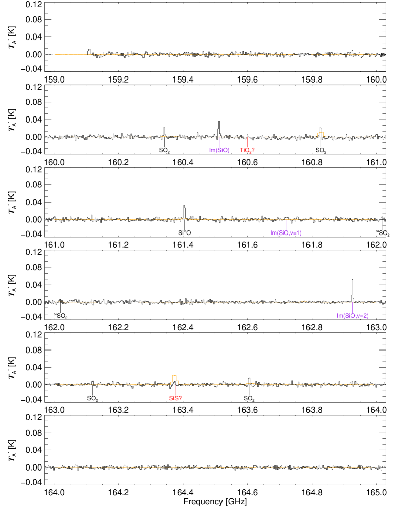
Figure 25: APEX line survey of R Dor (black). Labels show the carrier molecule of the indicated emission. Red labels indicate tentative or unidentified detections. Purple labels (Im(…)) pertain to emission contaminating the signal from the image sideband (see Sect. 2). For visibility, some parts of the survey were rescaled to fit the vertical scale. The colour coding of the spectrum corresponds to the following scale factors: (black) 1; (green) 1/5; (blue) 1/25; (red) 1/125. Note the gap in the range $321.5-328.0$ GHz. We also show the IRAM 30 m survey of IK Tau (orange; Velilla Prieto et al. 2017) for direct comparison of the two data sets. The IK Tau spectrum has been scaled according to the description in App. C.

Fig. 25. Continued.