Accelerating $N$-body simulation of self-gravitating systems with limited first-order post-Newtonian approximation

Abstract

In this study, an $N$-body simulation code was developed for self-gravitating systems with a limited first-order post-Newtonian approximation. The code was applied to a special case in which the system consists of one massive object and many low-mass objects. Therefore, the behavior of stars around the massive black hole could be analyzed. A graphics processing unit (GPU) was used to accelerate the code execution, and it could be accelerated by several tens of times compared to a single-core CPU for $N\simeq 10^{4}$ objects.

65Y05, 65Y10, 68U20, 83C10

1 Introduction

The formation of massive black holes is one of the most important problems in astrophysics. It was recently reported that a supermassive black hole (SMBH) exists at the center of the Milky Way  [1, 2]. It has also been proposed that SMBHs, whose masses are estimated to be in the range of $10^{6}-10^{10}M_{\odot}$, can exist in other galaxies, according to the relation between the SMBH mass and the luminosity [3], or the SMBH mass and bulge mass [4]. In dwarf elliptical galaxies, the relation between massive black holes and nuclear stars has been discussed [5].

For globular clusters, the existence of massive black holes remains unclear. For example, observations have indicated that the globular cluster NGC-224-G1 (or Mayall II) orbiting M31 can possess a massive black hole [6, 7]. In another case, the existence of a massive black hole in M15 (or NGC 7078) has also been discussed [8, 9]. However, definitive conclusions have not yet been reached.

Although several scenarios for the formation of SMBHs have been discussed [10], the exact scenario remains to be clearly identified. For example, if the seeds of SMBHs were stellar-mass black holes, there would be an insufficient amount of time for them to grow into such a massive black hole. The scenario where galaxies and SMBHs evolve together has also been discussed  [11].

Gravity mainly affects the formation and evolution of astronomical objects. Regarding dynamical evolution, $N$-body simulations have always been performed. When we can see the effects of radiation or pressure of baryonic gas, we must consider the hydrodynamical evolution. In contrast, we consider only the gravitational interaction between objects where we can apply $N$-body simulations, in which the interactions are described by Newtonian gravity.

However, it is inadequate to describe the interaction of objects in neighboring regions of SMBHs by Newtonian gravity alone. In Newtonian gravity, Bahcall and Wolf demonstrated that when a globular cluster possesses a massive black hole, the density distribution peaks at the center of the cluster [12]. Although their work is quite important, when we discuss the behavior of stars near a massive black hole, the effect of general relativity becomes important. Therefore, we should consider the effect of general relativity in the neighboring regions of SMBHs. For the $N$-body simulation, a post-Newtonian (PN) approach was proposed. The interaction of massive objects is extended by $(v/c)^{n}$ terms. Then, the lowest-order term ($(v/c)^{2}$) is added to the Newtonian interaction. This equation of motion for $N$-body systems is known as the EIH equation [13, 14]. The equations of motion for $N$-body systems up to the second-order PN ($(v/c)^{4}$) have also been derived  [15].

In this study, a numerical simulation code for PN $N$-body simulations was developed. Here, we note a special case, i.e., we suppose one SMBH and many stars. The interaction between the SMBH and stars are estimated by the PN approximation. Then, the interaction between stars is calculated by Newtonian gravity. In this case, the procedure of the computation is reduced. The interactions are computed on a graphics processing unit (GPU), which can process a large number of operations in parallel. Because the computation of complicated interactions is carried out on a GPU, the total computation time can be reduced.

The paper is organized as follows. In Section 2, the equation of motion and conserved quantities are described. In a generic case, because of the emission of gravitational waves, the total energy of the system decreases. In the first-order PN (1PN) approximation, because gravitational waves are not emitted, the total energy is conserved. Here, we note a special case, i.e., the system consists of one massive object and many low-mass stars. In Section 3, the numerical simulation is described. Using a GPU, the simulation can be accelerated. The elapsed time of the simulations are compared between cases of a central processing unit (CPU) only and a CPU+GPU. In Section 4, the time evolution for simple models is presented and the accuracy of the simulation is validated. Then, the time evolution between Newtonian and PN cases is compared. In Section 5, the conclusions of this study are presented.

2 Equations of motion and conserved quantities

The equations of motion for $N$-body particles with the 1PN approximation were derived nearly 100 years ago [13, 14]. These equations include the three-body interaction. Therefore, when we consider $N$ particles, the order of computation for the interaction becomes $O(N^{3})$. Because the computation of the interaction is computationally demanding, the numerical simulation appears to be quite difficult.

Here, we assume that one object is considerably heavier than the other objects. Under this assumption, the massive object only affects the relativistic correction. In other words, we consider the interaction between the massive object and other objects up to a 1PN approximation. The interaction between the other objects are described only by Newtonian gravity. By this assumption, the order of computation for the interaction decreases to $O(N^{2})$ [16].

Here, we label the massive object #$1$. Then, the mass of particle #$1$ is defined as $M$. The subscripts of the other objects are $i,j,k$. The equation of motion for the massive object can be described as follows.

$$\bm{a}_{1}=-\sum_{j}\frac{Gm_{j}\bm{x}_{1j}}{r_{1j}^{3}}+\frac{1}{c^{2}}\left[\bm{a}_{1}\right]_{BH}+\frac{1}{c^{2}}\left[\bm{a}_{1}\right]_{Cross}+O\left(\frac{G^{2}m_{j}^{3}}{Mc^{2}r^{3}}\right)\,,$$ (1)

where $m_{j}$ is the mass of object #$j$ and $\bm{x}_{1j}\equiv\bm{x}_{j}-\bm{x}_{1},r_{1j}\equiv|\bm{x}_{1j}|$. The sum over $j$ excludes #$1$. The first term of the right-hand side of Eq. (1) represents Newtonian gravity. The PN terms in Eq. (1) can be described as follows.

$$\left[\bm{a}_{1}\right]_{BH} = \sum_{j}\frac{Gm_{j}\bm{x}_{1j}}{r_{1j}^{3}}\left(5\frac{GM}{r_{1j}}-2v_{j}^{2}+\frac{3}{2}\left(\bm{v}_{j}\cdot\bm{n}_{1j}\right)\right)$$ (2)

$$+3\sum_{j}\frac{Gm_{j}}{r_{1j}^{3}}(\bm{v}_{j}\cdot\bm{x}_{1j})\bm{v}_{j}\,,$$

$$\left[\bm{a}_{1}\right]_{Cross} = 4\sum_{j}\frac{G^{2}m_{j}^{2}\bm{x}_{1j}}{r_{1j}^{4}}$$ (3)

$$+\sum_{j,k}\frac{G^{2}m_{j}m_{k}\bm{x}_{1j}}{r_{1j}^{3}}\left(\frac{4}{r_{1k}}+\frac{5}{4r_{jk}}-\frac{r_{1k}^{2}}{4r_{jk}^{3}}+\frac{r_{1j}^{2}}{4r_{jk}^{3}}\right)$$

$$-\frac{7}{2}\sum_{j,k}\frac{G^{2}m_{j}m_{k}\bm{x}_{jk}}{r_{jk}^{3}r_{1j}}$$

$$-\sum_{j,k}\frac{Gm_{j}m_{k}}{Mr_{1j}^{3}}\left[4(\bm{v}_{j}\cdot\bm{v}_{k})\bm{x}_{1j}-3(\bm{v}_{j}\cdot\bm{x}_{1j})\bm{v}_{k}-4(\bm{v}_{k}\cdot\bm{x}_{1j})\bm{v}_{j}\right]\,.$$

The sum over $k$ excludes #$1$. $\bm{n}$ is the unit vector $\bm{n}_{1j}=\bm{x}_{1j}/r_{1j}$.

The equation of motion for the low-mass stars can be described as follows.

$$\bm{a}_{i}=-\frac{GM\bm{x}_{i1}}{r_{i1}^{3}}-\sum_{j}\frac{Gm_{j}\bm{x}_{ij}}{r_{ij}}+\frac{1}{c^{2}}\left[\bm{a}_{i}\right]_{BH}+\frac{1}{c^{2}}\left[\bm{a}_{i}\right]_{Cross}+O\left(\frac{G^{2}m_{j}^{2}}{c^{2}r^{3}}\right)\,,$$ (4)

where

$$\left[\bm{a}_{i}\right]_{BH} = \frac{GM\bm{x}_{i1}}{r_{i1}^{3}}\left(4\frac{GM}{r_{i1}}-v_{i}^{2}\right)+4\frac{GM}{r_{i1}^{3}}\left(\bm{v}_{i}\cdot\bm{x}_{i1}\right)\bm{v}_{a}\,,$$ (5)

$$\left[\bm{a}_{i}\right]_{Cross} = 5\frac{G^{2}m_{i}M\bm{x}_{i1}}{r_{i1}^{4}}-\frac{Gm_{i}}{r_{i1}^{3}}\left[4v_{i}^{2}\bm{x}_{i1}-7(\bm{v}_{i}\cdot\bm{x}_{i1})\bm{v}_{i}\right]$$ (6)

$$+\sum_{j}\frac{G^{2}m_{j}M\bm{x}_{i1}}{r_{i1}^{3}}\left(\frac{4}{r_{ij}}+\frac{5}{4r_{j1}}+\frac{r_{i1}^{2}}{4r_{j1}^{3}}-\frac{r_{ij}^{2}}{4r_{j1}^{3}}\right)$$

$$+\sum_{j}\frac{G^{2}m_{j}M\bm{x}_{ij}}{r_{ij}^{3}}\left(\frac{4}{r_{i1}}+\frac{5}{4r_{j1}}-\frac{r_{i1}^{2}}{4r_{j1}^{3}}+\frac{r_{ij}^{2}}{4r_{j1}^{3}}\right)$$

$$-\frac{7}{2}\sum_{j}\frac{G^{2}m_{j}M\bm{x}_{j1}}{r_{j1}^{3}}\left(\frac{1}{r_{ij}}-\frac{1}{r_{i1}}\right)$$

$$-\sum_{j}\frac{Gm_{j}}{r_{i1}^{3}}\left[4(\bm{v}_{i}\cdot\bm{v}_{j})\bm{x}_{i1}-3(\bm{v}_{j}\cdot\bm{x}_{i1})\bm{v}_{i}-4(\bm{v}_{i}\cdot\bm{x}_{i1})\bm{v}_{j}\right]$$

$$+\sum_{j}\frac{Gm_{j}\bm{x}_{ij}}{r_{ij}^{3}}\left[v_{i}^{2}-2|\bm{v}_{ij}|^{2}+\frac{3}{2}(\bm{v}_{j}\cdot\bm{n}_{ij})^{2}\right]$$

$$+\sum_{j}\frac{Gm_{j}}{r_{ij}^{3}}\left[\bm{x}_{ij}\cdot(4\bm{v}_{i}-3\bm{v}_{j})\right]\bm{v}_{ij}\,,$$

where $\bm{v}_{ij}\equiv\bm{v}_{j}-\bm{v}_{i}$.

The total energy and $3$-momentum in the 1PN order are conserved. In the present study, we evaluate the total energy during the time evolution.

$$E = \frac{1}{2}Mv_{1}^{2}+\frac{1}{2}\sum_{i}m_{i}v_{i}^{2}-\frac{1}{2}\sum_{i,j}\frac{Gm_{i}m_{j}}{r_{ij}}-\sum_{i}\frac{GMm_{i}}{r_{1i}}$$ (7)

$$+\frac{1}{c^{2}}\left\{\frac{3}{8}\sum_{i}m_{i}v_{i}^{4}+\frac{3}{2}\sum_{i}\frac{GMm_{i}}{r_{1i}}v_{i}^{2}+\frac{1}{2}\sum_{i}\frac{G^{2}M^{2}m_{i}}{r_{1i}^{2}}\right.$$

$$~{}~{}~{}~{}+\frac{1}{4}\sum_{i,j}\frac{Gm_{i}m_{j}}{r_{ij}}\left[6v_{i}^{2}-7\bm{v}_{i}\cdot\bm{v}_{j}-(\bm{n}_{ij}\cdot\bm{v}_{i})(\bm{n}_{ij}\cdot\bm{v}_{j})\right]$$

$$~{}~{}~{}~{}+\frac{1}{2}\sum_{i}\frac{GMm_{i}}{r_{1i}}\left[3v_{1}^{2}-7\bm{v}_{1}\cdot\bm{v}_{i}-(\bm{n}_{1i}\cdot\bm{v}_{1})(\bm{n}_{1i}\cdot\bm{v}_{i})\right]$$

$$~{}~{}~{}~{}\left.+\sum_{i,j}\frac{G^{2}Mm_{i}m_{j}}{r_{ij}r_{1i}}+\frac{1}{2}\sum_{i,j}\frac{G^{2}Mm_{i}m_{j}}{r_{1i}r_{1j}}\right\}+O\left(\frac{G^{2}m_{i}^{3}}{r^{2}}\right)\,,$$

$$\bm{P} = M\bm{v}_{1}+\sum_{i}m_{i}\bm{v}_{i}\left(1+\frac{1}{2c^{2}}v_{i}^{2}\right)-\frac{1}{2c^{2}}\left\{\sum_{i}\frac{GMm_{i}}{r_{1i}}\left[\bm{v}_{i}+(\bm{v}_{i}\cdot\bm{n}_{1i})\bm{n}_{1i}\right]\right.$$ (8)

$$\left.+\sum_{i}\frac{GMm_{i}}{r_{1i}}[\bm{v}_{1}+(\bm{v}_{1}\cdot\bm{n}_{1i})\bm{n}_{1i}]+\sum_{i,j}\frac{Gm_{i}m_{j}}{r_{ij}}[\bm{v}_{i}+(\bm{v}_{i}\cdot\bm{n}_{ij})\bm{n}_{ij}]\right\}$$

$$+O\left(\frac{Gm_{i}^{3}v_{i}}{c^{2}Mr}\right)\,.$$

3 Numerical Simulation

3.1 Implementation for GPU

For the acceleration of the numerical simulation, a GPU is used for heavy calculations. For self-gravitating systems, the GRAvity piPE (GRAPE) system was developed [17]. The GRAPE processor calculates the acceleration and gravitational potential for each particle from the position and mass of particles. In the case of $N$ particles, the calculation of the acceleration and potential becomes $O(N^{2})$. Unfortunately, the GRAPE system can only be applied for Newtonian gravity. In contrast, because the GPU is programmable, we can perform a generic computation using the GPU.

Computing platforms for the development of the GPU computation have been produced, e.g., NVIDIA CUDA [18] and OpenCL [19]. Although these environments are required to describe the data transfer between the main memory and memory beside GPU, it is difficult to describe the optimized code. Instead of these environments, a command is introduced for the computation on the GPU to the source code. Here, we have applied the domain-specific compiler “Goose,” which was developed by K & F Computing Research [20]. The target loops to compute are specified on the GPU by the command. The syntax of the commands on “Goose” is similar to OpenACC [21]. Although “Goose” can be applied up to double loops, this compiler can implement the reduction command for array variables (for example, $\left[\bm{a}_{i}\right]_{BH}$) implicitly. Therefore, the computation of the acceleration can be accelerated easily. In terms of three-body interactions, the loops of the variables $j$ and $k$ expand to a significant number of threads and are executed on the GPU simultaneously.

For acceleration, we should choose the terms where the computation is significantly heavier than the input or output data transfer. In other words, when the procedure of the computation and data transfer are $O(N^{2})$ and $O(N)$, respectively, it is easy to use the GPU to accelerate it. In our case, we calculate the terms of the sum over $j,k$ in Eq. (3) and the terms of the sum over $j$ in Eqs. (4) and (6) on the GPU. Then, to evaluate the accuracy, the total energy is obtained by calculating the terms of the sum over $i,j$ in Eq. (7).

3.2 Evaluation of acceleration

For the evaluation of acceleration, the numerical code is executed on a generic PC with a GPU. The specifications of the PC are summarized in Table 3.1.

Table 3.1  Specifications of PC.
Instrument model/version/quantity CPU Intel Core i7-3770K RAM 32 GB OS CentOS 6.9 kernel Version 2.6.32-642.11.1 gcc Version 4.4.7 GPU NVIDIA Tesla K20c NVIDIA CUDA Version 4.2 Goose Version 1.3.3

Here, the number of particles $N$ are varied in the range of $[100,30000]$ and the elapsed time is measured. Table 3.2 and Figure 1 show the dependency of the number of particles for the total elapsed time. We calculate 32 time steps of time evolution with the fourth-order Runge–Kutta method [22], then calculate the total energy at both the start and end of the computation.

Table 3.2  Dependency of the number of particles for the total elapsed time. Here, we take the average of 10 samples for each case.
#$N$ $t_{GPU}$ [s] $\sigma_{t_{GPU}}$ [s] $t_{CPU}$ [s] $\sigma_{t_{CPU}}$ [s] $100$ $1.5392$ $0.1299$ $0.3479$ $0.0043$ $300$ $1.9651$ $0.1308$ $3.0501$ $0.0060$ $1000$ $1.941$ $0.1222$ $33.652$ $0.0881$ $3000$ $5.0517$ $0.1284$ $302.31$ $0.10062$ $10000$ $38.934$ $0.0100$ $3358.6$ $2.1313$ $30000$ $339.956$ $0.1391$ $30188$ $17.482$

In the case of computation on the host CPU only, the elapsed time is almost proportional to $O(N^{2})$. In contrast, in the case of computation with the GPU, because multiple threads are used, the increase in computation time is suppressed. However, when $N$ increases to $10^{4}$, the loops of the three-body interactions expand to $O(10^{8})$ threads. Therefore, the threads of the GPU seem saturated.

Figure 1: Dependency of the number of the particles on the computation time. Because the dispersion is quite small, we do not plot error bars. In the case of the host CPU only, the computation time appears to be proportional to $N^{2}$. In contrast, the computation time is suppressed by the computation on the GPU by a large number of threads. When $N$ increases to $10^{4}$, the computation time increases because the threads of the GPU become saturated.

4 Time evolution of test model

In a previous study, we analyzed the effect of a central massive object on low-mass stars with Newtonian gravity [23, 24]. In the collisionless case, an explicit symplectic integrator conserves the total energy for a significant length of time in Newtonian self-gravitational systems [25, 26, 27]. In contrast, although we can describe the Hamiltonian for this model, we cannot apply the explicit symplectic integrator, because the Hamiltonian cannot be divided into coordinate terms and momentum terms in the 1PN equations. Therefore, we apply an alternative integrator. The terms of the 1PN appear to be complicated; therefore, we avoid computing the time derivative of these terms.

In this study, we apply the fourth-order Runge–Kutta integration method. Unlike the symplectic integrator, the Runge–Kutta method does not conserve the total energy in the global timescale.

In the simulation, we set the constant $c=G=1$. Then, the total mass of low-mass stars is set as

$$\sum_{i\neq 1}m_{i}=1\,.$$ (9)

In this case, the Schwarzschild radius of the massive object becomes $2GM/c^{2}=2M$. We expect that the effect of general relativity appears only around the Schwarzschild radius of the massive object.

The initial condition of the test model is given by a spherically symmetric distribution. The low-mass stars are distributed in the region for $1<r<10$. The spatial distribution is generated by a random number from linear congruential generators [22]. The total number of low-mass stars is $N=10000$. Then, we assume that all the low-mass stars have equal mass. In other words, the mass of the low-mass stars is given by $m=1/N=10^{-4}$. Then, the massive object $M=100m$ is set at the origin. The Schwarzschild radius of the massive object becomes $R_{Sch}=0.02$. The initial velocity of both the massive object and low-mass stars is set to zero. In other words, we suppose a cold collapse of the system.

To avoid the dispersion of the interaction at the collision, we introduce Plummer softening to the inverse of the distance between stars.

$$\frac{1}{r}\rightarrow\frac{1}{\sqrt{r^{2}+\varepsilon^{2}}}\,.$$ (10)

In this study, we set the softening parameter $\varepsilon=10^{-3}$, which is shorter than the Schwarzschild radius of the massive object.

The time step is set as $\Delta t=2^{-17}$. Here, we calculate the time evolution until $t=10$. The error of the total energy reaches up to the 1PN order (Eq. (7)), as shown in Figure 2. Although the total energy of the system is conserved, because the Runge–Kutta method includes the global error, the error of the total energy increases during the time evolution. When we change the time step ($\Delta t=2^{-16},2^{-15}$), the error of the total energy is nearly unchanged. At $t=10$, the error of the total energy increases to about $10^{-2}$. The origin of the energy error can be considered as the accumulated error because of the long time integration.

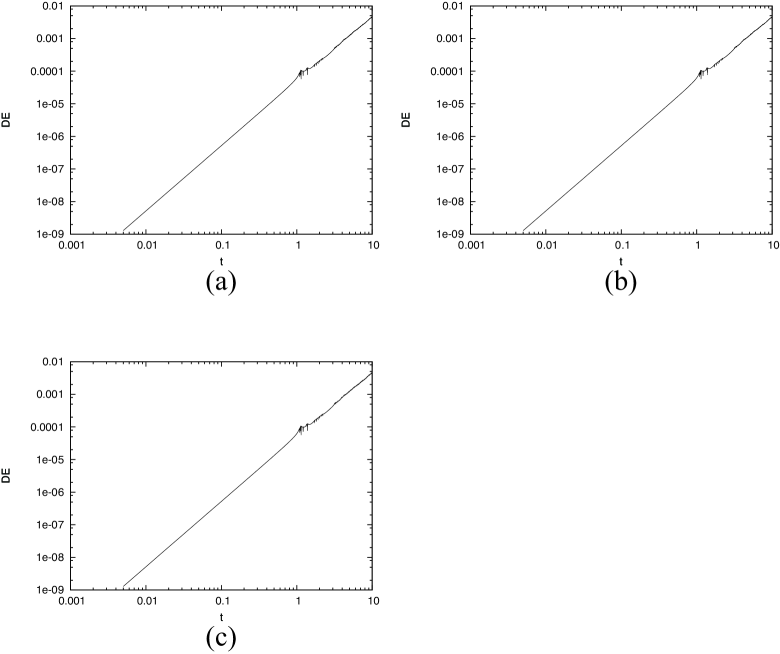
Figure 2: Error of the total energy during time evolution. (a) $\Delta t=2^{-17}$, (b) $\Delta t=2^{-16}$, and (c) $\Delta t=2^{-15}$.

For analysis of the long duration, we simulate the system with $\Delta t=2^{-15}$ until $t=100$. As is the global tendency, the stars fall to the center. During evolution, the low-mass stars form binary systems of local clusters. Figure 3 shows the distance of the nearest low-mass binary stars. The low-mass stars scatter at $t\simeq 1$. According to the effect of the scattering by low-mass stars and the formation of binaries, the error of the total energy can oscillate. Figure 4 shows the distance between the massive object and nearest low-mass star. At $t\simeq 17$, one low-mass star is scattered by the massive object. Then, the error of the total energy increases abruptly (Fig. 5). Because the simulation fails at the scattering of low-mass stars around the massive object, we should use a more accurate integrator such as the Hermite scheme for the time evolution in collisional systems.

Figure 3: Distance of the nearest low-mass binary stars. At $t\simeq 1$, the low-mass stars collide with each other. Then, the low-mass stars form binary systems.

Figure 4: Distance between the massive object and nearest low-mass star. At $t\simeq 17$, one low-mass star approaches the massive object. Then, the low-mass star is scattered.

Figure 5: Error of total energy during the time evolution for computation time. Here, we set $\Delta t=2^{-15}$. At $t\simeq 17$, one low-mass star approaches the massive object. Then, a significant error appears in the total energy. After this scattering, the simulation fails.

5 Summary

In this study, an $N$-body simulation code was developed for a limited 1PN approximation. The simulation was accelerated by a GPU, where we could conduct realistic simulations of globular clusters with a massive object such as an intermediate-mass black hole (IMBH).

One of the critical problems in astrophysics is the conservation of total energy. Because the equation of motion in the 1PN approximation cannot be divided into spatial terms and momentum terms, an explicit symplectic integrator cannot be applied. As another method, the Hermite integrator was developed [28, 29, 30]. Although the Hermite integrator is known as a high-accuracy method, the time-derivative of the acceleration is required. Therefore, it is difficult to apply the Hermite method to the $N$-body simulation code for the 1PN approximation. The time derivative of the accelerations is described in Appendix A. Because the acceleration includes three-body interactions, the time derivative of the accelerations becomes quite complicated.

In this study, a limited 1PN approximation is considered. This code can simulate the evolution of several astronomical objects such as globular clusters with IMBHs, accretion disks around black holes, and others. For example, the code could simulate the accretion around Sgr A^∗ [31, 32].

As one of the scenarios of SMBH formation, the merging of many stellar-mass black holes has been considered. For this scenario, we developed a generic 1PN approximation code with a GPU. In the generic 1PN approximation, the cost of the computation becomes $O(N^{3})$. In a previous study, Kupi et al. proposed a direct method for time integration with the PN approximation  [33]. Then, Brem et al. implemented the spin effects and presented a step forward in higher-order terms [34]. In other studies using the regularization method for the collision of stars, the higher-order PN approximation was implemented  [35, 36, 37, 38].

We implemented the 1PN approximation for the full simulation. We consider that the critical point could be the data transfer between the GPU and main memory and the handling of shared memories In previous studies using Newtonian gravity, it has been reported that a conspicuous difference in the performances appears according to how the shared memories are handled [39, 40] Because “Goose” cannot be applied up to the triple loop, the command in “Goose” cannot reduce the data transfer to $O(N)$. The data transfer can be reduced only to $O(N^{2})$. For the handling of shared memories and reduction of the data transfer, we require detailed coding for a generic 1PN approximation using a CUDA C environment.

When we run this simulation, the formation process for SMBHs from many stellar-mass black holes can be determined. By using a GPU with a very large number of threads, the computation time is expected to reduce considerably compared to that in general-purpose computers.

Appendix A Time derivation of the acceleration

For the Hermite scheme, we require the time derivative of the acceleration for time evolution. The time derivative of the acceleration for massive objects can be described as follows:

$$\frac{\partial}{\partial t}\bm{a}_{1} = \frac{\partial}{\partial t}\left(-\sum_{j}\frac{Gm_{j}\bm{x}_{1j}}{r_{1j}^{3}}\right)+\frac{\partial}{\partial t}\left[\bm{a}_{1}\right]_{BH}+\frac{\partial}{\partial t}\left[\bm{a}_{1}\right]_{Cross}\,,$$ (11)

$$\frac{\partial}{\partial t}\left(-\sum_{j}\frac{Gm_{j}\bm{x}_{1j}}{r_{1j}^{3}}\right) = -Gm_{j}\left(\frac{\bm{v}_{1j}}{r_{1j}^{3}}-3\frac{(\bm{x}_{1j}\cdot\bm{v}_{1j})}{r_{1j}^{5}}\bm{x}_{1j}\right)\,,$$ (12)

$$\frac{\partial}{\partial t}\left[\bm{a}_{1}\right]_{BH} = \sum_{j}\frac{Gm_{j}}{r_{1j}^{3}}\left(-5\frac{GM(\bm{x}_{1j}\cdot\bm{v}_{1j})}{r_{1j}^{3}}-4(\bm{v}_{j}\cdot\bm{a}_{j})+\frac{3}{2}(\bm{a}_{j}\cdot\bm{n}_{1j})\right.$$ (13)

$$~{}~{}~{}~{}~{}~{}~{}~{}~{}~{}~{}~{}~{}~{}~{}~{}\left.-\frac{3}{2}\frac{1}{r_{1j}}(\bm{v}_{j}\cdot\bm{x}_{1j})(\bm{v}_{1j}\cdot\bm{x}_{1j})+\frac{3}{2}\frac{(\bm{v}_{j}\cdot\bm{v}_{1j})}{r_{1j}}\right)\bm{x}_{ij}$$

$$+\sum_{j}Gm_{j}\left(-\frac{3}{r_{1j}^{5}}(\bm{v}_{1j}\cdot\bm{x}_{1j})\bm{x}_{1j}+\frac{\bm{v}_{1j}}{r_{1j}^{3}}\right)\left(5\frac{GM}{r_{1j}}-2v_{j}^{2}+\frac{3}{2}(\bm{v}_{j}\cdot\bm{n}_{ij})\right)$$

$$-9\sum_{j}\frac{Gm_{j}}{r_{1j}^{6}}(\bm{v}_{1j}\cdot\bm{x}_{1j})(\bm{v}_{j}\cdot\bm{x}_{1j})\bm{v}_{j}$$

$$+3\sum_{j}\frac{Gm_{j}}{r_{1j}^{3}}\left\{(\bm{a}_{j}\cdot\bm{x}_{1j})\bm{v}_{j}+(\bm{v}_{j}\cdot\bm{v}_{1j})\bm{v}_{j}+(\bm{v}_{j}\cdot\bm{x}_{1j})\bm{a}_{j}\right\}\,,$$

$$\frac{\partial}{\partial t}\left[\bm{a}_{1}\right]_{Cross} = 4\sum_{j}G^{2}m_{j}^{2}\left(\frac{\bm{v}_{1j}}{r_{1j}^{4}}-4\frac{(\bm{x}_{1j}\cdot\bm{v}_{1j})}{r_{1j}^{6}}\bm{x}_{1j}\right)$$ (14)

$$+\sum_{j,k}G^{2}m_{j}m_{k}\left(\frac{\bm{v}_{1j}}{r_{1j}^{3}}-3\frac{(\bm{x}_{1j}\cdot\bm{v}_{1j})}{r_{1j}^{6}}\bm{x}_{1j}\right)\left(\frac{4}{r_{1k}}+\frac{5}{4r_{jk}}-\frac{r_{1k}^{2}}{4r_{jk}^{3}}+\frac{r_{1j}^{2}}{4r_{jk}^{3}}\right)$$

$$+\sum_{j,k}\frac{G^{2}m_{j}m_{k}\bm{x}_{1j}}{r_{1j}^{3}}\left(-\frac{4}{r_{1k}^{3}}(\bm{v}_{1k}\cdot\bm{x}_{1k})-\frac{5}{4r_{jk}^{3}}(\bm{x}_{jk}\cdot\bm{v}_{jk})-\frac{(\bm{x}_{1k}\cdot\bm{v}_{1k})}{2r_{jk}^{3}}\right.$$

$$~{}~{}~{}~{}~{}~{}~{}~{}~{}~{}~{}~{}~{}~{}~{}~{}\left.-\frac{3r_{1k}^{2}(\bm{x}_{jk}\cdot\bm{v}_{jk})}{4r_{jk}^{5}}+\frac{(\bm{x}_{1j}\cdot\bm{v}_{1j})}{2r_{jk}^{3}}+\frac{3r_{1j}^{2}(\bm{x}_{jk}\cdot\bm{v}_{jk})}{4r_{jk}^{5}}\right)$$

$$-\frac{7}{2}\sum_{j,k}\frac{G^{2}m_{j}m_{k}\bm{v}_{jk}}{r_{jk}^{3}r_{1j}}$$

$$+\frac{7}{2}\sum_{j,k}G^{2}m_{j}m_{k}\left(\frac{3(\bm{x}_{jk}\cdot\bm{v}_{jk})}{r_{jk}^{5}r_{1j}}+\frac{(\bm{x}_{1j}\cdot\bm{v}_{1j})}{r_{jk}^{3}r_{1j}^{3}}\right)\bm{x}_{jk}$$

$$-\sum_{j,k}\frac{Gm_{j}m_{k}}{Mr_{1j}^{3}}\left(4(\bm{a}_{j}\cdot\bm{v}_{k})\bm{x}_{1j}+4(\bm{v}_{j}\cdot\bm{a}_{k})\bm{x}_{1j}+4(\bm{v}_{j}\cdot\bm{v}_{k})\bm{v}_{1j}\right.$$

$$~{}~{}~{}~{}~{}~{}~{}~{}~{}~{}~{}~{}~{}~{}~{}~{}-3(\bm{a}_{j}\cdot\bm{x}_{1j})\bm{v}_{k}-3(\bm{v}_{j}\cdot\bm{v}_{1j})\bm{v}_{k}-3(\bm{v}_{j}\cdot\bm{x}_{1k})\bm{a}_{k}$$

$$~{}~{}~{}~{}~{}~{}~{}~{}~{}~{}~{}~{}~{}~{}~{}~{}\left.-4(\bm{a}_{k}\cdot\bm{x}_{1j})\bm{v}_{k}-4(\bm{v}_{k}\cdot\bm{v}_{1j})\bm{v}_{k}-4(\bm{v}_{k}\cdot\bm{x}_{1j})\bm{a}_{k}\right)\,.$$

The time derivative of the acceleration for low-mass stars can be described as follows:

$$\frac{\partial}{\partial t}\bm{a}_{i} = \frac{\partial}{\partial t}\left(-\frac{GM\bm{x}_{j1}}{r_{j1}^{3}}-\sum_{j}\frac{Gm_{j}\bm{x}_{ij}}{r_{ij}^{3}}\right)+\frac{\partial}{\partial t}\left[\bm{a}_{i}\right]_{BH}+\frac{\partial}{\partial t}\left[\bm{a}_{i}\right]_{Cross}\,,$$ (15)

$$\frac{\partial}{\partial t}\left(-\frac{GM\bm{x}_{j1}}{r_{j1}^{3}}-\sum_{j}\frac{Gm_{j}\bm{x}_{ij}}{r_{ij}^{3}}\right) = -GM\left(\frac{\bm{v}_{j1}}{r_{j1}^{3}}-3\frac{(\bm{x}_{j1}\cdot\bm{v}_{j1})}{r_{j1}^{5}}\bm{x}_{j1}\right)$$ (16)

$$-Gm_{j}\left(\frac{\bm{v}_{ij}}{r_{ij}^{3}}-3\frac{(\bm{x}_{ij}\cdot\bm{v}_{ij})}{r_{ij}^{5}}\bm{x}_{ij}\right)\,,$$

$$\frac{\partial}{\partial t}\left[\bm{a}_{i}\right]_{BH} = \frac{4G^{2}M^{2}}{r_{i1}^{6}}\left(r_{i1}^{2}\bm{v}_{i1}-4(\bm{x}_{i1}\cdot\bm{v}_{i1})\bm{x}_{i1}\right)$$ (17)

$$-\frac{GM}{r_{i1}^{3}}v_{i}^{2}\bm{v}_{i1}-\frac{2GM}{r_{i1}^{3}}(\bm{v}_{i}\cdot\bm{a}_{i})\bm{x}_{i1}+\frac{3GM}{r_{i1}^{5}}v_{i}^{2}(\bm{x}_{i1}\cdot\bm{v}_{i1})\bm{x}_{i1}\,,$$

$$\frac{\partial}{\partial t}\left[\bm{a}_{i}\right]_{Cross} = 5\frac{G^{2}m_{i}M\bm{v}_{i1}}{r_{i1}^{4}}-20\frac{G^{2}m_{i}M(\bm{x}_{i1}\cdot\bm{v}_{i1})}{r_{i1}^{6}}\bm{x}_{i1}$$

$$-3\frac{Gm_{i}(\bm{x}_{i1}\cdot\bm{v}_{i1})}{r_{i1}^{5}}\left(4v_{i}^{2}\bm{x}_{i1}-7(\bm{v}_{i}\cdot\bm{x}_{i1})\bm{v}_{i}\right)$$

$$-\frac{Gm_{i}}{r_{i1}^{3}}\left[8(\bm{v}_{i}\cdot\bm{a}_{i})\bm{x}_{i1}+4v_{i}^{2}\bm{v}_{i1}-7\left((\bm{a}_{i}\cdot\bm{x}_{i1})+(\bm{v}_{i}\cdot\bm{v}_{i1})\right)\bm{v}_{i}\right.$$

$$~{}~{}~{}~{}~{}~{}~{}~{}\left.-7(\bm{v}_{i}\cdot\bm{x}_{i1})\bm{a}_{i}\right]$$

$$+\sum_{j}\frac{G^{2}m_{j}M\bm{v}_{i1}}{r_{i1}^{3}}\left(\frac{4}{r_{ij}}+\frac{5}{4r_{j1}}+\frac{r_{i1}^{2}}{4r_{ji}^{3}}-\frac{r_{ij}^{2}}{4r_{j1}^{3}}\right)$$

$$-3\sum_{j}\frac{G^{2}m_{j}M(\bm{x}_{i1}\cdot\bm{v}_{i1})\bm{v}_{i1}}{r_{i1}^{5}}\left(\frac{4}{r_{ij}}+\frac{5}{4r_{j1}}+\frac{r_{i1}^{2}}{4r_{ji}^{3}}-\frac{r_{ij}^{2}}{4r_{j1}^{3}}\right)$$

$$+\sum_{j}\frac{G^{2}m_{j}M\bm{x}_{i1}}{r_{i1}^{3}}\left(-\frac{4(\bm{x}_{ij}\cdot\bm{v}_{ij})}{r_{ij}^{3}}-\frac{5(\bm{x}_{j1}\cdot\bm{v}_{j1})}{4r_{j1}^{3}}+\frac{(\bm{x}_{i1}\cdot\bm{v}_{i1})}{2r_{j1}^{3}}\right.$$

$$~{}~{}~{}~{}~{}~{}~{}~{}~{}~{}~{}~{}\left.-\frac{3(\bm{x}_{j1}\cdot\bm{v}_{j1})r_{i1}^{2}}{4r_{j1}^{5}}-\frac{(\bm{x}_{ij}\cdot\bm{v}_{ij})}{2r_{j1}^{3}}+\frac{3(\bm{x}_{j1}\cdot\bm{v}_{j1})r_{ij}^{2}}{4r_{j1}^{5}}\right)$$

$$+\sum_{j}\frac{G^{2}m_{j}M\bm{v}_{ij}}{r_{ij}^{3}}\left(\frac{4}{r_{ij}}+\frac{5}{4r_{j1}}+\frac{r_{i1}^{2}}{4r_{ji}^{3}}-\frac{r_{ij}^{2}}{4r_{j1}^{3}}\right)$$

$$-3\sum_{j}\frac{G^{2}m_{j}M(\bm{x}_{ij}\cdot\bm{v}_{ij})\bm{v}_{ij}}{r_{ij}^{5}}\left(\frac{4}{r_{ij}}+\frac{5}{4r_{j1}}+\frac{r_{i1}^{2}}{4r_{ji}^{3}}-\frac{r_{ij}^{2}}{4r_{j1}^{3}}\right)$$

$$+\sum_{j}\frac{G^{2}m_{j}M\bm{x}_{ij}}{r_{ij}^{3}}\left(-\frac{4(\bm{x}_{i1}\cdot\bm{v}_{i1})}{r_{i1}^{3}}-\frac{5(\bm{x}_{j1}\cdot\bm{v}_{j1})}{4r_{j1}^{3}}-\frac{(\bm{x}_{i1}\cdot\bm{v}_{i1})}{2r_{j1}^{3}}\right.$$

$$~{}~{}~{}~{}~{}~{}~{}~{}~{}~{}~{}~{}~{}\left.+\frac{3(\bm{x}_{j1}\cdot\bm{v}_{j1})r_{i1}^{2}}{4r_{j1}^{3}}+\frac{(\bm{x}_{ij}\cdot\bm{v}_{ij})}{2r_{j1}^{3}}-\frac{3(\bm{x}_{j1}\cdot\bm{v}_{j1})r_{ij}^{2}}{4r_{j1}^{5}}\right)$$

$$-\frac{7}{2}\sum_{j}G^{2}m_{j}M\left(\frac{\bm{v}_{j1}}{r_{j1}^{3}}-\frac{3(\bm{x}_{j1}\cdot\bm{v}_{j1})}{r_{j1}^{5}}\bm{x}_{j1}\right)\left(\frac{1}{r_{ij}}-\frac{1}{r_{i1}}\right)$$

$$+\frac{7}{2}\sum_{j}\frac{G^{2}m_{j}M\bm{x}_{j1}}{r_{j1}^{3}}\left(\frac{(\bm{x}_{ij}\cdot\bm{v}_{ij})}{r_{ij}^{3}}-\frac{(\bm{x}_{i1}\cdot\bm{v}_{i1})}{r_{i1}^{3}}\right)$$

$$+\sum_{j}\frac{Gm_{j}}{r_{i1}^{5}}(\bm{r}_{i1}\cdot\bm{v}_{i1})\left[4(\bm{v}_{i}\cdot\bm{v}_{j})\bm{x}_{i1}-3(\bm{v}_{j}\cdot\bm{x}_{i1})\bm{v}_{i}-4(\bm{v}_{i}\cdot\bm{x}_{i1})\bm{v}_{j}\right]$$

$$-\sum_{j}\frac{Gm_{j}}{r_{i1}^{3}}\left[4(\bm{a}_{i}\cdot\bm{v}_{j})\bm{x}_{i1}+4(\bm{v}_{i}\cdot\bm{a}_{j})\bm{x}_{i1}+4(\bm{v}_{i}\cdot\bm{v}_{j})\bm{v}_{i1}\right.$$

$$~{}~{}~{}~{}~{}~{}~{}~{}-3(\bm{a}_{j}\cdot\bm{x}_{i1})\bm{v}_{i}-3(\bm{v}_{j}\cdot\bm{v}_{i1})\bm{v}_{i}-3(\bm{v}_{j}\cdot\bm{x}_{i1})\bm{a}_{i}$$

$$~{}~{}~{}~{}~{}~{}~{}~{}\left.-4(\bm{a}_{i}\cdot\bm{x}_{i1})\bm{v}_{j}-4(\bm{v}_{i}\cdot\bm{v}_{i1})\bm{v}_{j}-4(\bm{v}_{i}\cdot\bm{x}_{i1})\bm{a}_{j}\right]$$

$$+\sum_{j}\frac{Gm_{j}\bm{v}_{ij}}{r_{ij}^{3}}\left[v_{i}^{2}-2|\bm{v}_{ij}|^{2}+\frac{3}{2}(\bm{v}_{j}\cdot\bm{n}_{ij})^{2}\right]$$

$$-\sum_{j}\frac{3Gm_{j}(\bm{x}_{ij}\cdot\bm{v}_{ij})\bm{x}_{ij}}{r_{ij}^{5}}\left[v_{i}^{2}-2|\bm{v}_{ij}|^{2}+\frac{3}{2}(\bm{v}_{j}\cdot\bm{n}_{ij})^{2}\right]$$

$$+\sum_{j}\frac{2Gm_{j}\bm{x}_{ij}}{r_{ij}^{3}}\left((\bm{v}_{i}\cdot\bm{a}_{i})-2(\bm{v}_{ij}\cdot\bm{a}_{ij})\right)$$

$$+\sum_{j}\frac{3Gm_{j}\bm{v}_{ij}}{2r_{ij}^{5}}(\bm{v}_{j}\cdot\bm{x}_{ij})^{2}-\frac{15Gm_{j}(\bm{x}_{ij}\cdot\bm{v}_{ij})\bm{x}_{ij}}{r_{ij}^{7}}(\bm{v}_{j}\cdot\bm{x}_{ij})^{2}$$

$$+\sum_{j}\frac{3Gm_{j}\bm{x}_{ij}}{r_{ij}^{5}}\left[(\bm{a}_{j}\cdot\bm{x}_{ij})+(\bm{v}_{j}\cdot\bm{v}_{ij})\right](\bm{v}_{j}\cdot\bm{x}_{ij})$$

$$-\sum_{j}\frac{3Gm_{j}(\bm{x}_{ij}\cdot\bm{v}_{ij})}{r_{ij}^{5}}\left[\bm{x}_{ij}\cdot(4\bm{v}_{i}-3\bm{v}_{j})\right]\bm{v}_{ij}$$

$$+\sum_{j}\frac{Gm_{j}}{r_{ij}^{3}}\left[\left\{\bm{v}_{ij}\cdot(4\bm{v}_{i}-3\bm{v}_{j})\right\}+\left\{\bm{x}_{ij}\cdot(4\bm{a}_{i}-3\bm{a}_{j})\right\}\right]\bm{v}_{ij}$$

$$+\sum_{j}\frac{Gm_{j}}{r_{ij}^{3}}\left[\bm{x}_{ij}\cdot(4\bm{v}_{i}-3\bm{v}_{j})\right]\bm{a}_{ij}\,.$$ (18)

In these equations, the acceleration $\bm{a}_{1},\bm{a}_{i}$ has already been described in Eqs. (1) and (4).

References

- [1] R. Schödel et al., A star in a 15.2-year orbit around the supermassive black hole at the centre of the Milky Way, Nature, 419 (2002) 694.
- [2] S. Gillessen et al., Monitoring Stellar Orbits around the Massive Black Hole in the Galacticx Center, Astrophys. J., 692 (2009) 1075.
- [3] A. Marconi and L. K. Hunt, The Relation between Black Hole Mass, Bulge Mass, and Near-Infrared Luminosity, Astrophys. J., 589 (2003) L21.
- [4] N. Häring and H.-W. Rix, On the Black Hole Mass-Bulge Mass Relation, Astrophys. J., 604 (2004) L89.
- [5] A. W. Graham and L. R. Spitler, Quantifying the coexistence of massive black holes and dense nuclear star clusters, Mon. Not. R. Astron. Soc., 397 (2009) 2148.
- [6] K. Gebhardt, R. M. Rich, L. C. Ho, A 20,000 Black Hole in the Stellar Cluster G1, Astrophys. J., 578 (2002) L41.
- [7] K. Gebhardt, R. M. Rich, L. C. Ho, An Intermediate-Mass Black Hole in the Globular Cluster G1: Improved Significance from New Keck and Hubble Space Telescope Observations, Astrophys. J., 634 (2005) 1093.
- [8] J. Gerssen et al., Hubble Space Telescope Evidence for an Intermediate-Mass Black Hole in the Globular Cluster M15. II. Kinematic Analysis and Dynamical Modeling, Astron. J., 124 (2002) 3270.
- [9] H. Baumgardt et al., On the Central Structure of M15, Astrophys. J., 582 (2003) L21.
- [10] M. J. Rees, Black Hole Models for Active Galactic Nuclei, Ann. Rev. Astron. Astrophys., 22 (1984) 471.
- [11] J. Kormendy and L. C. Ho, Coevolution (Or Not) of Supermassive Black Holes and Host Galaxies, Ann. Rev. Astron. Astrophys., 51 (2013) 511.
- [12] J. N. Bahcall and R. A. Wolf, Star distribution around a massive black hole in a globular cluster, Astrophys. J., 209 (1976) 214.
- [13] H. A. Lorentz and J. Droste, The motion of a system of bodies under the influence of their mutual attraction, according to Einstein’s theory, in The Collected Papers of H.A. Lorentz, Vol. 5, pp. 330-355, Nijhoff, The Hague, 1937.
- [14] A. Einstein, L. Infeld, and B. Hoffmann, The gravitational equations and the problem of motion, Ann. Math., 39 (1938) 65.
- [15] T. Ohta, H. Okamura, T.. Kimura,, K. Hiida , Physically Acceptable Solution of Einstein?s Equation for Many-Body System, Prog. Theor. Phys., 50, 492.
- [16] C. M. Will, Incorporating post-Newtonian effects in -body dynamics, Phys. Rev. D, 89 (2014) 044043.
- [17] D. Sugimoto et al., A special-purpose computer for gravitational many-body problems, Nature, 345 (1990) 33.
-
[18]
NVIDIA CUDA Parallel Computing Platform
http://www.nvidia.com/object/cuda_home_new.html -
[19]
OpenCL
https://www.khronos.org/opencl/ -
[20]
Goose compiler (K & F Computing Research)
http://www.kfcr.jp/goose-e.html -
[21]
OpenACC
http://www.openacc.org/ - [22] W. H. Press, S. A. Teukolsky, W. T. Vetterling, B. P. Flannery, Numerical Recipes in C, Cambridge Univ. Press., Cambridge, 1982.
- [23] T. Tashiro and T. Tatekawa, Brownian dynamics around the core of self-gravitating systems, J. Phys. Soc. Jpn., 79 (2010) 063001.
- [24] T. Tashiro and T. Tatekawa, Stochastic Dynamics Toward the Steady State of Self-Gravitating Systems, Numerical Simulations of Physical and Engineering Processes, pp. 301-318, Jan Awrejcewicz (Ed.), INTECH, Croatia, 2011.
- [25] M. Suzuki, General theory of higher-order decomposition of exponential operators and symplectic integrators, Phys. Lett. A, 165 (1992) 387.
- [26] H. Yoshida, Construction of higher order symplectic integrators, Phys. Lett. A, 150 (1990) 262.
- [27] H. Yoshida, Recent progress in the theory and application of symplectic integrators, Celes. Mech. Dyn. Astron., 56 (1993) 27.
- [28] J. Makino, Optimal order and time-step criterion for Aarseth-type N-body integrators Astrophys. J., 369 (1991) 200.
- [29] J. Makino and S. J. Aarseth, On a Hermite integrator with Ahmad-Cohen scheme for gravitational many-body problems Pub. Astron. Soc. Jpn., 44 (1992) 141
- [30] K. Nitadori and J. Makino, Sixth-and eighth-order Hermite integrator for N-body simulations, New Astron., 13 (2008) 498.
- [31] S. Gillessen et al., A gas cloud on its way towards the supermassive black hole at the Galactic Centre, Nature, 481 (2012) 51.
- [32] G. Ponti et al., Fifteen years of XMM-Newton and Chandra monitoring of Sgr A∗: evidence for a recent increase in the bright flaring rate, Mon. Not. R. Astron. Soc., 454 (2015) 1525.
- [33] G. Kupi, P. Amaro-Seoane, R. Spurzem, Dynamics of compact object clusters: a post-Newtonian study, Mon. Not. R. Astron. Soc., 371 (2006) L45.
- [34] P. Brem, P. Amaro-Seoane, C. F. Sopuerta, Blocking low-eccentricity EMRIs: a statistical direct-summation -body study of the Schwarzschild barrier, Mon. Not. R. Astron. Soc., 437 (2014) 1259.
- [35] S. J. Aarseth, Post-Newtonian N-body simulations, Mon. Not. R. Astron. Soc., 378 (2007) 285.
- [36] S. Harfst, A. Gualandris, D. Merritt, S. Mikkola, A hybrid N-body code incorporating algorithmic regularization and post-Newtonian forces, Mon. Not. R. Astron. Soc., 389 (2008) 2.
- [37] S. J. Aarseth, Mergers and ejections of black holes in globular clusters, Mon. Not. R. Astron. Soc., 422 (2012) 841.
- [38] S. J. Karl et al., Dynamical evolution of massive black holes in galactic-scale N-body simulations - introducing the regularized tree code ‘rVINE’, Mon. Not. R. Astron. Soc., 452 (2015) 2337.
- [39] S. F. Portegies Zwart, R. G. Belleman, P. G. Geldof, High Performance Direct Gravitational N-body Simulations on Graphics Processing Unit I: An implementation in Cg, New Astron. 12 (2007) 641.
- [40] T. Hamada and T. Iitaka, The Chamomile Scheme: An Optimized Algorithm for N-body simulations on Programmable Graphics Processing Units, arXiv:astro-ph/0703100.