The Conditional Colour-Magnitude Distribution: I. A Comprehensive Model of the Colour-Magnitude-Halo Mass Distribution of Present-Day Galaxies

Abstract

We formulate a model of the conditional colour-magnitude distribution (CCMD) to describe the distribution of galaxy luminosity and colour as a function of halo mass. It consists of two populations of different colour distributions, dubbed pseudo-blue and pseudo-red, respectively, with each further separated into central and satellite galaxies. We define a global parameterization of these four colour-magnitude distributions and their dependence on halo mass, and we infer parameter values by simultaneously fitting the space densities and auto-correlation functions of 79 galaxy samples from the Sloan Digital Sky Survey defined by fine bins in the colour-magnitude diagram (CMD). The model deprojects the overall galaxy CMD, revealing its tomography along the halo mass direction. The bimodality of the colour distribution is driven by central galaxies at most luminosities, though at low luminosities it is driven by the difference between blue centrals and red satellites. For central galaxies, the two pseudo-colour components are distinct and orthogonal to each other in the CCMD: at fixed halo mass, pseudo-blue galaxies have a narrow luminosity range and broad colour range, while pseudo-red galaxies have a narrow colour range and broad luminosity range. For pseudo-blue centrals, luminosity correlates tightly with halo mass, while for pseudo-red galaxies colour correlates more tightly (redder galaxies in more massive haloes). The satellite fraction is higher for redder and for fainter galaxies, with colour a stronger indicator than luminosity. We discuss the implications of the results and further applications of the CCMD model.

1 Introduction

Among all the galaxy physical properties directly measurable from observation with galaxy surveys, such as luminosity, colour, surface brightness, morphology, and environment, luminosity and colour jointly are the two most predictive ones for the underlying action and cessation of star formation inside galaxies. At fixed luminosity and colour, it has been shown that there is little residual correlation between environment and surface brightness or morphology (Blanton et al., 2005b). In principle, galaxy luminosity can be regarded as a zero-th order proxy to galaxy stellar mass, while in detail it is also linked to the galaxy star formation history and the age of the stellar population. Galaxy colour is an approximate indicator of star formation activity and status, and it is also related to galaxy metallicity and dust content.

In this paper, we develop a formalism to study the luminosity and colour distribution of galaxies through galaxy clustering and apply it to galaxy survey data. The model substantially extends previous methods to connect galaxies with dark matter haloes, presenting a quantitative global description of the joint colour-magnitude distribution as a function of halo mass for galaxies in the Sloan Digital Sky Survey (SDSS; York et al. 2000) main galaxy redshift survey (Strauss et al., 2002).

In the local universe, the distribution of galaxy luminosity and colour (or the colour-magnitude diagram; CMD) shows ordered patterns (e.g. Strateva et al., 2001; Blanton et al., 2003b; Baldry et al., 2004). Towards the low luminosity part in the CMD, galaxies form a diffuse ‘blue cloud’, which mainly consists of late-type galaxies with star formation. There is also a tight ‘red sequence’ of galaxies stretching from the faint end all the way to the luminous end, which is mainly made of early-type galaxies lacking star formation. A ‘green valley’ lies in between the blue cloud and red sequence. The bimodal colour distribution of galaxies has already emerged early in the history of the universe (e.g. $z\sim$1–2.5; Faber et al. 2007; Brammer et al. 2009; Coil et al. 2017). The formation of the bimodality involves mechanisms responsible for transforming the young active blue galaxies to old passive red ones, through quenching the star formation. The quenching mechanisms can be broadly divided into ‘internal’ and ‘external’ processes. Star-formation and active galactic nuclei (AGN) feedback that heats or blows away the gas and secular process that uses up the gas slowly belong to the former. Processes that quench star formation inside high density environment belong to the latter, such as ram-pressure stripping to remove the cold gas (e.g. Gunn & Gott, 1972) and strangulation to cut off the cold gas supply (e.g. Peng et al., 2015). Faber et al. (2007) investigate the evolution of luminosity function (LF) of blue and red galaxies since $z\sim 1$ and find that there is little evolution in the number density and stellar mass of blue galaxies, while those of red galaxies have dramatically increased. A ‘mixed’ scenario is thus proposed to explain the new red galaxies in which blue star-forming galaxies are quenched by gas-rich major mergers and then move along the red sequence by a series of gas-poor mergers.

In the standard paradigm of galaxy formation and evolution (e.g. White & Rees, 1978), galaxies form and evolve inside dark matter haloes. To some degree, all the physical processes affecting a galaxy are unavoidably connected to its parent halo. Linking galaxy properties (e.g. luminosity and colour) to haloes forms an important step towards learning about the galaxy formation processes. Without resorting to numerically expensive cosmological hydrodynamic simulation or semi-analytic galaxy formation models (SAM), there are empirical approaches within the halo model to establish the relation between galaxy luminosity and colour and dark matter haloes. One approach is to construct galaxy group catalogues (e.g. Yang et al., 2005a; Berlind et al., 2006; Yang et al., 2007), with each group representing a dark matter halo. Using a galaxy group catalogue, Yang et al. (2008) study the conditional luminosity functions (CLFs) of red and blue galaxies and van den Bosch et al. (2008) investigate the satellite properties. When interpreting the results from group catalogues, systematic errors such as group membership determination, central/satellite designation, and halo mass assignment need to be accounted for (e.g. Campbell et al., 2015; Lin et al., 2016). With haloes and sub-haloes identified in high-resolution $N$-body simulations, a connection between galaxies and haloes/sub-haloes can be established through the sub-halo abundance matching (SHAM) approach (Kravtsov et al., 2004; Conroy et al., 2006), which matches the cumulative LF with the cumulative abundance of haloes/sub-haloes (e.g. in terms of mass or circular velocity). The SHAM approach has been extended to include galaxy colour through ‘age matching’ (Hearin & Watson, 2013), which assumes a one-to-one mapping of halo/sub-halo formation redshift onto galaxy colour in each fixed luminosity bin.

The other powerful method of establishing galaxy-halo relation, in particular in terms of galaxy luminosity and colour, is through galaxy clustering. As galaxy clustering depends on galaxy luminosity (e.g. Norberg et al. 2001, 2002; Zehavi et al. 2002, 2005a, 2011) and halo clustering depend on halo mass (e.g. Mo & White, 1996), comparing galaxy clustering and halo clustering would establish the link between galaxy luminosity and halo mass. More sophisticated models have been developed to interpret galaxy clustering, which include the halo occupation distribution framework (HOD; e.g. Jing et al. 1998; Seljak 2000; Scoccimarro et al. 2001; Berlind & Weinberg 2002; Zheng et al. 2005) and the CLF method (Yang et al., 2003; Yang et al., 2005c). Such models transform galaxy clustering measurements to the informative, physical relation between galaxies and dark matter haloes, which encodes the complex physics of galaxy formation and evolution and helps test galaxy formation theory.

With well-motivated parameterizations, HOD and CLF have been successfully applied to model the luminosity dependent galaxy clustering (e.g. van den Bosch et al., 2003; Yang et al., 2005b; Zehavi et al., 2005a; Tinker et al., 2005; Zheng et al., 2007; Zheng et al., 2009; Zehavi et al., 2011; Guo et al., 2013; van den Bosch et al., 2013). In general, a tight correlation between galaxy luminosity and halo mass is inferred, and the increase in the amplitude of the projected two-point correlation function (2PCF) with luminosity reflects an overall shift in the halo mass scale.

Modelling the dependence of galaxy clustering on galaxy colour or the joint dependence on luminosity and colour turns out to be less well formulated, and it is usually carried out on a case-by-case basis. Zehavi et al. (2005b) model the joint luminosity-colour dependence of galaxy clustering by further parameterizing the blue and red fraction of galaxies as a function of halo mass, separated into central and satellite components. To model the colour dependent galaxy clustering in fine colour bins at fixed luminosity (rather than a simple red/blue division as in Zehavi et al. 2005b), Zehavi et al. (2011) employ a simplified HOD model by explicitly assuming the relative normalisation of central and satellite mean occupation functions to be responsible for the colour-dependent clustering. It is not straightforward to generalise the models in Zehavi et al. (2005b) and Zehavi et al. (2011) to model galaxy clustering for galaxy samples in fine bins of luminosity and colour, covering the whole colour-magnitude plane. Skibba & Sheth (2009) provide a prescription of halo mass dependent colour-magnitude relation for central and satellite galaxies, which assumes that the colour distribution depends on luminosity while the luminosity is related to halo mass. The colour-magnitude relations used in the model are derived from the CMD through fitting two Gaussian components at each fixed luminosity, with modifications for satellites. The model can reasonably explain the colour dependent galaxy clustering.

In this paper, we aim at a more complete description of the luminosity and colour distribution of galaxies inside dark matter haloes, to enable the modelling of galaxy clustering for galaxy samples with any luminosity and colour cuts. We first develop the global parameterization of the galaxy colour-magnitude distribution as a function of halo mass, with galaxies separated into centrals and satellites and model colour populations. The model is named the conditional colour-magnitude distribution (CCMD). Given a set of CCMD parameters, the HOD of any galaxy sample defined by cuts in luminosity and colour is readily computed. Combining the derived HOD with the haloes identified in $N$-body simulations, the clustering statistics can be calculated for the sample. The CCMD formalism can be used to simultaneously model the abundances and clustering measurements of galaxy samples in fine bins of luminosity and colour across the whole CMD. The subsequent constraints on CCMD parameters allow a de-projection of galaxy CMD along the halo mass direction and a decomposition into contributions of central/satellite and different model colour components. This will help our understanding of the bimodality and the role halo mass plays in the transition from blue to red galaxy populations for central and satellite galaxies. Throughout the paper, we model the $g-r$ colour distributions of galaxies as a sum of two Gaussians, which we refer to as ‘pseudo-blue’ and ‘pseudo-red’. These distributions overlap, however, so both components may contribute to the population of galaxies at a given luminosity and colour (see § 3 and Fig. 4).

The paper is organised as follows. In section 2, we describe the construction of galaxy samples defined in fine luminosity and colour bins in the CMD and the measurements of galaxy clustering statistics (the projected 2PCFs). In section 3, we formulate and parameterize the CCMD and present the method to calculate 2PCFs of galaxies based on the CCMD and an $N$-body simulation. In section 4, we apply the CCMD formalism to simultaneously model the clustering measurements in fine bins of galaxy luminosity and colour and present the modelling results and the constraints on the CCMD. In this section, we also present the derived quantities and relations from the CCMD and compare them with those from previous work. Finally, we summarize and discuss our results in section 5.

Throughout the paper, we adopt a spatially flat $\Lambda$ cold dark matter cosmology with $\Omega_{\rm m}=0.307$, $\Omega_{\rm b}=0.048$, $h=0.678$, $n_{\rm s}=0.96$, and $\sigma_{8}=0.823$, following the constraints from Planck (Planck Collaboration et al., 2014, 2016) and consistent with those in the simulation we use in our model (see details in section 3). We use $\log$ for base-10 logarithm.

2 Galaxy Samples and Clustering Measurements

We investigate the colour and luminosity dependence of galaxy clustering with the Sloan Digital Sky Survey Data Release 7 Main Galaxy Sample (SDSS DR7; York et al. 2000; Strauss et al. 2002; Stoughton et al. 2002; Abazajian et al. 2009). All the galaxy positions and properties are extracted from bright1, the large-scale structure sample of the NYU Value-Added Galaxy Catalog (NYU-VAGC; Blanton et al. 2005a; Adelman-McCarthy et al. 2008; Padmanabhan et al. 2008). For the purpose of this work, we further limit our analysis to the galaxies with $-22<M_{\rm r}<-18$ and $0<g-r<1.2$.

All the magnitudes and colour used in this work have been $K$- and evolution-corrected to $z\sim 0.1$, the median redshift of galaxies in the SDSS DR7 Main Sample. The magnitude is calculated by setting $h=1$, where $h$ is the Hubble constant in units of 100${\rm km\,s^{-1}\,Mpc^{-1}}$. We use magnitude, absolute magnitude, and luminosity interchangeably.

2.1 Galaxy Sample Construction with Luminosity and Colour Bins

To measure and model the luminosity and colour dependence of galaxy clustering, we construct galaxy samples in fine bins of luminosity and colour. There are two competing requirements. On the one hand, the bins should be narrow enough to capture the main features in the colour-magnitude distribution of galaxies. On the other hand, the bins should be broad enough to include a large number of galaxies to reach reasonable signal-to-noise ratios for clustering measurements.

We first divide galaxies ($-22<M_{\rm r}<-18$) into $16$ magnitude bins of bin width $\Delta M_{\rm r}=0.25$ mag. For each magnitude bin, a volume-limited galaxy sample is constructed based on the luminosity bounds. The volume-limited luminosity bin sample is then further divided into sub-samples of different colours.

In many previous studies, tilted luminosity-dependent dividing lines are usually adopted to construct galaxy samples of different colours (e.g. Baldry et al., 2004; Zehavi et al., 2005b, 2011; Zu & Mandelbaum, 2015, 2016), which roughly follow the valley and ridges in the CMD. As we will show, the model we develop has a global parameterization over the whole colour and luminosity distribution of galaxies (§ 3). Therefore the details of the boundaries of colour sub-samples do not matter, as long as the main features (e.g. colour bimodality) are captured in defining the samples. We apply simple colour cuts to construct the colour sub-samples for each luminosity-bin sample.

With the above two requirements taken into consideration, the number of colour sub-samples ranges from $3$ to $8$ for different luminosity-bin samples. As a whole, we end up with $79$ galaxy sub-samples defined by fine bins in colour and luminosity and covering the galaxy CMD, which are shown in Fig. 1. The contours show the number density distribution of galaxies in the CMD, computed with the $1/V_{\rm max}$ method. For low-luminosity samples (e.g. $-18.25<M_{\rm r}<-18$), the corresponding small survey volumes limit the number of colour sub-samples to 3 for each sub-sample to have reasonable clustering measurements. For each of the two samples just above $L^{\ast}$ ($M_{\rm r}\sim-20.44$; Blanton et al. 2003a), we can afford to form 8 colour sub-samples and still have at least 5,000 galaxies per sub-sample. For high-luminosity samples, while the survey volumes are large, the steep drop of galaxy LF (number density) limits the number of colour sub-samples (e.g. 3 for the most luminous sample we consider in this work, $-22<M_{\rm r}<-21.75$). Appendix A lists the details of the $79$ galaxy samples .

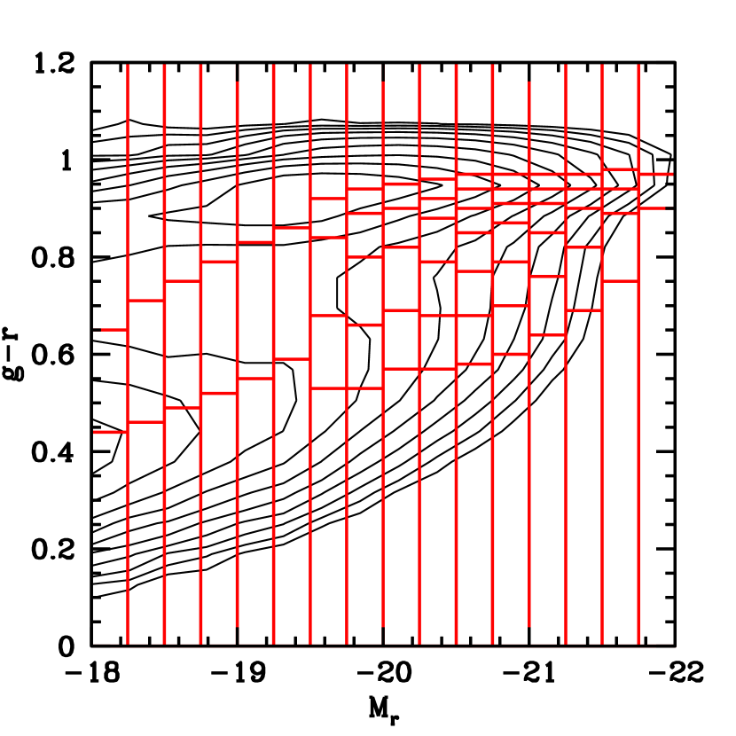
Figure 1: Construction of galaxy samples in fine bins of colour and luminosity. The contours show the number density of galaxies in the CMD, illustrating the colour-magnitude distribution of galaxies. The vertical red lines (plus the two vertical axes) represent the magnitude boundaries for volume-limited luminosity-bin samples, while the horizontal red lines (plus the two horizontal axes) mark the colour cuts within each luminosity-bin sample. In total, $79$ galaxy samples are constructed for clustering measurements and modelling. See the text (§ 2.1) for detail.

2.2 Galaxy Clustering Measurements

We measure the projected two-point correlation functions (projected 2PCFs) for the $79$ galaxy samples defined by fine bins in luminosity and colour.

We first evaluate the redshift-space 2PCFs $\xi(r_{\rm p},\pi)$ using the Landy-Szalay estimator (Landy & Szalay, 1993),

$$\xi(r_{\rm p},\pi)=\frac{{\rm DD}-2{\rm DR}+{\rm RR}}{\rm RR},$$ (1)

where $r_{\rm p}$ ($\pi$) is the galaxy pair separation perpendicular (parallel) to the line of sight, and DD, RR, and RR are the normalised numbers of data-data, data-random, and random-random galaxy pairs in the corresponding bins around $r_{p}$ and $\pi$. We adopt uniform $r_{\rm p}$ bins in logarithmic space with a bin width $\Delta\log r_{\rm p}=0.2$, with $r_{p}$ ranging from $0.13h^{-1}{\rm Mpc}$ to $20.48h^{-1}{\rm Mpc}$. The $\pi$ bins are uniform in linear space from $0$ to $40h^{-1}{\rm Mpc}$ with a bin width $\Delta\pi=2h^{-1}{\rm Mpc}$. To account for the survey geometry and angular selection function, we use the random catalogues from the NYU-VAGC. The corresponding random catalogue for each galaxy sample contains $\sim$50 times as many galaxies.

The projected 2PCF $w_{\rm p}$ is obtained by integrating the $\xi(r_{\rm p},\pi)$ along the $\pi$ direction,

$$w_{\rm p}(r_{\rm p})=2\int_{0}^{\pi_{\rm max}}d\pi\xi(r_{\rm p},\pi),$$ (2)

with $\pi_{\rm max}=40h^{-1}{\rm Mpc}$. The projected 2PCF has the redshift-space distortion effects largely removed and represents the galaxy clustering in real space. As shown later, our model accounts for any residual redshift-space distortion effects caused by a finite $\pi_{\rm max}$.

We adopt the sample mean from jackknife re-sampling method as our estimation of $w_{\rm p}$, which has no noticeable difference from that estimated with the full sample. The covariance matrix is also estimated with the jackknife method. The footprint of the galaxy sample is divided into $N=144$ spatially contiguous and equal area sub-regions. We measure $w_{\rm p}$ for $144$ times leaving out one different sub-region at each time, and the covariance is calculated as $143$ times the variance of the $144$ measurements (e.g. Zehavi et al., 2005b, 2011; Guo et al., 2015; Xu et al., 2016; Zu & Mandelbaum, 2016; Guo et al., 2017).

At a fixed magnitude bin, different colour sub-samples share the same survey volume (section 2.1), and hence the measurements of their projected 2PCFs are strongly correlated. In this work, we take into account the covariance of the $w_{\rm p}$ measurements among all the colour sub-samples at a fixed magnitude bin. In practice, galaxy samples in the adjacent magnitude bins partially overlap in volume so that their $w_{\rm p}$ measurements should also be correlated. Ideally, one would like to have a big covariance matrix to account for the correlations among $w_{\rm p}$ measurements from all galaxy samples, which would have $948\times 948$ elements (12 data points per sample times 79 galaxy samples). However, to have a precise estimation of such a covariance matrix is not practical, especially with only $144$ jackknife sub-samples. We therefore neglect the covariance for $w_{\rm p}$ measurements of samples across different magnitude bins.

In this paper, as the first step of CCMD modelling, we limit ourselves to constrain the model with auto-correlation functions. The constraints can be tested and further tightened with other clustering statistics, such as cross-correlation functions and galaxy lensing measurements. See § 5 for more discussion.

3 Conditional Colour-Magnitude Distribution (CCMD) Parametrization & Global Modelling of Colour-Luminosity Dependent Galaxy Clustering

Within the HOD/CLF framework, modelling the luminosity-dependent galaxy clustering has become a routine procedure. The halo occupation function for a luminosity-bin or luminosity-threshold galaxy sample can be obtained through an integral over the CLF (e.g. Yang et al., 2003). With the HOD approach, the halo occupation function for a luminosity-threshold sample is well parametrized (e.g. Kravtsov et al., 2004; Zheng et al., 2005, 2007), and that for a luminosity-bin sample can be obtained by differencing those of two threshold samples (e.g. Zehavi et al., 2005a, 2011). For modelling the colour-dependent galaxy clustering, most previous work adopts simple parametrizations on the red/blue fraction (e.g. Zehavi et al., 2005a), on relating colours to satellite fraction (e.g. Zehavi et al., 2011), or on colour distribution (e.g. Skibba & Sheth, 2009).

To model the luminosity-colour dependent clustering of galaxies in fine bins of luminosity and colour over the whole galaxy CMD, parametrizing the HOD of each individual sample of galaxies would be ineffective. First, the total number of parameters in the model would be large. For example, even if we apply 5 parameters for each sample, we would end up with a total of nearly 400 parameters for the $\sim 79$ samples. Second, it is difficult to make the parametrizations and the modelling results of individual samples fully compatible with each other. For example, at a fixed halo mass, over a sufficiently large luminosity range, the mean occupation numbers of central galaxies from different samples should have the constraint of adding up to unity, which may not be the case if samples are modelled individually.

A better strategy to model the luminosity-colour dependent clustering is to develop a global parametrization of the galaxy-halo relation. Here ‘global’ means that we describe the overall galaxy distribution as a function of galaxy luminosity/colour and halo mass, not those of individual samples. Then the halo occupation for each individual sample can be derived based on the luminosity and colour cuts of the sample. The global paramerization can avoid the two above problems (see more details in the following subsections). For such a purpose, we introduce the formalism of the conditional colour-magnitude distribution (CCMD), which parametrizes the colour and luminosity distribution of galaxies as a function of halo mass. It can be regarded as a substantial extension to the CLF formalism, which parameterizes the galaxy luminosity distribution as a function of halo mass. The CCMD adds the dimension of galaxy colour and describes its distribution. As with previous work (e.g. Kravtsov et al., 2004; Zheng et al., 2005) the CCMD separates contributions from central and satellite galaxies. Motivated by the bimodal colour distribution of galaxies, the CCMD also divides galaxies into red-like and blue-like populations (dubbed as pseudo-red and pseudo-blue, respectively; see below). We describe the CCMD parameterization of the four populations, pseudo-red and pseudo-blue central galaxies (§ 3.1) and pseudo-red and pseudo-blue satellite galaxies (§ 3.2).

With the CCMD parameterization, the halo occupation function can be obtained by integration for any galaxy sample given its colour and luminosity cuts. We then employ an accurate and fast method based on a $N$-body simulation to compute the model 2PCFs (§ 3.3) and use the Markov Chain Monte Carlo (MCMC) to explore the CCMD parameter space from jointly modelling the clustering measurements of the 79 SDSS galaxy samples.

3.1 CCMD of Central Galaxies

In general, the CCMD of galaxies is made of two parts, the description of colour and magnitude distribution of galaxies at a fixed halo mass and then the parameterization of the key features of that distribution as a function of halo mass.

For central galaxies, at fixed halo mass, the CLF is usually modelled as a log-normal function in luminosity or a Gaussian function in magnitude (e.g. Yang et al., 2003), which is supported by the results from the SDSS group catalogue (Yang et al., 2008). At fixed luminosity, the bimodal colour distribution of galaxies can be well described by a superposition of two Gaussian components (e.g. Baldry et al., 2004). The two components can be broadly referred to as ‘red’ and ‘blue’ galaxies. However, the two components can substantially overlap with each other. To avoid any possible confusion, hereafter we will call them pseudo-red and pseudo-blue components, and the usual red and blue samples can be defined by choosing a cut in colour.

The above descriptions of luminosity and colour distribution motivate us to model the colour-magnitude distribution of central galaxies of each pseudo-colour component at a fixed halo mass as a 2D Gaussian distribution. We need 5 numbers to describe a two-dimensional (2D) normalised Gaussian function: the centre (2 numbers), the width (2 numbers, each for one direction), and the correlation (i.e. to describe the orientation of the contours corresponding to the 2D Gaussian distribution). There are then 10 numbers from the two 2D Gaussian functions for the pseudo-red and pseudo-blue central galaxies. As we require the sum of the number of central galaxies to be unity at fixed halo mass, we also need a number to describe the the relative fraction of pseudo-red and pseudo-blue central galaxies. We parameterize it as the fraction $f_{\rm p-red}$ of pseudo-red central galaxies, and the fraction of pseudo-blue central galaxies is simply $f_{\rm p-blue}=1-f_{\rm p-red}$. In total, we have 11 numbers to describe the colour-magnitude distribution of central galaxies at a fixed halo mass.

For the convenience of presentation, we refer to the magnitude direction as the $x$ direction and the colour direction as the $y$ direction. The differential colour-magnitude distribution of each pseudo-colour central galaxy component can be written as

$$\frac{{\rm d}^{2}\langle N_{\textrm{cen, comp}}\rangle}{\rm dx\,dy}=f_{\rm comp}\frac{1}{2\pi\sigma_{\rm x}\sigma_{\rm y}\sqrt{1-\rho^{2}}}\exp\left[-\frac{Z^{2}}{2(1-\rho^{2})}\right],$$ (3)

with

$$Z^{2}=\frac{(x-\mu_{\rm x})^{2}}{\sigma^{2}_{\rm x}}+\frac{(y-\mu_{\rm y})^{2}}{\sigma^{2}_{\rm y}}-\frac{2\rho(x-\mu_{\rm x})(y-\mu_{\rm y})}{\sigma_{\rm x}\sigma_{\rm y}}$$ (4)

and

$$\rho=\frac{Cov(x,y)}{\sigma_{\rm x}\sigma_{\rm y}}.$$ (5)

Here ‘comp’ is ‘p-red’ (‘p-blue’) for the pseudo-red (pseudo-blue) population, $\mu_{\rm x}$ is the mean magnitude, $\mu_{\rm y}$ is the mean colour, $\sigma_{\rm x}$ and $\sigma_{\rm y}$ are the standard deviations in magnitude and colour, and $\rho$ ($Cov(x,y)$) is the coefficient of the correlation (covariance) between magnitude and colour.

In the CCMD framework, the above $11$ numbers for the colour-magnitude distribution of central galaxies are all functions of halo mass. We parameterize the halo mass dependence for each of them with motivations based on previous work. For each pseudo-colour central galaxy population, we first parameterize the halo-mass dependent mean and scatter in magnitude. From modelling the luminosity-dependent galaxy clustering with SDSS DR7, Zehavi et al. (2011) obtains an empirical relation between median luminosity $L_{\textrm{cen}}$ of central galaxies and halo mass $M_{\rm h}$ (see Eq.11 in their paper):

$$L_{\textrm{cen}}=L_{\rm t}\left(\frac{M_{\rm h}}{M_{\rm t}}\right)^{\alpha_{\rm M}}\exp\left(-\frac{M_{\rm t}}{M_{\rm h}}+1\right),$$ (6)

which describes the relation as a power law with an exponential cutoff towards the low halo mass end and is characterised by the high-mass end power-law index $\alpha_{\rm M}$, the transition (cutoff) mass scale $M_{\rm t}$, and the median luminosity $L_{\rm t}$ at the cutoff mass scale. We adopt this functional form to parameterize the relation between the mean magnitude of central galaxies and halo mass for each pseudo-colour central galaxy population. Rewriting the equation in magnitude, we have for each central population

$$\mu_{\rm x}=x_{\rm t}-2.5\alpha_{\rm M}\log\left(\frac{M_{\rm h}}{M_{\rm t}}\right)-1.086\left(-\frac{M_{\rm t}}{M_{\rm h}}+1\right),$$ (7)

with $\mu_{\rm x}$ the mean absolute magnitude of the central galaxy population in haloes of mass $M_{\rm h}$ and $x_{\rm t}$ that in haloes of transition mass $M_{\rm t}$.

For the scatter in the magnitude of central galaxies of each population, we parameterize it to follow a linear relation with halo mass, motivated by Yang et al. (2008) (see their fig.4),

$$\sigma_{\rm x}=a_{\rm 0,\sigma_{x}}+a_{\rm 1,\sigma_{x}}(\log M_{\rm h}-\log M_{\rm nl}),$$ (8)

with two free parameters, $a_{\rm 0,\sigma_{x}}$ and $a_{\rm 1,\sigma_{x}}$. The quantity $M_{\rm nl}$ is the $z=0$ nonlinear mass for collapse, and for our adopted cosmology $\log[M_{\rm nl}/(h^{-1}{\rm M_{\odot}})]=12.35$. We note that the coefficient parameters use subscripts to denote the quantity to be described, and such a notation will be adopted in the following cases.

For the mean colour $\mu_{\rm y}$ and colour scatter $\sigma_{\rm y}$ of central galaxies, van den Bosch et al. (2008) show that both of them vary with galaxy magnitude monotonically. Baldry et al. (2004) introduce a hyperbolic tangent function to accurately describe the colour distribution as a function of magnitude in the galaxy CMD. We therefore parameterize both $\mu_{\rm y}$ and $\sigma_{\rm y}$ as a function of the mean magnitude $\mu_{\rm x}$, which is then linked to halo mass. With the insights from Baldry et al. (2004) and van den Bosch et al. (2008), we express each as a combination of a linear function and a hyperbolic tangent function,

$$\mu_{\rm y}=a_{\rm 0,y}+a_{\rm 1,y}(\mu_{\rm x}-\mu_{\ast})+q_{\rm 0,y}\textrm{tanh}\left(\frac{\mu_{\rm x}-q_{\rm 1,y}}{q_{\rm 2,y}}\right)$$ (9)

and

$$\sigma_{\rm y}=a_{\rm 0,\sigma_{y}}+a_{\rm 1,\sigma_{y}}(\mu_{\rm x}-\mu_{\ast})+q_{\rm 0,\sigma_{y}}\rm{tanh}\left(\frac{\mu_{x}-q_{\rm 1,\sigma_{y}}}{q_{\rm 2,\sigma_{y}}}\right),$$ (10)

where $a$’s and $q$’s are free parameters and $\mu_{*}=-20.44$ corresponds to the $r$-band characteristic luminosity in the local galaxy LF (Blanton et al., 2003a).

The correlation $\rho$ between central galaxy luminosity and colour at fixed halo mass is not well constrained in the literature. We propose a linear relation to describe its halo mass dependence,

$$\rho=a_{\textrm{0,$\rho$}}+a_{\textrm{1,$\rho$}}(\log M_{h}-\log M_{\rm nl}),$$ (11)

with $a_{\textrm{1,$\rho$}}$ and $a_{\textrm{0,$\rho$}}$ as the two free parameters.

For the fraction of pseudo-red central galaxies, the galaxy CMD suggests that it increases with increasing galaxy luminosity and hence halo mass. We parameterize it with a ramp-like function,

$$f_{\textrm{p-red}}=\frac{1}{2}a_{\textrm{0,f}}\left[1+\textrm{erf}\left(\frac{\log M_{h}-a_{\textrm{2,f}}}{a_{\textrm{1,f}}}\right)\right],$$ (12)

where ${\rm erf}$ is the error function.

In summary, the colour-magnitude distribution of central galaxies is described as a combination of contributions from two galaxy populations, the pseudo-red and pseudo-blue central galaxies. At fixed halo mass, the distribution of each population is modelled as a 2D Gaussian. The halo-mass dependences of the quantities in each 2D Gaussian function are described with 17 parameters: 3 for the mean magnitude ($x_{\rm t}$, $M_{\rm t}$, and $\alpha_{\rm M}$; Eq. 7), 2 for the scatter in magnitude ($a_{0,\sigma_{\rm x}}$ and $a_{1,\sigma_{\rm x}}$; Eq. 8), 5 for the mean colour ($a_{\rm 0,y}$, $a_{\rm 1,y}$, $q_{\rm 0,y}$, $q_{\rm 1,y}$, and $q_{\rm 2,y}$; Eq. 9), 5 for the scatter in colour ($a_{\rm 0,\sigma_{y}}$, $a_{\rm 1,\sigma_{y}}$, $q_{\rm 0,\sigma_{y}}$, $q_{\rm 1,\sigma_{y}}$, and $q_{\rm 2,\sigma_{y}}$; Eq. 10), and 2 for the colour-magnitude correlation ($a_{0,\rho}$ and $a_{1,\rho}$; Eq. 11). Therefore, the two 2D Gaussian functions for the two central galaxy populations have 34 parameters. There are also 3 parameters ($a_{\rm 0,f}$, $a_{\rm 1,f}$, and $a_{\rm 2,f}$; Eq. 12) in the fraction of the pseudo-red central galaxies, which specifies the relative normalisation of the two Gaussian functions. In total, we use 37 parameters to describe the CCMD of central galaxies. The halo-mass dependences of the parameters describing central galaxies in the best-fit model are illustrated in Fig. 12.

3.2 CCMD of Satellite Galaxies

For satellite galaxies, we also divide their CCMD into contributions from two populations, namely the pseudo-blue and pseudo-red satellite galaxies.

Using a group catalogue, Yang et al. (2008) study the CLFs of blue and red satellite galaxies and find that each can be well described by a modified Schechter function

$$\frac{d\langle N_{\textrm{sat}}\rangle}{d\log L}=\phi_{\rm s}\left(\frac{L}{L_{\rm s}^{\ast}}\right)^{\alpha_{\rm s}+1}\exp\left[-\left(\frac{L}{L_{\rm s}^{\ast}}\right)^{2}\right],$$ (13)

where $\phi_{\rm s}$ is the normalisation, $\alpha_{\rm s}$ is the faint-end slope, and $L_{\rm s}^{\ast}$ is the characteristic luminosity where the CLF transits from a power-law form to an exponential form.

We adopt the above CLF form and add the colour dimension to construct the luminosity and colour distribution of satellite galaxies for each pseudo-colour population. Motivated by the double-Gaussian fit to the galaxy colour distribution at fixed luminosity, we assume that for each population satellite colour follows a Gaussian distribution at fixed luminosity. In terms of absolute magnitude and colour, the satellite CCMD at fixed halo mass for a pseudo-colour population reads

$$\frac{{\rm d}^{2}\langle N_{\textrm{sat,comp}}\rangle}{\rm dx\,dy}=\frac{1}{\sqrt{2\pi}\sigma_{\textrm{y,sat}}}\exp\left[-\frac{(y-\mu_{\textrm{y,sat}})^{2}}{2\sigma^{2}_{\textrm{y,sat}}}\right]\\ \times 0.4\phi_{\rm s}10^{-0.4(\alpha_{\rm s}+1)(x-x_{\rm s}^{\ast})}\exp\left[-10^{-0.8(x-x_{\rm s}^{\ast})}\right],$$ (14)

where $x_{\rm s}$ is the absolute magnitude corresponding to $L_{\rm s}^{\ast}$, the Gaussian function represents the colour distribution (see below), and similar to the case with central galaxies ‘comp’ here can be either ‘p-blue’ or ‘p-red’.

Each quantity on the right-hand side of the above equation varies with halo mass, which needs to be parameterized. As suggested in Yang et al. (2008) and van den Bosch et al. (2013), a quadratic function of halo mass is a good description for the halo-mass dependence of either the normalisation $\phi_{\rm s}$ and the faint-end slope $\alpha_{\rm s}$. Therefore we adopt the following parameterizations,

$$\log\phi_{\rm s}=a_{\textrm{0,$\phi$}}+a_{\textrm{1,$\phi$}}(\log M_{\rm h}-\log M_{\rm nl})\\ +a_{\textrm{2,$\phi$}}(\log M_{\rm h}-\log M_{\rm nl})^{2}$$ (15)

and

$$\alpha_{\rm s}=a_{\textrm{0,$\alpha$}}+a_{\textrm{1,$\alpha$}}(\log M_{\rm h}-\log M_{\rm nl})\\ +a_{\textrm{2,$\alpha$}}(\log M_{\rm h}-\log M_{\rm nl})^{2},$$ (16)

where the $a$’s are free parameters.

Yang et al. (2008) suggest that there is a luminosity gap between the median luminosity of central galaxy $L_{\textrm{cen}}$ and the characteristic luminosity $L_{\rm s}^{\ast}$ of satellite galaxies independent of halo mass. In terms of absolute magnitude, we have

$$x_{\rm s}^{\ast}=\mu_{x}+\Delta_{\rm sc},$$ (17)

where $\Delta_{\rm sc}$ (independent of halo mass) is the luminosity gap in absolute magnitude. This $\Delta_{\rm sc}$ parameter and the halo-mass dependent $\mu_{\rm x}$ (Eq. 7) give our parameterization of the dependence of $x_{\rm s}^{\ast}$ on halo mass.

The mean and standard deviation of the colour of satellite galaxies is found to follow a linear relation with stellar mass (van den Bosch et al., 2008). Motivated by this result, we parameterize the mean and standard deviation of the satellite colour through luminosity,

$$\mu_{\textrm{y,sat}}=a_{\textrm{0,y,sat}}+a_{\textrm{1,y,sat}}(x-\mu_{\ast})$$ (18)

and

$$\sigma_{\textrm{y,sat}}=a_{\textrm{0, $\sigma_{\textrm{y,sat}}$}}+a_{\textrm{1, $\sigma_{\textrm{y,sat}}$}}(x-\mu_{\ast}),$$ (19)

where the $a$’s are parameters to link the satellite colour distribution with the magnitude and $\mu_{\ast}=-20.44$ corresponds to the characteristic luminosity in the $r$-band LF of local galaxies (Blanton et al., 2003a).

In summary, in the parameterization of the satellite CCMD, we introduce parameters related to the CLF and satellite colour distribution. For each pseudo-colour satellite population, there are 7 parameters to describe the CLF as a function of halo mass: 3 for $\phi_{\rm s}$ ($a_{0,\phi}$, $a_{1,\phi}$, and $a_{2,\phi}$; Eq. 15), 3 for $\alpha_{\rm s}$ ($a_{0,\alpha}$, $a_{1,\alpha}$, and $a_{2,\alpha}$; Eq. 16, and 1 for $x_{\rm s}$ ($\Delta_{\rm sc}$; Eq. 17). There are 4 parameters to characterise the satellite colour distribution: 2 for the mean $\mu_{\rm y,sat}$ ($a_{\rm 0,y,sat}$ and $a_{\rm 1,y,sat}$; Eq. 18) and 2 for the scatter $\sigma_{\rm y,sat}$ ($a_{\rm 0,\sigma_{y,sat}}$ and $a_{\rm 1,\sigma_{y,sat}}$; Eq. 19). Overall, we end up with 22 free parameters to describe the CCMD of the satellite population (pseudo-blue plus pseudo-red). The halo-mass dependences of the parameters describing satellite galaxies in the best-fit model are illustrated in Fig. 13.

Together with the 37 parameters introduced in the CCMD of central galaxies, we have a total of 59 parameters to fully connect the colour-magnitude distribution of galaxies with halo mass. At first glimpse, the total number of parameters is large. However, we note that the parameterization is intended to cover the whole range of the galaxy CMD in Fig. 1, not for a single galaxy sample. With this global parameterization, the halo occupation function for each of the 79 galaxy samples we construct can be obtained by integrating the CCMD over the range of the colour and magnitude cuts of the sample. Instead of the global parameterization, if the model were built by parameterizing each individual sample with, say, 5 parameters, we would end up with $\sim 400$ parameters in total. Therefore the number of parameters in our global parameterization in fact is small, about 59/79$\sim$0.7 parameter per sample. Furthermore, with the global parameterization, no inconsistency would arise among the halo occupations of different samples, which avoids a problem seen in the results from individual parameterizations of different samples (e.g. Zheng et al., 2007). We will use a total of 948 data points to constrain these 59 parameters.

3.3 Calculation of Projected 2PCFs and CCMD Modelling of Galaxy Clustering

With the global parameterization of the CCMD of galaxies, for a given galaxy sample, the mean occupation function (separated into central and satellite contributions) can be obtained by integrating the CCMD within the boundary set by the sample’s colour and magnitude cuts. We then adopt the accurate and efficient method laid out in Zheng & Guo (2016) to compute the projected 2PCF for each sample.

The basic idea of the method is to tabulate all the necessary information for computing the various 2PCF components, using dark matter haloes identified in an $N$-body simulation and within fine bins of halo mass. The galaxy 2PCF is then obtained by a simple summation over halo mass bins with the halo occupation of galaxies properly accounted for. The method is equivalent to populating galaxies into haloes to form a mock galaxy catalogue and using the 2PCF measurements from the mock as the model predictions, which ensures the accuracy of the calculation. The calculation is also fast, enabling an efficient exploration of the HOD or CCMD parameter space.

In detail, we use haloes identified in the MultiDark simulation with Planck cosmology. We assume that central galaxies reside at the potential minimum of haloes and satellite galaxies follow the spatial distribution of dark matter particles inside haloes. Rather than determining the positions of satellites in a halo based on a radial profile of analytic form, we assign the positions of randomly chosen dark matter particles to satellites. Then with the simulation, the following quantities are measured in fine bins of halo mass: $\bar{n}_{i}$, the number density of haloes in the $i$-th mass bin (mass $M_{i}$); $f_{\rm cs}(\boldsymbol{r};M_{i})$, the normalised central-satellite pair distribution profile in haloes of mass $M_{i}$, calculated using the positions of the potential minimum (position to put the central galaxy) and dark matter particles (positions for satellite galaxies) in each halo; $f_{\rm ss}(\boldsymbol{r};M_{i})$, the normalised satellite-satellite pair distribution profile in haloes of mass $M_{i}$, calculated using the positions of dark matter particles in each halo; $\xi_{\rm hh,cc}(\boldsymbol{r};M_{i},M_{j})$, the two-point cross-correlation function between haloes of masses $M_{i}$ and $M_{j}$, where halo positions come from the potential minimum (positions to put central galaxies); $\xi_{\rm hh,cs}(\boldsymbol{r};M_{i},M_{j})$, the two-point cross-correlation function between haloes of masses $M_{i}$ and $M_{j}$, where for each halo pair the position of the potential minimum (position to put a central galaxy) of one halo and the position of a random dark matter particle (position to put a satellite galaxy) in the other halo are used; $\xi_{\rm hh,ss}(\boldsymbol{r};M_{i},M_{j})$, the two-point cross-correlation function between haloes of masses $M_{i}$ and $M_{j}$, where the positions of dark matter particles (positions to put satellite galaxies) are used.

The above quantities are all calculated in redshift space (i.e. with $\boldsymbol{r}$ the redshift-space pair separation vector) with the same binning scheme as used in our measurements of the SDSS galaxy clustering. Then we integrate each component along the line of sight to obtain the projected counterpart for the projected 2PCF. That is,

$$w_{\rm f,cs}(r_{\rm p};M_{i})=2\int_{0}^{\pi_{\rm max}}{\rm d}\pi\,f_{\rm cs}(r_{\rm p},\pi;M_{i}),$$ (20)

$$w_{\rm f,ss}(r_{\rm p};M_{i})=2\int_{0}^{\pi_{\rm max}}{\rm d}\pi\,f_{\rm ss}(r_{\rm p},\pi;M_{i}),$$ (21)

$$w_{\rm hh,cc}(r_{\rm p};M_{i},M_{j})=2\int_{0}^{\pi_{\rm max}}{\rm d}\pi\,\xi_{\rm hh,cc}(r_{\rm p},\pi;M_{i},M_{j}),$$ (22)

and similarly for $w_{\rm hh,cs}(r_{\rm p};M_{i},M_{j})$ and $w_{\rm hh,ss}(r_{\rm p};M_{i},M_{j})$. Those $w$’s and $\bar{n}_{i}$ are tabulated. The projected 2PCF $w_{\rm p}(r_{\rm p})$ for a given galaxy sample is the sum of the one-halo and two-halo terms (contributed by intra-halo and inter-halo galaxy pairs, respectively), $w_{\rm p}(r_{\rm p})=w_{\rm p}^{\rm 1h}(r_{\rm p})+w_{\rm p}^{\rm 2h}(r_{\rm p})$. The two terms are calculated as (Zheng & Guo, 2016)

$$w_{\rm p}^{\rm 1h}(r_{\rm p})=\sum_{i}2\frac{\bar{n}_{i}}{\bar{n}_{\rm g}^{2}}\langle N_{\rm cen}(M_{i})N_{\rm sat}(M_{i})\rangle w_{\rm f,cs}(r_{\rm p};M_{i})\\ +\sum_{i}\frac{\bar{n}_{i}}{\bar{n}_{\rm g}^{2}}\langle N_{\rm sat}(M_{i})[N_{\rm sat}(M_{i})-1]\rangle w_{\rm f,ss}(r_{\rm p};M_{i})$$ (23)

and

$$w_{\rm p}^{\rm 2h}(r_{\rm p})=\sum_{i,j}\frac{\bar{n}_{i}\bar{n}_{j}}{\bar{n}_{\rm g}^{2}}\langle N_{\rm cen}(M_{i})\rangle\langle N_{\rm cen}(M_{j})\rangle w_{\rm hh,cc}(r_{\rm p};M_{i},M_{j})\\ +\sum_{i,j}2\frac{\bar{n}_{i}\bar{n}_{j}}{\bar{n}_{\rm g}^{2}}\langle N_{\rm cen}(M_{i})\rangle\langle N_{\rm sat}(M_{j})\rangle w_{\rm hh,cs}(r_{\rm p};M_{i},M_{j})\\ +\sum_{i,j}\frac{\bar{n}_{i}\bar{n}_{j}}{\bar{n}_{\rm g}^{2}}\langle N_{\rm sat}(M_{i})\rangle\langle N_{\rm sat}(M_{j})\rangle w_{\rm hh,ss}(r_{\rm p};M_{i},M_{j}),$$ (24)

where $\bar{n}_{\rm g}=\sum_{i}\bar{n}_{i}[\langle N_{\rm cen}(M_{i})\rangle+\langle N_{\rm sat}(M_{i})\rangle]$ is the number density of the galaxy sample. The mean occupation functions of central and satellite galaxies, $\langle N_{\rm cen}(M)\rangle$ and $\langle N_{\rm sat}(M)\rangle$, are computed through integrating the CCMD with the integral limits set by the colour and magnitude cuts of the given sample. For the mean number of one-halo central-satellite pairs in haloes of mass $M_{i}$ (Eq. 23), we assume that there is no correlation between central and satellite galaxies, which leads to $\langle N_{\rm cen}(M_{i})N_{\rm sat}(M_{i})\rangle=\langle N_{\rm cen}(M_{i})\rangle\langle N_{\rm sat}(M_{i})\rangle$. For the mean number of one-halo satellite-satellite pairs (Eq. 23), we assume that the number of satellites follows a Poisson distribution, meaning that $\langle N_{\rm sat}(M_{i})[N_{\rm sat}(M_{i})-1]\rangle=\langle N_{\rm sat}(M_{i})\rangle^{2}$.

As the model follows the same binning and integration procedure as in the observation, it is immune to any effect caused by binning and any residual redshift-space distortion is automatically accounted for. That is, the computed projected 2PCF for a given galaxy sample is equivalent to that measured in a mock galaxy catalogue from populating haloes with the corresponding HOD (Zheng & Guo, 2016).

The tables are computed with Rockstar haloes (Behroozi et al., 2013) from the MultiDark MDPL2 simulation. The MDPL2 simulation (Klypin et al., 2016) assumes a spatially flat cosmology consistent with the constraints from Planck (Planck Collaboration et al., 2014, 2016), with $\Omega_{\rm m}=0.307$, $\Omega_{\rm b}=0.048$, $h=0.678$, $n_{\rm s}=0.96$, and $\sigma_{8}=0.823$. The simulation has a box size of $1h^{-1}{\rm Gpc}$ (comoving) on a side with $3840^{3}$ particles. With the corresponding mass resolution of $1.51\times 10^{9}h^{-1}{\rm M_{\odot}}$, there are about 100 particles per halo at the low mass end relevant for our modelling and the simulation is well suited for modelling the clustering measurements of the galaxy samples we construct. We note that the halo mass we adopt in this work is the virial mass $M_{\rm vir}$. There is a small offset between $M_{\rm vir}$ and $M_{\rm 200b}$, where $M_{\rm 200b}$ is the halo mass with haloes defined as having mean density of 200 times that of the background universe. Based on the MDPL2 halo catalogue, we find that the mean offset can be well described as $\log M_{\rm 200b}-\log M_{\rm vir}=0.0052(\log M_{\rm vir}-13.5)+0.0498$, where halo mass is in units of $h^{-1}M_{\odot}$. This offset will be applied when we make comparisons with some results in previous work.

To constrain the CCMD, we model the clustering measurements and number densities of the 79 galaxy samples in fine bins of colour and magnitude. The $\chi^{2}$ is constructed as

$$\chi^{2}=(\boldsymbol{w_{\rm p}}-\boldsymbol{w^{\ast}_{\rm p}})^{\rm T}\boldsymbol{\sf{C^{-1}_{w_{\rm p}}}}(\boldsymbol{w_{\rm p}}-\boldsymbol{w^{\ast}_{\rm p}})\\ +(\boldsymbol{n_{\rm g}}-\boldsymbol{n^{\ast}_{\rm g}})^{\rm T}\boldsymbol{\sf{C^{-1}_{n_{\rm g}}}}(\boldsymbol{n_{\rm g}}-\boldsymbol{n^{\ast}_{\rm g}}),$$ (25)

where $\boldsymbol{w_{\rm p}}$ ($\boldsymbol{w^{\ast}_{\rm p}}$) and $\boldsymbol{n_{\rm g}}$ ($\boldsymbol{n^{\ast}_{\rm g}}$) are the 2PCF and number density model (data) vectors from all the samples, and $\boldsymbol{\sf{C_{w_{\rm p}}}}$ and $\boldsymbol{\sf{C_{n_{\rm g}}}}$ are the corresponding covariance matrices. The covariances among samples within the same magnitude bin (hence the same survey volume) have been accounted for (see § 2.2).

There is noise in the covariance matrix for galaxy samples in each luminosity bin as it is estimated with a limited number of jackknife sub-samples. To reduce the effect of noise, we apply the singular-value decomposition (SVD) technique to the normalised covariance matrix and remove eigenvalues smaller than $\sqrt{2/N}$ (e.g. Gaztañaga & Scoccimarro, 2005; Sinha et al., 2018), where $N=144$ is the number of jackknife sub-samples. This SVD procedure effectively reduces the data points, and we end up with 897 effective data points (818 $w_{\rm p}$ and 79 $n_{\rm g}$ points). To account for the mean bias in inverting the matrix, we also scale the inverse matrix by $(N-N_{\rm dom}-2)/(N-1)$, a correction proposed by Hartlap et al. (2007), where $N_{\rm dom}$ is the number of effective data points.

With the likelihood of the model given the data, which is proportional to $\exp(-\chi^{2}/2)$, we employ the MCMC method to explore the CCMD parameter space. Flat priors in linear space are adopted for all the parameters. Given the large dimension of the parameter space (59 parameters; see § 3), we typically require the length of the chain to be about $10^{8}$ and the convergence is tested by comparing the results from different realisations of chains. We present additional tests of the results in Appendix B.

4 CCMD Modelling Results

With the CCMD parameterization, we simultaneously model the clustering measurements and number densities of the 79 samples of galaxies in fine bins of colour and magnitude. The minimum $\chi^{2}$ from the MCMC chain is found to be $952$. Given the number of the degrees of freedom $n_{\rm d.o.f.}=818+79-59=838$ (818 effective $w_{\rm p}$ points plus 79 $n_{\rm g}$ points and 59 CCMD parameters), the expected 1$\sigma$ range of the $\chi^{2}$ distribution is $838\pm 41$. The minimum $\chi^{2}$ we find is within the 2.8$\sigma$ range. See Appendix B for more tests with parameter constraints.

In this section, we present the modelling results. We start with an assessment on how well the model works by comparing the observables inferred from the model and those from the observational data. We then focus on the constraints on the CCMD parameters and inferred quantities and relations. Finally we compare different aspects of the galaxy-halo connection inferred from our model with previous work.

We note that by design the CCMD model implements no galaxy assembly bias effect, as the distribution of galaxy luminosity and colour is assumed to only depend on halo mass, not other halo properties that are related to halo environment and assembly history. Therefore the modelling results and the subsequent galaxy-halo connection presented in this paper are valid under such an assumption. For future work, we can extend the framework to parameterize the galaxy-halo relation to depend on an environment or assembly sensitive halo property, which would incorporate a certain form of assembly bias. As we discuss in section 5, our modelling results here, in combination with observational data, can help reveal and constrain galaxy assembly bias.

4.1 Observation versus Model

Figure 2: Comparison of galaxy abundances in the CMD between observation and best-fitting model prediction. The left panel shows the measured galaxy number density distribution calculated in fine bins of galaxy colour and magnitude, for bins with $p_{\rm g}\geq 10^{-3.0}h^{3}{\rm Mpc}^{-3}/{\rm mag}^{2}$, where $p_{\rm g}\equiv{\rm d}^{2}n_{g}/{\rm dM_{r}/d(g-r)}$ is the number density of galaxies per magnitude per colour. The middle panel shows the corresponding distribution from the best-fitting CCMD model. In the right panel, the colour scale shows the fractional difference in galaxy number density distribution between model and observation, $(p_{\textrm{g,model}}-p_{\textrm{g,data}})/p_{\textrm{g,data}}$, while the magenta and black contours are the observed and model distribution of galaxy abundance.

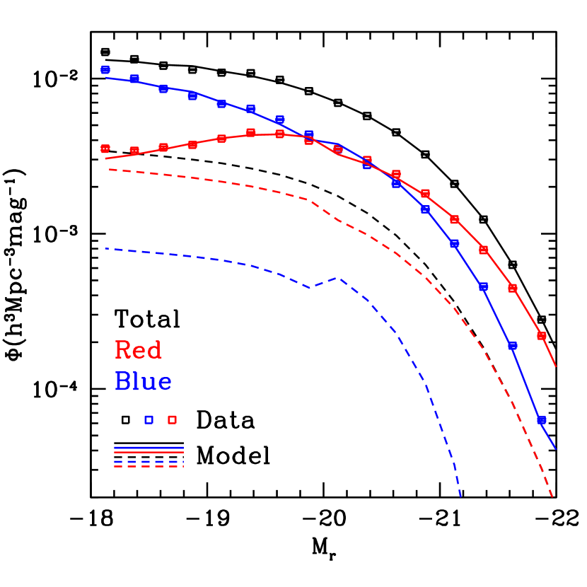
Figure 3: Comparison of observed and model galaxy LFs. The black data points show the observed LFs of all the galaxies, which is further separated into that of blue galaxies (blue) and that of red galaxies (red). The solid curves are the corresponding LFs from the best-fitting CCMD model, and the dashed curves are the predicted contributions from satellites. A luminosity-dependent colour cut is adopted to divide galaxies into blue and red populations (Zehavi et al. 2011; see text § 4.1 for detail).

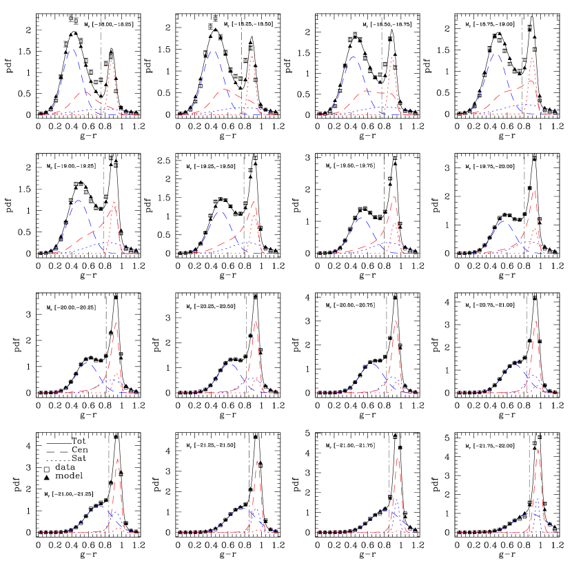
Figure 4: Comparison of luminosity-dependent galaxy colour distribution from observation and model. In each panel, the squares are the observed probability distribution function (PDF) of galaxy colour for a given luminosity bin (indicated inside each panel). The solid curve is the PDF from the best-fitting model, while the triangles are the model PDF integrated over the same colour bins as used in the observation. The blue/red dashed and dotted curves are the contributions from central and satellite galaxies of the pseudo-blue/pseudo-red populations in the model (see text for detail). In each panel, the vertical line indicates the luminosity-dependent colour cut (Zehavi et al., 2011) to divide galaxies into blue and red populations in observation.

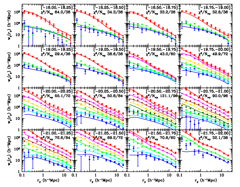
Figure 5: Comparison of the projected 2PCFs between observation and model. Each panel shows the colour-dependent projected 2PCFs for a given luminosity bin (marked in the top-right corner). The filled circles represent the measurements from the observational data and the solid curves stand for those from the best-fitting CCMD model. For clarity, offsets are added to both the data and model to separate galaxy sub-samples of different colours and error bars are only plotted for the bluest and reddest samples. The value of $\chi^{2}$ computed using the $w_{\rm p}$ data in the panel is labelled, together with the number of $w_{\rm p}$ data points, which is meant to aid the comparison between data and model (see text § 4.1 for detail).

As the model is based on fitting the number densities and 2PCFs of the 79 galaxy samples in fine bins of colour and magnitude across the galaxy CMD, we expect that the bimodal distribution in the CMD is well captured by the model. In Fig. 2, we compare the galaxy CMD from observation and that from the best-fitting model. To resolve the key features in the CMD, we use much finer colour bins (0.06 mag) than the ones adopted in the modelling, which put the model under a more stringent test. The model passes such a check and reasonably reproduces the overall CMD. The right panel shows the fractional differences between the model and data. The model works well for luminous galaxies, especially those more luminous than $L^{\ast}$. These galaxy samples have large survey volumes and thus small fractional uncertainties in their 2PCF measurements. Also for these samples, we are able to construct sub-samples with finer colour bins. Both factors contribute to the tight constraints on the CCMD model in the corresponding regions of the parameter space. For faint galaxies, especially those fainter than $M_{\rm r}\sim-19$, the difference between model and data increases. Besides the small survey volume and relatively large uncertainties in the 2PCF and number density measurements, the coarse colour bins (e.g. 3 colour subsamples at fixed magnitude) also contribute to the increased difference. Fitting the number densities of the coarse-colour sub-samples well does not guarantee that the model can do well in predicting those for the finer-colour-bin sub-subsamples. In our case, the worst match is in the green valley region of the faint samples, with the difference increasing to about 30 per cent.

The model reproduces the CMD reasonably well, implying that the colour-dependent galaxy LF inferred from the the model should agree with the data. Fig. 3 shows such a comparison between the model and observed galaxy LF, which is further decomposed into those from blue and red galaxies, respectively. A luminosity-dependent colour cut as in Zehavi et al. (2011) is adopted for the division between red and blue galaxies. As expected, the CCMD modelling results nicely follow the data. Only at the very faint end ($M_{\rm r}\sim-18$) and the very luminous end ($M_{\rm r}\lesssim-22$; not shown), the agreement degrades. The former reflects the loose constraints in the corresponding regions of the CCMD parameter space caused by the small survey volumes and coarse colour bins used for the modelling. The latter corresponds to samples outside of the luminosity range of modelled ones such that the model curves there are actually from extrapolation. It is encouraging that the extrapolated results are still close to the observation.

The black dashed curve in Fig. 3 shows the satellite contribution to the LF predicted by the best-fitting CCMD, which is decomposed into those from red and blue galaxies (red and blue dashed curves, respectively) with the luminosity-dependent colour cut of Zehavi et al. (2011). The satellite LF is dominated by the red galaxies over the whole luminosity range, with the fraction of red satellites increasing from $\sim$80 per cent at $M_{\rm r}\sim-18$ to 100 per cent at $M_{\rm r}\sim-22$. For red galaxies, the majority of faint ones ($\sim$90 per cent) are satellites and the fraction of satellites decreases with increasing luminosity. For blue galaxies, they are dominated by central galaxies over the whole luminosity range.

Figure 6: Similar to Fig. 5, but on the comparison of the average projected 2PCFs between observation and model. Each panel shows the average projected 2PCFs as a function of median colour of the galaxy sub-samples for a given luminosity bin (marked in the top-left corner). The filled and open circles represent the average values of the observed $w_{\rm p}(r_{\rm p})$ over the $r_{\rm p}$ ranges of 0.1–1$h^{-1}{\rm Mpc}$ (one-halo regime) and 2.51–10$h^{-1}{\rm Mpc}$ (two-halo regime), respectively. The solid and dotted curves correspond to those from the best-fitting CCMD model.

Figure 7: Similar to Fig. 6, but on the comparison of the average projected 2PCFs between observation and model for luminosity-bin samples. The filled and open circles represent the average values of the observed $w_{\rm p}(r_{\rm p})$ over the $r_{\rm p}$ ranges of 0.1–1$h^{-1}{\rm Mpc}$ (one-halo regime) and 2.51–10$h^{-1}{\rm Mpc}$ (two-halo regime), respectively. The solid and dotted curves correspond to those from the best-fitting CCMD model. See the text for the explanation of the apparent difference between the data and the model below $L^{\ast}$.

We can also take a close look at the luminosity-dependent colour distribution of galaxies, which is shown in Fig. 4. The solid curve in each panel (representing a fixed magnitude bin) is computed from the best-fitting model by accounting for the contributions from haloes of all masses. The model also gives the contributions from central/satellite galaxies of different pseudo-colour populations (dashed and dotted curves; which will be discussed in § 4.2). The open squares are the data points from observation, while the solid triangle points are from the model with the finite colour bin size effect taken into account. At low luminosity, the colour distribution profile appears to be double-peak, with a broad blue peak and a narrow red peak. For the two lowest luminosity bins, the model tends to underestimate the fraction of galaxies near the blue peak and overestimate that redder than the red peak. As the luminosity increases, the broad blue peak gradually merger with the red one. For luminous bins, the model reproduces the colour distribution remarkably well, including the overall shape and the tail distribution. In each panel, the vertical line marks the luminosity-dependent colour cut adopted in Zehavi et al. (2011) to divide galaxies into blue and red populations in observation.

With the colour and luminosity distributions well reproduced by the best-fitting model, we turn to galaxy clustering. In Fig. 5, the comparison is done between the observed and model projected 2PCFs at each luminosity bin as a function of galaxy colour (different points and curves in each panel). In each panel, the value of $\chi^{2}$ from comparing the model with the data for all the samples in the corresponding magnitude bin is shown, together with the number of data points (denoted as ‘${\rm N_{\rm wp}}$’). Although this does not represent the exact goodness of fit for $w_{\rm p}$ in each panel (as it neglects the number of parameters), the values can give a sense of how well the model works in each luminosity bin.

As a whole, the model fits the 2PCFs well for galaxy samples covering a range of $\sim$40 in luminosity (or 4 mag in magnitude) and across the full colour range (about 1.2 mag). Noticeably, the fit appears to be poor for samples with the lowest luminosity ($-18.25<M_{\rm r}<-18.00$; the bottom-left panel), which has $\chi^{2}=64$ for 36 data points. A close inspection reveals that for the blue sample the model predicts an amplitude too high compared to the data points on scales above $\sim$3$h^{-1}{\rm Mpc}$. The model also predicts lower $w_{\rm p}$ at small scales for faint samples with $M_{\rm r}>-19.5$ (except for the faintest sample; also see Fig. 7). We note that the samples with the lowest luminosity suffer the most from the small survey volume and thus have the largest sample variance (e.g. Zehavi et al., 2005a, 2011; Xu et al., 2016). The other trend we notice is that for the bluest galaxy samples with high luminosity (more luminous than $\sim L^{\ast}$ or -20.44 mag) the model tends to under-predict the clustering amplitude on scales smaller than $\sim$0.5$h^{-1}{\rm Mpc}$. Although given the large measurement uncertainties the trend appears to be weak, it systematically shows up in almost all the high luminosity bins. The model curve is flattened towards small scales, while the data seem to have an inflection and have a steep increase. This indicates that there may be too few one-halo galaxy pairs in the model. Further investigations are needed to study the clustering of the luminous blue galaxies to determine whether the trend is real and to discuss its implications.

Since offsets are added in the projected 2PCFs in Fig. 5, the luminosity and colour dependence in the 2PCF amplitude is not easily revealed. To show the trend, we compute projected 2PCF amplitudes averaged over $r_{\rm p}$ ranges of 0.1–1$h^{-1}{\rm Mpc}$ and 2.51–10$h^{-1}{\rm Mpc}$, respectively, and plot their dependence on luminosity and (median) colour of galaxy samples in Fig. 6. In detail, we compute the arithmetic mean of $N$ values of $w_{\rm p}$, $\langle w_{\rm p}\rangle=\sum_{i=1}^{N}w_{{\rm p},i}/N$, and derive the error bars from the variance in the mean, $\sigma^{2}=\sum_{i,j=1}^{N}C_{ij}/N^{2}$, where $C_{ij}$ is the covariance matrix of $w_{\rm p}$. The small-scale and large-scale averages represent the mean clustering amplitudes in the one-halo and two-halo regime.

At fixed colour, the points across different panels show the luminosity dependence, while in each panel the colour dependence at fixed luminosity is shown. We see that the clustering amplitude at both small and large scales has a stronger dependence on colour than luminosity. At fixed luminosity, the small-scale clustering amplitude shows a stronger dependence on colour than the large-scale one, indicating the strong dependence of satellite fraction on galaxy colour (see § 4.3 for more discussions). Overall, the CCMD reproduces the luminosity and colour dependent clustering amplitude (note that the data points in each panel are correlated). As with Fig. 5, the relatively large deviations between data and model are seen in the one-halo amplitude for the luminous blue galaxies (above $L^{\ast}$) and the two-halo amplitude for the faint blue galaxies (in the $-18.25<M_{\rm r}<-18$ panel).

The CCMD model also allows us to predict the luminosity-only dependence of the 2PCF. The 2PCF of the full sample of galaxies at a fixed luminosity encodes more information than the individual auto-correlation functions of the colour sub-samples, as it has contributions from cross-correlations among the colour sub-samples. Therefore, the predicted 2PCF of the full sample from the best-fitting model involves extrapolations. Similar to Fig. 6, we compute the arithmetic mean $w_{\rm p}$ on small and large scales and compare the data and the CCMD model prediction in Fig. 7. The model successfully captures the trend that the clustering amplitude increases slowly with luminosity below $L^{\ast}$ but steeply above it (e.g. Zehavi et al., 2005b, 2011). Towards the luminous end, a steeper change is seen in the one-halo regime than in the two-halo regime. Around $L^{\ast}$ ($-21\lesssim M_{\rm r}\lesssim-20$), the model prediction lies below the data in both regimes with a wiggle feature shown in the data. This likely reflects the effect of the Sloan Great Wall on the measurements (see the test in Zehavi et al. 2011). For luminosity fainter than $M_{\rm r}\sim-19.5$, the model curves are also below the data (except for the faintest bin), which is systematically seen in previous HOD or CLF modelling results of luminosity-bin samples (e.g. left panel of fig.4 and fig.13 in Zehavi et al. 2011 and left panels of fig.2 in Cacciato et al. 2013). This is consistent with the trend seen in Fig. 5, in all colour sub-samples. Note that the fits shown in Fig. 5 are good, once the covariance of the data points is accounted for. The apparent difference between the data and the model can be a manifestation of the sample variance effect on the measurements for faint galaxy samples with small survey volumes. It has been shown that sample variance has little effect in the modelling results (see e.g. fig.15 of Zehavi et al. 2005a).

4.2 CCMD Constraints

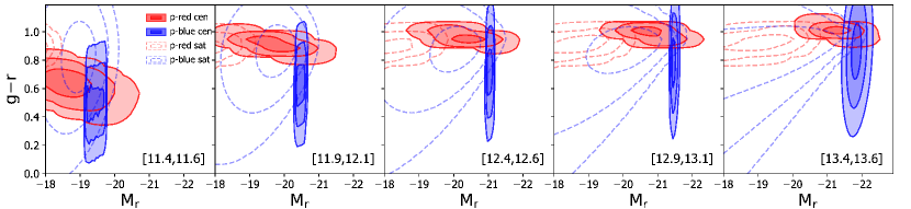
Figure 8: CCMD as a function of halo mass from the best-fitting model. Solid and dotted blue contours are for the pseudo-blue central and satellite galaxy components. Solid and dotted red contours are the same, but for the pseudo-red population. In each component, the contour levels are $\exp(-1/2)$, $\exp(-4/2)$, and $\exp(-9/2)$ times the peak value for this component (corresponding to the inclusion of 39, 86, and 99 per cent of galaxies in the component for a 2D Gaussian distribution). That is, no overall normalisation is applied for the contour levels of different components (see text for detail). The halo mass range in terms of $\log[M_{\rm h}/(h^{-1}{\rm M_{\odot}})]$ is labelled in each panel.

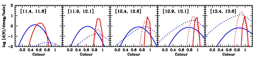
Figure 9: Conditional Colour Function (CCF) as a function of halo mass from the best-fitting model. Solid and dotted blue curves are for the pseudo-blue central and satellite galaxy components. Solid and dotted red curves are the same, but for the pseudo-red population. The CCF of each component is computed for galaxies more luminous than $M_{\rm r}=-18$. The halo mass range in terms of $\log[M_{\rm h}/(h^{-1}{\rm M_{\odot}})]$ is labelled in each panel.

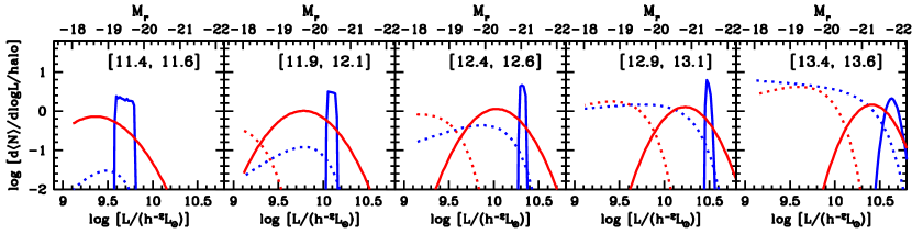
Figure 10: CLF as a function of halo mass from the best-fitting model. Solid and dotted blue curves are for the pseudo-blue central and satellite galaxy components. Solid and dotted red curves are the same, but for the pseudo-red population. The halo mass range in terms of $\log[M_{\rm h}/(h^{-1}{\rm M_{\odot}})]$ is labelled in each panel.

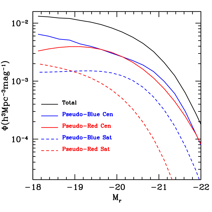
Figure 11: Decomposition of galaxy LF into model components. The LF from the best-fitting model is shown as the thick black curve, which is decomposed into contributions from the pseudo-blue central (thin solid blue) and satellite (thin dashed blue) components and the pseudo-red central (thin solid red) and satellite (thin dashed red) components.

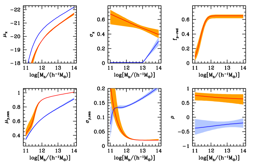
Figure 12: CCMD quantities as a function of halo mass for central galaxies. From left to right and top to bottom, the panels show the halo mass dependence of the mean magnitude, the standard deviation of magnitude, the fraction of pseudo-red central galaxies, the mean colour, the standard deviation of colour, and the correlation coefficient between colour and magnitude (see § 3.1 for physical meanings or definitions of these parameters). Blue and red curves are for pseudo-blue and pseudo-red central galaxies from the best-fitting CCMD model, respectively. The shaded region around each curve represents the 1$\sigma$ range determined from the MCMC chain.

Figure 13: CCMD quantities for satellite galaxies. From left to right, the top panels show the halo mass dependence of the normalisation, the characteristic magnitude, the faint-end slope of the satellite CLF, and the bottom panels show the luminosity-dependent mean colour and standard deviation of the colour for satellite galaxies (see § 3.2 for physical meanings or definitions of these parameters). Light blue and orange curves are for pseudo-blue and pseudo-red satellite galaxies from the best-fitting CCMD model, respectively. The shaded region around each curve represents the 1$\sigma$ range determined from the MCMC chain.

After discussing the reasonable fits to the projected 2PCFs and colour-magnitude distributions of galaxies from the CCMD model, we turn to the CCMD model itself and present the constraints on CCMD parameters and relations.

Fig. 8 shows the colour-magnitude distributions of galaxies in haloes of different masses from the best-fitting model, which demonstrates the CCMD model’s spirit of de-projecting the global CMD along the halo mass axis. In each panel, the two sets of solid (dotted) contours are the distributions of the pseudo-blue and pseudo-red central (satellite) galaxies. As mentioned in § 3, the division of pseudo-blue and pseudo-red galaxies are motivated by the bimodal colour distribution, which can be approximately described as the superposition of two Gaussian components at fixed luminosity. Therefore the pseudo-blue and pseudo-red components do not need to have distinct colours and they can overlap in certain colour ranges.

For each pseudo-colour population, central galaxies (solid contours) appear to be more luminous than satellite galaxies (dotted contours), reflecting the luminosity gap phenomenon (e.g. Yang et al., 2008). In low mass haloes (e.g. with mass of a few times $10^{11}h^{-1}{\rm M_{\odot}}$; leftmost panel of Fig. 8), the pseudo-blue and pseudo-red central galaxies overlap largely in colour and to a lesser extent in luminosity. In high mass haloes (above $10^{12}h^{-1}{\rm M_{\odot}}$), on average the pseudo-blue central galaxies are more luminous (about 0.5 magnitude in median luminosity) than the pseudo-red central galaxies, and they are bluer on average as expected (about 0.1–0.3 magnitude, decreasing slightly with increasing halo mass). While the pseudo-blue central galaxies have a smaller spread in luminosity in high mass haloes, the pseudo-red central galaxies have a narrower colour distribution weakly dependent with halo mass above $10^{12}h^{-1}{\rm M_{\odot}}$. In each central component, galaxy colour does not appear to have a strong correlation with luminosity (see more discussions later in this section). Note that in Fig. 8, the contours are drawn for each individual component, and the contour levels from different components are not meant to be compared. Even though there is the pseudo-red (pseudo-blue) central component in low (high) mass haloes, their total occupation fraction is small (see below).

To have a more detailed view on the colour distributions of pseudo populations as a function of halo mass, we project the CCMD in Fig. 8 onto the colour dimension to form the conditional colour distribution (CCF) in Fig. 9 for galaxies more luminous than $M_{\rm r}=-18$. For the central components, both the pseudo-blue and pseudo-red populations have redder mean colour in more massive halo, and the dependence on halo mass becomes weak above $10^{12}h^{-1}{\rm M_{\odot}}$. The CCF for pseudo-red central galaxies is narrow with an almost constant width in haloes above $10^{12}h^{-1}{\rm M_{\odot}}$, while that for the pseudo-blue central galaxies is broad with a increasing width with halo mass (also see the bottom middle panel in Fig. 12). For the satellite components, like the central ones, the colour distribution of the pseudo-red component is much narrower than that of the pseudo-blue one. In haloes above $10^{12}h^{-1}{\rm M_{\odot}}$, the colour distribution of each pseudo-colour component has little change with halo mass and the median colour or the colour at the distribution peak is around $g-r\sim 0.9$. Compared with the central galaxies, the median colour of pseudo-red satellites is redder in low-mass haloes (leftmost panel of Fig. 8, where the pseudo-red satellite population does not show up because of low normalisation) and becomes slightly bluer in high-mass haloes. For the pseudo-blue population, the median colour of satellites is much redder than that of central galaxies, and the difference decreases with increasing halo mass.

In addition, the CCF plot (Fig. 9) allows a comparison of the normalisation amplitudes of the four pseudo-colour components. It can be clearly seen that the number of satellites keeps increasing with increasing halo mass, from negligibly small in low mass haloes (the leftmost panel) to outer-numbering the central galaxies by more than an order of magnitude in high mass haloes (the rightmost panel). In haloes above $10^{12}h^{-1}{\rm M_{\odot}}$, the relative fraction of pseudo-red and pseudo-blue central galaxies does not change much with halo mass (also see the top right panel in Fig. 12). The CCF also suggests the constitution of the colour bimodality. The satellite colour distribution, consisting of a narrow pseudo-red and a diffuse pseudo-blue contribution with similar median colour, does not show a bimodal pattern. In haloes above $10^{12}h^{-1}{\rm M_{\odot}}$, the median colours of pseudo-blue and pseudo-red central galaxies are well separated, forming a bimodal distribution. The colour bimodality shown in observations (Fig. 4) is caused by the superposition of different galaxy components in haloes of different masses. We emphasise that Fig. 9, along with Fig. 4 and Fig. 8, demonstrates that the pseudo-colour components do not represent observational colour components and they can well overlap in colour.

Marginalising the CCMD over colour reduces to the CLF. In Fig. 10, the CLFs for five halo mass ranges are shown, with the decomposition into the four pseudo-colour components. As inferred from Fig. 8, the median luminosity of the pseudo-blue central galaxy population is higher than that of the pseudo-red one and its CLF has a more narrow distribution. Particularly in low mass haloes, the luminosity of the pseudo-blue central galaxies show a tight correlation with halo mass, with the scatter reaching the floor value set by the model (top-middle panel in Fig. 12), and the width here is mainly determined by the size of the halo mass bin. For haloes with the lowest mass in Fig. 10, the luminosity distribution is wider, because of the steep slope in the luminosity-halo mass relation (top-left panel in Fig. 12) around that mass range. For haloes with the highest mass in Fig. 10, the luminosity distribution is also wider, but this mainly reflects the large scatter in luminosity at fixed halo mass (top-middle panel in Fig. 12). The amplitude of satellite CLF for either the pseudo-blue or pseudo-red component increases with increasing halo mass, and that for the pseudo-blue satellites shifts towards the more luminous end. The faint-end of the CLF for the pseudo-blue component becomes steeper at higher halo mass, while the change in the pseudo-red component is relatively weaker. A comparison with the CLF derived from a group catalogue is presented in § 4.4.

In Fig. 11, the global LF is decomposed into contributions from the various model components. Over the luminosity range considered here, central galaxies dominate the contribution to the LF at any given luminosity. The component contributions from pseudo-blue and pseudo-red central galaxies are comparable, except towards the faint end where the component LF from pseudo-blue central galaxies reaches a factor of two higher than that from pseudo-red central galaxies. For the LF contribution from satellites is dominated by pseudo-blue satellites above $M_{\rm r}\sim-19$ and is taken over by pseudo-red satellites towards the faint end. It is worth emphasising that at low halo masses the colours of pseudo-red centrals are only slightly shifted from those of pseudo-blue centrals (Fig. 8), so the comparable contributions of the two components are consistent with the observation that most low mass centrals are blue (Fig. 3). Conversely, the mean colours of the pseudo-blue and pseudo-red satellite populations are similar at high halo mass, so the dominance of the pseudo-blue contribution at the bright end is driven by the tail of pseudo-blue satellites in its broader Gaussian, where these pseudo-blue galaxies are supposed to be classified as red galaxies in observation, indicated by the dashed lines in Fig. 3. The contributions of blue and red galaxies to the luminosity function (as opposed to pseudo-blue and pseudo-red ones here) were shown previously in Fig. 3.

The overall features and trends in the CCMD and CLF can be more clearly understood by expressing the main CCMD quantities (§ 3.1 and § 3.2) as a function of halo mass. In fact, these are the fundamental relations we are ultimately after with the CCMD model. The CCMD relations related to central galaxies are shown in Fig. 12, as a function of halo mass. In each panel, solid curves correspond to the best-fitting model and the shaded regions enclose the central 68.3 per cent distribution. In the top-left panel, the median luminosity of the two pseudo-colour central galaxy populations has a similar dependence on halo mass, an exponential cutoff towards the low mass end and a power-law form towards the high mass end. The power-law index at the high mass end is 0.28 (0.35) for the pseudo-blue (pseudo-red) central galaxies. The offset between the two curves reflects that at fixed halo mass pseudo-blue central galaxies are on average more luminous or at the same $r$-band median luminosity pseudo-red central galaxies reside in more massive haloes. The scatter in the central galaxy luminosity for the pseudo-red galaxies monotonically decreases with increasing halo mass (top-middle panel), reaching about 0.4 mag in haloes of $10^{14}h^{-1}{\rm M_{\odot}}$. For pseudo-blue central galaxy, the luminosity is tightly correlated with halo mass below $10^{13}h^{-1}{\rm M_{\odot}}$ (nearly zero scatter, reaching the floor 0.01 set in our model) and then the scatter increases to become similar as the pseudo-red central galaxies in cluster-size haloes. The fraction of central galaxies being pseudo-red increases from about 10 per cent in $10^{11}h^{-1}{\rm M_{\odot}}$ haloes to about 65 per cent in $10^{12}h^{-1}{\rm M_{\odot}}$ haloes and flattens towards the high mass end. Note that the luminosity-halo mass relations derived here is for pseudo-colour components. These are different from observationally inferred relations by separating galaxies into blue and red populations based on a luminosity dependent colour cut, e.g. the ones in More et al. (2011a) based on satellite kinematics. Predictions for such relations can be computed from the model.

The mean colour of the pseudo-blue central galaxies increases steadily from $\sim$0.35 to $\sim$0.9 over the halo mass range of $10^{11}$–$10^{14}h^{-1}{\rm M_{\odot}}$ (bottom-left panel in Fig. 12). For the pseudo-red central galaxies, the mean colour has a steep rise of $\sim$0.5mag within the range of $10^{11}$–$10^{12}h^{-1}{\rm M_{\odot}}$, and then slowly increases towards higher halo mass ($\sim$0.1mag over two orders of magnitude in halo mass). For the scatter in colour, the two components have different trends (bottom-middle panel) — while that of the pseudo-blue central galaxies keeps increasing, that of the pseudo-red central galaxies has a sharp decrease in haloes of mass from $10^{11}h^{-1}{\rm M_{\odot}}$ to $10^{12}h^{-1}{\rm M_{\odot}}$ and then reaches a plateau of $\sim$0.02mag towards higher halo mass. This narrow colour distribution of pseudo-red central galaxies suggests that they make a large contribution to the tight red sequence. We note that for the pseudo-red central galaxies, the major changes in the colour distribution (i.e. mean and scatter) occur at halo mass $10^{12}h^{-1}{\rm M_{\odot}}$, coinciding with a characteristic mass in many aspects of galaxy formation, such as the transition from cold-mode to hot-mode accretion (e.g. Birnboim & Dekel, 2003; Kereš et al., 2005).

The bottom-right panel of Fig. 12 shows the correlation between the colour and the magnitude of the pseudo-colour central galaxies as a function of halo mass. Interestingly a positive (negative) correlation exists for the pseudo-red (pseudo-blue) components over the halo mass range probed here. It means that in haloes of fixed mass pseudo-red central galaxies appear slightly bluer at higher luminosity (more negative in magnitude), and the opposite for the pseudo-blue central galaxies. In the CCMD plot (Fig.8), given the correlation the orientation angle $\theta$ of the contours with respect to the $x$-axis (magnitude) is determined by $\tan 2\theta=2\rho\sigma_{\rm x}\sigma_{\rm y}/(\sigma_{\rm x}^{2}+\sigma_{\rm y}^{2})$, with $\sigma_{\rm x}$ and $\sigma_{\rm y}$ the scatters in magnitude and colour, respectively. In most cases we are in the regime that one of $\sigma_{\rm x}$ and $\sigma_{\rm y}$ is much larger than the other (middle panels of Fig. 12) and hence we have either $\theta\sim 0$ or $\theta\sim\pi/2$, which explains why the correlation does not show up prominently in Fig. 8.

Fig. 13 shows the CCMD quantities related to the satellite galaxies. The normalisation $\phi_{s}^{\ast}$ of the satellite CLF for the pseudo-red component is higher than that of the pseudo-blue component and the difference reaches a factor of $\sim$5 in cluster-size haloes (top-left panel). The characteristic luminosity $x_{\rm s}^{\ast}$ of the pseudo-red satellites is lower than that of the pseudo-blue ones (top-middle panel), e.g. about 1.2mag in massive haloes. At the faint end, the CLF of the pseudo-red satellites has a shallower slope than the pseudo-blue satellites (top-right panel of Fig. 13). Below $10^{13}h^{-1}{\rm M_{\odot}}$, the faint end slope for the pseudo-red satellites is not well constrained in the model. On average satellites become redder with increasing luminosity, and the dependence is weaker for the pseudo-red component ($\sim$0.1mag in colour over 4 mag in luminosity; bottom-left panel). The scatter in the colour of the pseudo-red satellites show a weak dependence on luminosity, decreasing from 0.05mag to 0.03mag over 4 mag in luminosity. However, the scatter for the pseudo-blue satellites is a relatively steep function of luminosity, reaching a value similar to those of the pseudo-red satellites at the bright end but a few times higher at the faint end.

Finally, for the luminosity gap (the difference between the median luminosity of central galaxies and the characteristic luminosity of satellite galaxies), the best-fitting model gives 0.64mag for pseudo-blue galaxies and 1.43mag for pseudo-red galaxies.

4.3 Derived Quantities and Relations

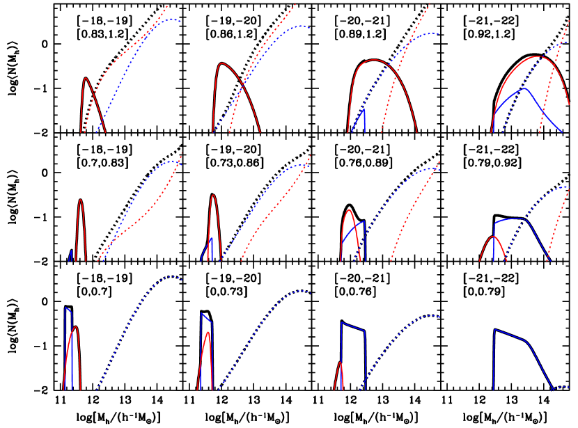
Figure 14: Dependence of the mean occupation function on galaxy colour and luminosity. Each column corresponds to a fixed magnitude bin, with three colour sub-samples of galaxies (blue, green, and red sub-sample from bottom to top), with the magnitude and colour ranges labelled in the panel. In each panel, the thick solid (dotted) black curve is the mean occupation function of central (satellite) galaxies in the given colour and magnitude bin, derived from the best-fitting CCMD model. The thin blue and red curves correspond to those of the pseudo-blue and pseudo-red galaxies (solid for central and dotted for satellite galaxies).

The CCMD modelling connects galaxy colour and luminosity with dark matter haloes. We present a few quantities and relations derived from such a connection.

First, the CCMD model enables us to compute the halo occupation function for a galaxy sample defined by arbitrary cuts in colour and luminosity. In fact, this is how we do the modelling in the first place by figuring out the halo occupation function for each galaxy sample. In Fig. 14, we show the mean halo occupation functions for galaxies in four magnitude bins with each divided into three colour bins (roughly representing the blue, green, and red samples). In each panel, the mean occupation functions are decomposed into the four pseudo-blue/pseudo-red central/satellite components. At each fixed magnitude bin, as the sample becomes redder, the relative contribution from the pseudo-red components increases. The mean occupation function of the pseudo-red central galaxies is smooth, while that of the pseudo-blue central galaxies shows relatively sharp, step-like features, a manifestation of the tight correlation in the model between luminosity of pseudo-blue central galaxies and halo mass in low mass haloes (Fig. 12). The total mean occupation function of central galaxies at a fixed magnitude bin is in the form of a bump, which can usually be approximated by a Gaussian profile. For that of the satellites, it is approximately in a form of power law rolling off towards low mass, except for the bluest sample, which turns over towards the high mass end.

With the mean occupation function of galaxies in each colour and magnitude bin, we can figure out characteristic quantities describing the occupation of galaxies. In Fig. 15, we show an example of such quantities, the median mass of host haloes as a function of galaxy colour and magnitude. The left panel is the median halo mass for all the galaxies in each colour and magnitude bin. In general, the more luminous and redder the galaxy population is, the higher the median halo mass becomes. The majority of blue cloud galaxies have median host halo mass in the range of $10^{11}$–$10^{12}h^{-1}{\rm M_{\odot}}$. The median halo mass for galaxies at the ridge of the red sequence increases from $\sim 10^{12}h^{-1}{\rm M_{\odot}}$ to a few times $10^{13}h^{-1}{\rm M_{\odot}}$ over a range of four magnitudes. At each luminosity, the reddest galaxies appear to have the highest median halo mass.

The middle and right panels in Fig. 15 show the median halo mass for central and satellite galaxies, respectively. The pattern for the central galaxies is similar to that of the total, but the trend along the colour direction becomes weaker. For satellites, the majority of them have median halo mass above $10^{13}h^{-1}{\rm M_{\odot}}$, including those in the blue cloud. At fixed colour and luminosity, satellite galaxies on average reside in more massive haloes than central galaxies. For instance, the faint red central galaxies resides in haloes of a few times $10^{11}h^{-1}{\rm M_{\odot}}$, while faint red satellites are in haloes of a few times $10^{12}h^{-1}{\rm M_{\odot}}$ to a few times $10^{13}h^{-1}{\rm M_{\odot}}$ (e.g. Xu et al., 2016). From the three panels, we can also tell that reddest galaxies are dominated by satellites in relatively massive haloes.

In Fig. 16, we show the fraction of satellites as a function of galaxy colour and magnitude. The gradient is mainly along the colour direction, and redder galaxies are more likely to be satellites. For a detailed inspection, Fig. 17 shows satellite fraction as a function of galaxy colour in several magnitude bins. Zehavi et al. (2011) model the clustering of galaxies in the $-20<M_{\rm r}<-19$ magnitude bin with six fine bins in colour, using a simple HOD model (their fig.20). The satellite fractions derived here are in broad agreement with theirs. The satellite fraction for blue cloud galaxies is generally below 10 per cent. The red galaxies beyond the red sequence ridge are mainly satellites. For faint red galaxies, the satellite fraction is high. For example, for galaxies with $-19<M_{\rm r}<-18$ and $g-r\gtrsim 0.75$, the average satellite fraction is above 50 per cent, increasing with colour. This is consistent with the HOD modelling results in Xu et al. (2016). In the tail of the colour distribution, e.g. redder than $g-r=1$, galaxies are dominated by satellites, especially at the faint end. They are satellites in massive haloes (with median mass of a few times $10^{13}h^{-1}{\rm M_{\odot}}$; right panel of Fig. 15). Pasquali et al. (2010) show that low-stellar-mass satellites in massive haloes are generally older and more metal rich than central galaxies of similar stellar mass. However, such an average trend is not able to explain why those faint satellites are so red. They are even as red as the most luminous galaxies in the CMD here ($M_{\rm r}\sim-22$). It is likely that they have high metallicity, comparable to the massive galaxies. This means that they substantially deviate from the mass-metallicity relation, which is possible if they represent the tail of the heavily stripped galaxies. As shown by Puchwein et al. (2010) with a high-resolution simulation, satellites approaching closely to the cluster centre can be substantially stripped (e.g. with more than 90 per cent of their stellar mass lost; see their fig.16). A metallicity study of those galaxies with spectroscopic observation can help verify the above picture and understand their nature.

We note that, in Fig. 17, there appears to be an upturn in the satellite fraction towards the blue end for galaxy samples with $M_{\rm r}>-19$. One possible reason is that galaxies at the blue end come from the tail of a narrow distribution of pseudo-blue central galaxies and that of a broad distribution of pseudo-blue and pseudo-red satellite galaxies (see Fig. 4). A slight change in the satellite distribution would lead to a large change in the satellite fraction. Also as we approach the tail of the distribution, the results may be sensitive to the functional forms used in the model parameterization. Anyway, at the faint blue end, since there is not much constraining power from the clustering, the uncertainty in the satellite fraction is large and the results are still consistent with a low satellite fraction.

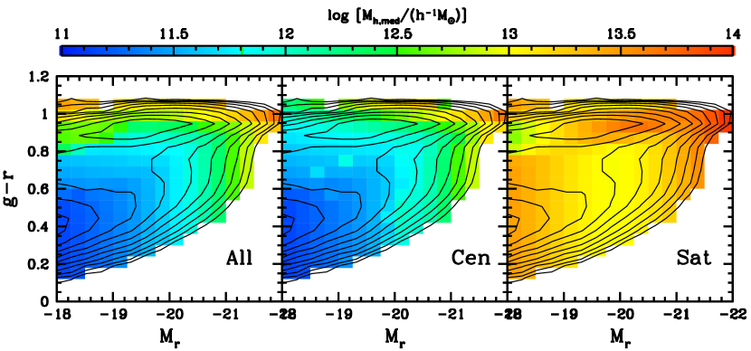
Figure 15: Dependence of median host halo mass on galaxy colour and luminosity from the best-fitting CCMD model. In each panel, colour-coded is the median halo mass $M_{\rm h,med}$ for galaxy samples defined in fine colour and magnitude bins. From left to right, the panels show the median host halo mass distribution for all galaxies, central galaxies, and satellite galaxies, respectively. Contours of galaxy number density are overlaid in each panel to show the bimodality in the overall galaxy population.

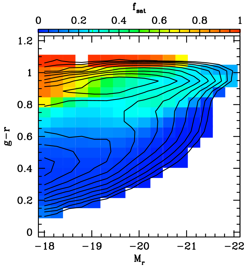
Figure 16: Dependence of satellite fraction on galaxy colour and luminosity from the best-fitting CCMD model. Colour-coded is the satellite fraction $f_{\rm sat}$ for galaxy samples defined in fine colour and magnitude bins. Contours of galaxy number density are overlaid to show the bimodality in the overall galaxy population.

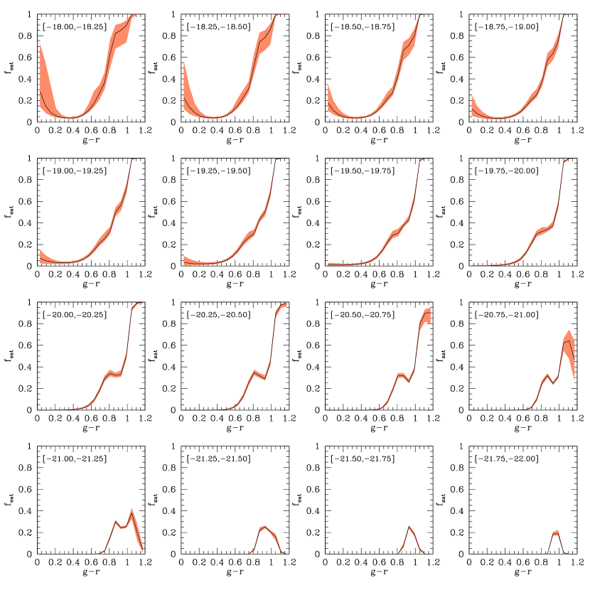
Figure 17: Dependence of satellite fraction on colour for galaxies in different luminosity bins. Galaxy luminosity increases from left to right and top to bottom panels, as labelled in the top-left corner in each panel. In each panel, the solid curve is the satellite fraction from the best-fitting CCMD model and the shaded region indicate the 1$\sigma$ range.

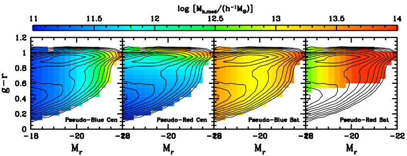
Figure 18: Dependence of median host halo mass on galaxy colour and luminosity for each pseudo-colour model population from the best-fitting CCMD model. In each panel, colour-coded is the median halo mass $M_{\rm h,med}$ for galaxy samples defined in fine colour and magnitude bins. From left to right, the panels show the median host halo mass distribution for pseudo-blue central galaxies, pseudo-red central galaxies, pseudo-blue satellites, and pseudo-red satellites, respectively. Contours of galaxy number density are overlaid in each panel to show the bimodality in the overall galaxy population. Note that the ‘blue cloud’ region in the rightmost panel has no value assigned, as almost no pseudo-red satellites exist there.

Finally, the median halo mass trends seen in Fig. 15 motivate us to study those for each individual pseudo-colour population, as the CCMD model naturally separates them. Such a separation may be more illuminating. Indeed, we find clear and interesting trends. Fig. 18 displays the median halo mass for each of the pseudo-blue/pseudo-red central/satellite components. For pseudo-blue central galaxies (leftmost panel), the median halo mass gradient is along the luminosity direction, with more luminous pseudo-blue central galaxies residing in more massive haloes. In striking contrast, for pseudo-red central galaxies (second to the left panel), the median halo mass gradient is almost completely along the colour direction, with redder pseudo-red galaxies found in more massive haloes. The trends can also be inferred from Fig. 14. The orthogonal dependences of median halo mass on luminosity and colour for the two central galaxy components are remarkable. The results suggest that while halo mass determines the luminosity of pseudo-blue central galaxies, it mainly affects the colour of pseudo-red central galaxies. This seems to indicate that the pseudo-colour populations in the CCMD model have a physical origin, and we leave more discussions on the implications to § 5.

For pseudo-blue satellites (second to right panel in Fig. 18), the median halo mass does not depend on colour and shows only a weak dependence on luminosity. It is about $10^{13}h^{-1}{\rm M_{\odot}}$ for pseudo-blue satellites with luminosity around $L^{\ast}$ and becomes higher for fainter as well as more luminous satellites. The median halo mass for pseudo-red satellites (rightmost panel), on the contrary, shows a clear dependence on luminosity, higher for more luminous satellites. Note that in this panel, no value is assigned in the ‘blue cloud’ region, as there exist almost no pseudo-red satellites. The median halo mass in satellites can also be inferred from Fig. 14 – while the shape of the mean occupation function of the pseudo-blue satellites does not vary significantly with either colour or luminosity, that of the pseudo-red satellites becomes steeper for more luminous satellites. This is consistent with the pseudo-blue satellites being more widely distributed in colour and luminosity across a large halo mass range than the pseudo-red galaxies, as shown in Fig. 8. Similar to the pseudo-colour central components, the distinct difference between the two pseudo-colour satellite components and the clear trend seen with the median halo mass imply that there may be a physical origin of the separation into those components (see more discussions in § 5).

4.4 Comparison of the Derived Galaxy-Halo Relations with Previous Work

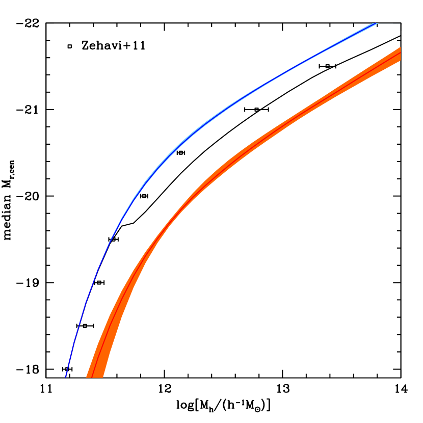
Figure 19: Comparison of the relation between the median central galaxy luminosity and halo mass. The blue and red curves are the relations for pseudo-blue and pseudo-red central galaxies from the best-fitting CCMD model (same as in the top-right panel of Fig. 12), and the black curve is the overall median central galaxy luminosity as a function of halo mass. The data points are from Zehavi et al. (2011), from HOD modelling of the projected 2PCFs of luminosity-threshold samples. See details in the text § 4.4.

Figure 20: Comparison of the relation between the mean halo mass and central galaxy luminosity. The curve is the mean halo mass as a function of central galaxy luminosity from the best-fitting CCMD model. The different sets of data points show the same relation inferred from different probes, including galaxy-galaxy weak lensing (Mandelbaum et al., 2006), satellite kinematics (More et al., 2011b), and CLF modelling of galaxy clustering and galaxy lensing (Cacciato et al., 2009), as labelled in the legend. All vertical error bars, including the boundaries of shaded region, represent the 95 per cent confidence levels, and the horizontal error bars on filled circles indicate the magnitude bins adopted in the galaxy lensing measurements (Mandelbaum et al., 2006) and used in the calculation of the CCMD result. The lensing mass is derived by combining those for the late- and early-type central galaxies in Mandelbaum et al. (2006) and corrected to account for the scatter in the mass-luminosity relation. See the text § 4.4 for detail.

Our CCMD model presents a new way to describe the relation between galaxies and dark matter haloes. It extends the CLF framework by adding a dimension of galaxy colour. The modelling results can be used to derive the CLF or HOD for a galaxy sample defined by cuts in luminosity and colour. We compare the results with the HOD and CLF derived based on previous study. To be consistent with the halo definition used in previous work, we apply the correction mentioned in § 3.3 to convert the halo mass in our results to $M_{\rm 200b}$.

Zehavi et al. (2011) perform HOD modelling of the projected 2PCFs of galaxy samples defined by different luminosity thresholds, using the SDSS DR7 data. For each sample, one of the HOD parameters is $M_{\rm min}$, which is the mass scale of haloes that on average half of them host central galaxies above the luminosity threshold. If at fixed halo mass central galaxy luminosity follows a log-normal distribution (i.e. normal distribution in terms of magnitude) and the median luminosity has a power-law dependence on halo mass, the relation between the threshold luminosity and $M_{\rm min}$ would be just that between the median central galaxy luminosity $\langle M_{\rm r,cen}\rangle$ and halo mass $M_{\rm h}$ (Zheng et al., 2007). Note that here, for a log-normal luminosity distribution, the median luminosity corresponds to the mean magnitude. The data points in Fig. 19 show the $\langle M_{\rm r,cen}\rangle$–$M_{\rm h}$ relation derived in such a way in Zehavi et al. (2011). The relation is also consistent with that inferred from satellite kinematics in More et al. (2009).

The blue (red) curve is the median luminosity of pseudo-blue (pseudo-red) central galaxies as a function of halo mass from the best-fitting CCMD model (same as in the top-left panel of Fig. 12). As the CCMD model has the full distribution of the central galaxy luminosity, which is the superposition of those of pseudo-red and pseudo-blue central galaxies weighted by the relative fraction (top-right panel of Fig. 12), we can obtain the median central galaxy luminosity at each halo mass. The black curve is the $\langle M_{\rm r,cen}\rangle$–$M_{\rm h}$ relation from the best-fitting CCMD model. An inflection feature occurs around $\log[M_{\rm h}/(h^{-1}{\rm M_{\odot}})]=11.6$, the mass scale where pseudo-blue and pseudo-red have equal fraction (top-right panel of Fig. 12). The feature is caused by the narrow luminosity distribution of the pseudo-blue central galaxies (top-middle panel of Fig. 12). With a test of increasing the floor set for the scatter in the pseudo-blue central galaxy luminosity, we find that the inflection feature becomes smoothed, with little effect on other parts of the curve. We note that this inflection will also go away if we use the mean luminosity. While the curve follows well the overall trend seen in Zehavi et al. (2011), it does not exactly match the points at the low mass end. This is not surprising, as the distribution of central galaxy luminosity is not a single log-normal distribution and the relation between median central luminosity and halo mass is not a pure power law. That is, the two conditions to interpret the relation between threshold luminosity and $M_{\rm min}$ as the $\langle M_{\rm r,cen}\rangle$–$M_{\rm h}$ relation in Zehavi et al. (2011) are not satisfied in the CCMD model. From the view point of the CCMD model, the central galaxy luminosity distribution from the contributions of the pseudo-blue and pseudo-red population does not follow a single log-normal distribution, and the commonly adopted form of the central galaxy mean occupation function for luminosity-threshold samples (e.g. Zheng et al., 2005, 2007; Zehavi et al., 2011) should be only treated as a good approximation. The comparison here between the HOD and CCMD modelling results is not exact, but the agreement is reasonable anyway.

The relation between central galaxy luminosity and halo mass can also be expressed in terms of mean halo mass as a function of galaxy luminosity, i.e. the $\langle M_{\rm h}\rangle$–$M_{\rm r,cen}$ relation. In Fig. 20, we conduct a comparison between the relation from the best-fitting CCMD model with those yielded from various other methods, which include galaxy-galaxy weak lensing, satellite kinematics, and CLF modelling of galaxy clustering and weak lensing. Mandelbaum et al. (2006) construct luminosity bin SDSS galaxy samples and perform weak lensing measurements to infer the mean halo mass of early- and late-type central galaxies, respectively. We compute the mean halo mass for all central galaxies based on those for early- and late-type galaxies and their relative fraction (see table 4 and table 2 in Mandelbaum et al. 2006). The lensing measurement result is plotted as the filled circles with vertical error bars marking the 95 per cent confidence level and horizontal error bars indicating the magnitude bins. Note that to convert from the measured excess surface density of mass to mean halo mass, there are additional corrections to account for the halo mass distribution and the scatter in the $M_{\rm h}$–$M_{\rm r,cen}$ relation (Mandelbaum et al., 2005). In Mandelbaum et al. (2006), the result has been corrected, assuming no scatter in the $M_{\rm h}$–$M_{\rm r,cen}$ relation. To be more realistic, here we make a further correction to include the effect of the scatter using a model considered in Mandelbaum et al. (2005) (see their table 1). In detail, with respect to the mean halo mass in Mandelbaum et al. (2006), we add upward corrections of 0 dex, 0.08 dex, 0.15 dex, and 0.14 dex in halo mass for $M_{\rm r}$ magnitude bins [-19,-18], [-20,-19], [-21,-20], and bins with $M_{\rm r}$ more luminous than -21, respectively. The solid curve is the result calculated from the best-fitting CCMD model with the same magnitude bins as in Mandelbaum et al. (2006), which shows an excellent agreement with that inferred from galaxy lensing. For the most luminous bin, the lensing result is slightly lower than the CCMD result, which may be related to the details in modelling the scatter in the $M_{\rm h}$–$M_{\rm r,cen}$ relation and the slightly different cosmological model adopted in Mandelbaum et al. (2006) for modelling the lensing signal. A more direct comparison would be between the excess surface density predicted by the CCMD model and the lensing measurement, which we reserve for future work.

The shaded region in Fig. 20 represents the constraints (95 per cent confidence level) on the $\langle M_{\rm h}\rangle$–$M_{\rm r,cen}$ relation from satellite kinematics in More et al. (2011b). While the constraints are consistent with the CCMD result, the mean halo mass inferred from satellite kinematics is systematically lower (by about 0.2 dex). The reason is not clear, and it is possibly related to some additional effects from satellite velocity bias (e.g. Guo et al., 2015) and the misidentification of a small fraction of central galaxies as satellites. The open squares show the $\langle M_{\rm h}\rangle$–$M_{\rm r,cen}$ relation derived from CLF modelling of galaxy clustering and lensing measurements by Cacciato et al. (2009), which is presented in More et al. (2011b). As the CLF modelling in Cacciato et al. (2009) makes use of the information from the group catalogue (e.g. Yang et al., 2007), the $\langle M_{\rm h}\rangle$–$M_{\rm r,cen}$ relation is almost identical to that from the group catalogue (see More et al., 2011b, fig.10). The mean halo mass from Cacciato et al. (2009) is also systematically lower than the CCMD result, especially for faint galaxies in low mass haloes (e.g. below $\log[\langle M_{\rm h}\rangle/(h^{-1}{\rm M_{\odot}})]\sim 13$). The discrepancy may be related to the underestimation of the halo mass from the group catalogue for haloes hosting blue central galaxies (Lin et al. 2016 and discussions below).

Figure 21: Comparison between the CLF from a group catalogue and that from the best-fitting CCMD model. The halo mass range in terms of $\log[M_{\rm h}/(h^{-1}{\rm M_{\odot}})]$ is labelled in each panel. The circles and squares are the CLFs of central and satellite galaxies from the SDSS DR7 group catalogue, constructed in the same way as in Yang et al. (2008). The error bars are estimated based on 10 jackknife samples. The solid and dotted curves are those from the best-fitting CCMD model. The differences between group-based CLF and CCMD-derived CLF are related to the way of assigning halo mass to groups in the group catalogue. See the text § 4.4 for details.

As the CCMD can be readily inferred with a group catalogue, it is interesting to compare our CCMD modelling results with those from a group catalogue. In particular, this potentially allows the comparison of the full distribution of galaxy luminosity and colour. For such a purpose, we make use of the group catalogue based on the SDSS DR7 data and constructed in the same way as in Yang et al. (2008), who used the DR4 galaxy sample. For groups in a given halo mass bin, the CLF is computed, separating into contributions from central and satellite galaxies. To account for the effect of flux limit for galaxies and the completeness of groups, at each luminosity bin, the average number of galaxies per halo is computed with groups in the volume where both galaxies down to that luminosity and groups in the given halo mass bin are complete. Fig. 21 shows the CLFs from the group catalogue in three halo mass bins, in comparison with those from our best-fitting CCMD model.

For the central galaxies, the CLF from the group catalogue shows a clear double-peak profile, similar to the superposition of two Gaussian profiles (in magnitude). This is exactly in line with the CCMD model, where the central galaxies are composed of the pseudo-blue and pseudo-red populations, each with a Gaussian distribution. In the group-based central CLF, the component with the blue peak has a much narrower distribution than the one with the red peak, meaning that the blue component has a tighter correlation between central galaxy luminosity and halo mass. This is again consistent with the constraints from the CCMD model. However, quantitatively there are clear differences between the group-based CLF (open circles) and the CCMD modelling result (solid curves). The group-based central CLF is more concentrated in luminosity, the peak positions shift with respect to the CCMD model, and the relative contribution of the two components may not agree perfectly with the CCMD model.

The differences can be largely explained by the way halo masses are assigned to the groups. In the group catalogue we use, (apparent) halo mass is determined from the total $r$-band galaxy luminosity (down to $M_{\rm r}=-19.5$) of each group, i.e. through matching the abundances of groups ranked by total luminosity and that of haloes ranked by halo mass. To have a conceptual understanding, suppose that we work in the regime where the total galaxy luminosity of each halo is dominated by the central galaxy (approximately the case for haloes below $\sim 10^{12.5}h^{-1}{\rm M_{\odot}}$). Central galaxy luminosity is then mapped directly onto halo mass. The scatter in central galaxy luminosity in groups of a given halo mass bin simply reflects the size of the mass bin. The intrinsic scatter of central galaxy luminosity at fixed halo mass does not show up in the CLF, which leads to the narrower profile of the group-based central galaxy CLF. Such abundance matching also shifts the median galaxy luminosity and halo mass relation, resulting in the apparent offset of the CLF profile at a given halo mass. By performing a test of the effect of group finding on the conditional stellar mass function (CSMF), Reddick et al. (2013) find that the central CSMF from the group catalogue has a reduced width and shows a peak offset (see their fig.20, squares versus diamonds), in line with our simple analysis. In addition, the halo mass in the group catalogue can be different from the truth and the difference depends on the type of central galaxies. For example, through galaxy lensing measurements, Lin et al. (2016) show that the halo masses of groups of the same apparent halo mass (around $10^{12}h^{-1}{\rm M_{\odot}}$) in the Yang et al. (2007) group catalogue can differ by a factor of 1.9–3.4, with higher masses for those hosting central galaxies of early type or low specific star formation rate (see their fig.1 and fig.2). Such a mass difference is quite consistent with that between the halo masses of the pseudo-blue and pseudo-red central galaxies of the same median luminosity in the CCMD model (top-left panel of Fig. 12). The difference between the apparent halo mass in the group catalogue and the true halo mass can also cause the shift in the peaks of the central galaxy CLF and affect the relative fraction of the red and blue components.

In Fig. 21, the group-based satellite CLF (squares) and that from the CCMD model (black dotted curve) appear to have a better agreement than the central CLFs. The big difference is that the group-based satellite CLF has a steeper cutoff at the high luminosity end than that from the CCMD model. This in fact can be explained in the same way as why the group-based central galaxy CLF is narrower – with the apparent halo mass largely determined by the central galaxy luminosity by ignoring the scatter between luminosity and halo mass, the luminosity gap between the central galaxy and satellites is enhanced. This phenomenon also shows up in the test of halo finding effect in Reddick et al. (2013), as seen in their fig.20 (also see Campbell et al. 2015). In reality, even if the luminosity gap is independent of central galaxy luminosity, the intrinsic scatter in central galaxy luminosity can lead to a much softer high-luminosity cutoff in the average satellite CLF, i.e. a smearing effect. Towards the faint end, the group-based satellite CLF and the CCMD one show a remarkable agreement. We speculate that given the relatively shallow profile of the faint end satellite CLF, any smearing effect (e.g. caused by scatter in central galaxy luminosity or by the inaccurate halo mass in the group catalogue) would not change the profile substantially.

With the group catalogue, more comparisons could be done, such as the colour distribution of central and satellite galaxies (e.g. van den Bosch et al., 2008) or even the CCMD. However, from the above CLF comparison, it is clear that any comparison would not be direct and the interpretation of any differences would not be straightforward. Many factors can affect the comparisons, including the group finding algorithm, the purity and completeness of groups, the way halo mass being assigned, and the definitions of central and satellite galaxies. The best way to do the comparisons is to construct a mock galaxy catalogue from our CCMD modelling results and apply the specific group finding code to find groups in the mock (e.g. Campbell et al., 2015). Then with the SDSS groups and the mock ones, we can do direct and fair comparisons on the distribution of galaxy properties (luminosity and colour). The mock catalogue can also help understand and quantify the systematics in finding groups and in using the group catalogue for various studies. We reserve more comparisons and such a full investigation for future work, with the help of CCMD-based mock galaxy catalogues. The importance of fully modelling the redshift-space group identification procedure for HOD-type clustering analysis is emphasised by Sinha et al. (2018).

5 Summary and Discussion

The bimodal distribution in the galaxy CMD is a main observational feature in properties of galaxies. It encodes important information on galaxy formation and evolution. In this paper, we study the luminosity and colour distribution of galaxies by developing a CCMD model and by modelling the luminosity and colour dependent galaxy clustering, which enables us to connect galaxy luminosity and colour with dark matter haloes and to deproject the global galaxy CMD into a halo mass dependent distribution with a decomposition into contributions from central and satellite galaxies. This model, and its calibration against clustering measurements for many finely binned samples of SDSS galaxies, substantially extends our previous studies of the luminosity and colour dependence of the galaxy correlation function (Zehavi et al., 2005a, 2011).

The CCMD parameterization is mainly motivated by the fact that the colour distribution of galaxies at fixed luminosity can be well described by the superposition of two Gaussian components, which guides us to introduce the pseudo-blue and pseudo-red model populations. Each population is further divided into the central and satellite galaxy components. At fixed halo mass, the magnitude and colour of each pseudo-colour central population follows a 2D Gaussian distribution. For satellite galaxies, at fixed halo mass, their luminosity distribution is parameterized as a Schechter-like function and their colour follows a luminosity-dependent Gaussian distribution. The characteristic quantities of the central and satellite CCMD are further parameterized as a function of halo mass, motivated by previous work on HOD and CLF modelling. The quantities include the median and scatter of the central galaxy magnitude and those of the colour and the correlation between central galaxy magnitude and colour for each pseudo-colour central component, and the normalization, faint end slope, and characteristic luminosity of the satellite CLF for each pseudo-colour satellite component. Because of the width of the pseudo-blue and pseudo-red distributions, the two populations can overlap in true colour, sometimes substantially (see Figs. 4 and  8). The CCMD model employs a global parameterization in the sense that it describes the overall distribution of galaxy luminosity and colour as a function of halo mass, not specific to any particular galaxy sample. Given a set of CCMD parameters, the mean occupation function can be readily calculated for a sample of galaxies with any luminosity and colour cuts, and then the clustering statistics of the sample can be computed with the halo population of a cosmological model.

We apply the CCMD formalism to model the abundances and projected 2PCF measurements of galaxy samples defined by fine luminosity and colour bins, constructed from the SDSS DR7 data. The model is able to well reproduce the data, which include the abundances and projected 2PCF measurements of 79 galaxy samples covering the galaxy CMD in the range of $-22<M_{\rm r}<-18$ and $0<g-r<1.2$, with 13 data points per sample. The model seems to have a large number of free parameters, 59 in total. However, the number of parameters of this global CCMD model is in fact much less than that in a model where each sample is parameterized separately, as done in previous work (e.g. 5 parameters per sample). In our application here, each sample only has $\sim 0.7$ parameter on average. The luminosity and colour dependent clustering makes it possible to infer the halo mass dependent CCMD, and the small-scale clustering provides sufficient constraining power to separate the central and satellite components.

The main results from the CCMD modelling of SDSS galaxy clustering include:

• For central galaxies, the CCMDs of the two pseudo-colour populations are distinct and almost orthogonal to each other. At fixed halo mass, the pseudo-blue central galaxies have a narrow luminosity distribution but spread in colour, while the pseudo-red central galaxies have a narrow colour distribution but spread in luminosity. The mean colours of the two components become comparable at halo mass $\sim 10^{11.5}h^{-1}{\rm M_{\odot}}$.

• For each pseudo-colour central component, below halo mass of $\sim 10^{12}h^{-1}{\rm M_{\odot}}$, the median luminosity sharply increases with halo mass. At the high mass end, the dependence approaches a power law with an index of 0.28 (for pseudo-blue galaxies) or 0.35 (for pseudo-red galaxies). At fixed halo mass, pseudo-blue central galaxies are more luminous in $r$-band than pseudo-red ones, by about one (half) magnitude at the low (high) mass end. Or, for pseudo-blue and pseudo-red central galaxies of similar luminosity (in the sense of median luminosity), the latter reside in more massive haloes, with mass about 0.2 (1) dex higher at the faint (luminous) end.

• The fraction of central galaxies in the pseudo-red component increases with halo mass and approaches a plateau of $\sim$65 per cent above $10^{12}h^{-1}{\rm M_{\odot}}$, where the colour distribution of this component also becomes narrow (about 0.02mag in scatter).

• Based on the median mass of the host haloes, for pseudo-blue central galaxies it is the luminosity that strongly correlates with halo mass, more luminous in more massive haloes, while for pseudo-red central galaxies, it is the colour, redder in more massive haloes.

• For satellite galaxies, the dependences of the characteristic luminosity on halo mass of the two pseudo-colour components follow a trend similar to the ones seen in the median central galaxy luminosity, with the difference being much larger (e.g. $\sim 1.5$mag difference in the characteristic luminosity at fixed halo mass). The faint-end slope of the CLF of the pseudo-blue satellites is generally steeper than that of the pseudo-red satellites.

• The pseudo-blue satellite component has a large spread in colour at most luminosities, with a decrease of scatter at the highest luminosities ($M_{\rm r}\lesssim-20.5$). The pseudo-red satellite component has a narrow colour distribution, with the scatter decreasing slowly (from 0.06mag to 0.03mag) with luminosity.

• At low luminosities, roughly $M_{\rm r}\gtrsim-19$, the bimodality of the galaxy CMD is driven largely by the contribution of blue centrals and red satellites. At higher luminosities, the bimodality is driven mainly by the blue and red central galaxy components, with satellites playing a steadily decreasing role.

• For a typical galaxy sample, colour is the strongest indicator of a galaxy’s probability of being a satellite, with luminosity being a secondary factor. The satellite fraction is higher for redder galaxies and higher for fainter ones, and it exceeds 50 per cent for faint red galaxies. The population of extremely red faint satellites likely originates from massive satellites whose stellar content has been heavily reduced by stripping.

• For satellites, the median host halo mass of the pseudo-blue component does not show a strong dependence on colour and luminosity, while that of the pseudo-red component increases with satellite luminosity.

In Zehavi et al. (2005a, 2011), we model the difference in clustering of red and blue galaxies at fixed luminosity as a consequence of the larger satellite fraction of red galaxies. While our analysis here (like many others) confirms this higher satellite fraction, it also shows that the halo masses of red central galaxies are higher than those of blue centrals at fixed luminosity (conclusion 2 above). Galaxy-galaxy weak lensing measurements provide direct evidence for this mass difference (Zu & Mandelbaum, 2016, 2018), which is derived here from clustering alone.

While the separation into pseudo-blue and pseudo-red populations in the model is initially phenomenological, motivated by the bimodal distribution of galaxies, the modelling results do show distinct differences of the two model populations, which indicates that the two pseudo-colour populations have a physical origin. We speculate that the pseudo-blue central galaxies are dominated by galaxies with episodes of star formation during the past 2–3 Gyrs. The large scatter in colour may reflect the differences in the time and duration of the star formation as well as effects of dust and metallicity. After the star formation shuts down, the stellar population evolves fast during the first 2–3 Gyrs, becoming fainter and redder, and then its colour evolves more slowly (e.g. Bruzual & Charlot, 2003). This may lead to the pseudo-red central galaxy population, which has a narrow colour distribution. That is, if we start with the pseudo-blue central CCMD, passive evolution alone within 2–3 Gyrs is able to ‘rotate’ it to become close to the pseudo-red CCMD. It may be that the central galaxy CCMD has more than the two above components, but the relatively fast transition makes the two components the dominant modes.

For the pseudo-blue central galaxies, the correlation between luminosity and colour (with fainter galaxies appearing to be bluer) may be a manifestation that some effect of a transitional population (e.g. ‘pseudo-green’ galaxies) has been included. The luminosity of pseudo-blue central galaxies is correlated with halo mass, which may be related to the amount of cold gas available for star formation. For pseudo-red central galaxies, the colour shows a main correlation with halo mass and the luminosity to a less degree, which may be translated from the correlation between halo mass and the time of last episode of star formation and the mass-metallicity relation.

For satellite galaxies, the difference in the luminosity and colour distribution of the two pseudo-colour populations may be related to the dynamical evolution (tidal and ram pressure stripping and strangulation) of the satellites inside the parent haloes. The pseudo-blue satellites may be those falling into the parent halo recently, while pseudo-red satellites have orbited around for a longer time. Hydrodynamic galaxy formation simulations (e.g. Vogelsberger et al., 2014; Schaye et al., 2015) and SAMs (e.g. Guo et al., 2013) can be used to test the existence of the two populations and to better understand their origins, and conversely, our modelling results can be used to test galaxy formation models. We reserve such investigations for future work.

For galaxies more luminous than $M_{\rm r}=-20$, there appears to be a systematic trend in the projected 2PCFs for the bluest galaxy sample, a high clustering amplitude and steep clustering profile on sub-Mpc scales (see Fig. 5). The CCMD model does not capture this trend well. As the signal-to-noise is low for each bluest sample at fixed luminosity bin, we performed a test with a luminous blue galaxy sample over a large range in luminosity, constructed using a tilted cut in the CMD. We find that the above small-scale clustering features persist. This could be a indication that the bluest satellites have a much steeper spatial distribution profile than assumed in our CCMD model. Further investigation with modelling and with galaxy formation models will be useful to better understand the clustering of luminous blue galaxies.

Our CCMD model assumes a specific functional form for the CMD at fixed halo mass: 2D Gaussians for the pseudo-blue and pseudo-red central and satellite populations. Note that this is not exactly true for each satellite component, but the satellite CCMD can be broadly regarded as the superposition of a set of 2D Gaussians. To ensure a globally coherent description with a manageable number of parameters, it assumes particular functional forms for the variation of these 2D Gaussians with halo mass; these forms are motivated by previous observational analyses. We assume the halo mass function and halo clustering of a specific cosmological model, and we assume that the satellite galaxies trace the dark matter distribution within each halo while central galaxies reside at the halo potential minimum. These assumptions could be adjusted without altering the basic principles of the model. The more fundamental physical assumption is that the statistical distributions of galaxy luminosity and galaxy colour depend only on halo mass, not on halo environment or on other halo properties that are correlated with environment. This assumption underpins our predictions of galaxy clustering in the two-halo regime, as we populate haloes using only their masses, and internal profiles (for satellites).

It has been established from $N$-body simulations that the clustering of haloes depends not only on halo mass, but also on halo assembly history (e.g. Sheth & Tormen, 2004; Gao et al., 2005; Wechsler et al., 2006; Harker et al., 2006; Zhu et al., 2006; Jing et al., 2007; Zhu et al., 2006; Li et al., 2008; Salcedo et al., 2018; Xu & Zheng, 2018), which is termed as halo assembly bias. If galaxy properties closely tie to halo formation history and environment, the inherited assembly bias from the host haloes would break the above assumption. If such a galaxy assembly bias effect exists and is strong, it would affect the clustering modelling and introduce systematics in cosmological constraints (e.g. Zentner et al., 2014, 2016). Galaxy assembly bias has been searched for in galaxy formation simulations and models, and no definite conclusion has been reached. SAMs predict significant galaxy assembly bias effects (e.g. on the HOD, CLF and clustering of low-mass galaxies; Zhu et al. 2006; Croton et al. 2007; Zehavi et al. 2018). While the HODs in the hydrodynamic simulations studied in Berlind et al. (2003) and Mehta (2014) show little dependence on halo environment, galaxy assembly bias in the EAGLE simulation (Schaye et al., 2015) leads to $\sim$25% effect on the galaxy 2PCFs at large scales (Chaves-Montero et al., 2016). The different results from different models/simulations suggest that galaxy assembly bias in current galaxy formation models depends on the implementation details of star formation and feedback. Conversely, if galaxy assembly bias can be inferred from observation, it would test such aspects in galaxy formation theories.

The search for assembly bias effect in galaxy survey data has not reached a definite conclusion, either. The difficulty in detecting halo and galaxy assembly bias from observation lies in determining halo mass and finding the appropriate galaxy property as assembly proxy. Using an SDSS galaxy group catalog, Yang et al. (2006) claim the detection of assembly bias (see also Wang et al. 2013; Lacerna et al. 2014), where halo mass is estimated in a similar way as the abundance matching technique (e.g. Conroy et al., 2006) and the star formation rate in the central galaxy is used as a proxy for halo age. Also with an SDSS galaxy group catalog, Berlind et al. (2006) show a detection of assembly bias, but with a trend opposite to that in Yang et al. (2006). A key source of uncertainty in these studies is that groups with blue and red central galaxies may have different halo mass at fixed total luminosity, as suggested by our results here and by the galaxy-galaxy weak lensing analysis of Zu & Mandelbaum (2016). Lin et al. (2016) perform a more careful analysis of assembly bias in SDSS central galaxies, aided by galaxy lensing measurements to control the halo mass, and no evidence is found for assembly bias. This lack of detection suggests that the correlation, if any, between the chosen galaxy assembly indicator (e.g. star formation rate or galaxy formation time) and halo formation history may not be tight. Analyses of the luminosity dependent galaxy clustering in the SDSS show no evidence of galaxy assembly bias for luminous samples and marginal evidence for faint samples (e.g. Vakili & Hahn, 2016; Zentner et al., 2016). Recently, strong assembly bias effect is claimed to be detected with massive clusters, when clusters are split into subsamples based on the average projected distance between satellite and central galaxies (Miyatake et al., 2016; More et al., 2016; Baxter et al., 2016), and the unexpectedly large halo assembly bias was attributed to be possibly related to the nature of dark matter. However, the re-analysis of Zu et al. (2017) with a better control of projection effects shows no evidence of assembly bias.

Our CCMD modelling results can help constrain galaxy assembly bias effect and we plan to work on such a study. We can construct a mock galaxy catalogue by populating haloes in $N$-body simulations according to the best-fitting CCMD model (and/or a series of mocks from a set of models to probe the uncertainties). This catalogue with galaxy luminosity and colour information would be an ideal control sample, free of galaxy assembly bias effect but reproducing the distributions of galaxy luminosity and colour and the luminosity and colour dependent clustering of SDSS galaxies. With such a control sample, we plan to measure and compare a variety of environment dependent statistics in both the mock catalogue and in real data. Potential galaxy assembly signatures will be revealed by the difference between the two types of measurements. The mock catalogue will also have many other applications, such as helping derive accurate covariance matrices for galaxy clustering and testing galaxy survey designs. Another application is to aid the comparison between our CCMD modelling results and those from group catalogues, by applying group finding algorithm to the mock galaxy catalogue. This will in turn help understand systematics in various applications based on the group catalogue (e.g. Campbell et al., 2015), including those in constraining assembly bias and those mentioned in § 4.4. The mock catalogue also makes it easy to compute cross-correlation functions between different samples, which will allow various tests.

In this paper, the CCMD model is constrained by galaxy number densities and galaxy auto-correlation functions. The results can be tested with other clustering statistics, e.g. the cross-correlation functions between individual colour sub-samples at a fixed magnitude bin and the full sample in the magnitude bin. The cross-correlation measurements can be compared with CCMD model predictions based on the method similar to that presented in § 3.3 or mock catalogues for a consistency check. A more effective use of the cross-correlation functions is to include them directly in constraining the model. The cross-correlations with the full sample at fixed magnitude bin not only have reduced shot noise but also encode information about galaxy pairs made of galaxies from colour sub-samples, both of which help tighten the model constraints. Similarly galaxy lensing measurements for samples defined by fine bins of luminosity and colour across the galaxy CMD can also serve as a consistency check or a way to tighten model constraints, especially on the halo mass scales and satellite fractions of different samples (e.g. Leauthaud et al., 2011; Leauthaud et al., 2012; Tinker et al., 2013). The model can be further applied to and constrained by statistics like redshift-space clustering and higher-order clustering, which can bring in additional information, such as the relation between galaxy kinematics and luminosity/colour.

The CCMD modelling results can be compared to the galaxy-halo connections inferred from other methods. The SHAM method (e.g. Conroy et al., 2006) maps galaxy luminosity or stellar mass onto halo properties through matching the cumulative galaxy LF or stellar mass function with the cumulative abundance of haloes/sub-haloes (e.g. in terms of mass or circular velocity). Our result shows that the mapping from luminosity to halo mass needs to account for the dependence on galaxy colour (Fig. 12). Using the estimate of stellar mass from galaxy luminosity and colour with the method in Bell et al. (2003), we find that this remains true for connecting galaxy stellar mass to halo mass (see also Rodríguez-Puebla et al. 2015; Zu & Mandelbaum 2016, 2018). Whether the conclusion holds for other halo properties (e.g. circular velocity) is yet to be tested. The extended ‘age-matching’ method (Hearin & Watson, 2013) assigns galaxy colour based on halo/sub-halo formation time. By construction, the method reproduces the galaxy CMD. Although it reasonably reproduces the colour-dependent galaxy 2PCFs for galaxy samples divided into red and blue sub-samples, its performance on modelling the clustering of galaxies in fine colour bins remains to be tested and compared with the CCMD model. The CCMD modelling results can inform the range of validity of the ‘age-matching’ method. Last but not least, the CCMD model that reproduces the luminosity and colour dependent clustering can be used to test against predictions from galaxy formation models, including both hydrodynamic simulations and SAMs. The differences between the empirically constrained CCMD and galaxy formation model predictions can provide insight about physical processes in galaxy formation and help improve galaxy formation models.

The CCMD model presented in this paper studies galaxies in term of the directly observed galaxy properties, luminosity and colour. In principle, the formalism can be generalised to study galaxy samples defined by inferred quantities, such as the stellar mass and star formation rate, the two quantities more physically related to galaxy formation and evolution. Or, as an intermediate step, one can construct and model galaxy samples defined by galaxy stellar mass and colour. Many analyses in this paper and proposed above can be equally done with such modelling, which will yield further insights into understanding galaxy formation and evolution. Furthermore, results of CCMD-like modelling of galaxy clustering at different redshifts can be used to learn about the evolution of galaxies in the CMD and the buildup and evolution of the bimodality.

Appendix A Galaxy Samples

Table 1 lists the sample information for the 79 galaxy samples used in our CCMD modelling, defined by fine bins in colour and luminosity. The samples are constructed following the steps laid out in § 2.1. All the samples are volume-limited, and the samples of the same magnitude cuts (thus the same $z_{\rm min}$ and $z_{\rm max}$) have the same volume. At each magnitude bin, the division into colour sub-samples depends on the galaxy number within the volume, balancing between reaching reasonable signal-to-noise ratios of clustering measurements and capturing fine features along the colour direction.

Table 1: The 79 volume-limited galaxy samples defined by fine bins in magnitude and colour. The first and second columns are the luminosity and colour ranges of the galaxy samples, respectively. The maximum redshift of each sample is listed in the third column with the same minimum redshift $z_{\rm min}=0.02$ adopted for all the samples. For each sample, the fourth and fifth columns are the number of galaxies in the specific sample volume and its number density in unit of $h^{3}{\rm Mpc^{-3}}$.

$M_{\rm r}$ (mag)	${\rm g-r}$ (mag)	$z_{\rm max}$	$N_{\rm gal}$	$n_{\rm gal}(h^{3}{\rm Mpc^{-3}})$
[-18.00, -18.25]	[0.00,0.44]	0.04257	1667	1.28E-03
	[0.44,0.65]	0.04257	1556	1.19E-03
	[0.65,1.20]	0.04257	1651	1.26E-03
[-18.25, -18.50]	[0.00,0.46]	0.04759	2145	1.14E-03
	[0.46,0.71]	0.04759	2202	1.17E-03
	[0.71,1.20]	0.04759	2188	1.16E-03
[-18.50, -18.75]	[0.00,0.49]	0.05318	2826	1.06E-03
	[0.49,0.75]	0.05318	2873	1.08E-03
	[0.75,1.20]	0.05318	2847	1.06E-03
[-18.75, -19.00]	[0.00,0.52]	0.05941	3635	9.64E-04
	[0.52,0.79]	0.05941	3456	9.17E-04
	[0.79,1.20]	0.05941	3558	9.43E-04
[-19.00, -19.25]	[0.00,0.55]	0.06634	4800	9.08E-04
	[0.55,0.83]	0.06634	4714	8.92E-04
	[0.83,1.20]	0.06634	4820	9.12E-04
[-19.25, -19.50]	[0.00,0.59]	0.07403	6485	8.82E-04
	[0.59,0.86]	0.07403	6461	8.77E-04
	[0.86,1.20]	0.07403	6308	8.56E-04
[-19.50, -19.75]	[0.00,0.53]	0.08258	5036	4.93E-04
	[0.53,0.68]	0.08258	5068	4.97E-04
	[0.68,0.84]	0.08258	4997	4.90E-04
	[0.84,0.92]	0.08258	5172	5.07E-04
	[0.92,1.20]	0.08258	5011	4.91E-04
[-19.75, -20.00]	[0.00,0.53]	0.09207	4920	3.49E-04
	[0.53,0.66]	0.09207	5211	3.70E-04
	[0.66,0.80]	0.09207	5157	3.66E-04
	[0.80,0.89]	0.09207	5013	3.56E-04
	[0.89,0.94]	0.09207	5357	3.80E-04
	[0.94,1.20]	0.09207	4946	3.51E-04

Table 2: continued

The 79 volume-limited galaxy samples defined by fine bins in magnitude and colour. $M_{\rm r}$ (mag) ${\rm g-r}$ (mag) $z_{\rm max}$ $N_{\rm gal}$ $n_{\rm gal}(h^{3}{\rm Mpc^{-3}})$ [-20.00, -20.25] [0.00,0.57] 0.10258 5922 3.05E-04 [0.57,0.69] 0.10258 5407 2.79E-04 [0.69,0.82] 0.10258 5706 2.94E-04 [0.82,0.90] 0.10258 5600 2.89E-04 [0.90,0.95] 0.10258 6613 3.41E-04 [0.95,1.20] 0.10258 5096 2.63E-04 [-20.25, -20.50] [0.00,0.57] 0.11422 5381 2.02E-04 [0.57,0.68] 0.11422 5534 2.08E-04 [0.68,0.79] 0.11422 5667 2.13E-04 [0.79,0.88] 0.11422 5879 2.21E-04 [0.88,0.92] 0.11422 5046 1.90E-04 [0.92,0.96] 0.11422 6329 2.38E-04 [0.96,1.20] 0.11422 4944 1.86E-04 [-20.50, -20.75] [0.00,0.58] 0.12709 5120 1.41E-04 [0.58,0.68] 0.12709 5334 1.47E-04 [0.68,0.77] 0.12709 5032 1.38E-04 [0.77,0.85] 0.12709 5068 1.39E-04 [0.85,0.90] 0.12709 4898 1.35E-04 [0.90,0.94] 0.12709 6635 1.82E-04 [0.94,0.97] 0.12709 5127 1.41E-04 [0.97,1.20] 0.12709 4507 1.24E-04 [-20.75, -21.00] [0.00,0.60] 0.14132 5329 1.08E-04 [0.60,0.70] 0.14132 5295 1.07E-04 [0.70,0.79] 0.14132 5373 1.08E-04 [0.79,0.87] 0.14132 5918 1.19E-04 [0.87,0.91] 0.14132 4886 9.86E-05 [0.91,0.94] 0.14132 5604 1.13E-04 [0.94,0.97] 0.14132 5615 1.13E-04 [0.97,1.20] 0.14132 5150 1.04E-04 [-21.00, -21.25] [0.00,0.64] 0.15702 5465 8.13E-05 [0.64,0.76] 0.15702 6221 9.25E-05 [0.76,0.85] 0.15702 5409 8.04E-05 [0.85,0.91] 0.15702 6135 9.12E-05 [0.91,0.94] 0.15702 5315 7.90E-05 [0.94,0.97] 0.15702 5631 8.37E-05 [0.97,1.20] 0.15702 5687 8.46E-05 [-21.25, -21.50] [0.00,0.69] 0.17434 5599 6.16E-05 [0.69,0.82] 0.17434 5605 6.17E-05 [0.82,0.90] 0.17434 5316 5.85E-05 [0.90,0.94] 0.17434 5651 6.22E-05 [0.94,0.97] 0.17434 5387 5.93E-05 [0.97,1.20] 0.17434 5880 6.47E-05 [-21.50, -21.75] [0.00,0.75] 0.19342 5308 4.34E-05 [0.75,0.89] 0.19342 5114 4.18E-05 [0.89,0.94] 0.19342 5045 4.12E-05 [0.94,0.98] 0.19342 5891 4.82E-05 [0.98,1.20] 0.19342 4642 3.79E-05 [-21.75, -22.00] [0.00,0.90] 0.21441 5929 3.61E-05 [0.90,0.97] 0.21441 6099 3.71E-05 [0.97,1.20] 0.21441 5403 3.29E-05

Appendix B Tests with Parameter Constraints

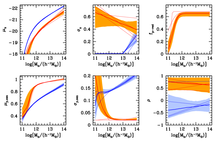
Figure 22: CCMD quantities (defined in § 3.1) as a function of halo mass for central galaxies. Similar to Fig.12, but with the shaded regions corresponding to 2$\sigma$ ranges and with thin curves added from four perturbed runs (see the text in Appendix B).

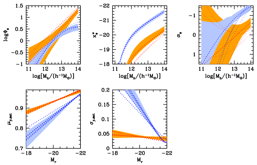
Figure 23: CCMD quantities (defined in § 3.2) as a function of halo mass for satellite galaxies. Similar to Fig.13, but with the shaded regions corresponding to 2$\sigma$ ranges and with thin curves added from four perturbed runs (see the text).

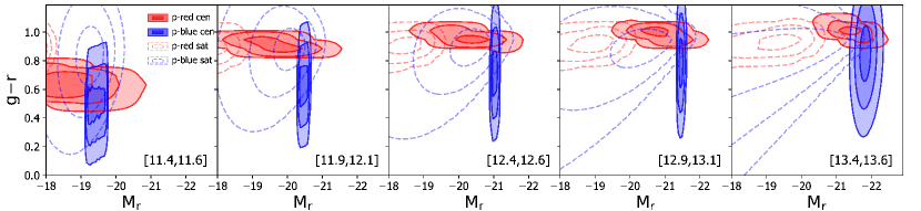
Figure 24: Similar to Fig.8 but for the parameter set with a flat $\sigma_{\rm y,cen}-M_{\rm h}$ relation shown in the bottom-middle panel in Fig. 22.

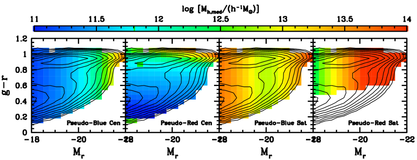
Figure 25: Similar to Fig.18 but for the parameter set with flat $\sigma_{\rm y,cen}-M_{\rm h}$ relation shown in the bottom-middle panel in Fig. 22.

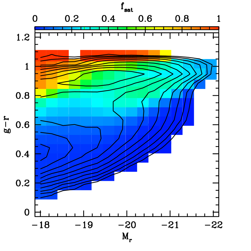
Figure 26: Similar to Fig. 16 but for the parameter set with flat $\sigma_{\rm y,cen}-M_{\rm h}$ relation shown in the bottom-middle panel in Fig. 22.

The CCMD model is characterised by 59 parameters (§ 3.1 and § 3.2). To help explore such a high-dimensional parameter space, we first run a set of test MCMC chains of length around 500,000 with different starting positions. Based on the results of the test runs, we further apply the Gauss-Newton method to search for minima in the $\chi^{2}$ surface. We then use the position with the minimum $\chi^{2}$ as the starting point to the run the chain of length $10^{8}$, and the results in the main text are based on such a run. The CCMD parameterization follows natural forms of the relations between galaxy properties and halo mass, which is not optimised in any way to reduce parameter degeneracies. In terms of the results, it is the physical relations (like those in Fig. 8, Fig.12, and Fig. 13) instead of the relations among parameters themselves that are of interest. Also the derived quantities and trends, like those in Fig. 15 and Fig. 16, provide useful and meaningful information for the model constraints.

There are possibilities that the default results we adopt in the main text come from a local minimum or that there are locations in the parameter space with results highly degenerate with the default ones. To see how such possibilities affect the derived relations and trends, we perform tests by perturbing the parameters to run additional MCMC chains. We start from the positions of the best-fitting model in the main text and randomly perturb each parameter by -5$\sigma$, 0, and 5$\sigma$, where the value of 1-$\sigma$ range of the parameter is determined from the local curvature of the $\chi^{2}$ surface along the parameter direction. We then randomly choose different combinations of the perturbed parameters to start test MCMC runs, each with length 500,000.

In Fig. 22 and Fig. 23, the thin curves show the relations between CCMD properties and halo mass from best-fitting models resulting from 4 such perturbed runs, all of which have $\chi^{2}\sim 950$. The shaded regions represent the 2-$\sigma$ range in the default model. In most ranges, the curves from the perturbed runs fall into the 2-$\sigma$ range. However, there are a few noticeable deviations. For example, in the $\sigma_{\rm y,cen}-M_{\rm h}$ panel of Fig. 22, there are curves corresponding to much narrow colour distribution for the pseudo-red central galaxies in low mass haloes, while in the $f_{\textrm{p-red}}-M_{\rm h}$ panel there is a case with sharp increase in $f_{\textrm{p-red}}$ around $\log[M_{\rm h}/(h^{-1}{\rm M_{\odot}})]=11.2$ to the asymptotic value. Since at the lowest luminosity ($M_{\rm r}=-18$), the mass of the host haloes of the pseudo-red central galaxies is around $\log[M_{\rm h}/(h^{-1}{\rm M_{\odot}})]=11.4$ (top-left panel), the mass range of the above large deviations is where the model is poorly constrained. Therefore, the deviations suggest model degeneracies in the weakly constrained regions of the parameter space with the galaxy samples used in the modelling.

To see how the results are affected, we show the CCMD and derived relations and trends from a parameter set with $\sigma_{\rm y,cen}-M_{\rm h}$ relation being almost a flat curve in the bottom-middle panel of Fig. 22. Its CCMD (Fig. 24) is almost the same as the default model (Fig. 8), in terms of the trends and orientations in the four pseudo-colour components. The main difference is in the panel corresponding to the lowest mass bin, where the pseudo-red central component becomes slightly tighter in the colour direction and less tilted. The median halo mass (Fig. 25) for the pseudo-colour components and the luminosity/colour dependent satellite fraction (Fig. 26) are quite similar to those seen in Fig. 18 and Fig. 16, with the median halo mass of pseudo-blue central galaxies being slightly lower. We also apply the same analyses to the parameter set with the sharply increasing curve in the $f_{\textrm{p-red}}-M_{\rm h}$ panel of Fig. 22 and find a similar result. For this model, the lower fraction of pseudo-blue central galaxies in the mass range of $\log[M_{\rm h}/(h^{-1}{\rm M_{\odot}})]\sim$11.2-12.0 is compensated by putting more pseudo-blue satellites into those haloes, while approximately conserving the abundances and clustering of blue galaxies. Note that the constraining power from galaxy clustering of the faint, blue samples are especially limited, and the abundances is more likely to be the driving force in the model fitting because of the small uncertainties. Larger survey for the faint samples would improve the model constraints.

Our tests show that there are regions in the parameter space that correspond to degenerate solutions, with the CCMD relations and derived quantities/trends similar to those in our default models. On the one hand, this is reassuring as the main results and conclusions of the paper hold. On the other hand, it implies that a full exploration of the high-dimensional parameter space is difficult. We therefore take a practical view of our best-fitting model. It works in reproducing the colour/luminosity dependent clustering and the abundance distribution in the galaxy CMD, and its validity can be further tested with other statistics (e.g. higher order clustering and galaxy lensing measurements). For some applications with the mock galaxy catalogues constructed based on the modelling results (as discussed in § 5), it would be necessary to account for the systematic uncertainties from the above tests for more complete investigations.

References

- Abazajian et al. (2009) Abazajian K. N., et al., 2009, ApJS, 182, 543
- Adelman-McCarthy et al. (2008) Adelman-McCarthy J. K., et al., 2008, ApJS, 175, 297
- Baldry et al. (2004) Baldry I. K., Glazebrook K., Brinkmann J., Ivezić Ž., Lupton R. H., Nichol R. C., Szalay A. S., 2004, ApJ, 600, 681
- Baxter et al. (2016) Baxter E. J., Rozo E., Jain B., Rykoff E., Wechsler R. H., 2016, MNRAS, 463, 205
- Behroozi et al. (2013) Behroozi P. S., Wechsler R. H., Wu H.-Y., 2013, ApJ, 762, 109
- Bell et al. (2003) Bell E. F., McIntosh D. H., Katz N., Weinberg M. D., 2003, ApJS, 149, 289
- Berlind & Weinberg (2002) Berlind A. A., Weinberg D. H., 2002, ApJ, 575, 587
- Berlind et al. (2003) Berlind A. A., et al., 2003, ApJ, 593, 1
- Berlind et al. (2006) Berlind A. A., et al., 2006, ApJS, 167, 1
- Birnboim & Dekel (2003) Birnboim Y., Dekel A., 2003, MNRAS, 345, 349
- Blanton et al. (2003a) Blanton M. R., et al., 2003a, AJ, 125, 2348
- Blanton et al. (2003b) Blanton M. R., et al., 2003b, ApJ, 594, 186
- Blanton et al. (2005a) Blanton M. R., et al., 2005a, AJ, 129, 2562
- Blanton et al. (2005b) Blanton M. R., Eisenstein D., Hogg D. W., Schlegel D. J., Brinkmann J., 2005b, ApJ, 629, 143
- Brammer et al. (2009) Brammer G. B., et al., 2009, ApJL, 706, L173
- Bruzual & Charlot (2003) Bruzual G., Charlot S., 2003, MNRAS, 344, 1000
- Cacciato et al. (2009) Cacciato M., van den Bosch F. C., More S., Li R., Mo H. J., Yang X., 2009, MNRAS, 394, 929
- Cacciato et al. (2013) Cacciato M., van den Bosch F. C., More S., Mo H., Yang X., 2013, MNRAS, 430, 767
- Campbell et al. (2015) Campbell D., van den Bosch F. C., Hearin A., Padmanabhan N., Berlind A., Mo H. J., Tinker J., Yang X., 2015, MNRAS, 452, 444
- Chaves-Montero et al. (2016) Chaves-Montero J., Angulo R. E., Schaye J., Schaller M., Crain R. A., Furlong M., Theuns T., 2016, MNRAS, 460, 3100
- Coil et al. (2017) Coil A. L., Mendez A. J., Eisenstein D. J., Moustakas J., 2017, ApJ, 838, 87
- Conroy et al. (2006) Conroy C., Wechsler R. H., Kravtsov A. V., 2006, ApJ, 647, 201
- Croton et al. (2007) Croton D. J., Gao L., White S. D. M., 2007, MNRAS, 374, 1303
- Faber et al. (2007) Faber S. M., et al., 2007, ApJ, 665, 265
- Gao et al. (2005) Gao L., Springel V., White S. D. M., 2005, MNRAS, 363, L66
- Gaztañaga & Scoccimarro (2005) Gaztañaga E., Scoccimarro R., 2005, MNRAS, 361, 824
- Gunn & Gott (1972) Gunn J. E., Gott III J. R., 1972, ApJ, 176, 1
- Guo et al. (2013) Guo Q., White S., Angulo R. E., Henriques B., Lemson G., Boylan-Kolchin M., Thomas P., Short C., 2013, MNRAS, 428, 1351
- Guo et al. (2015) Guo H., et al., 2015, MNRAS, 453, 4368
- Guo et al. (2017) Guo H., Li C., Zheng Z., Mo H. J., Jing Y. P., Zu Y., Lim S. H., Xu H., 2017, ApJ, 846, 61
- Harker et al. (2006) Harker G., Cole S., Helly J., Frenk C., Jenkins A., 2006, MNRAS, 367, 1039
- Hartlap et al. (2007) Hartlap J., Simon P., Schneider P., 2007, A&A, 464, 399
- Hearin & Watson (2013) Hearin A. P., Watson D. F., 2013, MNRAS, 435, 1313
- Jing et al. (1998) Jing Y. P., Mo H. J., Börner G., 1998, ApJ, 494, 1
- Jing et al. (2007) Jing Y. P., Suto Y., Mo H. J., 2007, ApJ, 657, 664
- Kereš et al. (2005) Kereš D., Katz N., Weinberg D. H., Davé R., 2005, MNRAS, 363, 2
- Klypin et al. (2016) Klypin A., Yepes G., Gottlöber S., Prada F., Heß S., 2016, MNRAS, 457, 4340
- Kravtsov et al. (2004) Kravtsov A. V., Berlind A. A., Wechsler R. H., Klypin A. A., Gottlöber S., Allgood B., Primack J. R., 2004, ApJ, 609, 35
- Lacerna et al. (2014) Lacerna I., Padilla N., Stasyszyn F., 2014, MNRAS, 443, 3107
- Landy & Szalay (1993) Landy S. D., Szalay A. S., 1993, ApJ, 412, 64
- Leauthaud et al. (2011) Leauthaud A., Tinker J., Behroozi P. S., Busha M. T., Wechsler R. H., 2011, ApJ, 738, 45
- Leauthaud et al. (2012) Leauthaud A., et al., 2012, ApJ, 744, 159
- Li et al. (2008) Li Y., Mo H. J., Gao L., 2008, MNRAS, 389, 1419
- Lin et al. (2016) Lin Y.-T., Mandelbaum R., Huang Y.-H., Huang H.-J., Dalal N., Diemer B., Jian H.-Y., Kravtsov A., 2016, ApJ, 819, 119
- Mandelbaum et al. (2005) Mandelbaum R., Tasitsiomi A., Seljak U., Kravtsov A. V., Wechsler R. H., 2005, MNRAS, 362, 1451
- Mandelbaum et al. (2006) Mandelbaum R., Seljak U., Kauffmann G., Hirata C. M., Brinkmann J., 2006, MNRAS, 368, 715
- Mehta (2014) Mehta K. T., 2014, PhD thesis, The University of Arizona
- Miyatake et al. (2016) Miyatake H., More S., Takada M., Spergel D. N., Mandelbaum R., Rykoff E. S., Rozo E., 2016, Physical Review Letters, 116, 041301
- Mo & White (1996) Mo H. J., White S. D. M., 1996, MNRAS, 282, 347
- More et al. (2009) More S., van den Bosch F. C., Cacciato M., Mo H. J., Yang X., Li R., 2009, MNRAS, 392, 801
- More et al. (2011a) More S., van den Bosch F. C., Cacciato M., Skibba R., Mo H. J., Yang X., 2011a, MNRAS, 410, 210
- More et al. (2011b) More S., van den Bosch F. C., Cacciato M., Skibba R., Mo H. J., Yang X., 2011b, MNRAS, 410, 210
- More et al. (2016) More S., et al., 2016, ApJ, 825, 39
- Norberg et al. (2001) Norberg P., et al., 2001, MNRAS, 328, 64
- Norberg et al. (2002) Norberg P., et al., 2002, MNRAS, 332, 827
- Padmanabhan et al. (2008) Padmanabhan N., et al., 2008, ApJ, 674, 1217
- Pasquali et al. (2010) Pasquali A., Gallazzi A., Fontanot F., van den Bosch F. C., De Lucia G., Mo H. J., Yang X., 2010, MNRAS, 407, 937
- Peng et al. (2015) Peng Y., Maiolino R., Cochrane R., 2015, Nature, 521, 192
- Planck Collaboration et al. (2014) Planck Collaboration et al., 2014, A&A, 571, A16
- Planck Collaboration et al. (2016) Planck Collaboration et al., 2016, A&A, 594, A13
- Puchwein et al. (2010) Puchwein E., Springel V., Sijacki D., Dolag K., 2010, MNRAS, 406, 936
- Reddick et al. (2013) Reddick R. M., Wechsler R. H., Tinker J. L., Behroozi P. S., 2013, ApJ, 771, 30
- Rodríguez-Puebla et al. (2015) Rodríguez-Puebla A., Avila-Reese V., Yang X., Foucaud S., Drory N., Jing Y. P., 2015, ApJ, 799, 130
- Salcedo et al. (2018) Salcedo A. N., Maller A. H., Berlind A. A., Sinha M., McBride C. K., Behroozi P. S., Wechsler R. H., Weinberg D. H., 2018, MNRAS, 475, 4411
- Schaye et al. (2015) Schaye J., et al., 2015, MNRAS, 446, 521
- Scoccimarro et al. (2001) Scoccimarro R., Sheth R. K., Hui L., Jain B., 2001, ApJ, 546, 20
- Seljak (2000) Seljak U., 2000, MNRAS, 318, 203
- Sheth & Tormen (2004) Sheth R. K., Tormen G., 2004, MNRAS, 350, 1385
- Sinha et al. (2018) Sinha M., Berlind A. A., McBride C. K., Scoccimarro R., Piscionere J. A., Wibking B. D., 2018, MNRAS, 478, 1042
- Skibba & Sheth (2009) Skibba R. A., Sheth R. K., 2009, MNRAS, 392, 1080
- Stoughton et al. (2002) Stoughton C., et al., 2002, AJ, 123, 485
- Strateva et al. (2001) Strateva I., et al., 2001, AJ, 122, 1861
- Strauss et al. (2002) Strauss M. A., et al., 2002, AJ, 124, 1810
- Tinker et al. (2005) Tinker J. L., Weinberg D. H., Zheng Z., Zehavi I., 2005, ApJ, 631, 41
- Tinker et al. (2013) Tinker J. L., Leauthaud A., Bundy K., George M. R., Behroozi P., Massey R., Rhodes J., Wechsler R. H., 2013, ApJ, 778, 93
- Vakili & Hahn (2016) Vakili M., Hahn C. H., 2016, preprint, (arXiv:1610.01991)
- Vogelsberger et al. (2014) Vogelsberger M., et al., 2014, MNRAS, 444, 1518
- Wang et al. (2013) Wang L., Weinmann S. M., De Lucia G., Yang X., 2013, MNRAS, 433, 515
- Wechsler et al. (2006) Wechsler R. H., Zentner A. R., Bullock J. S., Kravtsov A. V., Allgood B., 2006, ApJ, 652, 71
- White & Rees (1978) White S. D. M., Rees M. J., 1978, MNRAS, 183, 341
- Xu & Zheng (2018) Xu X., Zheng Z., 2018, MNRAS, 479, 1579
- Xu et al. (2016) Xu H., Zheng Z., Guo H., Zhu J., Zehavi I., 2016, MNRAS, 460, 3647
- Yang et al. (2003) Yang X., Mo H. J., van den Bosch F. C., 2003, MNRAS, 339, 1057
- Yang et al. (2005a) Yang X., Mo H. J., van den Bosch F. C., Jing Y. P., 2005a, MNRAS, 356, 1293
- Yang et al. (2005b) Yang X., Mo H. J., Jing Y. P., van den Bosch F. C., 2005b, MNRAS, 358, 217
- Yang et al. (2005c) Yang X., Mo H. J., van den Bosch F. C., Weinmann S. M., Li C., Jing Y. P., 2005c, MNRAS, 362, 711
- Yang et al. (2006) Yang X., Mo H. J., van den Bosch F. C., 2006, ApJL, 638, L55
- Yang et al. (2007) Yang X., Mo H. J., van den Bosch F. C., Pasquali A., Li C., Barden M., 2007, ApJ, 671, 153
- Yang et al. (2008) Yang X., Mo H. J., van den Bosch F. C., 2008, ApJ, 676, 248
- York et al. (2000) York D. G., et al., 2000, AJ, 120, 1579
- Zehavi et al. (2002) Zehavi I., et al., 2002, ApJ, 571, 172
- Zehavi et al. (2005a) Zehavi I., et al., 2005a, ApJ, 621, 22
- Zehavi et al. (2005b) Zehavi I., et al., 2005b, ApJ, 630, 1
- Zehavi et al. (2011) Zehavi I., et al., 2011, ApJ, 736, 59
- Zehavi et al. (2018) Zehavi I., Contreras S., Padilla N., Smith N. J., Baugh C. M., Norberg P., 2018, ApJ, 853, 84
- Zentner et al. (2014) Zentner A. R., Hearin A. P., van den Bosch F. C., 2014, MNRAS, 443, 3044
- Zentner et al. (2016) Zentner A. R., Hearin A., van den Bosch F. C., Lange J. U., Villarreal A., 2016, preprint, (arXiv:1606.07817)
- Zheng & Guo (2016) Zheng Z., Guo H., 2016, MNRAS, 458, 4015
- Zheng et al. (2005) Zheng Z., et al., 2005, ApJ, 633, 791
- Zheng et al. (2007) Zheng Z., Coil A. L., Zehavi I., 2007, ApJ, 667, 760
- Zheng et al. (2009) Zheng Z., Zehavi I., Eisenstein D. J., Weinberg D. H., Jing Y. P., 2009, ApJ, 707, 554
- Zhu et al. (2006) Zhu G., Zheng Z., Lin W. P., Jing Y. P., Kang X., Gao L., 2006, ApJL, 639, L5
- Zu & Mandelbaum (2015) Zu Y., Mandelbaum R., 2015, MNRAS, 454, 1161
- Zu & Mandelbaum (2016) Zu Y., Mandelbaum R., 2016, MNRAS, 457, 4360
- Zu & Mandelbaum (2018) Zu Y., Mandelbaum R., 2018, MNRAS, 476, 1637
- Zu et al. (2017) Zu Y., Mandelbaum R., Simet M., Rozo E., Rykoff E. S., 2017, MNRAS, 470, 551
- van den Bosch et al. (2003) van den Bosch F. C., Mo H. J., Yang X., 2003, MNRAS, 345, 923
- van den Bosch et al. (2008) van den Bosch F. C., Aquino D., Yang X., Mo H. J., Pasquali A., McIntosh D. H., Weinmann S. M., Kang X., 2008, MNRAS, 387, 79
- van den Bosch et al. (2013) van den Bosch F. C., More S., Cacciato M., Mo H., Yang X., 2013, MNRAS, 430, 725