Improved quantum capacity bounds of Gaussian loss channels and achievable rates with Gottesman-Kitaev-Preskill codes

Abstract

Gaussian loss channels are of particular importance since they model realistic optical communication channels. Except for special cases, quantum capacity of Gaussian loss channels is not yet known completely. In this paper, we provide improved upper bounds of Gaussian loss channel capacity, both in the energy-constrained and unconstrained scenarios. We briefly review the Gottesman-Kitaev-Preskill (GKP) codes and discuss their experimental implementation. We then prove, in the energy-unconstrained case, that the GKP codes achieve the quantum capacity of Gaussian loss channels up to at most a constant gap from the improved upper bound. In the energy-constrained case, we formulate a biconvex encoding and decoding optimization problem to maximize the entanglement fidelity. The biconvex optimization is solved by an alternating semidefinite programming (SDP) method and we report that, starting from random initial codes, our numerical optimization yields GKP codes as the optimal encoding in a practically relevant regime.

I Introduction

Quantum communication is an important area of quantum technology wherein classical communication is enriched with non-local quantum entanglement and quantum state transmission Wilde (2013). Similarly as in the classical case, practical quantum communication channels are inevitably noisy, and thus the quantum information should be encoded and decoded in a non-trivial way such that the effects of channel noise can be reversed by quantum error correction Shor (1995).

Quantum capacity of a channel quantifies the maximum amount of quantum bits per channel use that can be transmitted faithfully (upon optimal encoding and decoding) in the limit of infinite channel uses. Analogous to mutual information in the classical communication theory, regularized coherent information of a channel characterizes the channel’s quantum capacity Schumacher and Nielsen (1996); Lloyd (1997); Devetak (2005). Unlike its classical counterpart, however, coherent information might be superadditive, which makes it hard to evaluate the channel’s quantum capacity DiVincenzo et al. (1998); Smith and Yard (2008); Smith et al. (2011); Cubitt et al. (2015).

Bosonic Gaussian channels Eisert and Wolf (2005); Weedbrook et al. (2012); Serafini (2017) are among the most studied quantum channels due to its relevance to optical communication. The bosonic pure-loss channel is a special case of Gaussian loss channels. Since coherent information of the bosonic pure-loss channel is additive, its quantum capacity is known Holevo and Werner (2001); Wolf et al. (2007); Wilde et al. (2012) (see Wilde and Qi (2016) for the general formalism of energy-constrained quantum capacity, and our Theorem 9 for a pedagogical self-contained derivation of energy-constrained quantum capacity of bosonic pure-loss channels). For general Gaussian loss channels with added thermal noise, a lower bound of quantum capacity can be obtained by evaluating one-shot coherent information of the channel Holevo and Werner (2001), and several upper bounds are obtained by using, e.g., data-processing inequality Holevo and Werner (2001); Pirandola et al. (2017); Sharma et al. (2017); Rosati et al. (2018).

Evaluation of the quantum capacity, however, does not lend explicit encoding and decoding strategies achieving the capacity. In parallel with the characterization of quantum capacity, many bosonic quantum error-correcting codes have also been developed over the past two decades, using a few coherent states Cochrane et al. (1999); Niset et al. (2008); Leghtas et al. (2013); Mirrahimi et al. (2014); Lacerda et al. (2016); Albert et al. (2018), position/momentum eigenstates Lloyd and Slotine (1998); Braunstein (1998); Gottesman et al. (2001); Menicucci (2014); Hayden et al. (2016); Ketterer et al. (2016), finite superpositions of the Fock states Chuang et al. (1997); Knill et al. (2001); Ralph et al. (2005); Wasilewski and Banaszek (2007); Bergmann and van Loock (2016); Michael et al. (2016); Yuezhen Niu et al. (2017) of the bosonic modes. Hybrid CV-DV schemes have also been proposed Lee and Jeong (2013); Kapit (2016). In the context of communication theory, the Gottesman-Kitaev-Preskill (GKP) codes Gottesman et al. (2001) are particularly interesting as they can achieve one-shot coherent information of the Gaussian random displacement channel Harrington and Preskill (2001). In our recent work, we showed, both numerically and analytically, that the GKP codes also exhibit excellent performance against the bosonic pure-loss errors, outperforming many the other bosonic codes Albert et al. (2017). It is important to understand why GKP code can perform so well, which will guide us to search for better bosonic codes.

In this paper, we prove that the GKP codes achieve quantum capacity of Gaussian loss channels up to at most a constant gap from an upper bound of the quantum capacity. In section II, we review and summarize key properties of Gaussian loss, amplification and random displacement channels, which will be used in later sections. In section III, we provide an improved upper bound of quantum capacity of the Gaussian loss channel, both in energy-constrained and unconstrained cases by introducing a slight modification of an earlier result in Sharma et al. (2017) (Theorems 32, 11 and 12; see also Eq.(42) for an improved upper bound of Gaussian random displacement channel capacity). In section IV, we discuss experimental implementation of the GKP codes and prove that the achievable quantum communication rate with the GKP codes deviates only by a constant number of qubits per channel use from our improved upper bound, assuming an energy-unconstrained scenario (Theorem 14). In section V, we address the energy-constrained encoding scenario and formulate a biconvex optimization problem to find an optimal set of encoding and decoding which maximize the entanglement fidelity. We solve the biconvex optimization using alternating semidefinite programming (SDP), and show that the GKP code emerges as an optimal solution.

II Preliminaries

In this section, we provide a summary of preliminary facts about Gaussian channels which will be referenced in later sections. For introduction to bosonic mode, Gaussian state and Gaussian unitary operations, we refer the readers to Weedbrook et al. (2012); Serafini (2017) (and Appendix A, which is a part of Weedbrook et al. (2012) relevant to this paper translated into our notation). Lemmas 6 and 8 are the key facts which will be used to derive our two main results in subsection IV.4 (Theorem 14) and subsection III.2 (Theorems 32 and 11), respectively.

II.1 Gaussian channels

Let $\mathcal{H}^{\otimes N}$ be a Hilbert space associated with $N$ bosonic modes, $\mathcal{L}(\mathcal{H}^{\otimes N})$ the space of linear operators acting on $\mathcal{H}^{\otimes N}$ and $\mathcal{D}(\mathcal{H}^{\otimes N})\equiv\{\hat{\rho}\in\mathcal{L}(\mathcal{H}^{\otimes N})\,|\,\hat{\rho}^{\dagger}=\hat{\rho}\succeq 0,\textrm{Tr}[\hat{\rho}]=1\}$ the space of density operators. A quantum channel $\mathcal{N}:\mathcal{L}(\mathcal{H}^{\otimes N})\rightarrow\mathcal{L}(\mathcal{H}^{\otimes N})$ maps a quantum state $\hat{\rho}\in\mathcal{D}(\mathcal{H}^{\otimes N})$ to another one in $\mathcal{D}(\mathcal{H}^{\otimes N})$ via a completely positive and trace-preserving (CPTP) map Choi (1975). Gaussian channels map a Gaussian states (see Eq.(72) for the definition) to another Gaussian state, and can be simulated by $\mathcal{N}(\hat{\rho})=\textrm{Tr}_{E}[\hat{U}_{G}(\hat{\rho}\otimes\hat{\rho}_{E})\hat{U}_{G}^{\dagger}]$, where $\hat{U}_{G}$ is a Gaussian unitary operation on the system plus environmental modes, $\hat{\rho}_{E}$ is a Gaussian state and $\textrm{Tr}_{E}$ is partial trace with respect to the environment. Let $\mathbf{\hat{X}}^{T}=(\mathbf{\hat{x}}^{T},\mathbf{\hat{y}}^{T})$ be a collection of quadrature operators of the system mode $\mathbf{\hat{x}}$ and the environmental mode $\mathbf{\hat{y}}$ (see the text below Eq.(68) for the definition of quadratures), and assume that the initial system and environmental states are given by $\hat{\rho}_{G}(\mathbf{\bar{x}},\mathbf{V_{x}})$ and $\hat{\rho}_{G}(\mathbf{\bar{y}},\mathbf{V_{y}})$, respectively. Here, $\mathbf{\bar{x}}$, $\mathbf{\bar{y}}$ are the first moments and $\mathbf{V_{x}}$, $\mathbf{V_{y}}$ are the second moments of the system and environment–cf, Eq.(72). If the Gaussian unitary on the joint system is characterized by

$$\mathbf{S}=\begin{pmatrix}\mathbf{S_{xx}}&\mathbf{S_{xy}}\\ \mathbf{S_{yx}}&\mathbf{S_{yy}}\end{pmatrix}\,\,\textrm{and}\,\,\mathbf{D}=\begin{pmatrix}\mathbf{d_{x}}\\ \mathbf{d_{y}}\end{pmatrix},$$ (1)

the first two moments of the system mode are transformed as $\mathbf{\bar{x}}\rightarrow\mathbf{S_{xx}}\mathbf{\bar{x}}+\mathbf{S_{xy}}\mathbf{\bar{y}}+\mathbf{d_{x}}$ and $\mathbf{V_{x}}\rightarrow\mathbf{S_{xx}}\mathbf{V_{x}}\mathbf{S^{T}_{xx}}+\mathbf{S_{xy}}\mathbf{V_{y}}\mathbf{S^{T}_{xy}}$, as can be derived by specializing Eq.(77) to Eq.(1). After tracing out the environment, the effective Gaussian channel for the system is characterized by

$$\mathbf{\bar{x}}\rightarrow\mathbf{T}\mathbf{\bar{x}}+\mathbf{d},\quad\mathbf{V_{x}}\rightarrow\mathbf{T}\mathbf{V_{x}}\mathbf{T}^{T}+\mathbf{N},$$ (2)

where $\mathbf{T}=\mathbf{S_{xx}}$, $\mathbf{N}=\mathbf{S_{xy}}\mathbf{V_{y}}\mathbf{S^{T}_{xy}}$ and $\mathbf{d}=\mathbf{S_{xy}}\mathbf{\bar{y}}+\mathbf{d_{x}}$.

The main subject of this paper is the Gaussian channel which models excitation loss, e.g., in optical communication channels.

Definition 1 (Gaussian loss channel).

Let $\hat{B}(\eta)$ be the beam splitter unitary with transmissivity $\eta\in[0,1]$, acting on mode $1$ and $2$. Then, a Gaussian loss channel is defined as

$$\mathcal{N}[\eta,\bar{n}_{\scriptsize\textrm{th}}](\hat{\rho}_{1})\equiv\textrm{Tr}_{2}[\hat{B}(\eta)(\hat{\rho}_{1}\otimes\hat{\rho}_{\bar{n}_{\tiny\textrm{th}}})\hat{B}^{\dagger}(\eta)].$$ (3)

Here, $\textrm{Tr}_{2}$ is the partial trace with respect to the mode $2$, initially in the thermal state $\hat{\rho}_{\bar{n}_{\tiny\textrm{th}}}$ with average photon number $\bar{n}_{\scriptsize\textrm{th}}$.

Note that $\mathcal{N}[\eta,\bar{n}_{\scriptsize\textrm{th}}]$ is characterized by $\mathbf{T}=\mathchoice{{\hbox{$\displaystyle\sqrt{\eta\,}$}\lower 0.4pt\hbox{\vrule height=4.30554pt,depth=-3.44446pt}}}{{\hbox{$\textstyle\sqrt{\eta\,}$}\lower 0.4pt\hbox{\vrule height=4.30554pt,depth=-3.44446pt}}}{{\hbox{$\scriptstyle\sqrt{\eta\,}$}\lower 0.4pt\hbox{\vrule height=3.01389pt,depth=-2.41113pt}}}{{\hbox{$\scriptscriptstyle\sqrt{\eta\,}$}\lower 0.4pt\hbox{\vrule height=2.15277pt,depth=-1.72223pt}}}\mathbf{I}_{2}$, $\mathbf{N}=(1-\eta)(\bar{n}_{\scriptsize\textrm{th}}+\frac{1}{2})\mathbf{I}_{2}$ and $\mathbf{d}=0$, where $\mathbf{I}_{n}$ is the $n\times n$ identity matrix, as can be derived from the definition of beam splitter unitary (see Eq.(79)). Bosonic pure-loss channel is a special case of Gaussian loss channel with $\bar{n}_{\scriptsize\textrm{th}}=0$. Bosonic pure-loss channel with transmissivity $\eta\in[\frac{1}{2},1]$ ($\eta\in[0,\frac{1}{2}]$) is degradable (anti-degradable) Caruso and Giovannetti (2006) and its quantum capacity is known. (See section III for the definition of degradability and anti-degradability.) Except for this special case, Gaussian loss channels are not degradable nor anti-degradable Caruso et al. (2006); Holevo (2007), and thus their coherent information may not be additive.

By replacing beam splitter unitary in Definition 1 with two-mode squeezing unitary, we obtain the Gaussian amplification channel. Quantum-limited amplification channel is a special case of Gaussian amplification and is defined as follows:

Definition 2 (Quantum-limited amplification channel).

Let $\hat{S}_{2}(G)$ be the two-mode squeezing unitary operation with gain $G\geq 1$, acting on mode $1$ and $2$. Then, the quantum-limited amplification channel is defined as

$$\mathcal{A}[G](\hat{\rho}_{1})\equiv\textrm{Tr}_{2}[\hat{S}_{2}(G)(\hat{\rho}_{1}\otimes|0\rangle\langle 0|_{2})\hat{S}_{2}^{\dagger}(G)],$$ (4)

where $|0\rangle$ is the vacuum state.

$\mathcal{A}[G]$ is characterized by $\mathbf{T}=\mathchoice{{\hbox{$\displaystyle\sqrt{G\,}$}\lower 0.4pt\hbox{\vrule height=6.83331pt,depth=-5.46667pt}}}{{\hbox{$\textstyle\sqrt{G\,}$}\lower 0.4pt\hbox{\vrule height=6.83331pt,depth=-5.46667pt}}}{{\hbox{$\scriptstyle\sqrt{G\,}$}\lower 0.4pt\hbox{\vrule height=4.78333pt,depth=-3.82668pt}}}{{\hbox{$\scriptscriptstyle\sqrt{G\,}$}\lower 0.4pt\hbox{\vrule height=3.41666pt,depth=-2.73334pt}}}\mathbf{I}_{2}$, $\mathbf{N}=\frac{(G-1)}{2}\mathbf{I}_{2}$ and $\mathbf{d}=0$, as can be derived from the definition of two-mode squeezing (see Eq.(80)). Note that the noise $\mathbf{N}=\frac{(G-1)}{2}\mathbf{I}_{2}$ is due to the variance of the ancillary vacuum state, transferred to the system via two-mode squeezing. Since the vacuum has the minimum variance allowed by Heisenberg uncertainty principle, quantum-limited amplification incurs the least noise among all linear amplification channels Heffner (1962).

Finally, we introduce the Gaussian random displacement channel, which GKP codes Gottesman et al. (2001) were originally designed to protect against.

Definition 3 (Gaussian random displacement channel).

Gaussian random displacement channel is defined as

$$\mathcal{N}_{B_{2}}[\sigma^{2}](\hat{\rho})\equiv\frac{1}{\pi\sigma^{2}}\int d^{2}\alpha e^{-\frac{|\alpha|^{2}}{\sigma^{2}}}\hat{D}(\alpha)\hat{\rho}\hat{D}^{\dagger}(\alpha),$$ (5)

where $\hat{D}(\alpha)$ is the displacement operator and $\sigma^{2}$ is the variance of random displacement.

We note that the Gaussian random displacement channel belongs to the class $B_{2}$ channel Caruso et al. (2006); Holevo (2007) and is characterized by $\mathbf{T}=\mathbf{I}_{2}$, $\mathbf{N}=\sigma^{2}\mathbf{I}_{2}$ and $\mathbf{d}=0$. (Since convention for the Gaussian random displacement channel varies in literature, we prove in Appendix B that $\mathbf{N}=\sigma^{2}\mathbf{I}_{2}$ holds in our convention, which is aligned with Gottesman et al. (2001); Harrington and Preskill (2001); Albert et al. (2017)).

II.2 Synthesis and decomposition of Gaussian channels

In Ref Albert et al. (2017), it has been shown that the GKP codes outperform many other bosonic codes in protecting encoded quantum information against bosonic pure-loss errors upon optimal decoding operation numerically obtained by semidefinite programming. This excellent performance of the GKP codes can be achieved by a sub-optimal decoding operation, which is designed based on the observation that the bosonic pure-loss channel can be converted into the Gaussian displacement channel by a quantum-limited amplification:

$$\mathcal{A}[1/\eta]\cdot\mathcal{N}[\eta,0]=\mathcal{N}_{B_{2}}[\sigma^{2}_{\eta,0}],$$ (6)

where $\sigma_{\eta,0}^{2}\equiv\frac{1-\eta}{\eta}$ (see Eq.(7.21) in Albert et al. (2017)). This simple fact was previously noted in Eisert and Wolf (2005) (but without proof and explicit relation between $\eta$ and $\sigma^{2}$) and has been used in a key disctribution scheme with the GKP codes Gottesman and Preskill (2001). Eq. (6) implies that we can convert the loss channel into the displacement channel and then use the conventional GKP decoding (see the text below Eq.(47)) to decode the encoded GKP states corrupted by bosonic pure-loss channel. Here, we generalize this result and show that general Gaussian loss channels (with added thermal noise) can also be converted into Gaussian random displacement channel. Before doing so, we state and prove the following known fact:

Theorem 4 (Gaussian channel synthesis; Eq.(26) of Caruso et al. (2006)).

Let $\mathcal{N}_{1}$ and $\mathcal{N}_{2}$ be Gaussian channels with specification $(\mathbf{T}_{1},\mathbf{N}_{1},\mathbf{d}_{1})$ and $(\mathbf{T}_{2},\mathbf{N}_{2},\mathbf{d}_{2})$, respectively. Then, the synthesized channel $\mathcal{N}\equiv\mathcal{N}_{2}\cdot\mathcal{N}_{1}$ is a Gaussian channel with specification

$$\mathbf{T} =\mathbf{T}_{2}\mathbf{T}_{1},$$

$$\mathbf{N} =\mathbf{T}_{2}\mathbf{N}_{1}\mathbf{T}_{2}^{T}+\mathbf{N}_{2},$$

$$\mathbf{d} =\mathbf{T}_{2}\mathbf{d}_{1}+\mathbf{d}_{2}.$$ (7)

Proof.

Let $\hat{\rho}$ be a Gaussian state, i.e., $\hat{\rho}=\hat{\rho}_{G}(\mathbf{\bar{x}},\mathbf{V})$. Upon $\mathcal{N}_{1}$, the first two moments of $\hat{\rho}$ are transformed into $\mathbf{\bar{x}}^{\prime}=\mathbf{T}_{1}\mathbf{\bar{x}}+\mathbf{d}_{1}$ and $\mathbf{V}^{\prime}=\mathbf{T}_{1}\mathbf{V}\mathbf{T}_{1}^{T}+\mathbf{N}_{1}$. The second channel $\mathcal{N}_{2}$ then transforms $\mathbf{\bar{x}}^{\prime}$ and $\mathbf{V}^{\prime}$ into

$$\mathbf{\bar{x}}^{\prime\prime} =\mathbf{T}_{2}\mathbf{\bar{x}}^{\prime}+\mathbf{d}_{2},$$

$$=\mathbf{T}_{2}\mathbf{T}_{1}\mathbf{\bar{x}}+\mathbf{T}_{2}\mathbf{d}_{1}+\mathbf{d}_{2},$$

$$\mathbf{V}^{\prime\prime} =\mathbf{T}_{2}\mathbf{V}^{\prime}\mathbf{T}_{2}^{T}+\mathbf{N}_{2}$$

$$=\mathbf{T}_{2}\mathbf{T}_{1}\mathbf{V}\mathbf{T}_{1}^{T}\mathbf{T}_{2}^{T}+\mathbf{T}_{2}\mathbf{N}_{1}\mathbf{T}_{2}^{T}+\mathbf{N}_{2}.$$ (8)

The synthesized channel $\mathcal{N}=\mathcal{N}_{2}\cdot\mathcal{N}_{1}$ is thus a Gaussian channel mapping $\hat{\rho}_{G}(\mathbf{\bar{x}},\mathbf{V})$ to $\hat{\rho}_{G}(\mathbf{\bar{x}}^{\prime\prime},\mathbf{V}^{\prime\prime})$, with the specification as stated in the theorem. ∎

Theorem 4 then leads to the following generalization of Eq.(6).

Corollary 5 (Loss + amplification = displacement).

Let $\mathcal{N}[\eta,\bar{n}_{\scriptsize\textrm{th}}]$ be the general Gaussian loss channel with transmissivity $\eta\in[0,1]$ and thermal photon $\bar{n}_{\scriptsize\textrm{th}}$ in the ancillary mode. Let $\mathcal{A}[1/\eta]$ be the quantum-limited amplification with gain $G=1/\eta$. Then,

$$\mathcal{A}[1/\eta]\cdot\mathcal{N}[\eta,\bar{n}_{\scriptsize\textrm{th}}]=\mathcal{N}_{B_{2}}[\sigma^{2}_{\eta,\bar{n}_{\tiny\textrm{th}}}],$$ (9)

where

$$\sigma_{\eta,\bar{n}_{\tiny\textrm{th}}}^{2}\equiv\Big{(}\frac{1-\eta}{\eta}\Big{)}(\bar{n}_{\scriptsize\textrm{th}}+1).$$ (10)

Proof.

Note that $\mathcal{N}[\eta,\bar{n}_{\scriptsize\textrm{th}}]$ and $\mathcal{A}(1/\eta)$ are characterized by $(\mathbf{T}_{1},\mathbf{N}_{1},\mathbf{d}_{1})=(\mathchoice{{\hbox{$\displaystyle\sqrt{\eta\,}$}\lower 0.4pt\hbox{\vrule height=4.30554pt,depth=-3.44446pt}}}{{\hbox{$\textstyle\sqrt{\eta\,}$}\lower 0.4pt\hbox{\vrule height=4.30554pt,depth=-3.44446pt}}}{{\hbox{$\scriptstyle\sqrt{\eta\,}$}\lower 0.4pt\hbox{\vrule height=3.01389pt,depth=-2.41113pt}}}{{\hbox{$\scriptscriptstyle\sqrt{\eta\,}$}\lower 0.4pt\hbox{\vrule height=2.15277pt,depth=-1.72223pt}}}\mathbf{I}_{2},(1-\eta)(\bar{n}_{\scriptsize\textrm{th}}+\frac{1}{2})\mathbf{I}_{2},\mathbf{0})$ and $(\mathbf{T}_{2},\mathbf{N}_{2},\mathbf{d}_{2})=(\mathchoice{{\hbox{$\displaystyle\sqrt{\frac{1}{\eta}\,}$}\lower 0.4pt\hbox{\vrule height=9.56943pt,depth=-7.65558pt}}}{{\hbox{$\textstyle\sqrt{\frac{1}{\eta}\,}$}\lower 0.4pt\hbox{\vrule height=6.6986pt,depth=-5.3589pt}}}{{\hbox{$\scriptstyle\sqrt{\frac{1}{\eta}\,}$}\lower 0.4pt\hbox{\vrule height=4.7847pt,depth=-3.82777pt}}}{{\hbox{$\scriptscriptstyle\sqrt{\frac{1}{\eta}\,}$}\lower 0.4pt\hbox{\vrule height=4.7847pt,depth=-3.82777pt}}}\mathbf{I}_{2},\frac{1}{2}(\frac{1-\eta}{\eta})\mathbf{I}_{2},\mathbf{0})$, respectively. Let $(\mathbf{T},\mathbf{N},\mathbf{d})$ be the specification of the synthesized channel. Theorem 4 implies $\mathbf{T}=\mathbf{T}_{2}\mathbf{T}_{1}=\mathbf{I}_{2}$, $\mathbf{d}=\mathbf{T}_{2}\mathbf{d}_{1}+\mathbf{d}_{2}=\mathbf{0}$ and

$$\mathbf{N} =\mathbf{T}_{2}\mathbf{N}_{1}\mathbf{T}_{2}^{T}+\mathbf{N}_{2}$$

$$=\frac{1}{\eta}(1-\eta)\Big{(}\bar{n}_{\scriptsize\textrm{th}}+\frac{1}{2}\Big{)}\mathbf{I}_{2}+\frac{1}{2}\Big{(}\frac{1-\eta}{\eta}\Big{)}\mathbf{I}_{2}$$

$$=\Big{(}\frac{1-\eta}{\eta}\Big{)}(\bar{n}_{\scriptsize\textrm{th}}+1)\mathbf{I}_{2}.$$ (11)

Comparing Eq.(11) with $\mathbf{N}=\sigma^{2}\mathbf{I}_{2}$ for the Gaussian random displacement channel, the statement follows. ∎

It is noteworthy that the noise from the Gaussian loss channel (i.e., $\mathbf{N}_{1}=(1-\eta)(\bar{n}_{\scriptsize\textrm{th}}+\frac{1}{2})\mathbf{I}_{2}$) is amplified by the quantum-limited amplification (first term in the second line of Eq.(11)), hence increasing the variance $\sigma_{\eta,\bar{n}_{\tiny\textrm{th}}}^{2}$ of resulting random displacement channel. We can however avoid the noise amplification simply by reversing the order of loss channel and amplification, i.e., amplifying the signal prior to sending it through the Gaussian loss channel.

Lemma 6 (Pre-amplification causes less noise).

Let $\mathcal{N}[\eta,\bar{n}_{\scriptsize\textrm{th}}]$ and $\mathcal{A}[1/\eta]$ be as specified in corollary 10. Then,

$$\mathcal{N}[\eta,\bar{n}_{\scriptsize\textrm{th}}]\cdot\mathcal{A}[1/\eta]=\mathcal{N}_{B_{2}}[\tilde{\sigma}^{2}_{\eta,\bar{n}_{\tiny\textrm{th}}}],$$ (12)

where

$$\tilde{\sigma}^{2}_{\eta,\bar{n}_{\tiny\textrm{th}}}\equiv(1-\eta)(\bar{n}_{\scriptsize\textrm{th}}+1).$$ (13)

Note that $\tilde{\sigma}^{2}_{\eta,\bar{n}_{\tiny\textrm{th}}}$ is strictly less than $\sigma^{2}_{\eta,\bar{n}_{\tiny\textrm{th}}}$ for all $0\leq\eta<1$.

Proof.

The proof goes similarly as in corollary 10, except that the subscripts are exchanged $1\leftrightarrow 2$:

$$\mathbf{N} =\mathbf{T}_{1}\mathbf{N}_{2}\mathbf{T}_{1}^{T}+\mathbf{N}_{1}$$

$$=\eta\times\frac{1}{2}\Big{(}\frac{1-\eta}{\eta}\Big{)}\mathbf{I}_{2}+(1-\eta)\Big{(}\bar{n}_{\scriptsize\textrm{th}}+\frac{1}{2}\Big{)}\mathbf{I}_{2}$$

$$=(1-\eta)(\bar{n}_{\scriptsize\textrm{th}}+1)\mathbf{I}_{2}.$$ (14)

∎

Note that in Eq.(13), noise from the Gaussian loss channel (i.e., $\mathbf{N}_{1}$) is not amplified. Moreover, additional noise $\mathbf{N}_{2}$ from the quantum-limited amplification is now reduced by the factor of $\eta$ as compared with Eq.(10), due to the loss (see the first term in the second line of Eq.(14)).

In subsection IV.4, we combine Lemma 6 with the earlier result given in Harrington and Preskill (2001) to establish the achievable quantum communication rate of the GKP codes for the general Gaussian loss channel $\mathcal{N}[\eta,\bar{n}_{\scriptsize\textrm{th}}]$.

Another interesting application of the idea of Gaussian channel synthesis is the composition of bosonic pure-loss channel and quantum-limited amplification with unmatched transmissivity and gain (i.e., $G\neq 1/\eta$). With this mismatch, one can simulate the general Gaussian loss channel $\mathcal{N}[\eta,\bar{n}_{\scriptsize\textrm{th}}]$ with $\mathcal{N}[\eta^{\prime},0]$ and $\mathcal{A}[G^{\prime}]$ for some properly chosen $\eta^{\prime},G^{\prime}$ Caruso et al. (2006); García-Patrón et al. (2012):

Lemma 7 (Eq.(5.1) of Sharma et al. (2017)).

Gaussian loss channel can be decomposed into a bosonic pure-loss channel followed by a quantum-limited amplification

$$\mathcal{N}[\eta,\bar{n}_{\scriptsize\textrm{th}}]=\mathcal{A}[G^{\prime}]\cdot\mathcal{N}[\eta^{\prime},0],$$ (15)

where $\eta^{\prime}=\frac{\eta}{(1-\eta)\bar{n}_{\tiny\textrm{th}}+1}$ and $G^{\prime}=(1-\eta)\bar{n}_{\scriptsize\textrm{th}}+1$.

In Sharma et al. (2017), Lemma 7 was combined with the data-processing argument to upper bound the quantum capacity of Gaussian loss channel $\mathcal{N}[\eta,\bar{n}_{\scriptsize\textrm{th}}]$. In subsection III.2, we give a tighter upper bound by introducing a slight modification of this approach, i.e., reversing the order of bosonic pure-loss channel and amplification (see Theorem 32 and Theorem 11).

Lemma 8.

Reverse the order of bosonic pure-loss channel and quantum-limited amplification in Lemma 7. Then,

$$\mathcal{N}[\eta,\bar{n}_{\scriptsize\textrm{th}}]=\mathcal{N}[\tilde{\eta}^{\prime},0]\cdot\mathcal{A}[\tilde{G}^{\prime}],$$ (16)

where $\tilde{\eta}^{\prime}=\eta-(1-\eta)\bar{n}_{\scriptsize\textrm{th}}$ and $\tilde{G}^{\prime}=\frac{\eta}{\eta-(1-\eta)\bar{n}_{\tiny\textrm{th}}}$.

Proof.

Recall that $\mathcal{A}[\tilde{G}^{\prime}]$ and $\mathcal{N}[\tilde{\eta}^{\prime},0]$ are characterized by $(\mathbf{T}_{1},\mathbf{N}_{1},\mathbf{d}_{1})=(\mathchoice{{\hbox{$\displaystyle\sqrt{\tilde{G}^{\prime}\,}$}\lower 0.4pt\hbox{\vrule height=8.77779pt,depth=-7.02226pt}}}{{\hbox{$\textstyle\sqrt{\tilde{G}^{\prime}\,}$}\lower 0.4pt\hbox{\vrule height=8.77779pt,depth=-7.02226pt}}}{{\hbox{$\scriptstyle\sqrt{\tilde{G}^{\prime}\,}$}\lower 0.4pt\hbox{\vrule height=8.33334pt,depth=-6.6667pt}}}{{\hbox{$\scriptscriptstyle\sqrt{\tilde{G}^{\prime}\,}$}\lower 0.4pt\hbox{\vrule height=8.33334pt,depth=-6.6667pt}}}\mathbf{I}_{2},\frac{(\tilde{G}^{\prime}-1)}{2}\mathbf{I}_{2},\mathbf{0})$ and $(\mathbf{T}_{2},\mathbf{N}_{2},\mathbf{d}_{2})=(\mathchoice{{\hbox{$\displaystyle\sqrt{\tilde{\eta}^{\prime}\,}$}\lower 0.4pt\hbox{\vrule height=8.77779pt,depth=-7.02226pt}}}{{\hbox{$\textstyle\sqrt{\tilde{\eta}^{\prime}\,}$}\lower 0.4pt\hbox{\vrule height=8.77779pt,depth=-7.02226pt}}}{{\hbox{$\scriptstyle\sqrt{\tilde{\eta}^{\prime}\,}$}\lower 0.4pt\hbox{\vrule height=8.33334pt,depth=-6.6667pt}}}{{\hbox{$\scriptscriptstyle\sqrt{\tilde{\eta}^{\prime}\,}$}\lower 0.4pt\hbox{\vrule height=8.33334pt,depth=-6.6667pt}}}\mathbf{I}_{2},\frac{1}{2}(1-\tilde{\eta}^{\prime})\mathbf{I}_{2},\mathbf{0})$, respectively. Then, the synthesized channel is a Gaussian channel characterized by $\mathbf{T}=\mathbf{T}_{2}\mathbf{T}_{1}=\mathchoice{{\hbox{$\displaystyle\sqrt{\tilde{\eta}^{\prime}\tilde{G}^{\prime}\,}$}\lower 0.4pt\hbox{\vrule height=8.77779pt,depth=-7.02226pt}}}{{\hbox{$\textstyle\sqrt{\tilde{\eta}^{\prime}\tilde{G}^{\prime}\,}$}\lower 0.4pt\hbox{\vrule height=8.77779pt,depth=-7.02226pt}}}{{\hbox{$\scriptstyle\sqrt{\tilde{\eta}^{\prime}\tilde{G}^{\prime}\,}$}\lower 0.4pt\hbox{\vrule height=8.33334pt,depth=-6.6667pt}}}{{\hbox{$\scriptscriptstyle\sqrt{\tilde{\eta}^{\prime}\tilde{G}^{\prime}\,}$}\lower 0.4pt\hbox{\vrule height=8.33334pt,depth=-6.6667pt}}}\mathbf{I}_{2}=\mathchoice{{\hbox{$\displaystyle\sqrt{\eta\,}$}\lower 0.4pt\hbox{\vrule height=4.30554pt,depth=-3.44446pt}}}{{\hbox{$\textstyle\sqrt{\eta\,}$}\lower 0.4pt\hbox{\vrule height=4.30554pt,depth=-3.44446pt}}}{{\hbox{$\scriptstyle\sqrt{\eta\,}$}\lower 0.4pt\hbox{\vrule height=3.01389pt,depth=-2.41113pt}}}{{\hbox{$\scriptscriptstyle\sqrt{\eta\,}$}\lower 0.4pt\hbox{\vrule height=2.15277pt,depth=-1.72223pt}}}\mathbf{I}_{2}$, $\mathbf{d}=\mathbf{T}_{2}\mathbf{d}_{1}+\mathbf{d}_{2}=\mathbf{0}$ and

$$\mathbf{N} =\mathbf{T}_{2}\mathbf{N}_{1}\mathbf{T}_{2}^{T}+\mathbf{N}_{2}$$

$$=\tilde{\eta}^{\prime}\frac{(\tilde{G}^{\prime}-1)}{2}\mathbf{I}_{2}+\frac{1}{2}(1-\tilde{\eta}^{\prime})\mathbf{I}_{2}$$

$$=\frac{1}{2}(1+\eta)\mathbf{I}_{2}-\tilde{\eta}^{\prime}\mathbf{I}_{2}=(1-\eta)\Big{(}\bar{n}_{\scriptsize\textrm{th}}+\frac{1}{2}\Big{)}\mathbf{I}_{2},$$ (17)

i.e., identical specification to that of $\mathcal{N}[\eta,\bar{n}_{\scriptsize\textrm{th}}]$. ∎

We note that Lemma 8 was independently discovered and stated in Theorem 30 of Sharma et al. (2017) and in Lemma 1 of Rosati et al. (2018).

III Quantum capacity of Gaussian channels

III.1 Earlier results on Gaussian quantum channel capacity

Let $\mathcal{N}:\mathcal{L}(\mathcal{H})\rightarrow\mathcal{L}(\mathcal{H})$ be a noisy quantum channel from an information sender to a receiver, dilated by $\mathcal{N}(\hat{\rho})\equiv\textrm{Tr}_{E}[\hat{U}(\hat{\rho}\otimes\hat{\rho}_{E})\hat{U}^{\dagger}]$, where $\hat{U}$ is a unitary operator acting on $\mathcal{H}\otimes\mathcal{H}_{E}$, and $\mathcal{H}_{E}$ is the Hilbert space of the environment, causing the channel noise. Complementary channel $\mathcal{N}^{c}:\mathcal{L}(\mathcal{H})\rightarrow\mathcal{L}(\mathcal{H}_{E})$ is the channel from the sender to the environment, i.e., $\mathcal{N}^{c}(\hat{\rho})\equiv\textrm{Tr}_{S}[\hat{U}(\hat{\rho}\otimes\hat{\rho}_{E})\hat{U}^{\dagger}]$. Coherent information of a channel is defined as $Q(\mathcal{N})\equiv\max_{\hat{\rho}\in\mathcal{D}(\mathcal{H})}I_{c}(\hat{\rho},\mathcal{N})$, where $I_{c}(\hat{\rho},\mathcal{N})\equiv H(\mathcal{N}(\hat{\rho}))-H(\mathcal{N}^{c}(\hat{\rho}))$ and $H(\hat{\rho})\equiv-\textrm{Tr}[\hat{\rho}\log\hat{\rho}]$ is the entropy of a state $\hat{\rho}$, where $\log$ is the logarithm with base $2$. Quantum capacity of a channel $\mathcal{N}$ equals to the regularized coherent information of the channel: $Q_{\scriptsize\textrm{reg}}(\mathcal{N})\equiv\lim_{n\rightarrow\infty}\frac{1}{n}Q(\mathcal{N}^{\otimes n})$ Schumacher and Nielsen (1996); Lloyd (1997); Devetak (2005). Coherent information might be superadditive, i.e., $Q(\mathcal{N}\otimes\mathcal{N}^{\prime})\geq Q(\mathcal{N})+Q(\mathcal{N}^{\prime})$, and thus the one-shot expression $Q(\mathcal{N})$ only lower bounds the true quantum capacity: $Q(\mathcal{N})\leq Q_{\scriptsize\textrm{reg}}(\mathcal{N})$.

A quantum channel $\mathcal{N}$ is degradable iff there exists a degrading channel $\mathcal{D}:\mathcal{L}(\mathcal{H})\rightarrow\mathcal{L}(\mathcal{H}_{E})$ such that $\mathcal{N}^{c}=\mathcal{D}\cdot\mathcal{N}$, i.e., iff the receiver can simulate complementary channel. Coherent information of degradable channels are additive (see, e.g., Theorem 12.5.4 in Wilde (2013)), and thus the one-shot coherent information fully characterizes their quantum capacity: $Q_{\scriptsize\textrm{reg}}(\mathcal{N})=Q(\mathcal{N})$ if $\mathcal{N}$ is degradable. A quantum channel $\mathcal{N}$ is anti-degradable iff there exists a degrading channel $\mathcal{D}:\mathcal{L}(\mathcal{H}_{E})\rightarrow\mathcal{L}(\mathcal{H})$ such that $\mathcal{N}=\mathcal{D}\cdot\mathcal{N}^{c}$, i.e., iff the environment can simulate the channel from sender to receiver. Anti-degradable channels have zero quantum capacity and thus are unable to support reliable information transmission.

Complementary channel of the bosonic pure-loss channel with transmissivity $\eta$ is also a bosonic pure-loss channel: $\mathcal{N}^{c}[\eta,0]=\mathcal{N}[1-\eta,0]$. Since bosonic pure-loss channels are multiplicative $\mathcal{N}[\eta_{1},0]\cdot\mathcal{N}[\eta_{2},0]=\mathcal{N}[\eta_{1}\eta_{2},0]$, as can be justified by applying Theorem 4, they are degradable if $\eta\in[\frac{1}{2},1]$, i.e., $\mathcal{N}^{c}[\eta,0]=\mathcal{N}[1-\eta,0]=\mathcal{N}[\frac{1-\eta}{\eta},0]\cdot\mathcal{N}[\eta,0]$ (similarly, anti-degradable if $\eta\in[0,\frac{1}{2}]$).

Evaluation of the coherent information of a channel involves optimization over all input state $\hat{\rho}$. For degradable Gaussian channels, it was proven that optimization over all Gaussian states is sufficient Wolf et al. (2007). For Gaussian loss channels, optimization of one-shot coherent information over thermal states was performed in Holevo and Werner (2001). As was pointed out in Remark 17 of Wilde and Qi (2016), however, sufficiency of thermal optimizer is yet to be justified. Here, we justify this for bosonic pure-loss channels by using rotational invariance of bosonic pure-loss channels and concavity of coherent information for degradable channels.

Define the Gaussian unitary rotation channel $\mathcal{U}[\theta]$ as $\mathcal{U}[\theta](\hat{\rho})\equiv\hat{U}(\theta)\hat{\rho}\hat{U}^{\dagger}(\theta)$, where $\hat{U}(\theta)\equiv e^{i\theta\hat{n}}$ is the phase rotation operator. Bosonic pure-loss channels are invariant under the phase rotation: $\mathcal{U}[\theta]\mathcal{N}[\eta,0]=\mathcal{N}[\eta,0]\mathcal{U}[\theta]$, as can be verified by specializing Theorem 4 to $\mathcal{N}[\eta,0]$ and $\mathcal{U}[\theta]$, where the specification of the latter channel is given by $(\mathbf{T},\mathbf{N},\mathbf{d})=(\mathbf{R}(\theta),\mathbf{0},\mathbf{0})$ and $\mathbf{R}(\theta)$ is given in Eq.(78). We then prove the following theorem.

Theorem 9 (Sufficiency of thermal optimizer for bosonic pure-loss channel capacity).

Let $\mathcal{N}[\eta,0]$ be a bosonic pure-loss channel with transimissivity $\eta\in[0,1]$ (see Definition 1) and $\hat{\rho}=\sum_{m,n=0}^{\infty}\rho_{mn}|m\rangle\langle n|$ be an arbitrary bosonic state represented in the Fock basis. Then,

$$I_{c}(\hat{\rho},\mathcal{N}[\eta,0])\leq I_{c}(\sum_{n=0}^{\infty}\rho_{nn}|n\rangle\langle n|,\mathcal{N}[\eta,0]).$$ (18)

Diagonal states in the Fock basis are thus sufficient for the maximization of coherent information of bosonic pure-loss channels. Combining this with the sufficiency of Gaussian input states Wolf et al. (2007), it follows that coherent information of bosonic pure-loss channel is maximized by thermal states.

Proof.

Define $\hat{\rho}_{\theta}\equiv\mathcal{U}[\theta]\hat{\rho}=e^{i\theta\hat{n}}\hat{\rho}e^{-i\theta\hat{n}}$ and let $p(\theta)$ be a probability density defined over $\theta\in[0,2\pi)$. Since bosonic pure-loss channel is degradable, its coherent information $I_{c}(\hat{\rho},\mathcal{N}[\eta,0])$ is concave in the input state (see Theorem 12.5.6 in Wilde (2013)):

$$\int_{0}^{2\pi}d\theta p(\theta)I_{c}(\hat{\rho}_{\theta},\mathcal{N}[\eta,0])\leq I_{c}\Big{(}\int_{0}^{2\pi}d\theta p(\theta)\hat{\rho}_{\theta},\mathcal{N}[\eta,0]\Big{)},$$ (19)

Rotational invariance of Gaussian loss channel implies $\mathcal{N}[\eta,0](\hat{\rho}_{\theta})=\mathcal{U}[\theta]\mathcal{N}[\eta,0](\hat{\rho})$ and similarly $\mathcal{N}^{c}[\eta,0](\hat{\rho}_{\theta})=\mathcal{U}[\theta]\mathcal{N}^{c}[\eta,0](\hat{\rho})$. Since the quantum entropy is invariant under unitary operation, we have $I_{c}(\hat{\rho}_{\theta},\mathcal{N}[\eta,0])=I_{c}(\hat{\rho},\mathcal{N}[\eta,0])$. The left hand side of Eq.(19) is then given by $I_{c}(\hat{\rho},\mathcal{N}[\eta,0])$ since $\int_{0}^{2\pi}p(\theta)=1$. Choosing $p(\theta)$ to be a flat distribution $p(\theta)=1/(2\pi)$, we find

$$\int_{0}^{2\pi}d\theta p(\theta)\hat{\rho}_{\theta} =\sum_{m,n=0}^{\infty}\frac{1}{2\pi}\int_{0}^{2\pi}d\theta e^{i\theta(m-n)}\rho_{mn}|m\rangle\langle n|$$

$$=\sum_{n=0}^{\infty}\rho_{nn}|n\rangle\langle n|,$$ (20)

where we used $\int_{0}^{2\pi}d\theta e^{i\theta(m-n)}=2\pi\delta_{mn}$ to derive the last equality. Plugging Eq.(20) into the right hand side of Eq.(19), Eq.(18) follows.

We emphasize that the phase rotation $\mathcal{U}[\theta]$ does not change the average photon number of a state. Thus, the above argument also applies to an energy-constrained scenario, where average photon number is bounded from above by $\bar{n}$. ∎

Note that the thermal state $\hat{\rho}_{\bar{n}}$ with average photon number $\bar{n}$ is transformed by bosonic pure-loss channel into another thermal state with $\bar{n}^{\prime}=\eta\bar{n}$: $\mathcal{N}[\eta,0](\hat{\rho}_{\bar{n}})=\hat{\rho}_{\eta\bar{n}}$. Similarly, $\mathcal{N}^{c}[\eta,0](\hat{\rho}_{\bar{n}})=\hat{\rho}_{(1-\eta)\bar{n}}$. Since $H(\hat{\rho}_{\bar{n}})=g(\bar{n})$, where

$$g(x)\equiv(x+1)\log(x+1)-x\log x$$ (21)

(see Eq.(75) and the text below in Appendix A), Theorem 9 leads to the following energy-constrained quantum capacity of bosonic pure-loss channel: (Eq.(1) in Wilde and Qi (2016))

$$Q^{n\leq\bar{n}}_{\scriptsize\textrm{reg}}(\mathcal{N}[\eta,0]) =Q^{n\leq\bar{n}}(\mathcal{N}[\eta,0])$$

$$=\max[g(\eta\bar{n})-g((1-\eta)\bar{n}),0],$$ (22)

where $\bar{n}$ is the maximum allowed photon number per bosonic mode and should not to be confused with $\bar{n}_{\scriptsize\textrm{th}}$ in $\mathcal{N}[\eta,\bar{n}_{\scriptsize\textrm{th}}]$. When deriving the last equality of Eq.(22), we used the fact that $g(\eta\bar{n})-g((1-\eta)\bar{n})$ increases monotonically in $\bar{n}$ (see Remark 21 of Sharma et al. (2017)) and thus the optimal input state (with average photon number less than $\bar{n}$) which maximizes the coherent information is given by $\hat{\rho}=\hat{\rho}_{\bar{n}}$. In the energy-unconstrained case $\bar{n}\rightarrow\infty$, Eq.(22) reduces to

$$Q_{\scriptsize\textrm{reg}}(\mathcal{N}[\eta,0])=Q(\mathcal{N}[\eta,0])=\max\Big{[}\log\Big{(}\frac{\eta}{1-\eta}\Big{)},0\Big{]}.$$ (23)

The general Gaussian loss channel $\mathcal{N}[\eta,\bar{n}_{\scriptsize\textrm{th}}]$ (see Definition 1) with $\bar{n}_{\scriptsize\textrm{th}}\neq 0$ is not degradable nor anti-degradable Caruso et al. (2006),Holevo (2007), and thus its coherent information may not be additive. A lower bound of quantum capacity of Gaussian loss channel can be obtained by evaluating the one-shot coherent information with a thermal input state Holevo and Werner (2001). In the energy-constrained case $(n\leq\bar{n})$,

$$I_{c}(\hat{\rho}_{\bar{n}},\mathcal{N}[\eta,\bar{n}_{\scriptsize\textrm{th}}]) =g(\eta\bar{n}+(1-\eta)\bar{n}_{\scriptsize\textrm{th}})$$

$$-g\Big{(}\frac{D+(1-\eta)(\bar{n}-\bar{n}_{\scriptsize\textrm{th}})-1}{2}\Big{)}$$

$$-g\Big{(}\frac{D-(1-\eta)(\bar{n}-\bar{n}_{\scriptsize\textrm{th}})-1}{2}\Big{)},$$ (24)

where $D\equiv\mathchoice{{\hbox{$\displaystyle\sqrt{((1+\eta)\bar{n}+(1-\eta)\bar{n}_{\scriptsize\textrm{th}}+1)^{2}-4\eta\bar{n}(\bar{n}+1)\,}$}\lower 0.4pt\hbox{\vrule height=9.30444pt,depth=-7.44359pt}}}{{\hbox{$\textstyle\sqrt{((1+\eta)\bar{n}+(1-\eta)\bar{n}_{\scriptsize\textrm{th}}+1)^{2}-4\eta\bar{n}(\bar{n}+1)\,}$}\lower 0.4pt\hbox{\vrule height=9.30444pt,depth=-7.44359pt}}}{{\hbox{$\scriptstyle\sqrt{((1+\eta)\bar{n}+(1-\eta)\bar{n}_{\scriptsize\textrm{th}}+1)^{2}-4\eta\bar{n}(\bar{n}+1)\,}$}\lower 0.4pt\hbox{\vrule height=6.53888pt,depth=-5.23112pt}}}{{\hbox{$\scriptscriptstyle\sqrt{((1+\eta)\bar{n}+(1-\eta)\bar{n}_{\scriptsize\textrm{th}}+1)^{2}-4\eta\bar{n}(\bar{n}+1)\,}$}\lower 0.4pt\hbox{\vrule height=5.67776pt,depth=-4.54224pt}}}$. In $\bar{n}\rightarrow\infty$ limit, this reduces to

$$\lim_{\bar{n}\rightarrow\infty}I_{c}(\hat{\rho}_{\bar{n}},\mathcal{N}[\eta,\bar{n}_{\scriptsize\textrm{th}}])=\log\Big{(}\frac{\eta}{1-\eta}\Big{)}-g(\bar{n}_{\scriptsize\textrm{th}}).$$ (25)

The best known lower bound of the quantum capacity of Gaussian loss channel is thus

$$Q^{n\leq\bar{n}}_{\scriptsize\textrm{reg}}(\mathcal{N}[\eta,\bar{n}_{\scriptsize\textrm{th}}]) \geq\max[I_{c}(\hat{\rho}_{\bar{n}},\mathcal{N}[\eta,\bar{n}_{\scriptsize\textrm{th}}]),0],$$

$$Q_{\scriptsize\textrm{reg}}(\mathcal{N}[\eta,\bar{n}_{\scriptsize\textrm{th}}]) \geq\max\Big{[}\lim_{\bar{n}\rightarrow\infty}I_{c}(\hat{\rho}_{\bar{n}},\mathcal{N}[\eta,\bar{n}_{\scriptsize\textrm{th}}]),0\Big{]},$$ (26)

in the energy-constrained and unconstrained case, respectively.

We note that Gaussian random displacement channel can be understood as a certain limit of Gaussian loss channel $\mathcal{N}_{B_{2}}[\sigma^{2}]=\lim_{\eta\rightarrow 1}\mathcal{N}[\eta,\frac{\sigma^{2}}{1-\eta}-\frac{1}{2}]$. Thus, lower bound of its quantum capacity is given by

$$Q_{\scriptsize\textrm{reg}}(\mathcal{N}_{B_{2}}[\sigma^{2}])\geq\max\Big{[}\log\Big{(}\frac{1}{e\sigma^{2}}\Big{)},0\Big{]}$$ (27)

in the energy-unconstrained case.

General upper bound of quantum capacity was introduced in Holevo and Werner (2001) and applied to Gaussian loss channels (Eq.(5.7) in Holevo and Werner (2001), translated into our notation):

$$Q_{\scriptsize\textrm{reg}}(\mathcal{N}[\eta,\bar{n}_{\scriptsize\textrm{th}}]) \leq Q_{\scriptsize{\textrm{HW}}}(\eta,\bar{n}_{\scriptsize\textrm{th}})$$

$$\equiv\max\Big{[}\log\Big{(}\frac{1+\eta}{(1-\eta)(2\bar{n}_{\scriptsize\textrm{th}}+1)}\Big{)},0\Big{]}.$$ (28)

However, this upper bound is not tight: In the case of bosonic pure-loss channel, $Q_{\scriptsize{\textrm{HW}}}(\eta,0)=\log(\frac{1+\eta}{1-\eta})>Q(\mathcal{N}[\eta,0])$ for all $\eta\in[0,1)$, where $Q(\mathcal{N}[\eta,0])$ is given in Eq.(23). Recently, three new upper bounds were obtained in Sharma et al. (2017), where one of them is based on Lemma 7 and data-processing argument, and the other two are based on the notion of approximate degradability of quantum channels developed in Sutter et al. (2017). Here, we only present the data-processing bound, in the energy-constrained form, while referring to the original paper for the other two approximate degradability bounds: (Theorems 19 and 24 in Sharma et al. (2017))

$$Q^{n\leq\bar{n}}_{\scriptsize\textrm{reg}}(\mathcal{N}[\eta,\bar{n}_{\scriptsize\textrm{th}}])\leq Q^{n\leq\bar{n}}_{\scriptsize{\textrm{DP}}}(\eta,\bar{n}_{\scriptsize\textrm{th}})\equiv Q^{n\leq\bar{n}}(\mathcal{N}[\eta^{\prime},0]),$$ (29)

where $Q^{n\leq\bar{n}}_{\scriptsize{\textrm{DP}}}(\eta,\bar{n}_{\scriptsize\textrm{th}})$ is the data-processing bound, $\eta^{\prime}=\frac{\eta}{(1-\eta)\bar{n}_{\tiny\textrm{th}}+1}$ and $Q^{n\leq\bar{n}}(\mathcal{N}[\eta^{\prime},0])$ is given in Eq.(22).

Proof.

Since the regularized coherent information is an achievable quantum communication rate, there exists a set of encoding and decoding channels, denoted by $\{\mathcal{E},\mathcal{D}\}$, which achieves the communication rate $R=Q^{n\leq\bar{n}}_{\scriptsize\textrm{reg}}(\mathcal{N}[\eta,\bar{n}_{\scriptsize\textrm{th}}])$ for Gaussian loss channel $\mathcal{N}[\eta,\bar{n}_{\scriptsize\textrm{th}}]$. Since $\mathcal{N}[\eta,\bar{n}_{\scriptsize\textrm{th}}]=\mathcal{A}[G^{\prime}]\cdot\mathcal{N}[\eta^{\prime},0]$ (see Lemma 7), this implies that the encoding and decoding set $\{\mathcal{E},\mathcal{D}\cdot\mathcal{A}[G^{\prime}]\}$ achieves the rate $R=Q^{n\leq\bar{n}}_{\scriptsize\textrm{reg}}(\mathcal{N}[\eta,\bar{n}_{\scriptsize\textrm{th}}])$ for the bosonic pure-loss channel $\mathcal{N}[\eta^{\prime},0]$. Since the achievable rate $R$ is upper bounded by the quantum capacity $Q^{n\leq\bar{n}}(\mathcal{N}[\eta^{\prime},0])$, Eq.(29) follows. ∎

Note that $Q^{n\leq\bar{n}}_{\scriptsize{\textrm{DP}}}(\eta,\bar{n}_{\scriptsize\textrm{th}})$ converges to $Q^{n\leq\bar{n}}(\mathcal{N}[\eta,0])$ in $\bar{n}_{\scriptsize\textrm{th}}\rightarrow 0$ limit, as $\eta^{\prime}=\eta$ when $\bar{n}_{\scriptsize\textrm{th}}=0$. Similarly, an upper bound of the quantum capacity of Gaussian random displacement channel $\mathcal{N}_{B_{2}}[\sigma^{2}]$ can be obtained by combining the data-processing argument and Eq.(6):

$$Q_{\scriptsize\textrm{reg}}(\mathcal{N}_{B_{2}}[\sigma^{2}])\leq\max\Big{[}\log\Big{(}\frac{1}{\sigma^{2}}\Big{)},0\Big{]}.$$ (30)

Alternatively, this bound can be derived from Eq.(28) by taking the limit $\eta\rightarrow 1$ and $\bar{n}_{\scriptsize\textrm{th}}\rightarrow\frac{\sigma^{2}}{1-\eta}-\frac{1}{2}$.

III.2 Improved upper bound of Gaussian loss channel capacity

Here, we improve the data-processing bound slightly by using Lemma 8, instead of Lemma 7, for the decomposition of Gaussian loss channel.

Theorem 10 (Improved data-processing bound).

In the energy-unconstrained case, quantum capacity of Gaussian loss channel $\mathcal{N}[\eta,\bar{n}_{\scriptsize\textrm{th}}]$ (see Definition 1) is upper bounded by the improved data-processing bound $Q_{\scriptsize{\textrm{IDP}}}(\eta,\bar{n}_{\scriptsize\textrm{th}})$:

$$Q_{\scriptsize\textrm{reg}}(\mathcal{N}[\eta,\bar{n}_{\scriptsize\textrm{th}}])\leq Q_{\scriptsize{\textrm{IDP}}}(\eta,\bar{n}_{\scriptsize\textrm{th}})\equiv Q_{\scriptsize\textrm{reg}}(\mathcal{N}[\tilde{\eta}^{\prime},0]),$$ (31)

where $\tilde{\eta}^{\prime}=\eta-(1-\eta)\bar{n}_{\scriptsize\textrm{th}}$ and $Q_{\scriptsize\textrm{reg}}(\mathcal{N}[\tilde{\eta}^{\prime},0])$ is given in Eq.(23). improved data-processing bound $Q_{\scriptsize{\textrm{IDP}}}(\eta,\bar{n}_{\scriptsize\textrm{th}})$ simplifies to

$$Q_{\scriptsize{\textrm{IDP}}}(\eta,\bar{n}_{\scriptsize\textrm{th}})=\max\Big{[}\log\Big{(}\frac{\eta-(1-\eta)\bar{n}_{\scriptsize\textrm{th}}}{(1-\eta)(\bar{n}_{\scriptsize\textrm{th}}+1)}\Big{)},0\Big{]}.$$ (32)

Proof.

The proof goes in the same way as above, except that Lemma 7 is replaced by Lemma 8: $\mathcal{N}[\eta,\bar{n}_{\scriptsize\textrm{th}}]=\mathcal{N}[\tilde{\eta}^{\prime},0]\cdot\mathcal{A}[\tilde{G}^{\prime}]$ with $\tilde{G}^{\prime}=\eta/(\eta-(1-\eta)\bar{n}_{\scriptsize\textrm{th}})=\eta/\tilde{\eta}^{\prime}$. Then, the encoding and decoding set $\{\mathcal{A}[\tilde{G}^{\prime}]\cdot\mathcal{E},\mathcal{D}\}$ achieves the rate $R=Q_{\scriptsize\textrm{reg}}(\mathcal{N}[\eta,\bar{n}_{\scriptsize\textrm{th}}])$ for the bosonic pure-loss channel $\mathcal{N}[\tilde{\eta}^{\prime},0]$. Since $R\leq Q(\mathcal{N}[\tilde{\eta}^{\prime},0])$, the theorem follows. ∎

Note that

$$Q_{\scriptsize{\textrm{IDP}}}(\eta,\bar{n}_{\scriptsize\textrm{th}})<Q_{\scriptsize{\textrm{DP}}}(\eta,\bar{n}_{\scriptsize\textrm{th}})\equiv\lim_{\bar{n}\rightarrow\infty}Q^{n\leq\bar{n}}_{\scriptsize{\textrm{DP}}}(\eta,\bar{n}_{\scriptsize\textrm{th}})$$ (33)

for all $\eta\in[0,1)$, since

$$\eta^{\prime} =\frac{\eta}{(1-\eta)\bar{n}_{\tiny\textrm{th}}+1}$$

$$=\eta-\frac{\eta(1-\eta)\bar{n}_{\tiny\textrm{th}}}{(1-\eta)\bar{n}_{\tiny\textrm{th}}+1}>\eta-(1-\eta)\bar{n}_{\scriptsize\textrm{th}}=\tilde{\eta}^{\prime}.$$ (34)

Thus, $Q_{\scriptsize{\textrm{IDP}}}(\eta,\bar{n}_{\scriptsize\textrm{th}})$ is a strictly tighter upper bound of Gaussian loss channel capacity than $Q_{\scriptsize{\textrm{DP}}}(\eta,\bar{n}_{\scriptsize\textrm{th}})$. We note that Theorem 32 was independently discovered in Rosati et al. (2018) (see Eqs.(39),(40) therein).

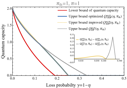
(a)

(b)

Figure 1: Bounds of quantum capacity of Gaussian loss channel $\mathcal{N}[\eta,\bar{n}_{\tiny\textrm{th}}]$ for $(\bar{n}_{\scriptsize\textrm{th}},\bar{n})=(1,1)$ (left) and $(\bar{n}_{\scriptsize\textrm{th}},\bar{n})=(1,10)$ (right). Lower bound (red) is obtained by evaluating the coherent information with a thermal input state (see Eq.(26)). The improved data-processing bound $Q^{n\leq\bar{n}}_{\tiny{\textrm{IDP}}}(\eta,\bar{n}_{\tiny\textrm{th}})$ (dashed yellow) is identical to the optimized data-processing bound $Q^{n\leq\bar{n}}_{\tiny{\textrm{ODP}}}(\eta,\bar{n}_{\tiny\textrm{th}})$ (blue) in a wide range of parameter space, and is very close to the optimal one even when it is not optimal. The data-processing bound $Q^{n\leq\bar{n}}_{\tiny{\textrm{DP}}}(\eta,\bar{n}_{\tiny\textrm{th}})$ (dashed grey) is optimal when $\eta\geq\eta^{\star}(\bar{n}_{\scriptsize\textrm{th}},\bar{n})$ for some $\eta^{\star}(\bar{n}_{\scriptsize\textrm{th}},\bar{n})$ (e.g., $\eta^{\star}(1,1)=0.8775\cdots$).

In the energy-constrained case, more care is needed when combining Lemma 8 with the data-processing argument, because the quantum-limited amplification in $\mathcal{E}^{\prime}=\mathcal{A}[\tilde{G}^{\prime}]\cdot\mathcal{E}$ increases the energy of the encoded state:

$$\bar{n}^{\prime}=\textrm{Tr}[\mathcal{A}[\tilde{G}^{\prime}](\hat{\rho})\hat{n}]=\tilde{G}^{\prime}\bar{n}+(\tilde{G}^{\prime}-1),$$ (35)

as can be derived from the symplectic transformation of the two-mode squeezing (Eq.(80) and the text above in Appendix A).

Theorem 11 (Improved data-processing bound with energy constraint).

Energy-constrained quantum capacity of Gaussian loss channel $\mathcal{N}[\eta,\bar{n}_{\scriptsize\textrm{th}}]$ is upper bounded by

$$Q^{n\leq\bar{n}}_{\scriptsize\textrm{reg}}(\mathcal{N}[\eta,\bar{n}_{\scriptsize\textrm{th}}]) \leq Q^{n\leq\bar{n}}_{\scriptsize{\textrm{IDP}}}(\eta,\bar{n}_{\scriptsize\textrm{th}})$$

$$\equiv Q^{n\leq\tilde{G}^{\prime}\bar{n}+(\tilde{G}^{\prime}-1)}(\mathcal{N}[\tilde{\eta}^{\prime},0]),$$ (36)

where $\bar{n}$ is the maximum allowed average photon number per bosonic mode in the encoded state. $Q^{n\leq\bar{n}}_{\scriptsize{\textrm{IDP}}}(\eta,\bar{n}_{\scriptsize\textrm{th}})$ simplifies to

$$Q^{n\leq\bar{n}}_{\scriptsize{\textrm{IDP}}}(\eta,\bar{n}_{\scriptsize\textrm{th}}) =\max\Big{[}g(\eta\bar{n}+(1-\eta)\bar{n}_{\scriptsize\textrm{th}})$$

$$-g\Big{(}\frac{(1-\eta)(\bar{n}_{\tiny\textrm{th}}+1)(\eta\bar{n}+(1-\eta)\bar{n}_{\tiny\textrm{th}})}{\eta-(1-\eta)\bar{n}_{\tiny\textrm{th}}}\Big{)},0\Big{]}.$$ (37)

Proof.

Let $\{\mathcal{E}^{n\leq\bar{n}},\mathcal{D}\}$ be the set of encoding and decoding which achieves the rate $R=Q^{n\leq\bar{n}}_{\scriptsize\textrm{reg}}(\mathcal{N}[\eta,\bar{n}_{\scriptsize\textrm{th}}])$ for the Gaussian loss channel $\mathcal{N}[\eta,\bar{n}_{\scriptsize\textrm{th}}]$. Then, the encoding and decoding set $\{\mathcal{A}[\tilde{G}^{\prime}]\cdot\mathcal{E}^{n\leq\bar{n}},\mathcal{D}\}$ achieves the rate $R=Q^{n\leq\bar{n}}_{\scriptsize\textrm{reg}}(\mathcal{N}[\eta,\bar{n}_{\scriptsize\textrm{th}}])$ for the bosonic pure-loss channel $\mathcal{N}[\tilde{\eta}^{\prime},0]$. Since the new encoding $\mathcal{E}^{\prime}\equiv\mathcal{A}[\tilde{G}^{\prime}]\cdot\mathcal{E}^{n\leq\bar{n}}$ has photon number $n\leq\tilde{G}^{\prime}\bar{n}+(\tilde{G}^{\prime}-1)$, the rate $R$ should be less than $Q^{n\leq\tilde{G}^{\prime}\bar{n}+(\tilde{G^{\prime}}-1)}(\mathcal{N}[\tilde{\eta}^{\prime},0])$. ∎

We note that Theorem 11 was independently discovered in Sharma et al. (2017) (see Theorem 45 therein). We emphasize that, unlike the energy-unconstrained case, our new upper bound $Q^{n\leq\bar{n}}_{\scriptsize{\textrm{IDP}}}(\eta,\bar{n}_{\scriptsize\textrm{th}})$ is not always tighter than $Q^{n\leq\bar{n}}_{\scriptsize{\textrm{DP}}}(\eta,\bar{n}_{\scriptsize\textrm{th}})$ (see the inset of Fig. 1). Physically, this is because the increased encoding energy due to pre-amplification allows larger quantum capacity, which is crucial if the allowed average photon number in the encoding is small, i.e., $\bar{n}\ll 1$. To overcome this issue, we consider a more general decomposition of the Gaussian loss channel, including both pre-amplification and post-amplification:

$$\mathcal{N}[\eta,\bar{n}_{\scriptsize\textrm{th}}]=\mathcal{A}[G_{1}]\mathcal{N}[\bar{\eta},0]\mathcal{A}[G_{2}],$$ (38)

where $\bar{\eta}=1-\frac{(1-\eta)}{G_{1}}(\bar{n}_{\scriptsize\textrm{th}}+1)$, $G_{2}=\eta/(G_{1}-(1-\eta)(\bar{n}_{\scriptsize\textrm{th}}+1))$ and $G_{1}$ can take any value in the range $1\leq G_{1}\leq 1+(1-\eta)\bar{n}_{\scriptsize\textrm{th}}$ (the upper bound of $G_{1}$ is imposed by $G_{2}\geq 1$). In this more general setting, the upper bound of the quantum capacity of $\mathcal{N}[\eta,\bar{n}_{\scriptsize\textrm{th}}]$ is given by $Q^{n\leq G_{2}\bar{n}+(G_{2}-1)}(\mathcal{N}[\bar{\eta},0])$. This upper bound can then be optimized by choosing $G_{1},G_{2}\geq 1$ such that the upper bound is minimized, i.e.,

$$Q^{n\leq\bar{n}}_{\scriptsize\textrm{reg}}(\mathcal{N}[\eta,\bar{n}_{\scriptsize\textrm{th}}])\leq\min_{G_{1},G_{2}\geq 1}Q^{n\leq G_{2}\bar{n}+(G_{2}-1)}(\mathcal{N}[\bar{\eta},0]).$$ (39)

Theorem 12 (Optimized data-processing bound with energy-constraint).

Energy-constrained quantum capacity of Gaussian loss channel $\mathcal{N}[\eta,\bar{n}_{\scriptsize\textrm{th}}]$ is upper bounded by the optimized data-processing bound $Q^{n\leq\bar{n}}_{\scriptsize{\textrm{ODP}}}(\eta,\bar{n}_{\scriptsize\textrm{th}})$:

$$Q^{n\leq\bar{n}}_{\scriptsize\textrm{reg}}(\mathcal{N}[\eta,\bar{n}_{\scriptsize\textrm{th}}]) \leq Q^{n\leq\bar{n}}_{\scriptsize{\textrm{ODP}}}(\eta,\bar{n}_{\scriptsize\textrm{th}})$$

$$\equiv\min_{1\leq G_{1}\leq 1+(1-\eta)\bar{n}_{\scriptsize\textrm{th}}}f_{\eta,\bar{n}_{\scriptsize\textrm{th}},\bar{n}}(G_{1}),$$ (40)

where $\bar{n}$ is the maximum allowed average photon number in the encoding and $f_{\eta,\bar{n}_{\scriptsize\textrm{th}},\bar{n}}(G_{1})$ is defined as

$$f_{\eta,\bar{n}_{\scriptsize\textrm{th}},\bar{n}}(G_{1}) \equiv\max\Big{[}g\big{(}\bar{\eta}(G_{2}\bar{n}+(G_{2}-1))\big{)}$$

$$\qquad-g\big{(}(1-\bar{\eta})(G_{2}\bar{n}+(G_{2}-1))\big{)},0\Big{]}.$$ (41)

and $\bar{\eta}=1-\frac{(1-\eta)}{G_{1}}(\bar{n}_{\scriptsize\textrm{th}}+1)$, $G_{2}=\eta/(G_{1}-(1-\eta)(\bar{n}_{\scriptsize\textrm{th}}+1))$.

Proof.

See appendix C for the derivation. ∎

Since $Q^{n\leq\bar{n}}_{\scriptsize{\textrm{DP}}}(\eta,\bar{n}_{\scriptsize\textrm{th}})$ and $Q^{n\leq\bar{n}}_{\scriptsize{\textrm{IDP}}}(\eta,\bar{n}_{\scriptsize\textrm{th}})$ are the two extremes with $G_{2}=1$ and $G_{1}=1$, respectively, they are greater than or equal to the optimized data-processing bound. Thus $Q^{n\leq\bar{n}}_{\scriptsize{\textrm{ODP}}}(\eta,\bar{n}_{\scriptsize\textrm{th}})$ is the best upper bound among all the data-processing type bounds introduced above (see Fig. 1). We numerically observe, however, that either one of these two extremes is optimal: $Q^{n\leq\bar{n}}_{\scriptsize{\textrm{ODP}}}(\eta,\bar{n}_{\scriptsize\textrm{th}})=Q^{n\leq\bar{n}}_{\scriptsize{\textrm{DP}}}(\eta,\bar{n}_{\scriptsize\textrm{th}})$ for $\eta\geq\eta^{\star}(\bar{n}_{\scriptsize\textrm{th}},n)$ and $Q^{n\leq\bar{n}}_{\scriptsize{\textrm{ODP}}}(\eta,\bar{n}_{\scriptsize\textrm{th}})=Q^{n\leq\bar{n}}_{\scriptsize{\textrm{IDP}}}(\eta,\bar{n}_{\scriptsize\textrm{th}})$ otherwise for some $\eta^{\star}(\bar{n}_{\scriptsize\textrm{th}},n)$. In $\bar{n}\rightarrow\infty$ limit, $\lim_{\bar{n}\rightarrow\infty}\eta^{\star}(\bar{n}_{\scriptsize\textrm{th}},\bar{n})=1$ and thus $Q^{n\leq\bar{n}}_{\scriptsize{\textrm{ODP}}}(\eta,\bar{n}_{\scriptsize\textrm{th}})=Q^{n\leq\bar{n}}_{\scriptsize{\textrm{IDP}}}(\eta,\bar{n}_{\scriptsize\textrm{th}})$ for all $\eta\in[0,1]$, consistent with Eq.(33). We refer to Ref. Sharma et al. (2017) (e.g., Fig. 6 therein) for a more comprehensive comparison of existing upper bounds, including approximate degradability bounds Sutter et al. (2017).

Finally, the following upper bound of energy-unconstrained quantum capacity of the Gaussian random displacement channel can be derived from the data-processing argument combined with Lemma 6 (specialized to $\bar{n}_{\scriptsize\textrm{th}}=0$):

$$Q_{\scriptsize\textrm{reg}}(\mathcal{N}_{B_{2}}[\sigma^{2}])\leq\max\Big{[}\log\Big{(}\frac{1-\sigma^{2}}{\sigma^{2}}\Big{)},0\Big{]}.$$ (42)

Note that this bound is strictly tighter than the one in Eq.(30).

IV Gottesman-Kitaev-Preskill codes

We now aim to find an explicit encoding and decoding strategy which achieves the quantum capacity of Gaussian loss channels. It is very important to realize that the coherent information of bosonic pure-loss channel being maximized by a Gaussian state (i.e., thermal state; Theorem 9) does not imply that Gaussian encoding and decoding is sufficient to achieve the quantum capacity of bosonic pure-loss channel. In fact, it was proven that entanglement distillation of Gaussian states with Gaussian operation is impossible Eisert et al. (2002). Due to the close relation between entanglement distillation and quantum state transmission via the quantum teleportation protocol, this implies that Gaussian encoding and decoding can never achieve a non-vanishing quantum communication rate for Gaussian channels. In other words, quantum error correction of a Gaussian error is impossible if the states and operations are restricted to be Gaussian Niset et al. (2009). Therefore, non-Gaussian resources are necessary in order to achieve reliable quantum information transmission through noisy Gaussian channels.

In this section, we show that the ability to prepare a Gottesman-Kitaev-Preskill (GKP) state, which is a non-Gaussian state, is sufficient to establish non-vanishing quantum communication rate through Gaussian loss channels. In particular, we prove that the GKP codes achieve the quantum capacity of Gaussian loss channels up to at most a constant gap from the upper bound given in Theorem 32, in the energy-unconstrained scenario.

IV.1 One-mode square lattice GKP code

The one-mode square lattice GKP code is the simplest class of the GKP codes Gottesman et al. (2001). The code space $\mathcal{C}_{\scriptsize\textrm{sq}}^{[d]}\subset\mathcal{H}$ is defined as $\mathcal{C}_{\scriptsize\textrm{sq}}^{[d]}=\{|\psi\rangle\,|\,\hat{S}^{[d]}_{\scriptsize\textrm{sq},q}|\psi\rangle=|\psi\rangle,\hat{S}^{[d]}_{\scriptsize\textrm{sq},p}|\psi\rangle=|\psi\rangle\}$, where

$$\hat{S}^{[d]}_{\scriptsize\textrm{sq},q} \equiv\exp(i\hat{q}\mathchoice{{\hbox{$\displaystyle\sqrt{2\pi d\,}$}\lower 0.4pt\hbox{\vrule height=6.94444pt,depth=-5.55559pt}}}{{\hbox{$\textstyle\sqrt{2\pi d\,}$}\lower 0.4pt\hbox{\vrule height=6.94444pt,depth=-5.55559pt}}}{{\hbox{$\scriptstyle\sqrt{2\pi d\,}$}\lower 0.4pt\hbox{\vrule height=4.8611pt,depth=-3.8889pt}}}{{\hbox{$\scriptscriptstyle\sqrt{2\pi d\,}$}\lower 0.4pt\hbox{\vrule height=3.47221pt,depth=-2.77779pt}}})=\hat{D}(i\mathchoice{{\hbox{$\displaystyle\sqrt{\pi d\,}$}\lower 0.4pt\hbox{\vrule height=6.94444pt,depth=-5.55559pt}}}{{\hbox{$\textstyle\sqrt{\pi d\,}$}\lower 0.4pt\hbox{\vrule height=6.94444pt,depth=-5.55559pt}}}{{\hbox{$\scriptstyle\sqrt{\pi d\,}$}\lower 0.4pt\hbox{\vrule height=4.8611pt,depth=-3.8889pt}}}{{\hbox{$\scriptscriptstyle\sqrt{\pi d\,}$}\lower 0.4pt\hbox{\vrule height=3.47221pt,depth=-2.77779pt}}}),$$

$$\hat{S}^{[d]}_{\scriptsize\textrm{sq},p} \equiv\exp(-i\hat{p}\mathchoice{{\hbox{$\displaystyle\sqrt{2\pi d\,}$}\lower 0.4pt\hbox{\vrule height=6.94444pt,depth=-5.55559pt}}}{{\hbox{$\textstyle\sqrt{2\pi d\,}$}\lower 0.4pt\hbox{\vrule height=6.94444pt,depth=-5.55559pt}}}{{\hbox{$\scriptstyle\sqrt{2\pi d\,}$}\lower 0.4pt\hbox{\vrule height=4.8611pt,depth=-3.8889pt}}}{{\hbox{$\scriptscriptstyle\sqrt{2\pi d\,}$}\lower 0.4pt\hbox{\vrule height=3.47221pt,depth=-2.77779pt}}})=\hat{D}(\mathchoice{{\hbox{$\displaystyle\sqrt{\pi d\,}$}\lower 0.4pt\hbox{\vrule height=6.94444pt,depth=-5.55559pt}}}{{\hbox{$\textstyle\sqrt{\pi d\,}$}\lower 0.4pt\hbox{\vrule height=6.94444pt,depth=-5.55559pt}}}{{\hbox{$\scriptstyle\sqrt{\pi d\,}$}\lower 0.4pt\hbox{\vrule height=4.8611pt,depth=-3.8889pt}}}{{\hbox{$\scriptscriptstyle\sqrt{\pi d\,}$}\lower 0.4pt\hbox{\vrule height=3.47221pt,depth=-2.77779pt}}}),$$ (43)

are the stabilizers and $d$ is the dimension of the code space, i.e., $\textrm{dim}(\mathcal{C}_{\scriptsize\textrm{sq}}^{[d]})=d$. Although simultaneous measurement of position and momentum is impossible (i.e., $[\hat{q},\hat{p}]=i\neq 0$), they can nevertheless be measured simultaneously in modulo $\textstyle\sqrt{2\pi/d\,}$  through the stabilizer measurement, since the two stabilizers commute with each other $\hat{S}^{[d]}_{\scriptsize\textrm{sq},q}\hat{S}^{[d]}_{\scriptsize\textrm{sq},p}=\hat{S}^{[d]}_{\scriptsize\textrm{sq},p}\hat{S}^{[d]}_{\scriptsize\textrm{sq},q}e^{i2\pi d}=\hat{S}^{[d]}_{\scriptsize\textrm{sq},p}\hat{S}^{[d]}_{\scriptsize\textrm{sq},q}$. Thus, one-mode square lattice GKP codes can correct any displacement errors in the square unit cell $|\Delta q|,|\Delta p|<\mathchoice{{\hbox{$\displaystyle\sqrt{\pi/(2d)\,}$}\lower 0.4pt\hbox{\vrule height=7.5pt,depth=-6.00003pt}}}{{\hbox{$\textstyle\sqrt{\pi/(2d)\,}$}\lower 0.4pt\hbox{\vrule height=7.5pt,depth=-6.00003pt}}}{{\hbox{$\scriptstyle\sqrt{\pi/(2d)\,}$}\lower 0.4pt\hbox{\vrule height=5.25pt,depth=-4.20003pt}}}{{\hbox{$\scriptscriptstyle\sqrt{\pi/(2d)\,}$}\lower 0.4pt\hbox{\vrule height=3.75pt,depth=-3.00002pt}}}$.

Square lattice GKP code states are explicitly given by

$$|\mu^{\scriptsize\textrm{sq}}_{L}\rangle\propto\sum_{n=-\infty}^{\infty}|\hat{q}=(dn+\mu)\mathchoice{{\hbox{$\displaystyle\sqrt{2\pi/d\,}$}\lower 0.4pt\hbox{\vrule height=7.5pt,depth=-6.00003pt}}}{{\hbox{$\textstyle\sqrt{2\pi/d\,}$}\lower 0.4pt\hbox{\vrule height=7.5pt,depth=-6.00003pt}}}{{\hbox{$\scriptstyle\sqrt{2\pi/d\,}$}\lower 0.4pt\hbox{\vrule height=5.25pt,depth=-4.20003pt}}}{{\hbox{$\scriptscriptstyle\sqrt{2\pi/d\,}$}\lower 0.4pt\hbox{\vrule height=3.75pt,depth=-3.00002pt}}}\rangle$$ (44)

in the computational basis, where $\mu=0,\cdots,d-1$ and $|\hat{q}=q_{0}\rangle$ is an eigenstate of the position operator $\hat{q}$ localized at $q=q_{0}$, which is an infinitely squeezed state. Phase rotation by angle $\theta=-\pi/2$ implements the basis transformation from $|\mu^{\scriptsize\textrm{sq}}_{L}\rangle$ to

$$|\bar{\mu}^{\scriptsize\textrm{sq}}_{L}\rangle\propto\sum_{n=-\infty}^{\infty}|\hat{p}=(dn-\mu)\mathchoice{{\hbox{$\displaystyle\sqrt{2\pi/d\,}$}\lower 0.4pt\hbox{\vrule height=7.5pt,depth=-6.00003pt}}}{{\hbox{$\textstyle\sqrt{2\pi/d\,}$}\lower 0.4pt\hbox{\vrule height=7.5pt,depth=-6.00003pt}}}{{\hbox{$\scriptstyle\sqrt{2\pi/d\,}$}\lower 0.4pt\hbox{\vrule height=5.25pt,depth=-4.20003pt}}}{{\hbox{$\scriptscriptstyle\sqrt{2\pi/d\,}$}\lower 0.4pt\hbox{\vrule height=3.75pt,depth=-3.00002pt}}}\rangle,$$ (45)

where $|\hat{p}=p_{0}\rangle$ is the eigenstate of the momentum $\hat{p}$ at $p=p_{0}$. Note that $|\bar{\mu}^{\scriptsize\textrm{sq}}_{L}\rangle=\mathchoice{{\hbox{$\displaystyle\sqrt{1/d\,}$}\lower 0.4pt\hbox{\vrule height=7.5pt,depth=-6.00003pt}}}{{\hbox{$\textstyle\sqrt{1/d\,}$}\lower 0.4pt\hbox{\vrule height=7.5pt,depth=-6.00003pt}}}{{\hbox{$\scriptstyle\sqrt{1/d\,}$}\lower 0.4pt\hbox{\vrule height=5.25pt,depth=-4.20003pt}}}{{\hbox{$\scriptscriptstyle\sqrt{1/d\,}$}\lower 0.4pt\hbox{\vrule height=3.75pt,depth=-3.00002pt}}}\sum_{\nu=0}^{d-1}\exp(-i2\pi\mu\nu/d)|\nu^{\scriptsize\textrm{sq}}_{L}\rangle$.

Since GKP code states are superpositions of infinitely many infinitely squeezed states, their average photon number diverge. It is possible, however, to construct a finite energy GKP states: Replace infinitely squeezed states by finitely squeezed ones, and introduce an overall Gaussian envelop (see Eq.(31) in Gottesman et al. (2001)). Our brief new observation is that this can be concisely realized by $|\mu_{L}^{\Delta}\rangle\propto\exp(-\Delta^{2}\hat{n})|\mu_{L}\rangle$ (which is an equivalent form of Eqs.(40),(41) in Gottesman et al. (2001)). The non-unitary operation $\exp(-\Delta^{2}\hat{n})$ can be physically implemented by passing the input state through a beam splitter with vacuum ancilla, and then by counting photon number and post-selecting the vacuum click at the out-going idler port. As a result, large enough GKP states of any shape can be carved into smaller ones with Gaussian envelop, where the size of the resulting GKP states (i.e., $\Delta$) can be modulated by transmissivity of the beam splitter.

In Fig. 2, we plot the Wigner function of maximally mixed code state $\hat{\rho}_{\mathcal{C}}=\hat{P}_{\mathcal{C}}/d$ of the square lattice and hexagonal lattice (see subsection IV.2) GKP code states for $d=2$ and $\bar{n}=3$, where $\hat{P}_{\mathcal{C}}$ is the projection operator to the code space $\mathcal{C}$. In the remainder of this section, we restrict ourselves to the properties of energy-unconstrained ideal GKP states.

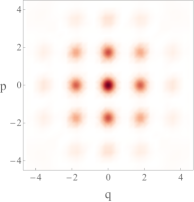
(a)

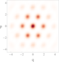
(b)

(c)

Figure 2: Wigner function of maximally mixed code states of the one-mode square lattice (left; $\mathcal{C}_{\tiny\textrm{sq}}^{[d]}$) and hexagonal lattice (right; $\mathcal{C}_{\tiny\textrm{hex}}^{[d]}$) GKP code with $d=2$ and average photon number $\bar{n}=3$.

Universal gate set of the square lattice GKP code is given as follows: Logical Pauli gates (i.e., Clifford gates of hierarchy 1) are given by $\hat{Z}^{\scriptsize\textrm{sq}}_{L}=(\hat{S}^{[d]}_{\scriptsize\textrm{sq},q})^{\frac{1}{d}}=\exp(i\hat{q}\mathchoice{{\hbox{$\displaystyle\sqrt{2\pi/d\,}$}\lower 0.4pt\hbox{\vrule height=7.5pt,depth=-6.00003pt}}}{{\hbox{$\textstyle\sqrt{2\pi/d\,}$}\lower 0.4pt\hbox{\vrule height=7.5pt,depth=-6.00003pt}}}{{\hbox{$\scriptstyle\sqrt{2\pi/d\,}$}\lower 0.4pt\hbox{\vrule height=5.25pt,depth=-4.20003pt}}}{{\hbox{$\scriptscriptstyle\sqrt{2\pi/d\,}$}\lower 0.4pt\hbox{\vrule height=3.75pt,depth=-3.00002pt}}})$ and $\hat{X}^{\scriptsize\textrm{sq}}_{L}=(\hat{S}^{[d]}_{\scriptsize\textrm{sq},p})^{\frac{1}{d}}=\exp(-i\hat{p}\mathchoice{{\hbox{$\displaystyle\sqrt{2\pi/d\,}$}\lower 0.4pt\hbox{\vrule height=7.5pt,depth=-6.00003pt}}}{{\hbox{$\textstyle\sqrt{2\pi/d\,}$}\lower 0.4pt\hbox{\vrule height=7.5pt,depth=-6.00003pt}}}{{\hbox{$\scriptstyle\sqrt{2\pi/d\,}$}\lower 0.4pt\hbox{\vrule height=5.25pt,depth=-4.20003pt}}}{{\hbox{$\scriptscriptstyle\sqrt{2\pi/d\,}$}\lower 0.4pt\hbox{\vrule height=3.75pt,depth=-3.00002pt}}})$, i.e., displacement operators, yielding $\hat{Z}^{\scriptsize\textrm{sq}}_{L}|\mu^{\scriptsize\textrm{sq}}_{L}\rangle=\exp(i2\pi\mu/d)|\mu^{\scriptsize\textrm{sq}}_{L}\rangle$, $\hat{X}^{\scriptsize\textrm{sq}}_{L}|\mu^{\scriptsize\textrm{sq}}_{L}\rangle=|(\mu\oplus 1)^{\scriptsize\textrm{sq}}_{L}\rangle$, where $\oplus$ is the summation in modulo $d$. (The notion of Clifford hierarchy is due to Gottesman and Chuang (1999).) Any logical Clifford gates of hierarchy 2 can be implemented by Gaussian unitary operations Gottesman et al. (2001). For example, logical Hadamard gate can be implemented by phase rotation $\exp(-i\pi\hat{a}^{\dagger}\hat{a}/2)$, as explained above. Logical CNOT gate can be realized by the SUM gate: $\exp(-i\hat{p}_{1}\hat{q}_{2})|\mu^{\scriptsize\textrm{sq}}_{L}\rangle|\nu^{\scriptsize\textrm{sq}}_{L}\rangle=|(\mu\oplus\nu)^{\scriptsize\textrm{sq}}_{L}\rangle|\nu^{\scriptsize\textrm{sq}}_{L}\rangle$. In $d=2$ case, we observe that $\exp(i\hat{q}^{4}/(4\pi))$ is the logical T gate (a Clifford gate of hierarchy 3), i.e., $\exp(i\hat{q}^{4}/(4\pi))|\mu^{\scriptsize\textrm{sq}}_{L}\rangle=\exp(i\pi\mu/4)|\mu^{\scriptsize\textrm{sq}}_{L}\rangle$, completing the gate set for universal quantum computation.

Encoding of arbitrary logical states can be achieved as follows: Let $|\psi\rangle=\sum_{\mu=0}^{d-1}c_{\mu}|\mu\rangle$ be an arbitrary state of a physical qudit and assume that one of the GKP logical states (e.g., $|0^{\scriptsize\textrm{sq}}_{L}\rangle$) is available. Also, assume the gate $\sum_{\nu=0}^{d-1}(\hat{X}^{\scriptsize\textrm{sq}}_{L})^{\nu}\otimes|\nu\rangle\langle\nu|$, generated by a Hamiltonian of the form $\hat{H}\propto i(\hat{a}_{1}-\hat{a}_{1}^{\dagger})\otimes\hat{a}_{2}^{\dagger}\hat{a}_{2}$, can be implemented, where $\hat{a}_{1}$ is a bosonic annihilation operator associated with the encoded mode and $\hat{a}_{2}\equiv\sum_{\mu=0}^{d-1}\mathchoice{{\hbox{$\displaystyle\sqrt{\mu\,}$}\lower 0.4pt\hbox{\vrule height=4.30554pt,depth=-3.44446pt}}}{{\hbox{$\textstyle\sqrt{\mu\,}$}\lower 0.4pt\hbox{\vrule height=4.30554pt,depth=-3.44446pt}}}{{\hbox{$\scriptstyle\sqrt{\mu\,}$}\lower 0.4pt\hbox{\vrule height=3.01389pt,depth=-2.41113pt}}}{{\hbox{$\scriptscriptstyle\sqrt{\mu\,}$}\lower 0.4pt\hbox{\vrule height=2.15277pt,depth=-1.72223pt}}}|\mu-1\rangle\langle\mu|$, associated with the physical qudit. Then, we get

$$\Big{[}\sum_{\nu=0}^{d-1}(\hat{X}^{\scriptsize\textrm{sq}}_{L})^{\nu}\otimes|\nu\rangle\langle\nu|\Big{]}(|0^{\scriptsize\textrm{sq}}_{L}\rangle\otimes|\psi\rangle)=\sum_{\mu=0}^{d-1}c_{\mu}|\mu^{\scriptsize\textrm{sq}}_{L}\rangle\otimes|\mu\rangle.$$ (46)

Upon a unitary Fourier gate on the physical qudit, $|\mu\rangle\rightarrow\mathchoice{{\hbox{$\displaystyle\sqrt{1/d\,}$}\lower 0.4pt\hbox{\vrule height=7.5pt,depth=-6.00003pt}}}{{\hbox{$\textstyle\sqrt{1/d\,}$}\lower 0.4pt\hbox{\vrule height=7.5pt,depth=-6.00003pt}}}{{\hbox{$\scriptstyle\sqrt{1/d\,}$}\lower 0.4pt\hbox{\vrule height=5.25pt,depth=-4.20003pt}}}{{\hbox{$\scriptscriptstyle\sqrt{1/d\,}$}\lower 0.4pt\hbox{\vrule height=3.75pt,depth=-3.00002pt}}}\sum_{\nu=0}^{d-1}\exp(-i2\pi\mu\nu/d)|\nu\rangle$, this state becomes $\sum_{\mu,\nu=0}^{d-1}c_{\mu}\exp(-i2\pi\mu\nu/d)|\mu^{\scriptsize\textrm{sq}}_{L}\rangle\otimes|\nu\rangle$. If one then measures the physical qudit in computational basis $\{|0\rangle,\cdots,|d-1\rangle\}$ and the measurement outcome is $|\nu\rangle$, the oscillator state is collapsed into $|\psi^{\scriptsize\textrm{sq}}_{L}(\nu)\rangle=\sum_{\mu=0}^{d-1}c_{\mu}\exp(-i2\pi\mu\nu/d)|\mu^{\scriptsize\textrm{sq}}_{L}\rangle$. Applying $(\hat{Z}^{\scriptsize\textrm{sq}}_{L})^{\nu}$, we finally obtain the desired encoded logical state

$$(\hat{Z}^{\scriptsize\textrm{sq}}_{L})^{\nu}|\psi^{\scriptsize\textrm{sq}}_{L}(\nu)\rangle=\sum_{\mu=0}^{d-1}c_{\mu}|\mu^{\scriptsize\textrm{sq}}_{L}\rangle.$$ (47)

If the encoded GKP states are sent though the Gaussian random displacement channel, decoding can be achieved by measuring two stabilizers $\hat{S}_{\scriptsize\textrm{sq},q}^{[d]},\hat{S}_{\scriptsize\textrm{sq},p}^{[d]}$ given in Eq.(43), providing protection against the channel noise as specified in the text below Eq.(43). Given that fresh supply of ancillary GKP state is available, such stabilizer measurements can be achieved by Gaussian operations and homodyne detection: Assume we have an ancillary oscillator mode prepared at $|\bar{0}^{\scriptsize\textrm{sq}}_{L}\rangle$ (i.e., $q_{2}\equiv 0\,\,\textrm{mod}\mathchoice{{\hbox{$\displaystyle\sqrt{2\pi/d\,}$}\lower 0.4pt\hbox{\vrule height=7.5pt,depth=-6.00003pt}}}{{\hbox{$\textstyle\sqrt{2\pi/d\,}$}\lower 0.4pt\hbox{\vrule height=7.5pt,depth=-6.00003pt}}}{{\hbox{$\scriptstyle\sqrt{2\pi/d\,}$}\lower 0.4pt\hbox{\vrule height=5.25pt,depth=-4.20003pt}}}{{\hbox{$\scriptscriptstyle\sqrt{2\pi/d\,}$}\lower 0.4pt\hbox{\vrule height=3.75pt,depth=-3.00002pt}}}$). Upon the SUM gate $\exp(-i\hat{q}_{1}\hat{p}_{2})$, the ancillary position operator $\hat{q}_{2}$ is transformed into $\hat{q}_{2}+\hat{q}_{1}$ while the system’s position operator remains at $\hat{q}_{1}$. We can then perform homodyne measurement of $\hat{q}_{2}$, and if the measurement outcome is $q_{2}^{M}(=q_{1}+q_{2})$, we can extract the value of $\hat{q}_{1}$ in modulo $\textstyle\sqrt{2\pi/d\,}$ , i.e., $q_{1}\equiv q_{2}^{M}\,\,\textrm{mod}\mathchoice{{\hbox{$\displaystyle\sqrt{2\pi/d\,}$}\lower 0.4pt\hbox{\vrule height=7.5pt,depth=-6.00003pt}}}{{\hbox{$\textstyle\sqrt{2\pi/d\,}$}\lower 0.4pt\hbox{\vrule height=7.5pt,depth=-6.00003pt}}}{{\hbox{$\scriptstyle\sqrt{2\pi/d\,}$}\lower 0.4pt\hbox{\vrule height=5.25pt,depth=-4.20003pt}}}{{\hbox{$\scriptscriptstyle\sqrt{2\pi/d\,}$}\lower 0.4pt\hbox{\vrule height=3.75pt,depth=-3.00002pt}}}$, hence measuring $\hat{S}_{\scriptsize\textrm{sq},q}^{[d]}$. The other stabilizer $\hat{S}_{\scriptsize\textrm{sq},p}^{[d]}$ can also be measured in a similar way using an initial ancillary GKP state $|0^{\scriptsize\textrm{sq}}_{L}\rangle$ (i.e., $p_{2}\equiv 0\,\,\textrm{mod}\mathchoice{{\hbox{$\displaystyle\sqrt{2\pi/d\,}$}\lower 0.4pt\hbox{\vrule height=7.5pt,depth=-6.00003pt}}}{{\hbox{$\textstyle\sqrt{2\pi/d\,}$}\lower 0.4pt\hbox{\vrule height=7.5pt,depth=-6.00003pt}}}{{\hbox{$\scriptstyle\sqrt{2\pi/d\,}$}\lower 0.4pt\hbox{\vrule height=5.25pt,depth=-4.20003pt}}}{{\hbox{$\scriptscriptstyle\sqrt{2\pi/d\,}$}\lower 0.4pt\hbox{\vrule height=3.75pt,depth=-3.00002pt}}}$), SUM gate with control and target exchanged $\exp(-i\hat{p}_{1}\hat{q}_{2})$ and homodyne measurement of $\hat{p}_{2}$ (see the text below Eq.(105) in Gottesman et al. (2001)). From the extracted values of position and momentum in modulo $\textstyle\sqrt{2\pi/d\,}$  (i.e., $q_{2}^{M},p_{2}^{M}$), one can infer $\Delta q=q_{2}^{M\star}$, $\Delta p=p_{2}^{M\star}$, where $q_{2}^{M\star},p_{2}^{M\star}$ are defined such that $q_{2}^{M}\equiv q_{2}^{M\star}\,\,\textrm{mod}\mathchoice{{\hbox{$\displaystyle\sqrt{2\pi/d\,}$}\lower 0.4pt\hbox{\vrule height=7.5pt,depth=-6.00003pt}}}{{\hbox{$\textstyle\sqrt{2\pi/d\,}$}\lower 0.4pt\hbox{\vrule height=7.5pt,depth=-6.00003pt}}}{{\hbox{$\scriptstyle\sqrt{2\pi/d\,}$}\lower 0.4pt\hbox{\vrule height=5.25pt,depth=-4.20003pt}}}{{\hbox{$\scriptscriptstyle\sqrt{2\pi/d\,}$}\lower 0.4pt\hbox{\vrule height=3.75pt,depth=-3.00002pt}}}$, $p_{2}^{M}\equiv p_{2}^{M\star}\,\,\textrm{mod}\mathchoice{{\hbox{$\displaystyle\sqrt{2\pi/d\,}$}\lower 0.4pt\hbox{\vrule height=7.5pt,depth=-6.00003pt}}}{{\hbox{$\textstyle\sqrt{2\pi/d\,}$}\lower 0.4pt\hbox{\vrule height=7.5pt,depth=-6.00003pt}}}{{\hbox{$\scriptstyle\sqrt{2\pi/d\,}$}\lower 0.4pt\hbox{\vrule height=5.25pt,depth=-4.20003pt}}}{{\hbox{$\scriptscriptstyle\sqrt{2\pi/d\,}$}\lower 0.4pt\hbox{\vrule height=3.75pt,depth=-3.00002pt}}}$ and $|q_{2}^{M\star}|,|p_{2}^{M\star}|\leq\mathchoice{{\hbox{$\displaystyle\sqrt{\pi/(2d)\,}$}\lower 0.4pt\hbox{\vrule height=7.5pt,depth=-6.00003pt}}}{{\hbox{$\textstyle\sqrt{\pi/(2d)\,}$}\lower 0.4pt\hbox{\vrule height=7.5pt,depth=-6.00003pt}}}{{\hbox{$\scriptstyle\sqrt{\pi/(2d)\,}$}\lower 0.4pt\hbox{\vrule height=5.25pt,depth=-4.20003pt}}}{{\hbox{$\scriptscriptstyle\sqrt{\pi/(2d)\,}$}\lower 0.4pt\hbox{\vrule height=3.75pt,depth=-3.00002pt}}}$. One can then correct such errors by counter displacement $\exp(i\hat{p}_{1}q_{2}^{M\star})$ and $\exp(-i\hat{q}_{1}p_{2}^{M\star})$.

In both encoding and decoding, the most non-trivial task is to prepare a GKP state (e.g., $|0^{\scriptsize\textrm{sq}}_{L}\rangle$) from an arbitrary non-GKP state. There have been many proposals to achieve such a goal in various experimental platforms Travaglione and Milburn (2002); Pirandola et al. (2004, 2006); Vasconcelos et al. (2010); Terhal and Weigand (2016); Motes et al. (2017); Weigand and Terhal (2017), including the one in the original paper Gottesman et al. (2001). In particular, the proposal in Terhal and Weigand (2016) is based on the idea of phase estimation of unitary operators Kitaev (1996), which allows the following representation of the GKP states (equivalent to Eq.(29) in Gottesman et al. (2001))

$$|\mu^{\scriptsize\textrm{sq}}_{L}\rangle \propto(\hat{X}^{\scriptsize\textrm{sq}}_{L})^{\mu}\sum_{n_{1},n_{2}=-\infty}^{\infty}(\hat{S}_{\scriptsize\textrm{sq},p}^{[d]})^{n_{1}}(\hat{Z}^{\scriptsize\textrm{sq}}_{L})^{n_{2}}|\phi_{0}\rangle$$

$$=\sum_{n_{1},n_{2}=-\infty}^{\infty}e^{-i\hat{p}\mathchoice{{\hbox{$\displaystyle\sqrt{\frac{2\pi}{d}\,}$}\lower 0.4pt\hbox{\vrule height=6.94165pt,depth=-5.55334pt}}}{{\hbox{$\textstyle\sqrt{\frac{2\pi}{d}\,}$}\lower 0.4pt\hbox{\vrule height=4.85916pt,depth=-3.88734pt}}}{{\hbox{$\scriptstyle\sqrt{\frac{2\pi}{d}\,}$}\lower 0.4pt\hbox{\vrule height=3.47083pt,depth=-2.77667pt}}}{{\hbox{$\scriptscriptstyle\sqrt{\frac{2\pi}{d}\,}$}\lower 0.4pt\hbox{\vrule height=3.47083pt,depth=-2.77667pt}}}(dn_{1}+\mu)}e^{i\hat{q}\mathchoice{{\hbox{$\displaystyle\sqrt{\frac{2\pi}{d}\,}$}\lower 0.4pt\hbox{\vrule height=6.94165pt,depth=-5.55334pt}}}{{\hbox{$\textstyle\sqrt{\frac{2\pi}{d}\,}$}\lower 0.4pt\hbox{\vrule height=4.85916pt,depth=-3.88734pt}}}{{\hbox{$\scriptstyle\sqrt{\frac{2\pi}{d}\,}$}\lower 0.4pt\hbox{\vrule height=3.47083pt,depth=-2.77667pt}}}{{\hbox{$\scriptscriptstyle\sqrt{\frac{2\pi}{d}\,}$}\lower 0.4pt\hbox{\vrule height=3.47083pt,depth=-2.77667pt}}}n_{2}}|\phi_{0}\rangle.$$ (48)

Here, $\sum_{n_{1}=-\infty}^{\infty}(\hat{S}_{p}^{[d]})^{n_{1}}$ and $\sum_{n_{2}=-\infty}^{\infty}(\hat{Z}_{L})^{n_{2}}$ can be understood as the projection operator associated with the phase estimation (and correction) of $\hat{S}_{p}^{[d]}$ and $\hat{Z}_{L}$, which enforce $\hat{S}_{p}^{[d]}=\hat{Z}_{L}=1$, hence $|0^{\scriptsize\textrm{sq}}_{L}\rangle$. The last operation $(\hat{X}^{\scriptsize\textrm{sq}}_{L})^{\mu}$ then transforms $|0^{\scriptsize\textrm{sq}}_{L}\rangle$ into $|\mu^{\scriptsize\textrm{sq}}_{L}\rangle$. Note that Eq.(48) is valid for any input state $|\phi_{0}\rangle$ with non-zero overlap with $|0^{\scriptsize\textrm{sq}}_{L}\rangle$ which, for example, can be chosen to be the vacuum state. In this case, Eq.(48) can be understood as a superposition of coherent states $|\alpha\rangle$ in a $2$-dimensional square lattice $\alpha=\mathchoice{{\hbox{$\displaystyle\sqrt{\frac{\pi}{d}\,}$}\lower 0.4pt\hbox{\vrule height=7.77776pt,depth=-6.22223pt}}}{{\hbox{$\textstyle\sqrt{\frac{\pi}{d}\,}$}\lower 0.4pt\hbox{\vrule height=5.44443pt,depth=-4.35556pt}}}{{\hbox{$\scriptstyle\sqrt{\frac{\pi}{d}\,}$}\lower 0.4pt\hbox{\vrule height=3.88887pt,depth=-3.11111pt}}}{{\hbox{$\scriptscriptstyle\sqrt{\frac{\pi}{d}\,}$}\lower 0.4pt\hbox{\vrule height=3.88887pt,depth=-3.11111pt}}}(dn_{1}+\mu+in_{2})$, where $n_{1},n_{2}$ are integers.

We remark that the scheme in Travaglione and Milburn (2002) implements Eq.(48) by post-selection, whereas Terhal and Weigand (2016) does so deterministically. The former protocol is within the reach of near-term technology of trapped ion systems, and some preliminary experimental progress has been made Flühmann et al. (2017). In principle, the latter protocol can be realized in circuit quantum electrodynamics systems by, e.g., extending the quantum non-demolition measurement techniques used in Sun et al. (2014).

Based on the numerically optimized decoding operation, we earlier showed that the GKP codes offer excellent protection against bosonic pure-loss channel $\mathcal{N}[\eta,0]$ as well, despite not being specifically designed for such a purpose Albert et al. (2017). In addition, by using sub-optical decoding (i.e., quantum-limited amplification $\mathcal{A}[1/\eta]$ followed by the conventional GKP decoding as described above), we can prove that the logical error probability scales as

$$\epsilon_{L}^{\scriptsize\textrm{sq}}\sim\exp\Big{[}-\frac{\pi}{4d}\Big{(}\frac{\eta}{1-\eta}\Big{)}\Big{]},$$ (49)

(cf, Eq.(7.24) in Albert et al. (2017)) which vanishes non-analytically in the limit of perfect transmission $\eta\rightarrow 1$. In the following subsection, we will explain that it is possible to improve the constant prefactor from $\frac{\pi}{4}$ to $\frac{\pi}{2\mathchoice{{\hbox{$\displaystyle\sqrt{3\,}$}\lower 0.4pt\hbox{\vrule height=4.51111pt,depth=-3.6089pt}}}{{\hbox{$\textstyle\sqrt{3\,}$}\lower 0.4pt\hbox{\vrule height=4.51111pt,depth=-3.6089pt}}}{{\hbox{$\scriptstyle\sqrt{3\,}$}\lower 0.4pt\hbox{\vrule height=3.15778pt,depth=-2.52625pt}}}{{\hbox{$\scriptscriptstyle\sqrt{3\,}$}\lower 0.4pt\hbox{\vrule height=2.25555pt,depth=-1.80446pt}}}}$ by using hexagonal lattice GKP code instead of square lattice.

IV.2 One-mode hexagonal lattice GKP code

Code space of one-mode hexagonal lattice GKP code is defined by $\mathcal{C}_{\scriptsize{\textrm{hex}}}^{[d]}\equiv\{|\psi\rangle\,|\,\hat{S}^{[d]}_{\scriptsize\textrm{hex},q}|\psi\rangle=|\psi\rangle,\,\,\hat{S}^{[d]}_{\scriptsize\textrm{hex},p}|\psi\rangle=|\psi\rangle\}$, where the stabilizers are given by

$$\hat{S}^{[d]}_{\scriptsize\textrm{hex},q} \equiv\exp[i\mathchoice{{\hbox{$\displaystyle\sqrt{2\pi d\,}$}\lower 0.4pt\hbox{\vrule height=6.94444pt,depth=-5.55559pt}}}{{\hbox{$\textstyle\sqrt{2\pi d\,}$}\lower 0.4pt\hbox{\vrule height=6.94444pt,depth=-5.55559pt}}}{{\hbox{$\scriptstyle\sqrt{2\pi d\,}$}\lower 0.4pt\hbox{\vrule height=4.8611pt,depth=-3.8889pt}}}{{\hbox{$\scriptscriptstyle\sqrt{2\pi d\,}$}\lower 0.4pt\hbox{\vrule height=3.47221pt,depth=-2.77779pt}}}(S_{11}\hat{q}+S_{21}\hat{p})],$$

$$\hat{S}^{[d]}_{\scriptsize\textrm{hex},p} \equiv\exp[-i\mathchoice{{\hbox{$\displaystyle\sqrt{2\pi d\,}$}\lower 0.4pt\hbox{\vrule height=6.94444pt,depth=-5.55559pt}}}{{\hbox{$\textstyle\sqrt{2\pi d\,}$}\lower 0.4pt\hbox{\vrule height=6.94444pt,depth=-5.55559pt}}}{{\hbox{$\scriptstyle\sqrt{2\pi d\,}$}\lower 0.4pt\hbox{\vrule height=4.8611pt,depth=-3.8889pt}}}{{\hbox{$\scriptscriptstyle\sqrt{2\pi d\,}$}\lower 0.4pt\hbox{\vrule height=3.47221pt,depth=-2.77779pt}}}(S_{12}\hat{q}+S_{22}\hat{p})],$$ (50)

and $S_{ij}$ are matrix elements the symplectic matrix

$$\mathbf{S}_{\scriptsize\textrm{hex}}=\begin{pmatrix}S_{11}&S_{12}\\ S_{21}&S_{22}\end{pmatrix}=\Big{(}\frac{2}{\mathchoice{{\hbox{$\displaystyle\sqrt{3\,}$}\lower 0.4pt\hbox{\vrule height=6.44444pt,depth=-5.15558pt}}}{{\hbox{$\textstyle\sqrt{3\,}$}\lower 0.4pt\hbox{\vrule height=6.44444pt,depth=-5.15558pt}}}{{\hbox{$\scriptstyle\sqrt{3\,}$}\lower 0.4pt\hbox{\vrule height=4.51111pt,depth=-3.6089pt}}}{{\hbox{$\scriptscriptstyle\sqrt{3\,}$}\lower 0.4pt\hbox{\vrule height=3.22221pt,depth=-2.57779pt}}}}\Big{)}^{\frac{1}{2}}\begin{pmatrix}1&\frac{1}{2}\\ 0&\frac{\mathchoice{{\hbox{$\displaystyle\sqrt{3\,}$}\lower 0.4pt\hbox{\vrule height=4.51111pt,depth=-3.6089pt}}}{{\hbox{$\textstyle\sqrt{3\,}$}\lower 0.4pt\hbox{\vrule height=4.51111pt,depth=-3.6089pt}}}{{\hbox{$\scriptstyle\sqrt{3\,}$}\lower 0.4pt\hbox{\vrule height=3.15778pt,depth=-2.52625pt}}}{{\hbox{$\scriptscriptstyle\sqrt{3\,}$}\lower 0.4pt\hbox{\vrule height=2.25555pt,depth=-1.80446pt}}}}{2}\end{pmatrix}.$$ (51)

Note that stabilizers of the square lattice GKP code are Eq.(50) with $\mathbf{S}_{\scriptsize\textrm{sq}}=\mathbf{I}_{2}$, where $\mathbf{I}_{2}$ is the $2\times 2$ identity matrix. Thus, hexagonal lattice GKP code states can be generated by applying Gaussian unitary operation, with corresponding symplectic transformation $\mathbf{S}_{\scriptsize\textrm{hex}}^{-1}$, to the square lattice GKP code states. Similarly as in the case of square lattice GKP code, logical Pauli operators are given by $\hat{Z}_{L}^{\scriptsize\textrm{hex}}=(\hat{S}^{[d]}_{\scriptsize\textrm{hex},q})^{\frac{1}{d}}$ and $\hat{X}_{L}^{\scriptsize\textrm{hex}}=(\hat{S}^{[d]}_{\scriptsize\textrm{hex},p})^{\frac{1}{d}}$. Following the same reasoning to obtain Eq.(48), logical states of the hexagonal GKP code are given by

$$|\mu^{\scriptsize\textrm{hex}}_{L}\rangle\propto(\hat{X}^{\scriptsize\textrm{hex}}_{L})^{\mu}\sum_{n_{1},n_{2}=-\infty}^{\infty}(\hat{S}_{\scriptsize\textrm{hex},p}^{[d]})^{n_{1}}(\hat{Z}^{\scriptsize\textrm{hex}}_{L})^{n_{2}}|\phi_{0}\rangle$$

$$\,\,=\sum_{n_{1},n_{2}=-\infty}^{\infty}e^{-i(\frac{1}{2}\hat{q}+\frac{\mathchoice{{\hbox{$\displaystyle\sqrt{3\,}$}\lower 0.4pt\hbox{\vrule height=3.22221pt,depth=-2.57779pt}}}{{\hbox{$\textstyle\sqrt{3\,}$}\lower 0.4pt\hbox{\vrule height=3.22221pt,depth=-2.57779pt}}}{{\hbox{$\scriptstyle\sqrt{3\,}$}\lower 0.4pt\hbox{\vrule height=2.25555pt,depth=-1.80446pt}}}{{\hbox{$\scriptscriptstyle\sqrt{3\,}$}\lower 0.4pt\hbox{\vrule height=1.6111pt,depth=-1.2889pt}}}}{2}\hat{p})\mathchoice{{\hbox{$\displaystyle\sqrt{\frac{4\pi}{\mathchoice{{\hbox{$\displaystyle\sqrt{3\,}$}\lower 0.4pt\hbox{\vrule height=4.51111pt,depth=-3.6089pt}}}{{\hbox{$\textstyle\sqrt{3\,}$}\lower 0.4pt\hbox{\vrule height=4.51111pt,depth=-3.6089pt}}}{{\hbox{$\scriptstyle\sqrt{3\,}$}\lower 0.4pt\hbox{\vrule height=3.15778pt,depth=-2.52625pt}}}{{\hbox{$\scriptscriptstyle\sqrt{3\,}$}\lower 0.4pt\hbox{\vrule height=2.25555pt,depth=-1.80446pt}}}d}\,}$}\lower 0.4pt\hbox{\vrule height=7.14165pt,depth=-5.71335pt}}}{{\hbox{$\textstyle\sqrt{\frac{4\pi}{\mathchoice{{\hbox{$\displaystyle\sqrt{3\,}$}\lower 0.4pt\hbox{\vrule height=3.15778pt,depth=-2.52625pt}}}{{\hbox{$\textstyle\sqrt{3\,}$}\lower 0.4pt\hbox{\vrule height=3.15778pt,depth=-2.52625pt}}}{{\hbox{$\scriptstyle\sqrt{3\,}$}\lower 0.4pt\hbox{\vrule height=2.21043pt,depth=-1.76836pt}}}{{\hbox{$\scriptscriptstyle\sqrt{3\,}$}\lower 0.4pt\hbox{\vrule height=1.57889pt,depth=-1.26312pt}}}d}\,}$}\lower 0.4pt\hbox{\vrule height=5.05916pt,depth=-4.04735pt}}}{{\hbox{$\scriptstyle\sqrt{\frac{4\pi}{\mathchoice{{\hbox{$\displaystyle\sqrt{3\,}$}\lower 0.4pt\hbox{\vrule height=2.25555pt,depth=-1.80446pt}}}{{\hbox{$\textstyle\sqrt{3\,}$}\lower 0.4pt\hbox{\vrule height=2.25555pt,depth=-1.80446pt}}}{{\hbox{$\scriptstyle\sqrt{3\,}$}\lower 0.4pt\hbox{\vrule height=1.57889pt,depth=-1.26312pt}}}{{\hbox{$\scriptscriptstyle\sqrt{3\,}$}\lower 0.4pt\hbox{\vrule height=1.12778pt,depth=-0.90224pt}}}d}\,}$}\lower 0.4pt\hbox{\vrule height=3.67082pt,depth=-2.93668pt}}}{{\hbox{$\scriptscriptstyle\sqrt{\frac{4\pi}{\mathchoice{{\hbox{$\displaystyle\sqrt{3\,}$}\lower 0.4pt\hbox{\vrule height=2.25555pt,depth=-1.80446pt}}}{{\hbox{$\textstyle\sqrt{3\,}$}\lower 0.4pt\hbox{\vrule height=2.25555pt,depth=-1.80446pt}}}{{\hbox{$\scriptstyle\sqrt{3\,}$}\lower 0.4pt\hbox{\vrule height=1.57889pt,depth=-1.26312pt}}}{{\hbox{$\scriptscriptstyle\sqrt{3\,}$}\lower 0.4pt\hbox{\vrule height=1.12778pt,depth=-0.90224pt}}}d}\,}$}\lower 0.4pt\hbox{\vrule height=3.67082pt,depth=-2.93668pt}}}(dn_{1}+\mu)}e^{i\hat{q}\mathchoice{{\hbox{$\displaystyle\sqrt{\frac{4\pi}{\mathchoice{{\hbox{$\displaystyle\sqrt{3\,}$}\lower 0.4pt\hbox{\vrule height=4.51111pt,depth=-3.6089pt}}}{{\hbox{$\textstyle\sqrt{3\,}$}\lower 0.4pt\hbox{\vrule height=4.51111pt,depth=-3.6089pt}}}{{\hbox{$\scriptstyle\sqrt{3\,}$}\lower 0.4pt\hbox{\vrule height=3.15778pt,depth=-2.52625pt}}}{{\hbox{$\scriptscriptstyle\sqrt{3\,}$}\lower 0.4pt\hbox{\vrule height=2.25555pt,depth=-1.80446pt}}}d}\,}$}\lower 0.4pt\hbox{\vrule height=7.14165pt,depth=-5.71335pt}}}{{\hbox{$\textstyle\sqrt{\frac{4\pi}{\mathchoice{{\hbox{$\displaystyle\sqrt{3\,}$}\lower 0.4pt\hbox{\vrule height=3.15778pt,depth=-2.52625pt}}}{{\hbox{$\textstyle\sqrt{3\,}$}\lower 0.4pt\hbox{\vrule height=3.15778pt,depth=-2.52625pt}}}{{\hbox{$\scriptstyle\sqrt{3\,}$}\lower 0.4pt\hbox{\vrule height=2.21043pt,depth=-1.76836pt}}}{{\hbox{$\scriptscriptstyle\sqrt{3\,}$}\lower 0.4pt\hbox{\vrule height=1.57889pt,depth=-1.26312pt}}}d}\,}$}\lower 0.4pt\hbox{\vrule height=5.05916pt,depth=-4.04735pt}}}{{\hbox{$\scriptstyle\sqrt{\frac{4\pi}{\mathchoice{{\hbox{$\displaystyle\sqrt{3\,}$}\lower 0.4pt\hbox{\vrule height=2.25555pt,depth=-1.80446pt}}}{{\hbox{$\textstyle\sqrt{3\,}$}\lower 0.4pt\hbox{\vrule height=2.25555pt,depth=-1.80446pt}}}{{\hbox{$\scriptstyle\sqrt{3\,}$}\lower 0.4pt\hbox{\vrule height=1.57889pt,depth=-1.26312pt}}}{{\hbox{$\scriptscriptstyle\sqrt{3\,}$}\lower 0.4pt\hbox{\vrule height=1.12778pt,depth=-0.90224pt}}}d}\,}$}\lower 0.4pt\hbox{\vrule height=3.67082pt,depth=-2.93668pt}}}{{\hbox{$\scriptscriptstyle\sqrt{\frac{4\pi}{\mathchoice{{\hbox{$\displaystyle\sqrt{3\,}$}\lower 0.4pt\hbox{\vrule height=2.25555pt,depth=-1.80446pt}}}{{\hbox{$\textstyle\sqrt{3\,}$}\lower 0.4pt\hbox{\vrule height=2.25555pt,depth=-1.80446pt}}}{{\hbox{$\scriptstyle\sqrt{3\,}$}\lower 0.4pt\hbox{\vrule height=1.57889pt,depth=-1.26312pt}}}{{\hbox{$\scriptscriptstyle\sqrt{3\,}$}\lower 0.4pt\hbox{\vrule height=1.12778pt,depth=-0.90224pt}}}d}\,}$}\lower 0.4pt\hbox{\vrule height=3.67082pt,depth=-2.93668pt}}}n_{2}}|\phi_{0}\rangle,$$ (52)

in the computational basis, where $|\phi_{0}\rangle$ is an arbitrary state with non-zero overlap with $|0_{L}^{\scriptsize\textrm{hex}}\rangle$. If $|\phi_{0}\rangle$ is chosen to be the vacuum state, $|\mu_{L}^{\scriptsize\textrm{hex}}\rangle$ is a superposition of coherent states $|\alpha\rangle$ in a $2$-dimensional hexagonal lattice $\alpha=\mathchoice{{\hbox{$\displaystyle\sqrt{\frac{2\pi}{\mathchoice{{\hbox{$\displaystyle\sqrt{3\,}$}\lower 0.4pt\hbox{\vrule height=6.44444pt,depth=-5.15558pt}}}{{\hbox{$\textstyle\sqrt{3\,}$}\lower 0.4pt\hbox{\vrule height=6.44444pt,depth=-5.15558pt}}}{{\hbox{$\scriptstyle\sqrt{3\,}$}\lower 0.4pt\hbox{\vrule height=4.51111pt,depth=-3.6089pt}}}{{\hbox{$\scriptscriptstyle\sqrt{3\,}$}\lower 0.4pt\hbox{\vrule height=3.22221pt,depth=-2.57779pt}}}d}\,}$}\lower 0.4pt\hbox{\vrule height=10.11665pt,depth=-8.09337pt}}}{{\hbox{$\textstyle\sqrt{\frac{2\pi}{\mathchoice{{\hbox{$\displaystyle\sqrt{3\,}$}\lower 0.4pt\hbox{\vrule height=4.51111pt,depth=-3.6089pt}}}{{\hbox{$\textstyle\sqrt{3\,}$}\lower 0.4pt\hbox{\vrule height=4.51111pt,depth=-3.6089pt}}}{{\hbox{$\scriptstyle\sqrt{3\,}$}\lower 0.4pt\hbox{\vrule height=3.15778pt,depth=-2.52625pt}}}{{\hbox{$\scriptscriptstyle\sqrt{3\,}$}\lower 0.4pt\hbox{\vrule height=2.25555pt,depth=-1.80446pt}}}d}\,}$}\lower 0.4pt\hbox{\vrule height=7.14165pt,depth=-5.71335pt}}}{{\hbox{$\scriptstyle\sqrt{\frac{2\pi}{\mathchoice{{\hbox{$\displaystyle\sqrt{3\,}$}\lower 0.4pt\hbox{\vrule height=3.22221pt,depth=-2.57779pt}}}{{\hbox{$\textstyle\sqrt{3\,}$}\lower 0.4pt\hbox{\vrule height=3.22221pt,depth=-2.57779pt}}}{{\hbox{$\scriptstyle\sqrt{3\,}$}\lower 0.4pt\hbox{\vrule height=2.25555pt,depth=-1.80446pt}}}{{\hbox{$\scriptscriptstyle\sqrt{3\,}$}\lower 0.4pt\hbox{\vrule height=1.6111pt,depth=-1.2889pt}}}d}\,}$}\lower 0.4pt\hbox{\vrule height=5.15831pt,depth=-4.12668pt}}}{{\hbox{$\scriptscriptstyle\sqrt{\frac{2\pi}{\mathchoice{{\hbox{$\displaystyle\sqrt{3\,}$}\lower 0.4pt\hbox{\vrule height=3.22221pt,depth=-2.57779pt}}}{{\hbox{$\textstyle\sqrt{3\,}$}\lower 0.4pt\hbox{\vrule height=3.22221pt,depth=-2.57779pt}}}{{\hbox{$\scriptstyle\sqrt{3\,}$}\lower 0.4pt\hbox{\vrule height=2.25555pt,depth=-1.80446pt}}}{{\hbox{$\scriptscriptstyle\sqrt{3\,}$}\lower 0.4pt\hbox{\vrule height=1.6111pt,depth=-1.2889pt}}}d}\,}$}\lower 0.4pt\hbox{\vrule height=5.15831pt,depth=-4.12668pt}}}((\frac{\mathchoice{{\hbox{$\displaystyle\sqrt{3\,}$}\lower 0.4pt\hbox{\vrule height=4.51111pt,depth=-3.6089pt}}}{{\hbox{$\textstyle\sqrt{3\,}$}\lower 0.4pt\hbox{\vrule height=4.51111pt,depth=-3.6089pt}}}{{\hbox{$\scriptstyle\sqrt{3\,}$}\lower 0.4pt\hbox{\vrule height=3.15778pt,depth=-2.52625pt}}}{{\hbox{$\scriptscriptstyle\sqrt{3\,}$}\lower 0.4pt\hbox{\vrule height=2.25555pt,depth=-1.80446pt}}}}{2}-\frac{i}{2})(dn_{1}+\mu)+in_{2})$, where $n_{1},n_{2}$ are integers. For visualization of the one-mode hexagonal lattice GKP code space, see the right panel of Fig. 2.

Note that since $\mathbf{S}_{\scriptsize\textrm{sq}}$ and $\mathbf{S}_{\scriptsize\textrm{hex}}$ are symplectic matrices (see Eq.(76)), the lattice generated by each of them has a unit cell with unit area: $\textrm{det}(\mathbf{S}_{\scriptsize\textrm{sq}})=\textrm{det}(\mathbf{S}_{\scriptsize\textrm{hex}})=1$. For the square lattice, the minimum distance between different lattice points is given by $d_{\min}^{\scriptsize\textrm{sq}}=1$, and for hexagonal lattice, $d_{\min}^{\scriptsize\textrm{hex}}=(2/\mathchoice{{\hbox{$\displaystyle\sqrt{3\,}$}\lower 0.4pt\hbox{\vrule height=6.44444pt,depth=-5.15558pt}}}{{\hbox{$\textstyle\sqrt{3\,}$}\lower 0.4pt\hbox{\vrule height=6.44444pt,depth=-5.15558pt}}}{{\hbox{$\scriptstyle\sqrt{3\,}$}\lower 0.4pt\hbox{\vrule height=4.51111pt,depth=-3.6089pt}}}{{\hbox{$\scriptscriptstyle\sqrt{3\,}$}\lower 0.4pt\hbox{\vrule height=3.22221pt,depth=-2.57779pt}}})^{1/2}>d_{\min}^{\scriptsize\textrm{sq}}$. Thus, square lattice GKP code can correct displacement errors within the radius $r\equiv\mathchoice{{\hbox{$\displaystyle\sqrt{|\Delta q|^{2}+|\Delta p|^{2}\,}$}\lower 0.4pt\hbox{\vrule height=9.30444pt,depth=-7.44359pt}}}{{\hbox{$\textstyle\sqrt{|\Delta q|^{2}+|\Delta p|^{2}\,}$}\lower 0.4pt\hbox{\vrule height=9.30444pt,depth=-7.44359pt}}}{{\hbox{$\scriptstyle\sqrt{|\Delta q|^{2}+|\Delta p|^{2}\,}$}\lower 0.4pt\hbox{\vrule height=6.53888pt,depth=-5.23112pt}}}{{\hbox{$\scriptscriptstyle\sqrt{|\Delta q|^{2}+|\Delta p|^{2}\,}$}\lower 0.4pt\hbox{\vrule height=5.03888pt,depth=-4.03113pt}}}\leq\mathchoice{{\hbox{$\displaystyle\sqrt{\frac{\pi}{2d}\,}$}\lower 0.4pt\hbox{\vrule height=7.77776pt,depth=-6.22223pt}}}{{\hbox{$\textstyle\sqrt{\frac{\pi}{2d}\,}$}\lower 0.4pt\hbox{\vrule height=5.44443pt,depth=-4.35556pt}}}{{\hbox{$\scriptstyle\sqrt{\frac{\pi}{2d}\,}$}\lower 0.4pt\hbox{\vrule height=3.88887pt,depth=-3.11111pt}}}{{\hbox{$\scriptscriptstyle\sqrt{\frac{\pi}{2d}\,}$}\lower 0.4pt\hbox{\vrule height=3.88887pt,depth=-3.11111pt}}}$, whereas hexagonal lattice GKP code does so for $r\leq\mathchoice{{\hbox{$\displaystyle\sqrt{\frac{\pi}{\mathchoice{{\hbox{$\displaystyle\sqrt{3\,}$}\lower 0.4pt\hbox{\vrule height=6.44444pt,depth=-5.15558pt}}}{{\hbox{$\textstyle\sqrt{3\,}$}\lower 0.4pt\hbox{\vrule height=6.44444pt,depth=-5.15558pt}}}{{\hbox{$\scriptstyle\sqrt{3\,}$}\lower 0.4pt\hbox{\vrule height=4.51111pt,depth=-3.6089pt}}}{{\hbox{$\scriptscriptstyle\sqrt{3\,}$}\lower 0.4pt\hbox{\vrule height=3.22221pt,depth=-2.57779pt}}}d}\,}$}\lower 0.4pt\hbox{\vrule height=7.97775pt,depth=-6.38223pt}}}{{\hbox{$\textstyle\sqrt{\frac{\pi}{\mathchoice{{\hbox{$\displaystyle\sqrt{3\,}$}\lower 0.4pt\hbox{\vrule height=4.51111pt,depth=-3.6089pt}}}{{\hbox{$\textstyle\sqrt{3\,}$}\lower 0.4pt\hbox{\vrule height=4.51111pt,depth=-3.6089pt}}}{{\hbox{$\scriptstyle\sqrt{3\,}$}\lower 0.4pt\hbox{\vrule height=3.15778pt,depth=-2.52625pt}}}{{\hbox{$\scriptscriptstyle\sqrt{3\,}$}\lower 0.4pt\hbox{\vrule height=2.25555pt,depth=-1.80446pt}}}d}\,}$}\lower 0.4pt\hbox{\vrule height=5.64442pt,depth=-4.51556pt}}}{{\hbox{$\scriptstyle\sqrt{\frac{\pi}{\mathchoice{{\hbox{$\displaystyle\sqrt{3\,}$}\lower 0.4pt\hbox{\vrule height=3.22221pt,depth=-2.57779pt}}}{{\hbox{$\textstyle\sqrt{3\,}$}\lower 0.4pt\hbox{\vrule height=3.22221pt,depth=-2.57779pt}}}{{\hbox{$\scriptstyle\sqrt{3\,}$}\lower 0.4pt\hbox{\vrule height=2.25555pt,depth=-1.80446pt}}}{{\hbox{$\scriptscriptstyle\sqrt{3\,}$}\lower 0.4pt\hbox{\vrule height=1.6111pt,depth=-1.2889pt}}}d}\,}$}\lower 0.4pt\hbox{\vrule height=4.08887pt,depth=-3.27112pt}}}{{\hbox{$\scriptscriptstyle\sqrt{\frac{\pi}{\mathchoice{{\hbox{$\displaystyle\sqrt{3\,}$}\lower 0.4pt\hbox{\vrule height=3.22221pt,depth=-2.57779pt}}}{{\hbox{$\textstyle\sqrt{3\,}$}\lower 0.4pt\hbox{\vrule height=3.22221pt,depth=-2.57779pt}}}{{\hbox{$\scriptstyle\sqrt{3\,}$}\lower 0.4pt\hbox{\vrule height=2.25555pt,depth=-1.80446pt}}}{{\hbox{$\scriptscriptstyle\sqrt{3\,}$}\lower 0.4pt\hbox{\vrule height=1.6111pt,depth=-1.2889pt}}}d}\,}$}\lower 0.4pt\hbox{\vrule height=4.08887pt,depth=-3.27112pt}}}$. This leads to the following logical error probability

$$\epsilon_{L}^{\scriptsize\textrm{hex}}\sim\exp\Big{[}-\frac{\pi}{2\mathchoice{{\hbox{$\displaystyle\sqrt{3\,}$}\lower 0.4pt\hbox{\vrule height=6.44444pt,depth=-5.15558pt}}}{{\hbox{$\textstyle\sqrt{3\,}$}\lower 0.4pt\hbox{\vrule height=6.44444pt,depth=-5.15558pt}}}{{\hbox{$\scriptstyle\sqrt{3\,}$}\lower 0.4pt\hbox{\vrule height=4.51111pt,depth=-3.6089pt}}}{{\hbox{$\scriptscriptstyle\sqrt{3\,}$}\lower 0.4pt\hbox{\vrule height=3.22221pt,depth=-2.57779pt}}}d}\Big{(}\frac{\eta}{1-\eta}\Big{)}\Big{]},$$ (53)

for the hexagonal lattice GKP code against bosonic pure-loss channel. Note that the hexagonal lattice allows the densest sphere packing in $2$-dimensional Euclidean space Fejes (1942).

IV.3 Multi-mode symplectic dual lattice GKP codes

Generalizing Eq.(50), one can consider the following stabilizers for $N$-mode GKP code space, encoding $d$ logical states per mode:

$$\hat{S}^{[d]}_{k}\equiv\exp[i\mathchoice{{\hbox{$\displaystyle\sqrt{2\pi d\,}$}\lower 0.4pt\hbox{\vrule height=6.94444pt,depth=-5.55559pt}}}{{\hbox{$\textstyle\sqrt{2\pi d\,}$}\lower 0.4pt\hbox{\vrule height=6.94444pt,depth=-5.55559pt}}}{{\hbox{$\scriptstyle\sqrt{2\pi d\,}$}\lower 0.4pt\hbox{\vrule height=4.8611pt,depth=-3.8889pt}}}{{\hbox{$\scriptscriptstyle\sqrt{2\pi d\,}$}\lower 0.4pt\hbox{\vrule height=3.47221pt,depth=-2.77779pt}}}(-1)^{k+1}(\mathbf{\hat{x}}^{T}\mathbf{S})_{k}],$$ (54)

for $k\in\{1,\cdots,2N\}$. Here, $\mathbf{\hat{x}}=(\hat{x}_{1},\cdots,\hat{x}_{2N})^{T}=(\hat{q}_{1},\hat{p}_{1},\cdots,\hat{q}_{N},\hat{p}_{N})^{T}$ are the quadrature operators of $N$ oscillator modes and $\mathbf{S}$ is a $2N\times 2N$ symplectic matrix (see also Gottesman et al. (2001); Harrington and Preskill (2001)). This more general type of GKP code states can be generated by applying Gaussian operation with corresponding symplectic transformation $\mathbf{S}^{-1}$ to the $N$ copies of one-mode square lattice GKP states, i.e., $|\vec{\mu}^{\,\mathbf{S}}_{L}\rangle=\hat{U}_{\mathbf{S}^{-1}}|\vec{\mu}^{\,\scriptsize\textrm{sq}}_{L}\rangle$, where $\vec{\mu}=(\mu^{1},\cdots,\mu^{N})$, $|\vec{\mu}^{\,\scriptsize\textrm{sq}}_{L}\rangle=|\mu^{1}_{L}\rangle\otimes\cdots\otimes|\mu^{N}_{L}\rangle$ and $\mu^{k}\in\{0,\cdots,d-1\}$.

IV.4 Achievable quantum communication rate of the GKP codes

Similar to the one-mode case, it is possible to increase the correctable radius of displacement in $N$-mode case, by choosing a $2N$-dimensional symplectic lattice allowing more efficient sphere packing than the square lattice. It is known that there exists a $2N$-dimensional lattice in Euclidean space allowing $d_{\min}\geq\mathchoice{{\hbox{$\displaystyle\sqrt{N/(\pi e)\,}$}\lower 0.4pt\hbox{\vrule height=7.5pt,depth=-6.00003pt}}}{{\hbox{$\textstyle\sqrt{N/(\pi e)\,}$}\lower 0.4pt\hbox{\vrule height=7.5pt,depth=-6.00003pt}}}{{\hbox{$\scriptstyle\sqrt{N/(\pi e)\,}$}\lower 0.4pt\hbox{\vrule height=5.25pt,depth=-4.20003pt}}}{{\hbox{$\scriptscriptstyle\sqrt{N/(\pi e)\,}$}\lower 0.4pt\hbox{\vrule height=3.75pt,depth=-3.00002pt}}}$ Hlawka (1943) and a stronger statement was proven in Buser and Sarnak (1994) that the same holds also for symplectic lattices. Choosing such a lattice to define the GKP code, one can correct all displacement error within radius $r\leq\mathchoice{{\hbox{$\displaystyle\sqrt{N/(2ed)\,}$}\lower 0.4pt\hbox{\vrule height=7.5pt,depth=-6.00003pt}}}{{\hbox{$\textstyle\sqrt{N/(2ed)\,}$}\lower 0.4pt\hbox{\vrule height=7.5pt,depth=-6.00003pt}}}{{\hbox{$\scriptstyle\sqrt{N/(2ed)\,}$}\lower 0.4pt\hbox{\vrule height=5.25pt,depth=-4.20003pt}}}{{\hbox{$\scriptscriptstyle\sqrt{N/(2ed)\,}$}\lower 0.4pt\hbox{\vrule height=3.75pt,depth=-3.00002pt}}}$. In the Gaussian random displacement channel $\mathcal{N}_{B_{2}}[\sigma^{2}]$, the probability of displacement with radius larger than $\mathchoice{{\hbox{$\displaystyle\sqrt{2N\,}$}\lower 0.4pt\hbox{\vrule height=6.83331pt,depth=-5.46667pt}}}{{\hbox{$\textstyle\sqrt{2N\,}$}\lower 0.4pt\hbox{\vrule height=6.83331pt,depth=-5.46667pt}}}{{\hbox{$\scriptstyle\sqrt{2N\,}$}\lower 0.4pt\hbox{\vrule height=4.78333pt,depth=-3.82668pt}}}{{\hbox{$\scriptscriptstyle\sqrt{2N\,}$}\lower 0.4pt\hbox{\vrule height=3.41666pt,depth=-2.73334pt}}}\sigma$ occurring vanishes in the limit of infinitely many modes $N\rightarrow\infty$. Thus, if $\mathchoice{{\hbox{$\displaystyle\sqrt{N/(2ed)\,}$}\lower 0.4pt\hbox{\vrule height=7.5pt,depth=-6.00003pt}}}{{\hbox{$\textstyle\sqrt{N/(2ed)\,}$}\lower 0.4pt\hbox{\vrule height=7.5pt,depth=-6.00003pt}}}{{\hbox{$\scriptstyle\sqrt{N/(2ed)\,}$}\lower 0.4pt\hbox{\vrule height=5.25pt,depth=-4.20003pt}}}{{\hbox{$\scriptscriptstyle\sqrt{N/(2ed)\,}$}\lower 0.4pt\hbox{\vrule height=3.75pt,depth=-3.00002pt}}}\geq\mathchoice{{\hbox{$\displaystyle\sqrt{2N\,}$}\lower 0.4pt\hbox{\vrule height=6.83331pt,depth=-5.46667pt}}}{{\hbox{$\textstyle\sqrt{2N\,}$}\lower 0.4pt\hbox{\vrule height=6.83331pt,depth=-5.46667pt}}}{{\hbox{$\scriptstyle\sqrt{2N\,}$}\lower 0.4pt\hbox{\vrule height=4.78333pt,depth=-3.82668pt}}}{{\hbox{$\scriptscriptstyle\sqrt{2N\,}$}\lower 0.4pt\hbox{\vrule height=3.41666pt,depth=-2.73334pt}}}\sigma$ is satisfied, i.e.,

$$d\leq d_{\sigma}\equiv\frac{1}{4e\sigma^{2}},$$ (55)

encoded information can be transmitted faithfully with vanishing decoding error probability. Then, it follows that the communication rate $R=\log\lfloor d_{\sigma}\rfloor=\log\lfloor\frac{1}{4e\sigma^{2}}\rfloor$ can be achieved for the Gaussian random displacement channel (see Eq.(55) in Harrington and Preskill (2001); floor function is due to the fact that $d$ can only be an integer).

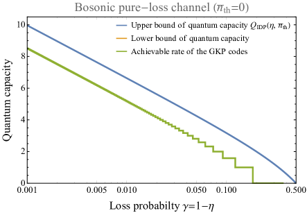
(a)

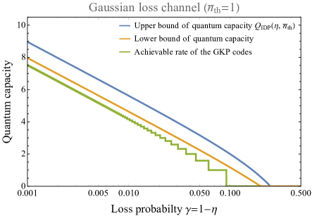
(b)

Figure 3: Achievable quantum communication rate of the GKP codes (green) compared with lower (orange) and upper (blue) bounds of quantum capacity of bosonic pure-loss channel $\mathcal{N}[\eta,\bar{n}_{\tiny\textrm{th}}=0]$ (left) and Gaussian loss channel $\mathcal{N}[\eta,\bar{n}_{\tiny\textrm{th}}=1]$ (right). Orange line in the left panel is hidden behind the blue line, since for the bosonic pure-loss channel, lower and upper bounds coincide with each other and the quantum capacity is completely known.

Note that the above estimation is overly conservative since we did not take into account the correctable displacement outside the correctable sphere. With an improved estimation of the decoding error probability, the following statement was ultimately established in Harrington and Preskill (2001):

Lemma 13 (Eq.(66) in Harrington and Preskill (2001)).

Let $\mathcal{N}_{B_{2}}[\sigma^{2}]$ be a Gaussian random displacement channel as defined in Definition 3. Also, let $\mathcal{C}_{\mathbf{S}}^{[d]}$ be the $N$-mode GKP code space defined by the stabilizers in Eq.(54). Then, there exists a symplectic lattice generated by $\mathbf{S}$ such that the GKP code achieves the following rate for the Gaussian random displacement channel $\mathcal{N}_{B_{2}}[\sigma^{2}]$ in $N\rightarrow\infty$ limit.

$$R=\max\Big{(}\log\Big{\lfloor}\frac{1}{e\sigma^{2}}\Big{\rfloor},0\Big{)}.$$ (56)

Here, $\lfloor x\rfloor$ is the floor function, due to the fact that $d$ can only be an integer.

Thus, the GKP codes achieve one-shot coherent information of the Gaussian random displacement channel (cf, Eq.(27)) in modulo floor function. Based on this, we now establish the following main result:

Theorem 14 (Achievable quantum communication rate of the GKP codes for Gaussian loss channel).

Let $\mathcal{N}[\eta,\bar{n}_{\scriptsize\textrm{th}}]$ be a Gaussian loss channel as defined in Definition 1. Upon optimal choice of $2N\times 2N$ symplectic matrix $\mathbf{S}=\mathbf{S}^{\star}$, the $N$-mode GKP code as defined in Eq.(54) achieves the following rate for the Gaussian loss channel $\mathcal{N}[\eta,\bar{n}_{\scriptsize\textrm{th}}]$ in $N\rightarrow\infty$ limit:

$$R=\max\Big{(}\log\Big{\lfloor}\frac{1}{e(1-\eta)(\bar{n}_{\scriptsize\textrm{th}}+1)}\Big{\rfloor},0\Big{)},$$ (57)

where $\lfloor x\rfloor$ is the floor function.

Proof.

Lemma 6 states that the Gaussian loss channel $\mathcal{N}[\eta,\bar{n}_{\scriptsize\textrm{th}}]$ can be converted into the Gaussian random displacement channel $\mathcal{N}_{B_{2}}[\tilde{\sigma}^{2}_{\eta,\bar{n}_{\tiny\textrm{th}}}]$ by quantum-limited amplification $\mathcal{A}[1/\eta]$, where $\tilde{\sigma}^{2}_{\eta,\bar{n}_{\tiny\textrm{th}}}=(1-\eta)(\bar{n}_{\scriptsize\textrm{th}}+1)$. Combining this with Lemma 13, Eq.(57) follows. ∎

Recall Theorem 32 and note that $Q_{\scriptsize\textrm{reg}}(\mathcal{N}[\eta,\bar{n}_{\scriptsize\textrm{th}}])\leq Q_{\scriptsize{\textrm{IDP}}}(\eta,\bar{n}_{\scriptsize\textrm{th}})$ where

$$Q_{\scriptsize{\textrm{IDP}}}(\eta,\bar{n}_{\scriptsize\textrm{th}})<\max\Big{[}\log\Big{(}\frac{1}{(1-\eta)(\bar{n}_{\scriptsize\textrm{th}}+1)}\Big{)},0\Big{]},$$ (58)

as derived from Eq.(32). Comparing this with Eq.(57), we get $Q_{\scriptsize\textrm{reg}}(\mathcal{N}[\eta,\bar{n}_{\scriptsize\textrm{th}}])-R\lesssim\log e=1.44269\cdots$, where $\sim$ is due to the floor function. Thus, GKP codes defined over optimal symplectic lattice achieve quantum capacity of Gaussian loss channels up to at most a constant gap from the upper bound of quantum capacity (see Fig. 3 for illustration).

We note that the established rate in Theorem 14 relies on the existence of a symplectic lattice in higher dimensions satisfying a certain desired condition (see Eqs.(56),(57) in Harrington and Preskill (2001)). In this regard, we remark that $E_{8}$ lattice and Leech lattice $\Lambda_{24}$ (both symplectic; see appendix of Buser and Sarnak (1994)) were recently shown to support the densest sphere packing in 8 and 24 dimensional Euclidean space, respectively Viazovska (2017); Cohn et al. (2017).

V Biconvex encoding and decoding optimization

In this subsection, we consider the energy-constrained scenario by imposing maximum allowed photon number in each mode. Instead of attempting to establish a theoretically rigorous statement as we did in the energy-unconstrained case, we tackle the problem by numerical optimization. Since decoding error probability cannot be suppressed arbitrarily close to zero with only finite number of modes, we aim to find a set of optimal encoding and decoding maps which maximize the entanglement fidelity. The main reason we chose entanglement fidelity (instead of other measures, e.g., diamond norm) as the fidelity measure is to make the optimization problem more tractable, as maximization of entanglement fidelity can be formulated as a biconvex optimization, which can be tackled by alternating semidefinite programming method.

V.1 Choi matrix and superoperator of a quantum channel

A quantum channel $\mathcal{A}:\mathcal{L}(\mathcal{H}_{1})\rightarrow\mathcal{L}(\mathcal{H}_{2})$ is a completely positive trace preserving (CPTP) map Choi (1975), which has one-to-one correspondence with the Choi matrix $\hat{X}_{\mathcal{A}}\in\mathcal{L}(\mathcal{H}_{1}\otimes\mathcal{H}_{2})$. Matrix elements of the Choi matrix are defined as $(\hat{X}_{\mathcal{A}})_{[ij],[i^{\prime}j^{\prime}]}=\langle j_{\mathcal{H}_{2}}|\mathcal{A}(|i_{\mathcal{H}_{1}}\rangle\langle i^{\prime}_{\mathcal{H}_{1}}|)|j^{\prime}_{\mathcal{H}_{2}}\rangle$, where $|i_{\mathcal{H}_{1}}\rangle,|i^{\prime}_{\mathcal{H}_{1}}\rangle$ and $|j_{\mathcal{H}_{2}}\rangle$, $|j^{\prime}_{\mathcal{H}_{2}}\rangle$ are orthonormal basis of $\mathcal{H}_{1}$ and $\mathcal{H}_{2}$, respectively. Choi matrix $\hat{X}_{\mathcal{A}}$ is hermitian positive semidefinite by definition of complete positivity (CP) of $\mathcal{A}$ Choi (1975). Also, trace preserving (TP) condition imposes the affine constraint $\textrm{Tr}_{\mathcal{H}_{2}}\hat{X}_{\mathcal{A}}\equiv\sum_{j=0}^{\scriptsize{\textrm{dim}}(\mathcal{H}_{2})-1}(X_{\mathcal{A}})_{[ij],[i^{\prime}j]}|i_{\mathcal{H}_{1}}\rangle\langle i^{\prime}_{\mathcal{H}_{1}}|=\hat{I}_{\mathcal{H}_{1}}$.

Let $\mathcal{B}:\mathcal{L}(\mathcal{H}_{2})\rightarrow\mathcal{L}(\mathcal{H}_{3})$ be another quantum channel (i.e., a CPTP map) and consider the composite channel $\mathcal{B}\cdot\mathcal{A}:\mathcal{L}(\mathcal{H}_{1})\rightarrow\mathcal{L}(\mathcal{H}_{3})$. To analyze the composite channel, it is convenient to define superoperator $\hat{T}_{\mathcal{A}}$ of a channel $\mathcal{A}$ whose matrix elements are given by $(\hat{T}_{\mathcal{A}})_{jj^{\prime},ii^{\prime}}\equiv\langle j_{\mathcal{H}_{2}}|\mathcal{A}(|i_{\mathcal{H}_{1}}\rangle\langle i^{\prime}_{\mathcal{H}_{1}}|)|j^{\prime}_{\mathcal{H}_{2}}\rangle=(\hat{X}_{\mathcal{A}})_{[ij],[i^{\prime}j^{\prime}]}$ Preskill : Superoperator of a composite channel is then given by the matrix multiplication of the superoperators of its constituting channels, i.e., $\hat{T}_{\mathcal{B}\cdot\mathcal{A}}=\hat{T}_{\mathcal{B}}\hat{T}_{\mathcal{A}}$.

V.2 Entanglement fidelity and Choi matrix

Let $\mathcal{H}_{n}$ be a Hilbert space of dimension $n$ and $\mathcal{N}:\mathcal{L}(\mathcal{H}_{n})\rightarrow\mathcal{L}(\mathcal{H}_{n})$ be a CPTP map describing a noisy quantum channel. Consider $d$-dimensional ($d\leq n$) Hilbert spaces $\mathcal{H}_{0}$ and $\mathcal{H}_{0}^{\prime}$ and assume the information sender prepared a maximally entangled state in a local noiseless memory:

$$|\Phi^{+}\rangle\equiv\frac{1}{\mathchoice{{\hbox{$\displaystyle\sqrt{d\,}$}\lower 0.4pt\hbox{\vrule height=6.94444pt,depth=-5.55559pt}}}{{\hbox{$\textstyle\sqrt{d\,}$}\lower 0.4pt\hbox{\vrule height=6.94444pt,depth=-5.55559pt}}}{{\hbox{$\scriptstyle\sqrt{d\,}$}\lower 0.4pt\hbox{\vrule height=4.8611pt,depth=-3.8889pt}}}{{\hbox{$\scriptscriptstyle\sqrt{d\,}$}\lower 0.4pt\hbox{\vrule height=3.47221pt,depth=-2.77779pt}}}}\sum_{i=0}^{d-1}|i_{\mathcal{H}_{0}}\rangle|i_{\mathcal{H}_{0}^{\prime}}\rangle.$$ (59)

The sender then encodes half of the entangled state in $\mathcal{H}_{0}$ to the channel input by a CPTP encoding map $\mathcal{E}:\mathcal{L}(\mathcal{H}_{0})\rightarrow\mathcal{L}(\mathcal{H}_{n})$, and then send it through the noisy channel $\mathcal{N}:\mathcal{L}(\mathcal{H}_{n})\rightarrow\mathcal{L}(\mathcal{H}_{n})$. The receiver then maps the received state at the channel output to the local memory by a CPTP decoding map $\mathcal{D}:\mathcal{L}(\mathcal{H}_{n})\rightarrow\mathcal{L}(\mathcal{H}_{0})$. As a result, both parties obtain an approximate entangled state

$$\hat{\rho}\equiv(\mathcal{D}\cdot\mathcal{N}\cdot\mathcal{E}\otimes\textrm{id}_{\mathcal{H}_{0}^{\prime}})(|\Phi^{+}\rangle\langle\Phi^{+}|),$$ (60)

where $\textrm{id}_{\mathcal{H}_{0}^{\prime}}:\mathcal{L}(\mathcal{H}_{0}^{\prime})\rightarrow\mathcal{L}(\mathcal{H}_{0}^{\prime})$ is the identity map associated with the noiseless local memory at the sender’s side. Note that $\hat{\rho}$ in Eq.(60) is explicitly given by

$$\hat{\rho}=\frac{1}{d}\sum_{i,i^{\prime}=0}^{d-1}(\hat{X}_{\mathcal{D}\cdot\mathcal{N}\cdot\mathcal{E}})_{[ij],[i^{\prime}j^{\prime}]}|j_{\mathcal{H}_{0}}\rangle\langle j^{\prime}_{\mathcal{H}_{0}}|\otimes|i_{\mathcal{H}_{0}^{\prime}}\rangle\langle i^{\prime}_{\mathcal{H}_{0}^{\prime}}|,$$ (61)

where $\hat{X}_{\mathcal{D}\cdot\mathcal{N}\cdot\mathcal{E}}\in\mathcal{L}(\mathcal{H}_{0}\otimes\mathcal{H}_{0})$ is the Choi matrix of the composite channel $\mathcal{D}\cdot\mathcal{N}\cdot\mathcal{E}$. Thus, $\hat{\rho}$ is isomorphic to the Choi matrix $\hat{X}_{\mathcal{D}\cdot\mathcal{N}\cdot\mathcal{E}}$.

Quality of the approximate non-local entangled state $\hat{\rho}$ can be measured by the entanglement fidelity $F_{e}(\hat{\rho})\equiv\langle\Phi^{+}|\hat{\rho}|\Phi^{+}\rangle$ Schumacher (1996), where $F_{e}(\hat{\rho})=1$ iff $\hat{\rho}$ is a noiseless maximally entangled state $|\Phi^{+}\rangle\langle\Phi^{+}|$. Isomorphism between $\hat{\rho}$ and $\hat{X}_{\mathcal{D}\cdot\mathcal{N}\cdot\mathcal{E}}$ then yields

$$F_{e}(\hat{\rho})=(1/d^{2})\sum_{i,i^{\prime}=0}^{d-1}(\hat{X}_{\mathcal{D}\cdot\mathcal{N}\cdot\mathcal{E}})_{[ii],[i^{\prime}i^{\prime}]}=\frac{1}{d^{2}}\textrm{Tr}[\hat{T}_{\mathcal{D}\cdot\mathcal{N}\cdot\mathcal{E}}],$$ (62)

where $\hat{T}_{\mathcal{D}\cdot\mathcal{N}\cdot\mathcal{E}}$ is the superoperator of $\mathcal{D}\cdot\mathcal{N}\cdot\mathcal{E}$. Note that $\hat{T}_{\mathcal{D}\cdot\mathcal{N}\cdot\mathcal{E}}=\hat{T}_{\mathcal{D}}\hat{T}_{\mathcal{N}}\hat{T}_{\mathcal{E}}$ can be decomposed as

$$(\hat{T}_{\mathcal{D}\cdot\mathcal{N}\cdot\mathcal{E}})_{jj^{\prime},ii^{\prime}}$$

$$\,\,\,=\sum_{k,k^{\prime},l,l^{\prime}=0}^{n-1}(\hat{X}_{\mathcal{D}})_{[lj],[l^{\prime}j^{\prime}]}(\hat{X}_{\mathcal{N}})_{[kl],[k^{\prime}l^{\prime}]}(\hat{X}_{\mathcal{E}})_{[ik],[i^{\prime}k^{\prime}]},$$ (63)

where $\hat{X}_{\mathcal{D}}\in\mathcal{L}(\mathcal{H}_{0}\otimes\mathcal{H}_{n})$, $\hat{X}_{\mathcal{N}}\in\mathcal{L}(\mathcal{H}_{n}\otimes\mathcal{H}_{n})$ and $\hat{X}_{\mathcal{E}}\in\mathcal{L}(\mathcal{H}_{n}\otimes\mathcal{H}_{0})$ are the Choi matrices of decoding, noisy channel, and encoding, respectively, and $i,i^{\prime},j,j^{\prime}\in\{0,\cdots,d-1\}$. We note that the entanglement fidelity $F_{e}(\hat{\rho})$ is a bi-linear function of $\hat{X}_{\mathcal{E}}$ and $\hat{X}_{\mathcal{E}}$, since $\hat{T}_{\mathcal{D}\cdot\mathcal{N}\cdot\mathcal{E}}$ is bi-linear in $\hat{X}_{\mathcal{E}}$ and $\hat{X}_{\mathcal{E}}$, as can be seen from Eq.(63).

To make the bi-linearity more evident, we define a linear map $f_{\mathcal{N}}:\mathcal{L}(\mathcal{H}_{n}\otimes\mathcal{H}_{0})\rightarrow\mathcal{L}(\mathcal{H}_{0}\otimes\mathcal{H}_{n})$ such that

$$\big{(}f_{\mathcal{N}}(\hat{X})\big{)}_{[l^{\prime}i^{\prime}],[li]}\equiv\sum_{k,k^{\prime}=0}^{n-1}(\hat{X}_{\mathcal{N}})_{[kl],[k^{\prime}l^{\prime}]}(\hat{X})_{[ik],[i^{\prime}k^{\prime}]},$$ (64)

where $l,l^{\prime}\in\{0,\cdots,n-1\}$. Entanglement fidelity $F_{e}(\hat{\rho})$ is then given by

$$F_{e}(\hat{\rho})=\frac{1}{d^{2}}\textrm{Tr}\Big{[}\hat{X}_{\mathcal{D}}f_{\mathcal{N}}(\hat{X}_{\mathcal{E}})\Big{]},$$ (65)

which is apparently bi-linear in $\hat{X}_{\mathcal{E}}$ and $\hat{X}_{\mathcal{D}}$.

V.3 Maximization of entanglement fidelity

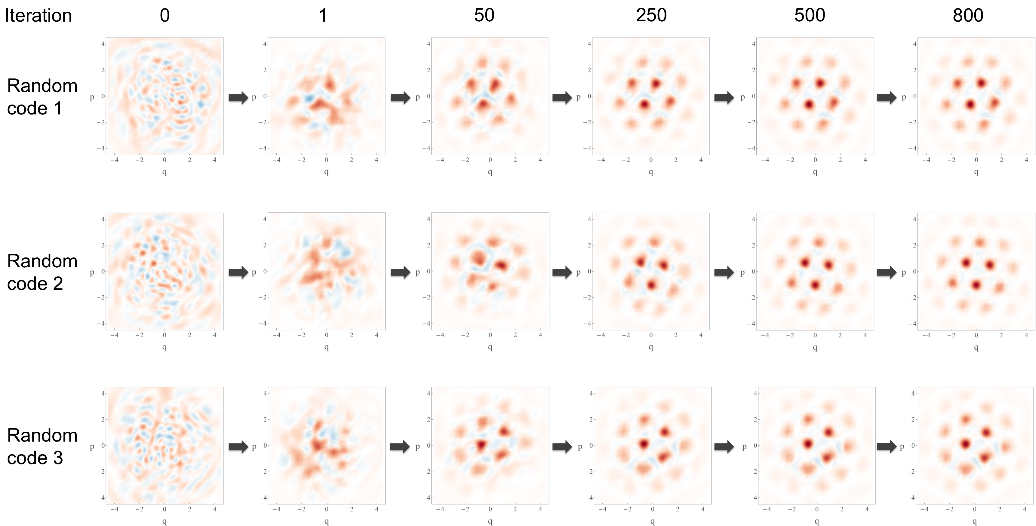
Figure 4: Biconvex optimization of the encoding and decoding maps for bosonic pure-loss channel $\mathcal{N}[\eta,0]$ with $\eta=0.9$. We chose $n=20$ and $d=2$ and imposed photon number constraint $\textrm{Tr}[\hat{n}\hat{\rho}_{\mathcal{E}}]\leq\ 3$, where $\hat{\rho}_{\mathcal{E}}=(1/d)\textrm{Tr}_{\mathcal{H}_{0}}\hat{X}_{\mathcal{E}}$ is the maximally mixed code state. First column of each row is the Wigner function of $\hat{\rho}_{\mathcal{E}}$ for a randomly generated encoding map $\mathcal{E}$. From the second to the sixth columns represent the updated code spaces after $1,50,250,500$ and $800$ iterations of alternating semidefinite programming. Color scale is the same as in Fig. 2.

It is known that finding optimal decoding operation which maximizes the entanglement fidelity is a semidefinite programming, if the encoding map is fixed to $\mathcal{E}=\bar{\mathcal{E}}$ Reimpell and Werner (2005); Fletcher et al. (2007):

$$\max_{\hat{X}_{\mathcal{D}}} \textrm{Tr}[\hat{X}_{\mathcal{D}}(f_{\mathcal{N}}(\hat{X}_{\bar{\mathcal{E}}}))]$$

s.t. $$\hat{X}_{\mathcal{D}}=\hat{X}_{\mathcal{D}}^{\dagger}\succeq 0,\,\,\textrm{Tr}_{\mathcal{H}_{0}}\hat{X}_{\mathcal{D}}=\hat{I}_{\mathcal{H}_{n}},$$ (66)

where the constrains are due to the CPTP nature of $\mathcal{D}$. Similarly, optimizing encoding while fixing decoding is also a semidefinite programming, and thus the entire problem is a biconvex optimization Kosut and Lidar (2009). Here, we further impose an energy constraint to the encoding map while still preserving bi-convexity of the problem. Let $\hat{E}\in\mathcal{L}(\mathcal{H}_{n})$ be an energy observable. We define $\textrm{Tr}_{\mathcal{H}_{n}}[\hat{E}\hat{\rho}_{\mathcal{E}}]$ to be the average energy in the encoded state, where $\hat{\rho}_{\mathcal{E}}\equiv\mathcal{E}(\frac{1}{d}\sum_{i=0}^{d-1}|i_{\mathcal{H}_{0}}\rangle\langle i_{\mathcal{H}_{0}}|)=\frac{1}{d}\textrm{Tr}_{\mathcal{H}_{0}}\hat{X}_{\mathcal{E}}$ is the maximally mixed encoded state. Then, the energy constraint reads $\textrm{Tr}[(\hat{E}\otimes\hat{I}_{\mathcal{H}_{0}})\hat{X}_{\mathcal{E}}]\leq\bar{E}d$ and we obtain the following biconvex encoding and decoding optimization with energy constraint:

$$\max_{\hat{X}_{\mathcal{E}},\hat{X}_{\mathcal{D}}} \textrm{Tr}[\hat{X}_{\mathcal{D}}^{\dagger}f_{\mathcal{N}}(\hat{X}_{\mathcal{E}})],\,\,$$

s.t. $$\hat{X}_{\mathcal{D}}=\hat{X}_{\mathcal{D}}^{\dagger}\succeq 0,\,\,\textrm{Tr}_{\mathcal{H}_{0}}\hat{X}_{\mathcal{D}}=\hat{I}_{\mathcal{H}_{n}},$$

$$\hat{X}_{\mathcal{E}}=\hat{X}_{\mathcal{E}}^{\dagger}\succeq 0,\,\,\textrm{Tr}_{\mathcal{H}_{n}}\hat{X}_{\mathcal{E}}=\hat{I}_{\mathcal{H}_{0}},$$

$$\quad\textrm{and}\,\,\textrm{Tr}[(\hat{E}\otimes\hat{I}_{\mathcal{H}_{0}})\hat{X}_{\mathcal{E}}]\leq\bar{E}d,$$ (67)

where the second line in the constraint is due to the CPTP nature of the encoding map $\mathcal{E}$, and the third line is due to the encoding energy constraint.

We apply Eq.(67) to find an optimal qubit-into-oscillator encoding (i.e., $\textrm{dim}(\mathcal{H}_{0})=d=2$) against the bosonic pure-loss channel $\mathcal{N}[\eta,0]$ subject to the photon number constraint $\textrm{Tr}[\hat{n}\hat{\rho}_{\mathcal{E}}]\leq\bar{n}$. For practical implementation, since the photon number cannot increase under the bosonic pure-loss channel, we confine the bosonic Hilbert space to a truncated subspace $\mathcal{H}_{n}\equiv\textrm{span}\{|0\rangle,\cdots,|n-1\rangle\}$, yielding $\mathcal{N}(\hat{\rho})=\mathcal{N}[\eta,0](\hat{\rho})=\sum_{\ell=0}^{n-1}\hat{E}_{\ell}\hat{\rho}\hat{E}_{\ell}^{\dagger}$ where $\hat{E}_{\ell}=\mathchoice{{\hbox{$\displaystyle\sqrt{(1-\eta)^{\ell}/\ell!\,}$}\lower 0.4pt\hbox{\vrule height=9.44444pt,depth=-7.55559pt}}}{{\hbox{$\textstyle\sqrt{(1-\eta)^{\ell}/\ell!\,}$}\lower 0.4pt\hbox{\vrule height=9.44444pt,depth=-7.55559pt}}}{{\hbox{$\scriptstyle\sqrt{(1-\eta)^{\ell}/\ell!\,}$}\lower 0.4pt\hbox{\vrule height=6.63889pt,depth=-5.31114pt}}}{{\hbox{$\scriptscriptstyle\sqrt{(1-\eta)^{\ell}/\ell!\,}$}\lower 0.4pt\hbox{\vrule height=5.13889pt,depth=-4.11113pt}}}\eta^{\frac{\hat{n}}{2}}\hat{a}^{\ell}$. We choose $n\gg\bar{n}$ to avoid artifacts caused by truncation and solve Eq.(67) heuristically by alternating encoding and decoding optimization, each solved by semidefinite programming, starting from a random initial encoding map. We generate random initial codes by taking the first $d$ columns of a Haar random $n\times n$ unitary matrix. To solve each SDP sub-problem we used CVX, a package for specifying and solving convex programs CVX Research (2012); Grant and Boyd (2008).

In Fig. 4, we took $\eta=0.9$, $n=20$, $d=2$ and $\bar{n}=3$ and plot the Wigner function of maximally mixed code states of the numerically optimized codes (last column), starting from three different random initial encoding maps (first column). In all instances, the obtained codes are similar to the hexagonal GKP code (in Fig. 2), except an overall displacement. We note that the optimized code in second row exhibits the best performance (i.e., $1-F_{\mathcal{N}}^{\star}=0.002092$) among all. Although we do not attempt to make a rigorous claim, this might indicate that the GKP codes defined over the symplectic lattice allowing the most efficient sphere packing may be the optimal encoding for the Gaussian loss channels. In particular, the constant gap in Theorem 14 may be closed if we assume the optimal decoding, instead of the sub-optimal one involving (noisy) quantum-limited amplification, which we assumed to prove Eq.(57).

We emphasize that the biconvex optimization in Eq.(67) explores the most general form of encoding maps, including the mixed state encoding. From the numerical optimization, however, we only obtained pure-state encoding (i.e., $\mathcal{E}(\hat{\rho}_{0})=\hat{V}\hat{\rho}_{0}\hat{V}^{\dagger}$, where $\hat{V}:\mathcal{H}_{0}\rightarrow\mathcal{H}_{n}$ is an isometry $\hat{V}^{\dagger}\hat{V}=\hat{I}_{\mathcal{H}_{0}}$) as an optimal solution at all iterations of SDP sub-problem. We also stress that the alternating semidefinite programming method is not guaranteed to yield a global optimal solution, although the obtained hexagonal GKP code in Fig. 4 may be a global optimum. In principle, global optimal solution of Eq.(67) can be deterministically found by global optimization algorithm outlined in Floudas and Visweswaran (1990). To implement the algorithm, however, one should in general solve exponentially many convex sub-problems in the number of complicating variables (responsible for non-convexity of the problem; see Floudas and Visweswaran (1990) for details), which is intractable in our application.

VI Conclusion

Exploiting various synthesis and decomposition of Gaussian channels, we provided improved upper bounds on the Gaussian thermal loss channel, both in the energy constrained and unconstrained cases, and the Gaussian displacement channel (Theorems 32, 11, 12 and Eq.(42)). We also established an achievable rate of the GKP codes for the Gaussian loss channels (Theorem 14). In the energy-unconstrained case, in particular, we showed that the GKP codes achieve the upper bound of Gaussian loss channel capacity upto at most a constant gap $\simeq\log e=1.44269\cdots$ in the unit of qubits per channel use. In the energy-constrained case, we formulated a biconvex encoding and decoding optimization problem and solved it via alternating semidefinite programming method. We demonstrated in the one-mode case that hexagonal GKP code emerges as an optimal encoding from Haar random initial codes.

As was proven in Barnum and Knill (2002), entanglement infidelity of the Petz decoding Petz (1986, 1988) (or, transpose decoding) is at most twice as large as the optimal entanglement infidelity. Thus, communication rate achievable by Petz decoding equals to the optimal achievable rate. We leave finding the optimal communication rate of the GKP codes for Gaussian loss channels as an open problem.

Note added: While preparing the manuscript, we became aware of a related work Rosati et al. (2018) in which Lemma 8 and Theorem 32 were independently discovered. We also realized our Theorem 11 was independently discovered in Sharma et al. (2017). We thank the authors of Sharma et al. (2017) for pointing out a mistake we made in Eq.(35) in an earlier version of our manuscript.

Appendix A Bosonic mode, Gaussian states and Gaussian unitary operations

Let $\mathcal{H}$ denote an infinite-dimensional Hilbert space. Quantum states of $N$ bosonic modes are in the tensor product of $N$ such Hilbert spaces $\mathcal{H}^{\otimes N}$. Each bosonic mode is associated with the annihilation and creation operators $\hat{a}_{k}$ and $\hat{a}^{\dagger}_{k}$, satisfying the bosonic communication relation $[\hat{a}_{i},\hat{a}_{j}]=[\hat{a}^{\dagger}_{i},\hat{a}^{\dagger}_{j}]=0$, $[\hat{a}_{i},\hat{a}^{\dagger}_{j}]=\delta_{ij}$, where $\delta_{ij}$ is the Kronecker delta function and $[\hat{A},\hat{B}]\equiv\hat{A}\hat{B}-\hat{B}\hat{A}$. Hilbert space $\mathcal{H}$ is spanned by the eigenstates of the number operator $\hat{n}\equiv\hat{a}^{\dagger}\hat{a}$, i.e., $\mathcal{H}=\textrm{span}\{|n\rangle\}_{n=0}^{\infty}$ where $\hat{n}|n\rangle=n|n\rangle$. In the number basis (or Fock basis), annihilation and creation operators are given by $\hat{a}=\sum_{n=1}^{\infty}\mathchoice{{\hbox{$\displaystyle\sqrt{n\,}$}\lower 0.4pt\hbox{\vrule height=4.30554pt,depth=-3.44446pt}}}{{\hbox{$\textstyle\sqrt{n\,}$}\lower 0.4pt\hbox{\vrule height=4.30554pt,depth=-3.44446pt}}}{{\hbox{$\scriptstyle\sqrt{n\,}$}\lower 0.4pt\hbox{\vrule height=3.01389pt,depth=-2.41113pt}}}{{\hbox{$\scriptscriptstyle\sqrt{n\,}$}\lower 0.4pt\hbox{\vrule height=2.15277pt,depth=-1.72223pt}}}|n-1\rangle\langle n|$, $\hat{a}^{\dagger}=\sum_{n=0}^{\infty}\mathchoice{{\hbox{$\displaystyle\sqrt{n+1\,}$}\lower 0.4pt\hbox{\vrule height=6.44444pt,depth=-5.15558pt}}}{{\hbox{$\textstyle\sqrt{n+1\,}$}\lower 0.4pt\hbox{\vrule height=6.44444pt,depth=-5.15558pt}}}{{\hbox{$\scriptstyle\sqrt{n+1\,}$}\lower 0.4pt\hbox{\vrule height=4.51111pt,depth=-3.6089pt}}}{{\hbox{$\scriptscriptstyle\sqrt{n+1\,}$}\lower 0.4pt\hbox{\vrule height=3.22221pt,depth=-2.57779pt}}}|n+1\rangle\langle n|$. Coherent state $|\alpha\rangle$ is an eigenstate of the annihilation operator $\hat{a}$ with eigenvalue $\alpha$, i.e., $\hat{a}|\alpha\rangle=\alpha|\alpha\rangle$. In the Fock basis, $|\alpha\rangle$ is given by $|\alpha\rangle=e^{-\frac{1}{2}|\alpha|^{2}}\sum_{n=0}^{\infty}\frac{\alpha^{n}}{\mathchoice{{\hbox{$\displaystyle\sqrt{n!\,}$}\lower 0.4pt\hbox{\vrule height=4.8611pt,depth=-3.8889pt}}}{{\hbox{$\textstyle\sqrt{n!\,}$}\lower 0.4pt\hbox{\vrule height=4.8611pt,depth=-3.8889pt}}}{{\hbox{$\scriptstyle\sqrt{n!\,}$}\lower 0.4pt\hbox{\vrule height=3.40277pt,depth=-2.72223pt}}}{{\hbox{$\scriptscriptstyle\sqrt{n!\,}$}\lower 0.4pt\hbox{\vrule height=2.43054pt,depth=-1.94444pt}}}}|n\rangle$. Note that the vacuum state $|0\rangle$ is a special case of coherent state with $\alpha=0$. Displacement operator $\hat{D}(\alpha)$ is defined as $\hat{D}(\alpha)\equiv\exp(\alpha\hat{a}^{\dagger}-\alpha^{*}\hat{a})$. Coherent state $|\alpha\rangle$ is a displaced vacuum state:

$$|\alpha\rangle=\hat{D}(\alpha)|0\rangle.$$ (68)

Quadrature operators are defined as $\hat{q}_{k}\equiv\frac{1}{\mathchoice{{\hbox{$\displaystyle\sqrt{2\,}$}\lower 0.4pt\hbox{\vrule height=4.51111pt,depth=-3.6089pt}}}{{\hbox{$\textstyle\sqrt{2\,}$}\lower 0.4pt\hbox{\vrule height=4.51111pt,depth=-3.6089pt}}}{{\hbox{$\scriptstyle\sqrt{2\,}$}\lower 0.4pt\hbox{\vrule height=3.15778pt,depth=-2.52625pt}}}{{\hbox{$\scriptscriptstyle\sqrt{2\,}$}\lower 0.4pt\hbox{\vrule height=2.25555pt,depth=-1.80446pt}}}}(\hat{a}_{k}+\hat{a}_{k}^{\dagger})$, $\hat{p}_{k}\equiv\frac{i}{\mathchoice{{\hbox{$\displaystyle\sqrt{2\,}$}\lower 0.4pt\hbox{\vrule height=4.51111pt,depth=-3.6089pt}}}{{\hbox{$\textstyle\sqrt{2\,}$}\lower 0.4pt\hbox{\vrule height=4.51111pt,depth=-3.6089pt}}}{{\hbox{$\scriptstyle\sqrt{2\,}$}\lower 0.4pt\hbox{\vrule height=3.15778pt,depth=-2.52625pt}}}{{\hbox{$\scriptscriptstyle\sqrt{2\,}$}\lower 0.4pt\hbox{\vrule height=2.25555pt,depth=-1.80446pt}}}}(\hat{a}_{k}^{\dagger}-\hat{a}_{k})$ and are called position and momentum operator, respectively. We follow the same convention as used for the GKP codes Gottesman et al. (2001); Albert et al. (2017) which differs from Ref. Weedbrook et al. (2012) by a factor of $\textstyle\sqrt{2\,}$  in the definition of $\hat{q}_{k}$ and $\hat{p}_{k}$. Define $\mathbf{\hat{x}}\equiv(\hat{q}_{1},\hat{p}_{1},\cdots,\hat{q}_{N},\hat{p}_{N})^{T}$. Then, the bosonic commutation relation reads $[\hat{x}_{i},\hat{x}_{j}]=i\Omega_{ij}$, where $\mathbf{\Omega}$ is defined as

$$\mathbf{\Omega}\equiv\begin{pmatrix}\mathbf{\omega}&&\\ &\ddots&\\ &&\mathbf{\omega}\end{pmatrix}\textrm{ and }\mathbf{\omega}\equiv\begin{pmatrix}0&1\\ -1&0\end{pmatrix}.$$ (69)

Eigenvalue spectrum of quadrature operators are continuous, $\hat{q}|q\rangle=q|q\rangle,\quad\hat{p}|p\rangle=p|p\rangle$, where $q,p\in(-\infty,\infty)$ and the eigenstates are normalized by the Dirac delta function: $\langle q|q^{\prime}\rangle=\delta(q-q^{\prime})$ and $\langle p|p^{\prime}\rangle=\delta(p-p^{\prime})$. Also, $|q\rangle$ and $|p\rangle$ are related by Fourier transformation $|q\rangle=\frac{1}{\mathchoice{{\hbox{$\displaystyle\sqrt{2\pi\,}$}\lower 0.4pt\hbox{\vrule height=4.51111pt,depth=-3.6089pt}}}{{\hbox{$\textstyle\sqrt{2\pi\,}$}\lower 0.4pt\hbox{\vrule height=4.51111pt,depth=-3.6089pt}}}{{\hbox{$\scriptstyle\sqrt{2\pi\,}$}\lower 0.4pt\hbox{\vrule height=3.15778pt,depth=-2.52625pt}}}{{\hbox{$\scriptscriptstyle\sqrt{2\pi\,}$}\lower 0.4pt\hbox{\vrule height=2.25555pt,depth=-1.80446pt}}}}\int_{-\infty}^{\infty}dpe^{-iqp}|p\rangle$, $|p\rangle=\frac{1}{\mathchoice{{\hbox{$\displaystyle\sqrt{2\pi\,}$}\lower 0.4pt\hbox{\vrule height=4.51111pt,depth=-3.6089pt}}}{{\hbox{$\textstyle\sqrt{2\pi\,}$}\lower 0.4pt\hbox{\vrule height=4.51111pt,depth=-3.6089pt}}}{{\hbox{$\scriptstyle\sqrt{2\pi\,}$}\lower 0.4pt\hbox{\vrule height=3.15778pt,depth=-2.52625pt}}}{{\hbox{$\scriptscriptstyle\sqrt{2\pi\,}$}\lower 0.4pt\hbox{\vrule height=2.25555pt,depth=-1.80446pt}}}}\int_{-\infty}^{\infty}dpe^{iqp}|q\rangle$. Upon displacement,

$$\hat{D}(\xi_{1}/\mathchoice{{\hbox{$\displaystyle\sqrt{2\,}$}\lower 0.4pt\hbox{\vrule height=6.44444pt,depth=-5.15558pt}}}{{\hbox{$\textstyle\sqrt{2\,}$}\lower 0.4pt\hbox{\vrule height=6.44444pt,depth=-5.15558pt}}}{{\hbox{$\scriptstyle\sqrt{2\,}$}\lower 0.4pt\hbox{\vrule height=4.51111pt,depth=-3.6089pt}}}{{\hbox{$\scriptscriptstyle\sqrt{2\,}$}\lower 0.4pt\hbox{\vrule height=3.22221pt,depth=-2.57779pt}}})|q\rangle =e^{-i\xi_{1}\hat{p}}|q\rangle\, =|q+\xi_{1}\rangle,$$

$$\hat{D}(i\xi_{2}/\mathchoice{{\hbox{$\displaystyle\sqrt{2\,}$}\lower 0.4pt\hbox{\vrule height=6.44444pt,depth=-5.15558pt}}}{{\hbox{$\textstyle\sqrt{2\,}$}\lower 0.4pt\hbox{\vrule height=6.44444pt,depth=-5.15558pt}}}{{\hbox{$\scriptstyle\sqrt{2\,}$}\lower 0.4pt\hbox{\vrule height=4.51111pt,depth=-3.6089pt}}}{{\hbox{$\scriptscriptstyle\sqrt{2\,}$}\lower 0.4pt\hbox{\vrule height=3.22221pt,depth=-2.57779pt}}})|p\rangle =e^{i\xi_{2}\hat{q}}|p\rangle =|p+\xi_{2}\rangle.$$ (70)

Let $\mathcal{L}(\mathcal{H})$ be the space of linear operators on the Hilbert space $\mathcal{H}$. General quantum states (including mixed states) are described by density operator $\hat{\rho}\in\mathcal{D}(\mathcal{H})$, where $\mathcal{D}(\mathcal{H})\equiv\{\hat{\rho}\in\mathcal{L}(\mathcal{H})\,|\,\hat{\rho}^{\dagger}=\hat{\rho}\succeq 0,\textrm{Tr}[\hat{\rho}]=1\}$. Expectation value of an observable $\hat{E}$ of the state $\hat{\rho}$ is given by $\langle\hat{E}\rangle=\textrm{Tr}[\hat{\rho}\hat{E}]$. Wigner characteristic function $\chi(\mathbf{\xi})$ is defined as $\chi(\mathbf{\xi})\equiv\textrm{Tr}[\hat{\rho}\exp(i\mathbf{\hat{x}}^{T}\mathbf{\Omega}\mathbf{\xi})]$, where $\hat{\rho}\in\mathcal{D}(\mathcal{H}^{\otimes N})$ and $\mathbf{\xi}=(\xi_{1},\cdots,\xi_{2N})^{T}$. Weyl operator $\exp(i\mathbf{\hat{x}}^{T}\mathbf{\Omega}\mathbf{\xi})$ is of the form of displacement operator and satisfies the orthogonality relation $\textrm{Tr}[\exp(-i\mathbf{\hat{x}}^{T}\mathbf{\Omega}\mathbf{\xi})\exp(i\mathbf{\hat{x}}^{T}\mathbf{\Omega}\mathbf{\xi^{\prime}})]=(2\pi)^{N}\delta(\mathbf{\xi}-\mathbf{\xi^{\prime}})$. Wigner characteristic function $\chi(\mathbf{\xi})$ is in one-to-one correspondence with the state $\hat{\rho}$ and the inverse function is given by $\hat{\rho}=\frac{1}{(2\pi)^{N}}\int d^{2N}\mathbf{\xi}\chi(\mathbf{\xi})\exp(-i\mathbf{\hat{x}}^{T}\mathbf{\Omega}\mathbf{\xi})$. Wigner function $W(\mathbf{x})$ is Fourier transformation of $\chi(\mathbf{\xi})$, i.e.,

$$W(\mathbf{x})=\frac{1}{(2\pi)^{N}}\int d^{2N}\mathbf{\xi}\chi(\mathbf{\xi})\exp(-i\mathbf{x}^{T}\mathbf{\Omega}\mathbf{\xi}),$$ (71)

where $\mathbf{x}=(x_{1},\cdots,x_{N})^{T}$ is the eigenvalue of the quadrature operator $\mathbf{\hat{x}}$.

A quantum state $\hat{\rho}$ is Gaussian iff its Wigner characteristic function and Wigner function are Gaussian Weedbrook et al. (2012):

$$\chi(\mathbf{\xi}) =\exp\big{[}-\frac{1}{2}\mathbf{\xi}^{T}(\mathbf{\Omega}\mathbf{V}\mathbf{\Omega}^{T})\mathbf{\xi}-i(\mathbf{\Omega}\mathbf{\bar{x}})\mathbf{\xi}\big{]},$$

$$W(\mathbf{x}) =\frac{\exp\big{[}-\frac{1}{2}(\mathbf{x}-\mathbf{\bar{x}})^{T}\mathbf{V}^{-1}(\mathbf{x}-\mathbf{\bar{x}})\big{]}}{(2\pi)^{N}\mathchoice{{\hbox{$\displaystyle\sqrt{\textrm{det}\mathbf{V}\,}$}\lower 0.4pt\hbox{\vrule height=6.94444pt,depth=-5.55559pt}}}{{\hbox{$\textstyle\sqrt{\textrm{det}\mathbf{V}\,}$}\lower 0.4pt\hbox{\vrule height=6.94444pt,depth=-5.55559pt}}}{{\hbox{$\scriptstyle\sqrt{\textrm{det}\mathbf{V}\,}$}\lower 0.4pt\hbox{\vrule height=4.8611pt,depth=-3.8889pt}}}{{\hbox{$\scriptscriptstyle\sqrt{\textrm{det}\mathbf{V}\,}$}\lower 0.4pt\hbox{\vrule height=3.47221pt,depth=-2.77779pt}}}},$$ (72)

where $\mathbf{\bar{x}},\mathbf{V}$ are first and second moments of the state $\hat{\rho}$.

$$\mathbf{\bar{x}}\equiv\langle\mathbf{\hat{x}}\rangle=\textrm{Tr}[\hat{\rho}\mathbf{\hat{x}}],\quad V_{ij}\equiv\frac{1}{2}\langle\{\hat{x}_{i}-\bar{x}_{i},\hat{x}_{j}-\bar{x}_{j}\}\rangle,$$ (73)

where $\{\hat{A},\hat{B}\}\equiv\hat{A}\hat{B}+\hat{B}\hat{A}$. Thus, Gaussian states are fully characterized by the first two moments, i.e., $\hat{\rho}=\hat{\rho}_{G}(\mathbf{\bar{x}},\mathbf{V})$. Heisenberg uncertainty relation reads $\mathbf{V}+\frac{i}{2}\mathbf{\Omega}\succeq 0$ and implies $V(\hat{q}_{k})V(\hat{p}_{k})\geq\frac{1}{4}$ for all $k\in\{1,\cdots,N\}$, where $V(\hat{x}_{i})\equiv\mathbf{V}_{ii}$.

Vacuum state $|0\rangle\langle 0|$ is the simplest example of one-mode Gaussian states with $\mathbf{\bar{x}}=\mathbf{0}$ and $\mathbf{V}=\frac{\mathbf{I}_{2}}{2}$, where $\mathbf{I}_{n}$ is defined as the $n\times n$ identity matrix. Coherent state $|\alpha\rangle\langle\alpha|$ is also Gaussian: $|\alpha\rangle\langle\alpha|=\hat{\rho}_{G}(\mathbf{\bar{x}}_{\alpha},\frac{\mathbf{I}_{2}}{2})$ with $\mathbf{\bar{x}}_{\alpha}\equiv\mathchoice{{\hbox{$\displaystyle\sqrt{2\,}$}\lower 0.4pt\hbox{\vrule height=6.44444pt,depth=-5.15558pt}}}{{\hbox{$\textstyle\sqrt{2\,}$}\lower 0.4pt\hbox{\vrule height=6.44444pt,depth=-5.15558pt}}}{{\hbox{$\scriptstyle\sqrt{2\,}$}\lower 0.4pt\hbox{\vrule height=4.51111pt,depth=-3.6089pt}}}{{\hbox{$\scriptscriptstyle\sqrt{2\,}$}\lower 0.4pt\hbox{\vrule height=3.22221pt,depth=-2.57779pt}}}(\alpha_{R},\alpha_{I})^{T}$ and $\alpha=\alpha_{R}+i\alpha_{I}$. Coherent states (including the vacuum state) saturate the uncertainty inequality and thus have the minimum uncertainty. Thermal state is an example of Gaussian mixed states and is given by

$$\hat{\rho}_{\bar{n}_{\tiny\textrm{th}}}\equiv\sum_{n=0}^{\infty}\frac{(\bar{n}_{\scriptsize\textrm{th}})^{n}}{(\bar{n}_{\scriptsize\textrm{th}}+1)^{n+1}}|n\rangle\langle n|=\hat{\rho}_{G}(\mathbf{0},(\bar{n}_{\scriptsize\textrm{th}}+\frac{1}{2})\mathbf{I}_{2}),$$ (74)

in the Fock basis, where $\bar{n}_{\scriptsize\textrm{th}}$ is the average photon number, i.e., $\bar{n}_{\scriptsize\textrm{th}}=\textrm{Tr}[\hat{\rho}_{\bar{n}_{\tiny\textrm{th}}}\hat{n}]$. Quantum entropy of a state $\hat{\rho}$ is defined as $H(\hat{\rho})\equiv-\textrm{Tr}[\hat{\rho}\log\hat{\rho}]$, where $\log$ is the logarithm with base $2$. Entropy of a thermal state $\hat{\rho}_{\bar{n}_{\tiny\textrm{th}}}$ is given by

$$H(\hat{\rho}_{\bar{n}_{\tiny\textrm{th}}})=g(\bar{n}_{\scriptsize\textrm{th}}),$$ (75)

where $g(x)\equiv(x+1)\log(x+1)-x\log x$. Since thermal state is a mixed state, $H(\hat{\rho}_{\bar{n}_{\tiny\textrm{th}}})\geq 0$ where the equality holds only when the state is vacuum, i.e., $\bar{n}_{\scriptsize\textrm{th}}=0$.

Unitary operations that map a Gaussian state to another Gaussian state are called Gaussian unitary operations. Gaussian unitaries are generated by second order polynomials of $\mathbf{\hat{a}}=(\hat{a}_{1},\cdots,\hat{a}_{N})^{T}$ and $\mathbf{\hat{a}^{\dagger}}=(\hat{a}_{1}^{\dagger},\cdots,\hat{a}_{N}^{\dagger})^{T}$, i.e., $\hat{U}_{G}=\exp(-i\hat{H})$ with $\hat{H}=i(\mathbf{\alpha}^{T}\mathbf{\hat{a}^{\dagger}}+\mathbf{\hat{a}^{\dagger}}\mathbf{F}\mathbf{\hat{a}}+\mathbf{\hat{a}^{\dagger}}\mathbf{G}\mathbf{\hat{a}^{\dagger}})+\textrm{h.c.}$, where $\mathbf{\alpha}^{T}=(\alpha_{1},\cdots,\alpha_{N})$ and $\mathbf{F},\mathbf{G}$ are $N\times N$ complex matrices. In the Heisenberg picture, annihilation operator $\mathbf{\hat{a}}$ is transformed into $\hat{U}_{G}^{\dagger}\mathbf{\hat{a}}\hat{U}_{G}=\mathbf{A}\mathbf{\hat{a}}+\mathbf{B}\mathbf{\hat{a}^{\dagger}}+\mathbf{\alpha}$, where $N\times N$ complex matrices $\mathbf{A},\mathbf{B}$ (determined by $\mathbf{F},\mathbf{G}$) satisfy $\mathbf{A}\mathbf{B}^{T}=\mathbf{B}\mathbf{A}^{T}$ and $\mathbf{A}\mathbf{A}^{\dagger}=\mathbf{B}\mathbf{B}^{\dagger}+\mathbf{I}_{N}$. In terms of quadrature operators, the transformation reads $\mathbf{x}\rightarrow\hat{U}_{G}^{\dagger}\mathbf{x}\hat{U}_{G}=\mathbf{S}\mathbf{x}+\mathbf{d}$, where $\mathbf{d}=(d_{1},\cdots,d_{2N})^{T}=\mathchoice{{\hbox{$\displaystyle\sqrt{2\,}$}\lower 0.4pt\hbox{\vrule height=6.44444pt,depth=-5.15558pt}}}{{\hbox{$\textstyle\sqrt{2\,}$}\lower 0.4pt\hbox{\vrule height=6.44444pt,depth=-5.15558pt}}}{{\hbox{$\scriptstyle\sqrt{2\,}$}\lower 0.4pt\hbox{\vrule height=4.51111pt,depth=-3.6089pt}}}{{\hbox{$\scriptscriptstyle\sqrt{2\,}$}\lower 0.4pt\hbox{\vrule height=3.22221pt,depth=-2.57779pt}}}(\alpha_{1}^{R},\alpha_{1}^{I},\cdots,\alpha_{N}^{R},\alpha_{N}^{I})^{T}$ and $2N\times 2N$ matrix $\mathbf{S}$ is symplectic:

$$\mathbf{S}\mathbf{\Omega}\mathbf{S}^{T}=\mathbf{\Omega}.$$ (76)

Gaussian unitaries are thus fully characterized by $\mathbf{S},\mathbf{d}$, and under $\hat{U}_{\mathbf{S},\mathbf{d}}$ the first two moments are transformed as

$$\mathbf{\bar{x}}\rightarrow\mathbf{S}\mathbf{\bar{x}}+\mathbf{d},\quad\mathbf{V}\rightarrow\mathbf{S}\mathbf{V}\mathbf{S}^{T}.$$ (77)

Displacement operator $\hat{D}(\alpha)$ is a one-mode Gaussian unitary operation with $\alpha$ and $\mathbf{F}=\mathbf{G}=0$, yielding $\mathbf{A}=1,\mathbf{B}=0$ and $\mathbf{S}=\mathbf{I}_{2}$, $\mathbf{d}=\mathchoice{{\hbox{$\displaystyle\sqrt{2\,}$}\lower 0.4pt\hbox{\vrule height=6.44444pt,depth=-5.15558pt}}}{{\hbox{$\textstyle\sqrt{2\,}$}\lower 0.4pt\hbox{\vrule height=6.44444pt,depth=-5.15558pt}}}{{\hbox{$\scriptstyle\sqrt{2\,}$}\lower 0.4pt\hbox{\vrule height=4.51111pt,depth=-3.6089pt}}}{{\hbox{$\scriptscriptstyle\sqrt{2\,}$}\lower 0.4pt\hbox{\vrule height=3.22221pt,depth=-2.57779pt}}}(\alpha_{R},\alpha_{I})^{T}$. Squeeze operator $\hat{S}(r)\equiv\exp(\frac{r}{2}(\hat{a}^{2}-\hat{a}^{\dagger 2}))$ is another example of one-mode Gaussian unitaries and transforms quadrature operators by $\hat{q}\rightarrow e^{-r}\hat{q}$ and $\hat{p}\rightarrow e^{r}\hat{p}$, i.e., $\mathbf{S}=\textrm{diag}(e^{-r},e^{r})$. Quadrature eigenstate can thus be understood as an infinitely squeezed state: For example, $|\hat{q}=0\rangle\propto\lim_{r\rightarrow+\infty}\hat{S}(r)|0\rangle$ and $|\hat{p}=0\rangle\propto\lim_{r\rightarrow-\infty}\hat{S}(r)|0\rangle$, where $|0\rangle$ is the vacuum state. Phase rotation operator is defined as $\hat{U}(\theta)\equiv\exp(i\theta\hat{a}^{\dagger}\hat{a})$. Under the phase rotation, quadrature operators are transformed as

$$\mathbf{x}\rightarrow\mathbf{R}(\theta)\mathbf{x}\,\,\,\textrm{and}\,\,\,\mathbf{R}(\theta)\equiv\begin{pmatrix}\cos\theta&-\sin\theta\\ \sin\theta&\cos\theta\end{pmatrix},$$ (78)

yielding, e.g., $\hat{U}(\theta)|\alpha\rangle=|\alpha e^{i\theta}\rangle$.

Beam splitter is a two-mode Gaussian unitary operation generated by the Hamiltonian of the form $\hat{H}\propto i(\hat{a}_{1}^{\dagger}\hat{a}_{2}-\hat{a}_{1}\hat{a}_{2}^{\dagger})$. Beam splitter unitary $\hat{B}(\eta)$ transforms the annihilation operators by $\hat{a}_{1}\rightarrow\mathchoice{{\hbox{$\displaystyle\sqrt{\eta\,}$}\lower 0.4pt\hbox{\vrule height=4.30554pt,depth=-3.44446pt}}}{{\hbox{$\textstyle\sqrt{\eta\,}$}\lower 0.4pt\hbox{\vrule height=4.30554pt,depth=-3.44446pt}}}{{\hbox{$\scriptstyle\sqrt{\eta\,}$}\lower 0.4pt\hbox{\vrule height=3.01389pt,depth=-2.41113pt}}}{{\hbox{$\scriptscriptstyle\sqrt{\eta\,}$}\lower 0.4pt\hbox{\vrule height=2.15277pt,depth=-1.72223pt}}}\hat{a}_{1}+\mathchoice{{\hbox{$\displaystyle\sqrt{1-\eta\,}$}\lower 0.4pt\hbox{\vrule height=6.44444pt,depth=-5.15558pt}}}{{\hbox{$\textstyle\sqrt{1-\eta\,}$}\lower 0.4pt\hbox{\vrule height=6.44444pt,depth=-5.15558pt}}}{{\hbox{$\scriptstyle\sqrt{1-\eta\,}$}\lower 0.4pt\hbox{\vrule height=4.51111pt,depth=-3.6089pt}}}{{\hbox{$\scriptscriptstyle\sqrt{1-\eta\,}$}\lower 0.4pt\hbox{\vrule height=3.22221pt,depth=-2.57779pt}}}\hat{a}_{2}$ and $\hat{a}_{2}\rightarrow-\mathchoice{{\hbox{$\displaystyle\sqrt{1-\eta\,}$}\lower 0.4pt\hbox{\vrule height=6.44444pt,depth=-5.15558pt}}}{{\hbox{$\textstyle\sqrt{1-\eta\,}$}\lower 0.4pt\hbox{\vrule height=6.44444pt,depth=-5.15558pt}}}{{\hbox{$\scriptstyle\sqrt{1-\eta\,}$}\lower 0.4pt\hbox{\vrule height=4.51111pt,depth=-3.6089pt}}}{{\hbox{$\scriptscriptstyle\sqrt{1-\eta\,}$}\lower 0.4pt\hbox{\vrule height=3.22221pt,depth=-2.57779pt}}}\hat{a}_{1}+\mathchoice{{\hbox{$\displaystyle\sqrt{\eta\,}$}\lower 0.4pt\hbox{\vrule height=4.30554pt,depth=-3.44446pt}}}{{\hbox{$\textstyle\sqrt{\eta\,}$}\lower 0.4pt\hbox{\vrule height=4.30554pt,depth=-3.44446pt}}}{{\hbox{$\scriptstyle\sqrt{\eta\,}$}\lower 0.4pt\hbox{\vrule height=3.01389pt,depth=-2.41113pt}}}{{\hbox{$\scriptscriptstyle\sqrt{\eta\,}$}\lower 0.4pt\hbox{\vrule height=2.15277pt,depth=-1.72223pt}}}\hat{a}_{2}$, where $\eta=\cos^{2}\theta\in[0,1]$ is called the transmissivity. In terms of the quadrature operator $\mathbf{\hat{x}}=(\hat{q}_{1},\hat{p}_{1},\hat{q}_{2},\hat{p}_{2})^{T}$, the transformation reads

$$\mathbf{\hat{x}}\rightarrow\mathbf{B}(\eta)\mathbf{\hat{x}}\,\,\textrm{and}\,\,\mathbf{B}(\eta)\equiv\begin{pmatrix}\mathchoice{{\hbox{$\displaystyle\sqrt{\eta\,}$}\lower 0.4pt\hbox{\vrule height=4.30554pt,depth=-3.44446pt}}}{{\hbox{$\textstyle\sqrt{\eta\,}$}\lower 0.4pt\hbox{\vrule height=4.30554pt,depth=-3.44446pt}}}{{\hbox{$\scriptstyle\sqrt{\eta\,}$}\lower 0.4pt\hbox{\vrule height=3.01389pt,depth=-2.41113pt}}}{{\hbox{$\scriptscriptstyle\sqrt{\eta\,}$}\lower 0.4pt\hbox{\vrule height=2.15277pt,depth=-1.72223pt}}}\mathbf{I}_{2}&\mathchoice{{\hbox{$\displaystyle\sqrt{1-\eta\,}$}\lower 0.4pt\hbox{\vrule height=6.44444pt,depth=-5.15558pt}}}{{\hbox{$\textstyle\sqrt{1-\eta\,}$}\lower 0.4pt\hbox{\vrule height=6.44444pt,depth=-5.15558pt}}}{{\hbox{$\scriptstyle\sqrt{1-\eta\,}$}\lower 0.4pt\hbox{\vrule height=4.51111pt,depth=-3.6089pt}}}{{\hbox{$\scriptscriptstyle\sqrt{1-\eta\,}$}\lower 0.4pt\hbox{\vrule height=3.22221pt,depth=-2.57779pt}}}\mathbf{I}_{2}\\ -\mathchoice{{\hbox{$\displaystyle\sqrt{1-\eta\,}$}\lower 0.4pt\hbox{\vrule height=6.44444pt,depth=-5.15558pt}}}{{\hbox{$\textstyle\sqrt{1-\eta\,}$}\lower 0.4pt\hbox{\vrule height=6.44444pt,depth=-5.15558pt}}}{{\hbox{$\scriptstyle\sqrt{1-\eta\,}$}\lower 0.4pt\hbox{\vrule height=4.51111pt,depth=-3.6089pt}}}{{\hbox{$\scriptscriptstyle\sqrt{1-\eta\,}$}\lower 0.4pt\hbox{\vrule height=3.22221pt,depth=-2.57779pt}}}\mathbf{I}_{2}&\mathchoice{{\hbox{$\displaystyle\sqrt{\eta\,}$}\lower 0.4pt\hbox{\vrule height=4.30554pt,depth=-3.44446pt}}}{{\hbox{$\textstyle\sqrt{\eta\,}$}\lower 0.4pt\hbox{\vrule height=4.30554pt,depth=-3.44446pt}}}{{\hbox{$\scriptstyle\sqrt{\eta\,}$}\lower 0.4pt\hbox{\vrule height=3.01389pt,depth=-2.41113pt}}}{{\hbox{$\scriptscriptstyle\sqrt{\eta\,}$}\lower 0.4pt\hbox{\vrule height=2.15277pt,depth=-1.72223pt}}}\mathbf{I}_{2}\end{pmatrix}.$$ (79)

Another example of two-mode Gaussian operation is the two-mode squeezing generated by $\hat{H}\propto i(\hat{a}_{1}\hat{a}_{2}-\hat{a}_{1}^{\dagger}\hat{a}_{2}^{\dagger})$. Under the two-mode squeezing $\hat{S}_{2}(G)$, annihilation operators are transformed as $\hat{a}_{1}\rightarrow\mathchoice{{\hbox{$\displaystyle\sqrt{G\,}$}\lower 0.4pt\hbox{\vrule height=6.83331pt,depth=-5.46667pt}}}{{\hbox{$\textstyle\sqrt{G\,}$}\lower 0.4pt\hbox{\vrule height=6.83331pt,depth=-5.46667pt}}}{{\hbox{$\scriptstyle\sqrt{G\,}$}\lower 0.4pt\hbox{\vrule height=4.78333pt,depth=-3.82668pt}}}{{\hbox{$\scriptscriptstyle\sqrt{G\,}$}\lower 0.4pt\hbox{\vrule height=3.41666pt,depth=-2.73334pt}}}\hat{a}_{1}+\mathchoice{{\hbox{$\displaystyle\sqrt{G-1\,}$}\lower 0.4pt\hbox{\vrule height=6.83331pt,depth=-5.46667pt}}}{{\hbox{$\textstyle\sqrt{G-1\,}$}\lower 0.4pt\hbox{\vrule height=6.83331pt,depth=-5.46667pt}}}{{\hbox{$\scriptstyle\sqrt{G-1\,}$}\lower 0.4pt\hbox{\vrule height=4.78333pt,depth=-3.82668pt}}}{{\hbox{$\scriptscriptstyle\sqrt{G-1\,}$}\lower 0.4pt\hbox{\vrule height=3.41666pt,depth=-2.73334pt}}}\hat{a}_{2}^{\dagger}$ and $\hat{a}_{2}\rightarrow\mathchoice{{\hbox{$\displaystyle\sqrt{G-1\,}$}\lower 0.4pt\hbox{\vrule height=6.83331pt,depth=-5.46667pt}}}{{\hbox{$\textstyle\sqrt{G-1\,}$}\lower 0.4pt\hbox{\vrule height=6.83331pt,depth=-5.46667pt}}}{{\hbox{$\scriptstyle\sqrt{G-1\,}$}\lower 0.4pt\hbox{\vrule height=4.78333pt,depth=-3.82668pt}}}{{\hbox{$\scriptscriptstyle\sqrt{G-1\,}$}\lower 0.4pt\hbox{\vrule height=3.41666pt,depth=-2.73334pt}}}\hat{a}_{1}^{\dagger}+\mathchoice{{\hbox{$\displaystyle\sqrt{G\,}$}\lower 0.4pt\hbox{\vrule height=6.83331pt,depth=-5.46667pt}}}{{\hbox{$\textstyle\sqrt{G\,}$}\lower 0.4pt\hbox{\vrule height=6.83331pt,depth=-5.46667pt}}}{{\hbox{$\scriptstyle\sqrt{G\,}$}\lower 0.4pt\hbox{\vrule height=4.78333pt,depth=-3.82668pt}}}{{\hbox{$\scriptscriptstyle\sqrt{G\,}$}\lower 0.4pt\hbox{\vrule height=3.41666pt,depth=-2.73334pt}}}\hat{a}_{2}$, where $G\geq 1$ is the gain. Under $\hat{S}_{2}(G)$, quadrature operators are transformed as

$$\mathbf{\hat{x}}\rightarrow\mathbf{S}_{2}(G)\mathbf{\hat{x}}\,\,\textrm{and}\,\,\mathbf{S}_{2}(G)\equiv\begin{pmatrix}\mathchoice{{\hbox{$\displaystyle\sqrt{G\,}$}\lower 0.4pt\hbox{\vrule height=6.83331pt,depth=-5.46667pt}}}{{\hbox{$\textstyle\sqrt{G\,}$}\lower 0.4pt\hbox{\vrule height=6.83331pt,depth=-5.46667pt}}}{{\hbox{$\scriptstyle\sqrt{G\,}$}\lower 0.4pt\hbox{\vrule height=4.78333pt,depth=-3.82668pt}}}{{\hbox{$\scriptscriptstyle\sqrt{G\,}$}\lower 0.4pt\hbox{\vrule height=3.41666pt,depth=-2.73334pt}}}\mathbf{I}_{2}&\mathchoice{{\hbox{$\displaystyle\sqrt{G-1\,}$}\lower 0.4pt\hbox{\vrule height=6.83331pt,depth=-5.46667pt}}}{{\hbox{$\textstyle\sqrt{G-1\,}$}\lower 0.4pt\hbox{\vrule height=6.83331pt,depth=-5.46667pt}}}{{\hbox{$\scriptstyle\sqrt{G-1\,}$}\lower 0.4pt\hbox{\vrule height=4.78333pt,depth=-3.82668pt}}}{{\hbox{$\scriptscriptstyle\sqrt{G-1\,}$}\lower 0.4pt\hbox{\vrule height=3.41666pt,depth=-2.73334pt}}}\mathbf{Z}_{2}\\ \mathchoice{{\hbox{$\displaystyle\sqrt{G-1\,}$}\lower 0.4pt\hbox{\vrule height=6.83331pt,depth=-5.46667pt}}}{{\hbox{$\textstyle\sqrt{G-1\,}$}\lower 0.4pt\hbox{\vrule height=6.83331pt,depth=-5.46667pt}}}{{\hbox{$\scriptstyle\sqrt{G-1\,}$}\lower 0.4pt\hbox{\vrule height=4.78333pt,depth=-3.82668pt}}}{{\hbox{$\scriptscriptstyle\sqrt{G-1\,}$}\lower 0.4pt\hbox{\vrule height=3.41666pt,depth=-2.73334pt}}}\mathbf{Z}_{2}&\mathchoice{{\hbox{$\displaystyle\sqrt{G\,}$}\lower 0.4pt\hbox{\vrule height=6.83331pt,depth=-5.46667pt}}}{{\hbox{$\textstyle\sqrt{G\,}$}\lower 0.4pt\hbox{\vrule height=6.83331pt,depth=-5.46667pt}}}{{\hbox{$\scriptstyle\sqrt{G\,}$}\lower 0.4pt\hbox{\vrule height=4.78333pt,depth=-3.82668pt}}}{{\hbox{$\scriptscriptstyle\sqrt{G\,}$}\lower 0.4pt\hbox{\vrule height=3.41666pt,depth=-2.73334pt}}}\mathbf{I}_{2}\end{pmatrix},$$ (80)

where $\mathbf{Z}_{2}\equiv\textrm{diag}(1,-1)$.

Appendix B Characterization of Gaussian random displacement channel

Gaussian random displacement channel $\mathcal{N}_{B_{2}}[\sigma^{2}](\hat{\rho})$ as defined in Definition 3 is characterized by $\mathbf{T}=\mathbf{I}_{2}$, $\mathbf{N}=\sigma^{2}\mathbf{I}_{2}$ and $\mathbf{d}=0$.

Proof.

Let $\hat{\rho}^{\prime}\equiv\mathcal{N}_{B_{2}}[\sigma^{2}](\hat{\rho})$. Note that, in the case of one-mode, $\exp(i\mathbf{\hat{x}}^{T}\mathbf{\Omega}\mathbf{\xi})=\hat{D}(\xi/\mathchoice{{\hbox{$\displaystyle\sqrt{2\,}$}\lower 0.4pt\hbox{\vrule height=6.44444pt,depth=-5.15558pt}}}{{\hbox{$\textstyle\sqrt{2\,}$}\lower 0.4pt\hbox{\vrule height=6.44444pt,depth=-5.15558pt}}}{{\hbox{$\scriptstyle\sqrt{2\,}$}\lower 0.4pt\hbox{\vrule height=4.51111pt,depth=-3.6089pt}}}{{\hbox{$\scriptscriptstyle\sqrt{2\,}$}\lower 0.4pt\hbox{\vrule height=3.22221pt,depth=-2.57779pt}}})$ where $\xi=\xi_{1}+i\xi_{2}$ (see Appendix A for the definition of $\mathbf{\Omega}$ and $\mathbf{\hat{x}}$). The Wigner characteristic function of $\hat{\rho}^{\prime}$ is then given by

$$\chi^{\prime}(\mathbf{\xi}) =\textrm{Tr}\Big{[}\mathcal{N}_{B_{2}}[\sigma^{2}](\hat{\rho})\hat{D}\Big{(}\frac{\xi}{\mathchoice{{\hbox{$\displaystyle\sqrt{2\,}$}\lower 0.4pt\hbox{\vrule height=6.44444pt,depth=-5.15558pt}}}{{\hbox{$\textstyle\sqrt{2\,}$}\lower 0.4pt\hbox{\vrule height=6.44444pt,depth=-5.15558pt}}}{{\hbox{$\scriptstyle\sqrt{2\,}$}\lower 0.4pt\hbox{\vrule height=4.51111pt,depth=-3.6089pt}}}{{\hbox{$\scriptscriptstyle\sqrt{2\,}$}\lower 0.4pt\hbox{\vrule height=3.22221pt,depth=-2.57779pt}}}}\Big{)}\Big{]}$$

$$=\textrm{Tr}\Big{[}\frac{1}{\pi\sigma^{2}}\int d^{2}\alpha e^{-\frac{|\alpha|^{2}}{\sigma^{2}}}\hat{\rho}\hat{D}^{\dagger}(\alpha)\hat{D}\Big{(}\frac{\xi}{\mathchoice{{\hbox{$\displaystyle\sqrt{2\,}$}\lower 0.4pt\hbox{\vrule height=6.44444pt,depth=-5.15558pt}}}{{\hbox{$\textstyle\sqrt{2\,}$}\lower 0.4pt\hbox{\vrule height=6.44444pt,depth=-5.15558pt}}}{{\hbox{$\scriptstyle\sqrt{2\,}$}\lower 0.4pt\hbox{\vrule height=4.51111pt,depth=-3.6089pt}}}{{\hbox{$\scriptscriptstyle\sqrt{2\,}$}\lower 0.4pt\hbox{\vrule height=3.22221pt,depth=-2.57779pt}}}}\Big{)}\hat{D}(\alpha)\Big{]}$$

$$=\frac{1}{\pi\sigma^{2}}\int d^{2}\alpha e^{-\frac{|\alpha|^{2}}{\sigma^{2}}}e^{\frac{1}{\mathchoice{{\hbox{$\displaystyle\sqrt{2\,}$}\lower 0.4pt\hbox{\vrule height=3.22221pt,depth=-2.57779pt}}}{{\hbox{$\textstyle\sqrt{2\,}$}\lower 0.4pt\hbox{\vrule height=3.22221pt,depth=-2.57779pt}}}{{\hbox{$\scriptstyle\sqrt{2\,}$}\lower 0.4pt\hbox{\vrule height=2.25555pt,depth=-1.80446pt}}}{{\hbox{$\scriptscriptstyle\sqrt{2\,}$}\lower 0.4pt\hbox{\vrule height=1.6111pt,depth=-1.2889pt}}}}(\alpha^{*}\xi-\alpha\xi^{*})}\textrm{Tr}\Big{[}\hat{\rho}\hat{D}\Big{(}\frac{\xi}{\mathchoice{{\hbox{$\displaystyle\sqrt{2\,}$}\lower 0.4pt\hbox{\vrule height=6.44444pt,depth=-5.15558pt}}}{{\hbox{$\textstyle\sqrt{2\,}$}\lower 0.4pt\hbox{\vrule height=6.44444pt,depth=-5.15558pt}}}{{\hbox{$\scriptstyle\sqrt{2\,}$}\lower 0.4pt\hbox{\vrule height=4.51111pt,depth=-3.6089pt}}}{{\hbox{$\scriptscriptstyle\sqrt{2\,}$}\lower 0.4pt\hbox{\vrule height=3.22221pt,depth=-2.57779pt}}}}\Big{)}\Big{]}$$

$$=e^{-\frac{\sigma^{2}}{2}|\xi|^{2}}\chi(\mathbf{\xi}),$$ (81)

where $\chi(\xi)$ is the Wigner characteristic function of the input state $\hat{\rho}$–cf, text above Eq.(71). We used cyclic property of trace to derive the second equality, and applied Baker–Campbell–Hausdorff formula to obtain $\hat{D}^{\dagger}(\alpha)\hat{D}(\beta)\hat{D}(\alpha)=\exp(\alpha^{*}\beta-\alpha\beta^{*})\hat{D}(\beta)$ and the third equality. The last equality follows from the evaluation of Gaussian integral and the definition of $\chi(\mathbf{\xi})$. If the input state is Gaussian, i.e., $\hat{\rho}=\hat{\rho}_{G}(\mathbf{\bar{x}},\mathbf{V})$, Winger characteristic function of the output state is given by

$$\chi^{\prime}(\mathbf{\xi})=\exp\big{[}-\frac{1}{2}\mathbf{\xi}^{T}(\mathbf{\Omega}(\mathbf{V}+\sigma^{2}\mathbf{I}_{2})\mathbf{\Omega}^{T})\mathbf{\xi}-i(\mathbf{\Omega}\mathbf{\bar{x}})\mathbf{\xi}\big{]},$$ (82)

and thus $\hat{\rho}^{\prime}=\hat{\rho}_{G}(\mathbf{\bar{x}},\mathbf{V}+\sigma^{2}\mathbf{I}_{2}$). ∎

Appendix C Derivation of the optimized data-processing bound

Proof.

Assume that a Gaussian loss channel is decomposed as

$$\mathcal{N}[\eta,\bar{n}_{\scriptsize\textrm{th}}]=\mathcal{A}[G_{1}]\mathcal{N}[\bar{\eta},0]\mathcal{A}[G_{2}],$$ (83)

cf, Eq.(38). Then, the channel on the right hand side is characterized by $\mathbf{T}=\mathchoice{{\hbox{$\displaystyle\sqrt{G_{1}\bar{\eta}G_{2}\,}$}\lower 0.4pt\hbox{\vrule height=6.83331pt,depth=-5.46667pt}}}{{\hbox{$\textstyle\sqrt{G_{1}\bar{\eta}G_{2}\,}$}\lower 0.4pt\hbox{\vrule height=6.83331pt,depth=-5.46667pt}}}{{\hbox{$\scriptstyle\sqrt{G_{1}\bar{\eta}G_{2}\,}$}\lower 0.4pt\hbox{\vrule height=5.67776pt,depth=-4.54224pt}}}{{\hbox{$\scriptscriptstyle\sqrt{G_{1}\bar{\eta}G_{2}\,}$}\lower 0.4pt\hbox{\vrule height=5.67776pt,depth=-4.54224pt}}}\mathbf{I}_{2}$ and

$$\mathbf{N} =\Big{[}G_{1}\Big{(}\bar{\eta}\times\frac{1}{2}(G_{2}-1)+\frac{1}{2}(1-\bar{\eta})\Big{)}+\frac{1}{2}(G_{1}-1)\Big{]}\mathbf{I_{2}}$$

$$=\frac{1}{2}\Big{[}G_{1}\bar{\eta}G_{2}-2G_{1}\bar{\eta}+2G_{1}-1\Big{]}\mathbf{I_{2}}.$$ (84)

Imposing $\mathbf{T}=\mathchoice{{\hbox{$\displaystyle\sqrt{\eta\,}$}\lower 0.4pt\hbox{\vrule height=4.30554pt,depth=-3.44446pt}}}{{\hbox{$\textstyle\sqrt{\eta\,}$}\lower 0.4pt\hbox{\vrule height=4.30554pt,depth=-3.44446pt}}}{{\hbox{$\scriptstyle\sqrt{\eta\,}$}\lower 0.4pt\hbox{\vrule height=3.01389pt,depth=-2.41113pt}}}{{\hbox{$\scriptscriptstyle\sqrt{\eta\,}$}\lower 0.4pt\hbox{\vrule height=2.15277pt,depth=-1.72223pt}}}\mathbf{I}_{2}$ and $\mathbf{N}=(1-\eta)(\bar{n}_{\scriptsize\textrm{th}}+\frac{1}{2})\mathbf{I}_{2}$, we get $(1-\bar{\eta})G_{1}=(1-\eta)(\bar{n}_{\scriptsize\textrm{th}}+1)$ and thus $\bar{\eta}=1-\frac{1}{G_{1}}(1-\eta)(\bar{n}_{\scriptsize\textrm{th}}+1)$, $G_{2}=\frac{\eta}{G_{1}\bar{\eta}}=\frac{\eta}{G_{1}-(1-\eta)(\bar{n}_{\scriptsize\textrm{th}}+1)}$. Then, $Q_{\scriptsize\textrm{reg}}^{n\leq\bar{n}}(\mathcal{N}[\eta,\bar{n}_{\scriptsize\textrm{th}}])$ is upper bounded by

$$Q^{n\leq G_{2}\bar{n}+(G_{2}-1)}(\mathcal{N}[\bar{\eta},0])$$

$$\quad\equiv\max\Big{[}g\big{(}\bar{\eta}(G_{2}\bar{n}+(G_{2}-1))\big{)}$$

$$\qquad\qquad\qquad-g\big{(}(1-\bar{\eta})(G_{2}\bar{n}+(G_{2}-1))\big{)},0\Big{]}.$$ (85)

hence Eq.(41). To ensure $G_{1}\geq 1$ and $G_{2}=\frac{\eta}{G_{1}-(1-\eta)(\bar{n}_{\scriptsize\textrm{th}}+1)}\geq 1$, $G_{1}$ should be in the range $1\leq G_{1}\leq 1+(1-\eta)\bar{n}_{\scriptsize\textrm{th}}$. Thus, Eq.(40) follows. ∎