Magneto-electric effect in doped magnetic ferroelectrics

Abstract

We propose a model of magneto-electric effect in doped magnetic ferroelectrics. This magneto-electric effect does not involve the spin-orbit coupling and is based purely on the Coulomb interaction. We calculate magnetic phase diagram of doped magnetic ferroelectrics. We show that magneto-electric coupling is pronounced only for ferroelectrics with low dielectric constant. We find that magneto-electric coupling leads to modification of magnetization temperature dependence in the vicinity of ferroelectric phase transition. A peak of magnetization appears. We find that magnetization of doped magnetic ferroelectrics strongly depends on applied electric field.

I Introduction

Multiferroic (MF) materials with strongly coupled ferroelectricity and magnetism is an intriguing challenge now days [Lilienblum et al., 2015; Eerenstein et al., 2006; Ramesh and Spaldin, 2007; Zheng et al., 2004; Bibes and Barthelemy, 2008; Mathur, 2008]. Among various MF materials the doped magnetic ferroelectrics (DMFE) attract a lot of attention since these materials demonstrate the existence of electric polarization and magnetization at room temperatures [Barbier et al., 2015; Luo et al., 2009; Xu et al., 2009; Maier and Cohn, 2002; Lin et al., 2009; Shuai et al., 2011; Bai et al., 2009; Wei et al., 2011; Wang et al., 2009]. DMFEs are fabricated by doping of ferroelecrics (FE) with magnetic impurities. Transition metal (TM)-doped BaTiO₃ (BTO) is the most studied material in this family. While both order parameters are simultaneously non-zero in DMFE, the coupling between them (magneto-electric effect) is very weak and not enough studied [Kumari et al., 2017; Ye et al., 2011; Shah and Kotnala, 2013]. Mostly the magneto-electric (ME) effect in DMFE is related to spin-orbit interaction leading to influence of electric polarization on the material magnetic properties.

In the case of BTO the room temperature ferroelectricity is the internal property of the material. Magnetization appears due to artificially introduced magnetic impurities [Barbier et al., 2015; Luo et al., 2009; Xu et al., 2009; Maier and Cohn, 2002; Lin et al., 2009; Shuai et al., 2011; Bai et al., 2009; Wei et al., 2011; Wang et al., 2009]. Several mechanisms of coupling between magnetic impurities are known [Coey et al., 2005]. At high doping the adjacent magnetic moments directly interact with each other due to electron wave function overlap. This interaction is usually antiferromagnetic. At low impurities concentration ($<$10%) the direct coupling is not possible. However, the room temperature ferromagnetic (FM) ordering is observed in this limit. The reason for FM interaction between the impurities in this case is shallow donor electrons which inevitably present due to defects such as oxygen vacancies. Donor electrons have weakly localized wave function spanning over several lattice periods. Donor electron interacts with impurities forming so-called bound magnetic polaron (BMP) in which all magnetic moments are co-directed. The polaron size essentially exceeds the interatomic distance. Interaction of the polarons leads to the formation of long-range magnetic order in the system. Due to large BMP size the critical concentration of defects and magnetic impurities at which FM ordering appears can be rather low. BMPs and their interaction are well understood in doped magnetic semiconductors [Coey et al., 2005; Dietl and Spalek, 1983; Angelescu and Bhatt, 2001; Durst et al., 2002; Kaminski and Sarma, 2002].

In the present work we propose a model of magneto-electric (ME) coupling in DMFE. The idea behind this model is based on the fact that shallow donor electron interacts not only with magnetic impurities but also with phonons forming not just magnetic polaron but the electro-magnetic one. Magnetic and orbital degrees of freedom are strongly coupled in such a polaron. In contrast to the most magneto-electric effects based on the spin-orbit interaction we consider here the ME coupling occurring purely due to the Coulomb interaction. Note that the Coulomb based ME effects were considered recently in a number of other systems [Udalov et al., 2015a, b; Udalov and Beloborodov, 2017a, b, c].

The size of magnetic polaron is defined by the wave function of a donor electron. In its turn the size of the donor electron wave function is defined by electron-phonon interaction and depends on the dielectric properties of the FE matrix [Mitra et al., 1987; Whitfield and Platzman, 1972; Hattori, 1975; Engineer and Whitfield, 1969]. Well known that the dielectric constant of FEs strongly depends on temperature and applied electric field. This opens a way to control magnetic polarons with electric field or temperature. Finally, the magnetization of the whole sample becomes dependent on the external parameters. In the present work we study this mechanism of ME coupling. In particular, we study magnetic phase diagram of DMFE and show that one can control magnetization with electric field in such a system.

In DMFEs based on FEs with high dielectric constant this effect is negligible, which is consistent with observed weak ME effect in doped BTO. A good FE matrix would be Hf_0.5Zr_0.5O₂ [Boscke et al., 2011; Muller et al., 2011, 2012] which has a low dielectric constant ($\operatorname{\varepsilon}<50$) strongly dependent on applied electric field. Currently there are no data on Hf_0.5Zr_0.5O₂ doped with magnetic impurities. Another magnetic FE with low dielectric constant is (Li,TM) co-doped zinc oxide [Pan et al., 2008; Venkatesan et al., 2004; Behan et al., 2008; Sluiter et al., 2005]. The ME effect in this material can be also strong.

The paper is organized af follows. We present the model in Sec. II. Properties of single magnetic and electric polarons are discussed in Sec. III. Mechanisms of interaction of BMPs are considered in Sec. IV. Magnetic phase diagram of DMFE and ME effect in a number of systems are presented in Sec. V.

II The model

As we mentioned in the Introduction, the long range magnetic order in DMFE appears due to interaction of BMPs formed by shallow donor electrons and magnetic impurities. To understand magnetic properties of DMFE we first study the interaction of two BMPs.

Consider FE with magnetic impurities localized at points $\mathbf{r}^{\mathrm{i}}_{i}$. Each impurity has a spin $S_{0}$. The impurities concentration is low (below 20% [Coey et al., 2005]) and there is no direct interaction between them. There are also defects with positions $\mathbf{r}^{\mathrm{d}}_{i}$ in the system. Their concentration is smaller than concentration of magnetic impurities. Ordinarily, oxygen vacancies serve as such defects. A defect creates a point charge potential ($\sim e^{2}/|\mathbf{r}-\mathbf{r}^{\mathrm{d}}_{i}|$). A charge carrier is bound to each of these defects. The carrier spin is $s_{0}=1/2$. The carriers (electrons) interact with impurity spins forming bound magnetic polarons. Consider two neighbouring defects. They are described by the Hamiltonian

$$\hat{H}=\hat{H}_{\mathrm{e}}+\hat{H}_{\mathrm{ph}}+\hat{H}_{\mathrm{e-ph}}+\hat{H}_{\mathrm{e-imp}},$$ (1)

where carriers energy is given by

$$\hat{H}_{\mathrm{e}}=-\frac{\hbar^{2}}{2m^{*}}\sum_{i}\Delta_{i}-\frac{e^{2}}{4\pi\operatorname{\varepsilon}_{0}\operatorname{\varepsilon}}\left(\!\sum_{i,j}\frac{1}{|\mathbf{r}_{i}-\mathbf{r}^{\mathrm{d}}_{j}|}-\frac{1}{|\mathbf{r}_{1}-\mathbf{r}_{2}|}\!\right)\!.$$ (2)

Here $m^{*}$ is the effective mass of electron in conduction band of the material in the model of rigid lattice, $\operatorname{\varepsilon}$ is the static dielectric constant, $\operatorname{\varepsilon}_{0}$ is the vacuum dielectric constant, $\mathbf{r}_{i}$ are the carriers coordinates, indexes $i$ and $j$ take two values, $1$ or $2$.

The interaction between the carriers and impurities is given by the Hamiltonian

$$\hat{H}_{\mathrm{e-imp}}=J_{0}\sum_{i=1,2}\sum_{j}(\hat{\mathbf{s}}_{i}\hat{\mathbf{S}}_{j})\delta(\mathbf{r}^{\mathrm{i}}_{j}-\mathbf{r}_{i}),$$ (3)

where $\hat{\mathbf{s}}_{i}$ and $\hat{\mathbf{S}}_{j}$ are the electron and impurity spin operators, respectively. The impurity spin, $S_{0}$ is usually much larger than one half. $J_{0}$ is the interaction constant. Interaction with magnetic impurities leads to formation of magnetic polaron.

Terms $\hat{H}_{\mathrm{ph}}$ and $\hat{H}_{\mathrm{e-ph}}$ in Eq. (1) are the Hamiltonians of phonons and electron-phonon interaction, respectively [Mitra et al., 1987]. We assume that carrier interacts mostly with longitudinal optical phonons. Generally, coupling to acoustical phonons and piezoelectric interaction can be taken into account. We neglect them for simplicity, since they are usually weaker than interaction with optical phonons and do not lead to any qualitative changes. The electron-phonon coupling leads to formation of electric polaron. We will use results of electric polaron theory to describe the electron wave function [Mitra et al., 1987]. The whole system of electron, magnetic impurities and phonons is an electro-magnetic bound polaron.

II.1 Dielectric properties of FEs

Below we will show that dielectric properties of FE matrix play crucial role in formation of the magnetic state of DMFE. Therefore, we need to introduce some model of dielectric susceptibility for considered FEs. For simplicity we assume that dielectric properties of FE matrix are isotropic. We introduce the dependence of dielectric permittivity on applied electric field below the Curie temperature

$$\operatorname{\varepsilon}^{\pm}(E)=\varepsilon_{\mathrm{min}}^{E}+\frac{\Delta\varepsilon^{E}}{1+(E\mp E_{\mathrm{s}})^{2}/\Delta E_{\mathrm{s}}^{2}}.$$ (4)

Superscripts “$+$” and “$-$” correspond to the upper and the lower hysteresis branch, respectively, $E_{\mathrm{s}}$ is the electric field at which the electrical polarization switching occurs, $\Delta E_{\mathrm{s}}$ is the width of the switching region. $\varepsilon_{\mathrm{min}}^{E}$ and $\Delta\varepsilon^{E}$ define the minimum dielectric constant and its variation with electric field. Equation (4) captures the basic features of dielectric constant behavior. The permittivity has two branches corresponding to two polarization states. In the vicinity of the switching field, $E_{\mathrm{s}}$ the dielectric permittivity, $\operatorname{\varepsilon}$ has a peak.

Not much data are currently available on voltage dependencies of $\operatorname{\varepsilon}(E)$ for FEs with low dielectric constants. The dielectric constant of Hf_0.5Zr_0.5O₂ can be described using the following parameters: $\varepsilon^{E}_{\mathrm{min}}=30$, $\Delta\varepsilon^{E}=15$, $E_{\mathrm{s}}=0.1$ V/nm, $\Delta E_{\mathrm{s}}=0.1$ V/nm.

We model the temperature dependence of FE dielectric constant using the following formula

$$\operatorname{\varepsilon}(T)=\operatorname{\varepsilon}_{\mathrm{min}}^{T}+\frac{\Delta\operatorname{\varepsilon}^{T}}{\sqrt{(T-T^{\mathrm{FE}}_{\mathrm{C}})^{2}+\Delta T^{2}}}.$$ (5)

This function allows to describe the finite height peak at FE phase transition temperature $T=T^{\mathrm{FE}}_{\mathrm{C}}$ as well as $1/(T-T^{\mathrm{FE}}_{\mathrm{C}})$ dependence in the vicinity of $T=T^{\mathrm{FE}}_{\mathrm{C}}$. For simplicity we neglect different behavior of dielectric constant above and below $T^{\mathrm{FE}}_{\mathrm{C}}$. This does not lead to any qualitative changes in the properties of considered system.

III Single polaron properties

First, consider a single electron located at a defect and interacting with impurities and phonons. In the models of electric and magnetic polarons the electron wave function is chosen in the form of spherically symmetric wave function

$$\Psi=\Psi_{0}e^{-r/\operatorname{\mathit{a}_{\mathrm{B}}}},$$ (6)

where $\operatorname{\mathit{a}_{\mathrm{B}}}$ is the decay length, $|\Psi_{0}|^{2}=1/(\pi\operatorname{\mathit{a}^{3}_{\mathrm{B}}})$.

III.1 Bound magnetic polaron

First, consider the interaction of bound electron with impurities leading to formation of magnetic polaron. Properties of a single magnetic polaron was investigated in the past [Dietl and Spalek, 1983; Wolff, 1988; Durst et al., 2002; Coey et al., 2005]. Lets calculate the average electron-impurities interaction energy, $\langle\hat{H}_{\mathrm{e-imp}}^{\mathrm{s}}\rangle$ (superscript $\mathrm{s}$ indicates that we consider a single polaron) for given $\operatorname{\mathit{a}_{\mathrm{B}}}$. Following Ref. [Kaminski and Sarma, 2002] we average the magnetic energy over the spatial coordinates

$$\hat{H}_{\mathrm{e-imp}}^{\mathrm{s}}=-\sum_{i}J_{0}(\hat{\mathbf{s}}\hat{\mathbf{S}}_{i})|\Psi(\mathbf{r}^{\mathrm{i}}_{i})|^{2}.$$ (7)

The strongest interaction between electron and impurities appears inside the sphere of radius $\operatorname{\mathit{r}_{\mathrm{p}}}$

$$\operatorname{\mathit{r}_{\mathrm{p}}}=\frac{\operatorname{\mathit{a}_{\mathrm{B}}}}{2}\mathrm{ln}\left(\frac{J}{k_{\mathrm{B}}T}\right),$$ (8)

where $J=S_{0}J_{0}|\Psi_{0}|^{2}/2$, $k_{\mathrm{B}}$ is the Boltzman constant, and $T$ is the temperature. We assume that $\operatorname{\mathit{r}_{\mathrm{p}}}>\operatorname{\mathit{a}_{\mathrm{B}}}$ ($J>6k_{\mathrm{B}}T$). Only in this case magnetic percolation can appear prior to electric percolation (insulator metal transition). Number of impurities within the sphere is $N_{\mathrm{p}}=4\pi r_{\mathrm{p}}^{3}\operatorname{\mathit{n}_{\mathrm{i}}}/3$, where $\operatorname{\mathit{n}_{\mathrm{i}}}$ is the impurities concentration.

We assume that the number of impurities within the radius $\operatorname{\mathit{r}_{\mathrm{p}}}$ is big enough. The total spin of impurities relaxes much slower than the spin of the charge carrier. We can introduce the “classical” exchange field (measured in units of energy) acting on the electron magnetic moment

$$\begin{split}\mathbf{B}&=J_{0}\langle\sum_{i}|\Psi(\mathbf{r}^{\mathrm{i}}_{i})|^{2}\hat{\mathbf{S}}_{i}\rangle\approx J_{0}\langle\sum_{r^{\mathrm{i}}_{i}<\operatorname{\mathit{r}_{\mathrm{p}}}}|\Psi(\mathbf{r}^{\mathrm{i}}_{i})|^{2}\hat{\mathbf{S}}_{i}\rangle\approx\\ &\approx 2J\langle\sum_{r^{\mathrm{i}}_{i}<\operatorname{\mathit{r}_{\mathrm{p}}}}\hat{\mathbf{S}}_{i}\rangle/S_{0}.\end{split}$$ (9)

The maximum value of the field is $B_{\mathrm{max}}\approx 2N_{\mathrm{p}}J$. Note than in the absence of an electron the impurities spins are independent and the average field value is zero. Field fluctuations are given by $\sqrt{\langle B^{2}\rangle}\approx B_{\mathrm{max}}/\sqrt{N_{\mathrm{p}}}$.

Equation (7) can be rewritten as follows

$$\hat{H}_{\mathrm{e-imp}}^{\mathrm{s}}=-(\hat{\mathbf{s}}\mathbf{B}).$$ (10)

This Hamiltonian has two non-degenerate eigenstates. For $J>k_{\mathrm{B}}T$ the average magnitude of the impurities field $\sqrt{\langle B^{2}\rangle}\gg k_{\mathrm{B}}T$ meaning that even in the case of independent impurities the electron spin should be correlated with the instant meaning of the average field $\mathbf{B}$, and $\langle\hat{\mathbf{s}}\rangle=(1/2)(\mathbf{B}/B)$. For the energy averaged over the electron spin states we find

$$H_{\mathrm{e-imp}}^{\mathrm{s}}=\langle\hat{H}_{\mathrm{e-imp}}^{\mathrm{s}}\rangle=-B/2.$$ (11)

Now we determine the field $B$ by taking into account the interaction of electron and impurities. This interaction does not lead to the appearance of average $\mathbf{B}$. The average absolute value (fluctuations) of $B=\sqrt{\langle\mathbf{B}^{2}\rangle}$ is non-zero and is defined by the competition of entropy and internal energy. To find the average $B$, consider the states of the system close to the state with full polarization of impurities (within sphere $r<\operatorname{\mathit{r}_{\mathrm{p}}}$). The fully polarized state means that all the impurity spins have the same and maximum projection on a certain axis. There is only one such state, but it has the lowest energy. If one reduces total impurities spin by 1, the energy increases by $J/S_{0}$. At the same time the number of states with reduced spin is $\operatorname{\mathit{N}_{\mathrm{p}}}$. If $\mathrm{ln}(\operatorname{\mathit{N}_{\mathrm{p}}})\gg J/(S_{0}k_{\mathrm{B}}T)$, the entropy is the stronger factor than internal energy. In this case donor electron can not couple spins of impurities and they are almost independent. In this limit $H_{\mathrm{e-imp}}^{\mathrm{s}}\approx-B_{\mathrm{max}}/(2\sqrt{\operatorname{\mathit{N}_{\mathrm{p}}}})$. This corresponds to fluctuation regime of BMP. In the opposite limit, $\mathrm{ln}(\operatorname{\mathit{N}_{\mathrm{p}}})<J/(S_{0}k_{\mathrm{B}}T)$, the internal energy is dominant. In this case all impurities spins are correlated due to interaction with the electron and $H_{\mathrm{e-imp}}^{\mathrm{s}}=-B_{\mathrm{max}}/2$. For $J=12k_{\mathrm{B}}T$ (which is in agreement with our requirement $J_{0}>6k_{\mathrm{B}}T$ and corresponds to $\operatorname{\mathit{r}_{\mathrm{p}}}\approx 1.25\operatorname{\mathit{a}_{\mathrm{B}}}$) and $S_{0}=5/2$ we find $\mathrm{ln}(\operatorname{\mathit{N}_{\mathrm{p}}})<4.8$ and $\operatorname{\mathit{N}_{\mathrm{p}}}<120$. This estimate is reasonable and the number of impurities in BMP is always within this range [Coey et al., 2005]. In our work we consider the case of well correlated BMP since only in this limit one can expect strong magnetism.

Since $\operatorname{\mathit{N}_{\mathrm{p}}}\sim\operatorname{\mathit{a}^{3}_{\mathrm{B}}}$ and $J\sim(\operatorname{\mathit{a}^{3}_{\mathrm{B}}})^{-1}$ the magnetic energy of BMP is independent of the characteristic size of the wave function, $\operatorname{\mathit{a}_{\mathrm{B}}}$. Therefore, in this regime the interaction with impurities does not influence the electron spatial distribution.

III.2 Electric polaron

In previous section we have shown that interaction with impurities does not influence the Bohr radius of the bound carrier wave function. Therefore, $\operatorname{\mathit{a}_{\mathrm{B}}}$ is defined by the interaction of the electron with defect charge and with phonons. The problem of electric polaron was studied in the past [Mitra et al., 1987; Whitfield and Platzman, 1972; Hattori, 1975; Engineer and Whitfield, 1969]. There are numerous approaches to this problem. We will follow a variational approach of Ref. [Larsen, 1969]. The Hamiltonian of a single electric polaron has the form

$$\hat{H}_{\mathrm{p}}=-\frac{\hbar^{2}}{2m^{*}}\Delta-\frac{e^{2}}{4\pi\operatorname{\varepsilon}_{0}\operatorname{\varepsilon}r}+\hat{H}_{\mathrm{ph}}+\hat{H}_{\mathrm{e-ph}}.$$ (12)

The electron wave function is given in Eq. (6). Wave function of phonons is given in Ref. [Larsen, 1969]. The radius of electric polaron, $\operatorname{\mathit{a}_{\mathrm{B}}}$ is defined by the minimization of average energy $\langle\hat{H}_{\mathrm{p}}\rangle$ with respect to $\operatorname{\mathit{a}_{\mathrm{B}}}$. In the case of strong coupling between the carrier and phonos the Bohr radius is given by [Larsen, 1969]

$$(\operatorname{\mathit{a}_{\mathrm{B}}})^{-1}=\frac{m^{*}e^{2}}{16\hbar^{2}}\left(\frac{11}{\operatorname{\varepsilon}}+\frac{5}{\operatorname{\varepsilon}_{\infty}}\right),$$ (13)

where $\operatorname{\varepsilon}_{\infty}$ is the optical dielectric constant.

In FE materials the static dielectric constant $\operatorname{\varepsilon}$ depends on temperature $T$ and external electric field $E$. Therefore, one can control the donor electron wave function size $a_{\mathrm{B}}$ with external electric field or by varying temperature.

For materials with large static dielectric constant $\operatorname{\varepsilon}\sim 1000$ (as in BTO, for example) the Bohr radius becomes independent of $\operatorname{\varepsilon}$ ($\operatorname{\mathit{a}_{\mathrm{B}}}=16\hbar^{2}\operatorname{\varepsilon}_{\infty}/(5m^{*}e^{2})$). In this case variation of $\operatorname{\varepsilon}$ with temperature or electric field does not influence the polaron size.

In a number of FEs the static dielectric constant is of the same order as the optical one. For example, in Hf_0.5Zr_0.5O₂ the static dielectric constant is about $30$ while optical one is about 4.5 (there is no experimental data on $\operatorname{\varepsilon}_{\infty}$ in Hf_0.5Zr_0.5O₂, therefore we use data on HfO₂ and ZrO₂ for estimates). Static dielectric constant of this material depends on applied electric field [Muller et al., 2012]. According to Eq. (4) the FE dielectric constant has a peak in the vicinity of switching field. The polaron radius grows with $\operatorname{\varepsilon}$. Thus, the $\operatorname{\mathit{a}_{\mathrm{B}}}(E)$ has also a peak in the vicinity of switching field, $E_{\mathrm{s}}$. Variation of $\operatorname{\varepsilon}$ with field in Hf_0.5Zr_0.5O₂ is about 50% ($\operatorname{\varepsilon}_{\mathrm{min}}^{E}=30$, $\Delta\operatorname{\varepsilon}^{E}=15$). This leads to 10% changes of polaron radius.

In Li-doped ZnO oxide the static dielectric constant strongly depends on temperature and is not very large. FE properties strongly depend on Li concentration. FE phase transition in these materials is usually above the room temperature  [Zou et al., 2009; Dhananjay et al., 2006; Gupta and Kumar, 2011; Awan’ et al., 2014]. In the vicinity of the FE Curie temperature the static dielectric constant varies from 5 to 60. Such a strong growth of the dielectric constant can increase the polaron radius twice.

IV Interaction of two electro-magnetic polarons

In this section we consider magnetic interaction of two electro-magnetic polarons in DMFE. We introduce here magnetic moments of these polarons. They have directions $\mathbf{m}_{1,2}$. Since there is a large number of impurities in each polaron we can treat these quantities as classical vectors. The distance $R=|\mathbf{r}^{\mathrm{d}}_{1}-\mathbf{r}^{\mathrm{d}}_{2}|$ between these two polarons exceeds $2a_{\mathrm{B}}$ and $2r_{\mathrm{p}}$. In this case the inter-polaron magnetic interaction is weak comparing to magnetic energy of a single polaron. There are three mechanisms of magnetic coupling between polarons: 1) exchange due to the Coulomb interaction in the Hamiltonian Eq. (2) (Heitler-London interaction); 2) magnetic coupling due to kinetic energy term in the Hamiltonian Eq. (2) (superexchange); and 3) magnetic coupling mediated by impurities, Eq. (3).

IV.1 Heitler-London interaction between polarons

Consider the Hamiltonian in Eq. (2). If two defects are far away from each other the Hamiltonian can be split into zero order Hamiltonian of two non-interacting carriers

$$\hat{H}^{(0)}_{\mathrm{e}}=-\frac{\hbar^{2}}{2m^{*}}\sum_{i}\Delta_{i}-\frac{e^{2}}{4\pi\operatorname{\varepsilon}_{0}\operatorname{\varepsilon}}\sum_{i}\frac{1}{|\mathbf{r}_{i}-\mathbf{r}^{\mathrm{d}}_{i}|},$$ (14)

and perturbation term

$$\hat{H}^{\mathrm{(1)}}_{\mathrm{e}}=-\frac{e^{2}}{4\pi\operatorname{\varepsilon}_{0}\operatorname{\varepsilon}}\left(\frac{1}{|\mathbf{r}_{1}-\mathbf{r}^{\mathrm{d}}_{2}|}+\frac{1}{|\mathbf{r}_{2}-\mathbf{r}^{\mathrm{d}}_{1}|}-\frac{1}{|\mathbf{r}_{1}-\mathbf{r}_{2}|}\!\right)\!.$$ (15)

The wave functions of non-interacting electrons are denoted as $\Psi_{1,2}$. In the first order perturbation theory the Hamiltonian in Eq. (15) produces the spin-dependent interaction between carriers

$$\hat{H}^{\mathrm{HL}}=4H^{\mathrm{HL}}(\hat{\mathbf{s}}_{1}\hat{\mathbf{s}}_{2})=H^{\mathrm{HL}}\cos(\theta).$$ (16)

Here we introduce the angle $\theta$ between magnetic moments of polarons. Since the polaron magnetic moment is large we can treat it as classical value. As was shown in the previous section the average spin of electron is co-directed with corresponding polaron magnetic moment. The exact formulas for the exchange constant $H^{\mathrm{HL}}$ is given elsewhere [Auerbach, 1994]. The only important thing for us is that it exponentially decays with the distance between donor centres $R$ as $\exp(-2R/\operatorname{\mathit{a}_{\mathrm{B}}})$ and is inversely proportional to $\operatorname{\varepsilon}$. Thus, we can write

$$H^{\mathrm{HL}}=H^{\mathrm{HL}}_{0}\frac{e^{-2R/\operatorname{\mathit{a}_{\mathrm{B}}}}}{\operatorname{\varepsilon}}.$$ (17)

Generally, the constant $H^{\mathrm{HL}}_{0}$ can be found numerically for wave functions given by Eq. (6).

IV.2 Superexchange

Magnetic interaction between two electrons appears also due to virtual hopping of electrons between defect sites, so-called superexchange. The coupling appears in the second order perturbation theory with respect to the hopping matrix elements, $t=\langle\Psi_{1}\Psi_{1}|\hat{H}_{\mathrm{e}}|\Psi_{1}\Psi_{2}\rangle$. Effective Hamiltonian describing the superexchange is given by [Auerbach, 1994]

$$\hat{H}^{\mathrm{se}}=\frac{4t^{2}}{U}(\hat{\mathbf{s}}_{1}\hat{\mathbf{s}}_{2}).$$ (18)

Here $U$ is the onsite repulsion of electrons calculating as $U=\langle\Psi_{1}\Psi_{1}|\hat{H}_{\mathrm{e}}|\Psi_{1}\Psi_{1}\rangle$. We assume that $U$ is mostly determined by the Coulomb interaction between two electrons situated at the same site. $U$ is inversely proportional to the size of the Bohr radius and the system dielectric constant, $U\sim(1/(\operatorname{\varepsilon}\operatorname{\mathit{a}_{\mathrm{B}}}))$. Hopping matrix element decreases with increasing of distance between the defects, $t^{2}\sim\exp(-2R/\operatorname{\mathit{a}_{\mathrm{B}}})$. Finally, we arrive to the following expression for the interaction energy

$$\begin{split}\hat{H}^{\mathrm{se}}&=4H^{\mathrm{se}}_{0}\operatorname{\mathit{a}_{\mathrm{B}}}\operatorname{\varepsilon}e^{-2R/\operatorname{\mathit{a}_{\mathrm{B}}}}(\hat{\mathbf{s}}_{1}\hat{\mathbf{s}}_{2})=\\ &=H^{\mathrm{se}}_{0}\operatorname{\mathit{a}_{\mathrm{B}}}\operatorname{\varepsilon}e^{-2R/\operatorname{\mathit{a}_{\mathrm{B}}}}\cos(\theta)=H^{\mathrm{se}}\cos(\theta).\end{split}$$ (19)

IV.3 Impurities mediated interaction

Consider the situation where the distance between polarons $R$ exceeds the single polaron size $r_{\mathrm{p}}$ (see Fig. 1). Beyond the polaron radius $r_{\mathrm{p}}$ the interaction between electron and impurities much weaker than inside the polaron. In the central region between two polarons impurities interact with both electrons leading to magnetic interaction between carriers (see Fig. 1). We will follow the simplified approach of Ref. [Kaminski and Sarma, 2002] to calculate this coupling. According to Ref. [Kaminski and Sarma, 2002] the main contribution to the inter-polaron interaction is given by lens-shaped region with lateral size of $\sqrt{R\operatorname{\mathit{a}_{\mathrm{B}}}}$ and width of $\operatorname{\mathit{a}_{\mathrm{B}}}$. We assume that interaction of electron with impurities in this regions is independent of impurity position. Magnetic energy of this region is given by

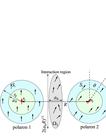
Figure 1: (Color online) Two electro-magnetic polarons in DMFE separated by a distance $R$. Red arrows show direction of electrons average magnetic moments. Angle between magnetic moments of two such electrons is $\theta$. The electrons wave function characteristic size is $\operatorname{\mathit{a}_{\mathrm{B}}}$. Black arrows show magnetic moments of impurities in DMFE. Within the magnetic polaron radius $r_{\mathrm{p}}$ they are co-directed with average impurity magnetic moment. In the central area between the polarons there is a lens shaped interaction region $\Omega_{\mathrm{i}}$. Impurities spins in this region are not fully polarized by donor electrons but correlated with them leading to interaction between the carriers. Width of the interaction region is about $\operatorname{\mathit{a}_{\mathrm{B}}}$. Lateral size of the region is about $2\sqrt{R\operatorname{\mathit{a}_{\mathrm{B}}}}$.

$$\hat{H}^{\mathrm{p-p}}_{\mathrm{e-imp}}=2Je^{-R/a_{\mathrm{B}}}(\hat{\mathbf{s}}_{1}+\hat{\mathbf{s}}_{2})\sum_{j\in\Omega_{\mathrm{i}}}\hat{\mathbf{S}}_{j}/S_{0},$$ (20)

where summation is over the region of interaction $\Omega_{\mathrm{i}}$. Number of impurities inside the interaction region can be estimated as $N_{\mathrm{i}}=\pi a_{\mathrm{B}}^{2}Rn_{\mathrm{i}}$. Treating the total polarons spins as classical magnetic moments we obtain

$$\hat{H}^{\mathrm{p-p}}_{\mathrm{e-imp}}=2Je^{-R/a_{\mathrm{B}}}\cos(\theta/2)\sum_{j\in\Omega_{\mathrm{i}}}\hat{\mathbf{S}}^{(z)}_{j}/S_{0},$$ (21)

where $\theta$ is the angle between average magnetic moments of polarons. We assume that both polarons are similar and have the same magnetic moment. $\hat{\mathbf{S}}^{(z)}_{j}$ is the projection of the impurity spin on the direction $\mathbf{m}_{1}+\mathbf{m}_{2}$. Interaction of donor electron and impurities in the region $\Omega_{\mathrm{i}}$ is weak. Therefore, the average magnetic moment created by this interaction is defined as $\langle\sum_{j\in\Omega_{\mathrm{i}}}\hat{\mathbf{S}}^{(z)}_{j}\rangle\approx 2N_{\mathrm{i}}S_{0}Je^{-R/a_{\mathrm{B}}}\cos(\theta/2)/(3k_{\mathrm{B}}T)$. Introducing this result into Eq. (21) we get the average interaction energy of two polarons

$$H^{\mathrm{p-p}}_{\mathrm{e-imp}}=\frac{4N_{\mathrm{i}}J^{2}e^{-2R/a_{\mathrm{B}}}\cos^{2}(\theta/2)}{3k_{\mathrm{B}}T}=H^{\mathrm{p-p}}(\cos(\theta)+1).$$ (22)

V Magnetic phase diagram of DMFE

The distance at which two polarons can be considered as coupled ($r_{\mathrm{c}}$) is defined by the condition

$$|H^{\mathrm{HL}}+H^{\mathrm{se}}+H^{\mathrm{p-p}}|=k_{\mathrm{B}}T.$$ (23)

Note that the Heitler-London coupling, $H^{\mathrm{HL}}>0$, and the superexchange, $H^{\mathrm{se}}>0$, produce antiferromagnetic (AFM) coupling while impurity mediated coupling is FM, $H^{\mathrm{p-p}}<0$. On one hand the first two interactions decay faster with distance ($e^{-2R/\operatorname{\mathit{a}_{\mathrm{B}}}}$) than the third one ($e^{-R/\operatorname{\mathit{a}_{\mathrm{B}}}}$). But on the other hand the impurity mediated interaction depends on concentration $n_{\mathrm{i}}$ and temperature. It decreases with increasing of temperature and reducing of $n_{\mathrm{i}}$. Experimental results on DMFE show that in most cases FM order appears at low magnetic impurities concentration [Xu et al., 2009; Lin et al., 2009; Kumari et al., 2017; Bai et al., 2009; Lee et al., 2003; Ye et al., 2011] meaning that impurity mediated coupling dominates. However, AFM order is also reported in DMFEs with low impurities concentration [Barbier et al., 2015].

In the case of $H^{\mathrm{HL}}_{0}=H^{\mathrm{se}}_{0}=0$, Eq. (23) for the interaction distance $r_{\mathrm{c}}$ at given temperature $T$ turns into

$$k_{\mathrm{B}}T=\frac{S_{0}J_{0}\sqrt{n_{\mathrm{i}}r_{\mathrm{c}}}e^{-r_{\mathrm{c}}/\operatorname{\mathit{a}_{\mathrm{B}}}}}{\sqrt{3\pi}a_{\mathrm{B}}^{2}}.$$ (24)

Approximately one can write

$$r_{\mathrm{c}}\sim\operatorname{\mathit{a}_{\mathrm{B}}}\left(\!\mathrm{ln}\!\left[\!\frac{S_{0}J_{0}}{2\pi\operatorname{\mathit{a}^{3}_{\mathrm{B}}}k_{\mathrm{B}}T}\right]\!+\frac{1}{2}\mathrm{ln}\left[\!\operatorname{\mathit{a}^{3}_{\mathrm{B}}}n_{\mathrm{i}}\mathrm{ln}\!\left(\frac{S_{0}J_{0}}{2\pi\operatorname{\mathit{a}^{3}_{\mathrm{B}}}k_{\mathrm{B}}T}\!\!\right)\!\!\right]\!\!\right).$$ (25)

According to percolation theory [Shklovskii and Efros, 1984] the long range magnetic order in the system of randomly situated polarons appears approximately at $r_{\mathrm{c}}n_{\mathrm{d}}^{1/3}=0.86$, where $n_{\mathrm{d}}$ is the defects concentration. Introducing $r_{\mathrm{c}}$ from this relation into Eq. (23) one can find the ordering temperature. Depending on the sign of the total interaction the ordering can be either FM or AFM (or superspin glass state).

First, consider the case when the polaron-polaron interaction is the dominant one and we can neglect the Heitler-London and superexchange contributions. In this case there is only FM type interaction between impurities and only the FM/paramagnetic (PM) transition is possible. The transition temperature is given by the equation

$$k_{\mathrm{B}}T=\frac{S_{0}J_{0}\sqrt{0.86n_{\mathrm{i}}}\exp{(-0.86/(\operatorname{\mathit{a}_{\mathrm{B}}}n_{\mathrm{d}}^{1/3}))}}{\sqrt{3\pi}n_{\mathrm{d}}^{1/6}a_{\mathrm{B}}^{2}}.$$ (26)

Note than according to Eqs. (5), (4) and (13) the Bohr radius, $\operatorname{\mathit{a}_{\mathrm{B}}}(T,E)$ depends on temperature and external electric field. This makes the PM/FM transition temperature more complicated function of $n_{\mathrm{i}}$ and $n_{\mathrm{d}}$ and makes it dependent on electric field.

Dimensionless magnetization of the DMFE is given by the following equation [Shklovskii and Efros, 1984; Kaminski and Sarma, 2002]

$$M(T)=S_{0}n_{\mathrm{i}}V_{\mathrm{inf}}((r_{\mathrm{c}}(T))^{3}n_{\mathrm{d}}),$$ (27)

where $V_{\mathrm{inf}}$ is the relative volume of infinite cluster (or probability that an impurity belongs to an infinite cluster) in site percolation problem. We found the function using Monte-Carlo simulations approach developed in Ref. [Holcomb and Jr., 1969].

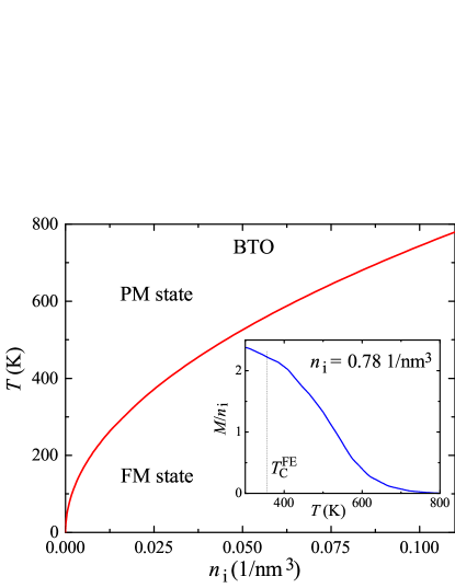
Figure 2: (Color online) Approximate magnetic phase transition temperature Eq. (26) as a function of impurities concentration $n_{\mathrm{i}}$. The system parameters, which correspond to BTO doped with Fe, are in the text. The inset is the magnetic moment per Fe impurity as a function of temperature for $n_{\mathrm{i}}=0.78$ 1/nm³ ($5$% doping).

V.1 BaTiO₃ based DMFE

Figure 2 shows the magnetic phase diagram of DMFE with the following parameters. Impurities magnetic moment is $S_{0}=5/2$. High frequency dielectric constant is $\operatorname{\varepsilon}_{\infty}=5.8$ and the static one is $\operatorname{\varepsilon}=1000$. We chose such a value of $m^{*}$ that $\operatorname{\mathit{a}_{\mathrm{B}}}=0.45$ nm. This corresponds to BTO crystal with Fe impurities. Concentration of defects (oxygen vacancies) is about 0.043 nm^-3 (0.27%, lattice period in BTO is about $0.4$ nm). Parameter $S_{0}J_{0}=6\cdot 10^{4}$ K$\cdot$nm³. At impurities concentration of about 5% this gives spin splitting of the carrier of about 2.4 eV. This splitting occurs due to interaction with all impurities within the polaron. We neglect the Heitler-London and superexchange contributions.

The figure shows magnetic state of the system as a function of impurities concentration and temperature. The system is FM at low temperatures and high impurities concentration and is PM at high temperatures and low concentration of magnetic impurities. The curve in Fig. 2 shows approximate boundary between these two magnetic states. For such a high dielectric constant the Bohr radius $\operatorname{\mathit{a}_{\mathrm{B}}}$ is independent of $\operatorname{\varepsilon}$ and the temperature dependence of the dielectric constant does not play any role in magnetic properties of the material.

The inset shows magnetization as a function of temperature for impurities concentration $n_{\mathrm{i}}=0.78$ 1/nm³ (5% for BTO crystal). Magnetic phase transition appears at $T\approx 650$ K. This is in agreement with experiment in Ref. [Xu et al., 2009]. Ferroelectric phase transition in BTO appears around $T^{\mathrm{FE}}_{\mathrm{C}}=$360 K. In this region the dielectric constant has a strong peak. However, because of very large $\operatorname{\varepsilon}$ the ME effect is weak and no peculiarities appear in the vicinity of $T^{\mathrm{FE}}_{\mathrm{C}}$.

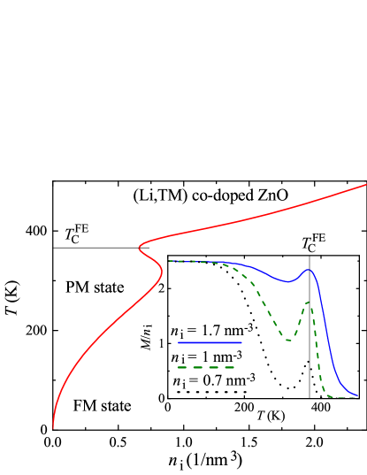
Figure 3: (Color online) Magnetic phase diagram of (Li,TM) co-doped ZnO. The system parameters are provided in the text. The inset is the magnetic moment per TM impurity as a function of temperature for $n_{\mathrm{i}}=1.7$ nm^-3 (solid blue line), $1$ nm^-3 (dashed green line) and $0.7$ nm^-3 (dotted black line).

V.2 ZnO based DMFE

(Li,TM) co-doped Zinc oxide is one of the most studied doped magnetic ferroelectrics [Zou et al., 2010, 2011; Lin et al., 2011]. Ordinarily, both ferroelectricity and magnetism in these materials appear due to doping. In contrast to “classical” FEs such as BTO, the ZnO based multiferroics have relatively low dielectric constant. Inevitable defects in doped ZnO materials also provides shallow donor states. Due to low dielectric constant of the material the Bohr radius of these states can be temperature dependent.

Magnetism in TM doped ZnO was theoretically and experimentally studied in numerous works [Pan et al., 2008; Venkatesan et al., 2004; Behan et al., 2008; Sluiter et al., 2005]. Two distinct cases were recognized when the material is either diluted magnetic semiconductor (DMS) or diluted magnetic insulator (DMI) [Behan et al., 2008]. In the first case carriers are delocalized on the scale of the whole sample and magnetic ordering appears due to Ruderman-Kittel-Kasuya-Yosida interaction. In the second case carriers are strongly localized and the coupling is due to magnetic polarons. We will assume the small concentration of defects and BMP based coupling.

Dielectric and magnetic properties in ZnO-based materials strongly depend on the dopand type, concentration and fabrication procedure. Figure 3 shows magnetic phase digram of the DMFE with parameters close to (TM,Li) co-doped ZnO. Impurities magnetic moment is $S_{0}=5/2$ and $S_{0}J_{0}=3.3\cdot 10^{4}$ K$\cdot$nm³ giving the spin splitting of the electron of about 1.7 eV for impurities concentration $n_{\mathrm{i}}=1$ nm^-3. High frequency dielectric constant is $\operatorname{\varepsilon}_{\infty}=4$ [Coey et al., 2005]. Static dielectric constant strongly depends on temperature with $\operatorname{\varepsilon}^{T}_{\mathrm{min}}=25$, $\Delta\operatorname{\varepsilon}^{T}=45$ and the ferroelectric Curie temperature, $T^{\mathrm{FE}}_{\mathrm{C}}=370$ K [Pan et al., 2009]. We chose $m^{*}$ such that $\operatorname{\mathit{a}_{\mathrm{B}}}=0.75$ nm at zero temperature [Coey et al., 2005]. Concentration of defects (oxygen vacancies) is about 0.02 nm^-3 ($\sim$0.1%). We neglect Heitler-London and superexchange contributions.

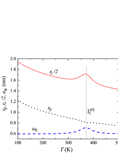
Figure 4: (Color online) The Bohr radius $\operatorname{\mathit{a}_{\mathrm{B}}}$, BMP radius $r_{\mathrm{p}}$ and BMP interaction distance $r_{\mathrm{c}}$ as a function of temperature for DMFE with $\operatorname{\varepsilon}$ described by Eq. (4) with $\operatorname{\varepsilon}_{\mathrm{min}}=25$, $\Delta\operatorname{\varepsilon}=45$, $T^{\mathrm{FE}}_{\mathrm{C}}=370$ K and $\operatorname{\varepsilon}_{\infty}=4$. Effective mass is chosen such that the Bohr radius at zero temperature is $\operatorname{\mathit{a}_{\mathrm{B}}}=0.75$ nm.

Magnetic phase transition curve has a peculiarity in the vicinity of FE phase transition temperature $T^{\mathrm{FE}}_{\mathrm{C}}=370$ K. The peculiarity is related to non-monotonic behavior of the BMP coupling radius $r_{\mathrm{c}}$ in the vicinity of $T^{\mathrm{FE}}_{\mathrm{C}}$ (see Fig. 4). Since static dielectric constant is comparable to optical one and it has a peak as a function of temperature at $T=T^{\mathrm{FE}}_{\mathrm{C}}$ the Bohr radius also has a peak in this region. Increasing $\operatorname{\mathit{a}_{\mathrm{B}}}$ leads to the increase of BMP interaction distance $r_{\mathrm{c}}$ and enhancement of magnetic properties. Note that while the Bohr radius $\operatorname{\mathit{a}_{\mathrm{B}}}$ and interaction distance $r_{\mathrm{c}}$ have a peak in the vicinity of FE phase transition, the BMP radius $r_{\mathrm{p}}$ has a deep (at least for given parameters).

Inset in Fig. 3 shows magnetization of DMFE as a function of temperature for several concentrations of TM impurities. Magnetization also has a peak at $T=T^{\mathrm{FE}}_{\mathrm{C}}$. Such a peak is the consequence of coupling between electric and magnetic subsystems in this material and can be considered as magneto-electric effect.

In Refs. [Zou et al., 2011; Pan et al., 2009] temperature dependence of (Li,TM) co-doped ZnO magnetization were studied in the vicinity of FE phase transition. No peculiarities in magnetization in the vicinity of the FE transition point were observed. Two possible reasons for the absence of magneto-electric coupling in these particular samples may exist. The first one is that samples studied in Ref. [Zou et al., 2011] are nanorods of (Li,Co) co-doped ZnO with very large surface/volume ratio. The origin of magnetism in such structures is also under question. On one hand the conductivity of these samples is small meaning that the material is DMI with possible BMP-based magnetism. On the other hand the magnetism can be related to surface effects as often happens in nanoscale metal oxides [Escudero and Escamilla, 2011; Sundaresan and Rao, 2009]. The second possible reason is that the model of electric polaron described in Sec. III.2 is not applicable to this particular material. Ferroelectricity in this material is related to Li doping and oxygen vacancies [Zou et al., 2011]. Electric dipoles in this material are inhomogeneously spread across the sample. Therefore, the low-frequency dielectric constant related to these dipoles should be also rather inhomogeneous. Inhomogeneity of dielectric constant probably appears at the same spatial scale as the distance between magnetic polarons in the system. Therefore, electric dipoles responsible for ferroelectricity and static dielectric constant do not influence the polaron size.

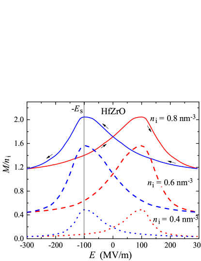
Figure 5: (Color online) Dimensionless magnetic moment per magnetic impurity (maximum moment is $S_{0}=5/2$) as a function of applied electric field $E$ for $n_{\mathrm{i}}=0.8$ nm^-3 (solid lines), $0.6$ nm^-3 (dashed lines) and $0.4$ nm^-3 (dotted lines). Arrows show the hysteresis bypass direction.

V.3 Hf_xZr_1-xO₂ based DMFE

Another FEs family with low dielectric constant is materials based on HfO₂. Doping of Hf oxide with various elements leads to the appearance of FE properties (spontaneous electric polarization, hysteresis loop, electric field dependent dielectric constant) [Boscke et al., 2011; Muller et al., 2011, 2012]. In the present work we discuss Hf_0.5Zr_0.5O₂ FE [Muller et al., 2012]. This material is homogeneous in contrast to FEs based on weakly doped zinc oxide. This allows to expect that variation of dielectric constant in this material leads to variation of polaron size. The source of carriers in this material is also oxygen vacancies. No data is available on magnetic doping of this material.

Dielectric constant of Hf_0.5Zr_0.5O₂ depends on external electric field. Therefore, one can control magnetic properties of Hf_0.5Zr_0.5O₂ doped with magnetic impurities using electric field. Figure 5 shows the dependence of magnetization of DMFE on external electric field at room temperature and for different impurity concentrations. Other parameters are chosen as follows. The Bohr radius at zero electric field is 0.5 nm. Impurities magnetic moment is $S_{0}=5/2$ and $S_{0}J_{0}=3.3\cdot 10^{4}$ K$\cdot$nm³ giving the spin splitting of the electron of about 1.1 eV for impurities concentration $n_{\mathrm{i}}=1$ nm^-3. Defects concentration is $n_{\mathrm{d}}=0.05$ nm^-3 ($\sim 0.6$% in the case of Hf_0.5Zr_0.5O₂ which has the lattice constant of 0.5 nm). Optical dielectric constant $\operatorname{\varepsilon}_{\infty}=4.5$. Static dielectric constant as a function of electric field is given by Eq. (4) with $\operatorname{\varepsilon}^{E}_{\mathrm{min}}=30$, $\Delta\operatorname{\varepsilon}^{E}=15$, $E_{\mathrm{s}}=100$ MV/m and switching region width $\Delta E_{\mathrm{s}}=E_{\mathrm{s}}$ [Muller et al., 2012]. The Heitler-London and superexchange contributions are neglected.

Static dielectric constant depends on electric field leading to electric field dependence of magnetization in the system (ME effect). $\operatorname{\varepsilon}$ demonstrates hysteresis behavior causing hysteresis of magnetization as a function of electric field $E$. Dielectric constant reaches its maximum at the switching field $\pm E_{\mathrm{s}}$. According to Eq. (25) the BMP interaction distance grows with $\operatorname{\varepsilon}$. Therefore, the magnetization has peaks at $E=\pm E_{\mathrm{s}}$. While interaction distance variation is not large (about 10%) the magnetization variation is significant.

V.4 Influence of Heitler-London and superexchange contributions

Since the Heitler-Lodon and superexchange interactions are antiferromagnetic ones, they compete with the BMP-based coupling. These interactions decay faster with distance between defects than the impurities mediated magnetic coupling, but they do not depend on concentration $n_{\mathrm{i}}$ and temperature. Therefore, at low impurities concentration and high temperature antiferromagnetic interactions can dominate leading to antiferromagnetic (or spin glass) ordering. At temperature independent dielectric constant the AFM ordering temperature can be found as follows

$$T^{\mathrm{AFM}}=\frac{H^{\mathrm{HL}}+H^{\mathrm{se}}\pm\sqrt{(H^{\mathrm{HL}}+H^{\mathrm{se}})^{2}+4\tilde{H}^{\mathrm{p-p}}}}{2},$$ (28)

where $\tilde{H}^{\mathrm{p-p}}=-H^{\mathrm{p-p}}k_{\mathrm{B}}T$. Solutions exist only if $H^{\mathrm{HL}}+H^{\mathrm{se}}>2\sqrt{H^{\mathrm{p-p}}k_{\mathrm{B}}T}$. This condition is alway satisfied at low enough impurities concentration. Competition between AFM and FM interactions in DMS was considered in Ref. [Durst et al., 2002].

Figure 6 shows magnetic phase diagram of DMFE with significant contribution of the Heitler-London and superexchange interactions. The following parameters are used. $S_{0}=5/2$, $S_{0}J_{0}=4\cdot 10^{4}$ K/nm³, $n_{\mathrm{d}}=0.02$ nm^-3, $m^{*}$ is chosen such that the Bohr radius away from $T^{\mathrm{FE}}_{\mathrm{C}}$ is about $0.75$ nm, $\operatorname{\varepsilon}_{\mathrm{\infty}}=4$, $\operatorname{\varepsilon}_{\mathrm{min}}^{T}=25$, $\Delta\operatorname{\varepsilon}^{T}=35$, $\Delta T=20$ K, $T^{\mathrm{FE}}_{\mathrm{C}}=370$ K, $H^{\mathrm{HL}}_{0}=3.5\cdot 10^{7}$ K (main graph), $H^{\mathrm{se}}_{0}=5\cdot 10^{3}$ K/nm (red curves), $10\cdot 10^{3}$ K/nm (green curves), $15\cdot 10^{3}$ K/nm (blue curves). In the inset we use $H^{\mathrm{HL}}_{0}=5\cdot 10^{6}$ K, $H^{\mathrm{se}}_{0}=3\cdot 10^{3}$ K/nm.

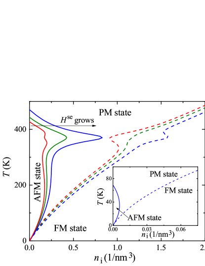
Figure 6: (Color online) Magnetic phase diagram of DMFE with strong Heitler-London and superexchange interactions. Solid lines show boundary between PM and AFM states, dashed lines demonstrate PM/FM transition. All curves are plotted for the same $H^{\mathrm{HL}}_{0}$. Red lines correspond to the system with the smallest superexchange contribution, green lines show magnetic phase diagram for a system with intermediate $H^{\mathrm{se}}_{0}$ and blue curves are for the highest $H^{\mathrm{se}}_{0}$. All system parameters are provided in the text. Main figure shows the situation of strong direct coupling leading to AFM ordering in the vicinity of FE phase transition. Inset shows the case when direct coupling ($H^{\mathrm{HL}}$ and $H^{\mathrm{se}}$) is weak and induce AFM states only at low temperature.

In contrast to the previously considered cases the region of AFM ordering appears at finite $H^{\mathrm{HL}}$ and/or $H^{\mathrm{se}}$. FM/PM boundary also changes. Region of AFM ordering exist only at low impurity concentration, since only in this case AFM interactions overcome strong impurity mediated FM coupling. The main figure shows the case where direct interactions ($H^{\mathrm{HL}}$ and $H^{\mathrm{se}}$) are strong and induce AFM ordering at high temperatures close to FE phase transition. Note that Heitler-London interaction decreases with increasing of dielectric constant while the superexchange interaction behaves oppositely. Therefore, behavior of the phase boundaries strongly depends on the ratio between these two contributions. Superexchange mostly influences the region in the vicinity of FE phase transition. AFM region grows and FM region decreases with increasing of $H^{\mathrm{se}}_{0}$ in the vicinity of $T^{\mathrm{FE}}_{\mathrm{C}}$. Heitler-London interaction influences the phase diagram aside of $T^{\mathrm{FE}}_{\mathrm{C}}$, but this influence is mostly quantitative.

Inset shows the case when $H^{\mathrm{HL}}$ and/or $H^{\mathrm{se}}$ are relatively small and do not lead to magnetic ordering in the vicinity of FE phase transition. In this case modifications of FM/PM boundary is weak. AFM region exists at low temperatures and low impurities concentration.

VI Conclusion

In the present work we proposed a coupling mechanism of magnetic and electric degrees of freedom in doped magnetic ferroelectrics. Magnetic order in DMFE appears due to formation and interaction of BMPs. There are three different contributions into interaction between magnetic polarons. All these contributions depend on dielectric constant of the FE matrix. The most significant is the impurities mediated interaction between polarons. It depends on the radius of polaron wave function. Due to interaction with phonons this radius linearly depends on the dielectric constant of FE matrix. Since the dielectric constant of FEs can be controlled with applied field or varying temperature, one can control the interpolaron interaction and magnetic state of the whole system. Peculiarity of this magneto-electric effect is that it does not involve the relativistic spin-orbit coupling and relies only on the Coulomb interaction.

We calculated magnetic phase transition temperatures as a function of impurities concentration and showed that strong temperature dependence of dielectric permittivity in the vicinity of FE phase transition leads to essential modification of magnetic phase diagram. We found magnetization as a function of temperature and showed that it has a peak in the vicinity of FE phase transition. This peak is a consequence of ME effect appearing in DMFE.

We calculated magnetization as a function of electric field in DMFE and demonstrated that magnetic moment of the system can be effectively controlled with applied bias. Magnetization shows hysteresis behavior as a function of electric field. It has two peaks associated with FE polarization switching.

Strong magneto-electric coupling can appear only in DMFE with low dielectric constant such as (Li,TM) co-doped ZnO or Hf_0.5Zr_0.5O₂. TM-doped BaTiO₃ is not a very promising candidate to observe our effect due to very larger dielectric constant.

VII Acknowledgements

This research was supported by NSF under Cooperative Agreement Award EEC-1160504 and NSF PREM Award. O.U. was supported by Russian Science Foundation (Grant 16-12-10340).

References

- Lilienblum et al. (2015) M. Lilienblum, T. Lottermoser, S. Manz, S. M. Selbach, A. Cano, and M. Fiebig, Nature Physics 11, 1070 (2015).
- Eerenstein et al. (2006) W. Eerenstein, N. D. Mathur, and J. F. Scott, Nature 442, 759 (2006).
- Ramesh and Spaldin (2007) R. Ramesh and N. A. Spaldin, Nature Mat. 6, 21 (2007).
- Zheng et al. (2004) H. Zheng, J. Wang, S. E. Lofland, Z. Ma, L. Mohaddes-Ardabili, T. Zhao, L. Salamanca-Riba, S. R. Shinde, S. B. Ogale, F. Bai, D. Viehland, Y. Jia, D. G. Schlom, M. Wuttig, A. Roytburd, and R. Ramesh, Science 303, 661 (2004).
- Bibes and Barthelemy (2008) M. Bibes and A. Barthelemy, Nature Mat. 7, 425 (2008).
- Mathur (2008) N. Mathur, Nature 454, 591 (2008).
- Barbier et al. (2015) A. Barbier, T. Aghavnian, V. Badjeck, C. Mocuta, D. Stanescu, H. Magnan, C. L. Rountree, R. Belkhou, P. Ohresser, and N. Jedrecy, Phys. Rev. B 91, 035417 (2015).
- Luo et al. (2009) L. B. Luo, Y. G. Zhao, H. F. Tian, J. J. Yang, J. Q. Li, J. J. Ding, B. He, S. Q. Wei, and C. Gao, Phys. Rev. B 79, 115210 (2009).
- Xu et al. (2009) B. Xu, K. B. Yin, J. Lin, Y. D. Xia, X. G. Wan, J. Yin, X. J. Bai, J. Du, and Z. G. Liu, Phys. Rev. B 79, 134109 (2009).
- Maier and Cohn (2002) R. Maier and J. L. Cohn, J. Appl. Phys. 92, 5429 (2002).
- Lin et al. (2009) Y.-H. Lin, J. Yuan, S. Zhang, Y. Zhang, J. Liu, Y. Wang, and C.-W. Nan, Appl. Phys. Lett. 95, 033105 (2009).
- Shuai et al. (2011) Y. Shuai, S. Zhou, D. Burger, H. Reuther, I. Skorupa, V. John, M. Helm, and H. Schmidt, J. Appl. Phys. 109, 084105 (2011).
- Bai et al. (2009) W. Bai, X. J. Meng, T. Lin, L. Tian, C. B. Jing, W. J. Liu, J. H. Ma, J. L. Sun, and J. H. Chu, J. Appl. Phys. 106, 124908 (2009).
- Wei et al. (2011) X. K. Wei, Y. T. Su, Y. Sui, Q. H. Zhang, Y. Yao, C. Q. Jin, and R. C. Yu, J. Appl. Phys. 110, 114112 (2011).
- Wang et al. (2009) Y. Wang, G. Xu, X. Ji, Z. Ren, W. Weng, P. Du, G. Shen, and G. Han, Journal of Alloys and Compounds 475, L25 (2009).
- Kumari et al. (2017) M. Kumari, D. G. B. Diestra, R. Katiyar, J. Shah, R. K. Kotnala, and R. Chatterjee, J. Appl. Phys. 121, 034101 (2017).
- Ye et al. (2011) X. Ye, Z. Zhou, W. Zhong, D. Hou, H. Cao, C. Au, and Y. Du, Thin Solid Films 519, 2163 (2011).
- Shah and Kotnala (2013) J. Shah and R. K. Kotnala, J. Mater. Chem. A 1, 8601 (2013).
- Coey et al. (2005) J. M. D. Coey, M. Venkatesan, and C. B. Fitzgerald, Nature Mat. 4, 173 (2005).
- Dietl and Spalek (1983) T. Dietl and J. Spalek, Phys. Rev. B 28, 1548 (1983).
- Angelescu and Bhatt (2001) D. E. Angelescu and R. N. Bhatt, Phys. Rev. B 65, 075211 (2001).
- Durst et al. (2002) A. C. Durst, R. N. Bhatt, and P. A. Wolff, Phys. Rev. B 65, 235205 (2002).
- Kaminski and Sarma (2002) A. Kaminski and S. D. Sarma, Phys. Rev. Lett. 88, 247202 (2002).
- Udalov et al. (2015a) O. G. Udalov, N. M. Chtchelkatchev, and I. S. Beloborodov, J. Phys.: Condens. Matter 27, 186001 (2015a).
- Udalov et al. (2015b) O. G. Udalov, N. M. Chtchelkatchev, and I. S. Beloborodov, Phys. Rev. B 92, 045406 (2015b).
- Udalov and Beloborodov (2017a) O. G. Udalov and I. S. Beloborodov, Phys. Rev. B 95, 045427 (2017a).
- Udalov and Beloborodov (2017b) O. G. Udalov and I. S. Beloborodov, J. Phys.: Condens. Matter 29, 175804 (2017b).
- Udalov and Beloborodov (2017c) O. G. Udalov and I. S. Beloborodov, J. Phys.: Condens. Matter 29, 155801 (2017c).
- Mitra et al. (1987) T. K. Mitra, A. Chati’erjee, and S. Mukhopadhyay, Physics Rep. 153, 91 (1987).
- Whitfield and Platzman (1972) G. Whitfield and P. M. Platzman, Phys. Rev. B 6, 3987 (1972).
- Hattori (1975) K. Hattori, Journal of the Physical Society of Japan 38, 669 (1975).
- Engineer and Whitfield (1969) M. Engineer and G. Whitfield, Phys. Rev. 179, 869 (1969).
- Boscke et al. (2011) T. S. Boscke, S. Teichert, D. Brauhaus, J. Muller, U. Schroder, U. Bottger, and T. Mikolajick, Appl. Phys. Lett. 99, 112904 (2011).
- Muller et al. (2011) J. Muller, U. Schroder, T. S. Boscke, I. Muller, U. Bottger, L. Wilde, J. Sundqvist, M. Lemberger, P. Kucher, T. Mikolajick, and L. Frey, J. Appl. Phys. 110, 114113 (2011).
- Muller et al. (2012) J. Muller, T. S. Boscke, U. Schroder, S. Mueller, D. Brauhaus, U. Bottger, L. Frey, and T. Mikolajick, Nano Lett. 12, 4318 (2012).
- Pan et al. (2008) F. Pan, C. Song, X. J. Liu, Y. C. Yang, and F. Zeng, Materials Science and Engineering R 62, 1 (2008).
- Venkatesan et al. (2004) M. Venkatesan, C. B. Fitzgerald, J. G. Lunney, and J. M. D. Coey, Phys. Rev. Lett. 93, 177206 (2004).
- Behan et al. (2008) A. J. Behan, A. Mokhtari, H. J. Blythe, D. Score, X.-H. Xu, J. R. Neal, A. M. Fox, and G. A. Gehring, Phys. Rev. Lett. 100, 047206 (2008).
- Sluiter et al. (2005) M. H. F. Sluiter, Y. Kawazoe, P. Sharma, A. Inoue, A. R. Raju, C. Rout, and U. V. Waghmare, Phys. Rev. Lett. 94, 187204 (2005).
- Wolff (1988) P. A. Wolff, Semiconductors and Semimetals 25, 413 (1988).
- Larsen (1969) D. M. Larsen, Phys. Rev. 187, 1147 (1969).
- Zou et al. (2009) C. W. Zou, M. Li, H. J. Wanga, M. L. Yin, C. S. Liu, L. P. Guo, D. J. Fu, and T. W. Kang, Nuclear Instruments and Methods in Physics Research B 267, 1067 (2009).
- Dhananjay et al. (2006) Dhananjay, J. Nagaraju, and S. B. Krupanidhi, Journal of Applied Physics 99, 034105 (2006).
- Gupta and Kumar (2011) M. K. Gupta and B. Kumar, Journal of Alloys and Compounds 509, L208 (2011).
- Awan’ et al. (2014) S. U. Awan’, S. K. Hasanain’, G. H. Jaffari, and Z. Mehmood, Appl. Phys. Lett. 104, 222906 (2014).
- Auerbach (1994) A. Auerbach, Interacting Electrons and Quantum Magnetism (Spiringe-Verlag New York, 1994).
- Lee et al. (2003) J. Lee, Z. Khim, Y. Park, D. Norton, N. Theodoropoulou, A. Hebard, J. Budai, L. Boatner, S. Pearton, and R. Wilson, Solid-State Electronics 47, 2225 (2003).
- Shklovskii and Efros (1984) B. I. Shklovskii and A. L. Efros, Electronic Properties of Doped Semiconductors (Spiringe-Verlag Berlin, 1984).
- Holcomb and Jr. (1969) D. F. Holcomb and J. J. R. Jr., Phys. Rev. 183, 773 (1969).
- Zou et al. (2010) C. W. Zou, H. J. Wanga, M. L. Yin, M. Li, C. S. Liu, L. P. Guo, D. J. Fu, and T. Kang, Journal of Crystal Growth 312, 906 (2010).
- Zou et al. (2011) C. W. Zou, L. X. Shao, L. P. Guo, D. J. Fu, and T. W. Kang, Journal of Crystal Growth 331, 44 (2011).
- Lin et al. (2011) Y.-H. Lin, M. Ying, M. Li, X. Wang, and C.-W. Nan, Appl. Phys. Lett. 90, 222110 (2011).
- Pan et al. (2009) F. Pan, X. jing Liu, Y. chao Yang, C. Song, and F. Zeng, Materials Science Forum 620, 1735 (2009).
- Escudero and Escamilla (2011) R. Escudero and R. Escamilla, Solid State Commun. 151, 97 (2011).
- Sundaresan and Rao (2009) A. Sundaresan and C. N. R. Rao, Nano Today 4, 96 (2009).