Impact of Neutrino Opacities on Core-Collapse Supernova Simulations

Abstract

Accurate description of neutrino opacities is central both to the core-collapse supernova (CCSN) phenomenon and to the validity of the explosion mechanism itself. In this work, we study in a systematic fashion the role of a variety of well-selected neutrino opacities in CCSN simulations where multi-energy, three-flavor neutrino transport is solved by the isotropic diffusion source approximation (IDSA) scheme. To verify our code, we first present results from one-dimensional (1D) simulations following core-collapse, bounce, and up to $\sim 250$ ms postbounce of a $15M_{\odot}$ star using a standard set of neutrino opacities by Bruenn (1985). Detailed comparison with published results supports the reliability of our three-flavor IDSA scheme using the standard opacity set. We then investigate in 1D simulations how the individual opacity update leads to the difference from the base-line run with the standard opacity set. By making a detailed comparison with previous work, we check the validity of our implementation of each update in a step-by-step manner. Individual neutrino opacities with the largest impact on the overall evolution in 1D simulations are selected for a systematic comparison in our two-dimensional (2D) simulations. Special emphasis is devoted to the criterion of explodability in the 2D models. We discuss the implications of these results as well as the limitations and requirements for future towards more elaborate CCSN modeling.

1 Introduction

A core-collapse supernova (CCSN) is triggered when the core of a massive star becomes gravitational unstable, predominantly due to electron captures on protons bound in heavy iron-group nuclei. The collapse proceeds supersonically until the central density exceeds nuclear saturation density, when the repulsive nuclear force balances gravity such that the core bounces back with the formation of a hydrodynamics shock wave. This bounce shock propagates quickly to radii on the order of 100 km. However, the shock eventually turns into an accretion front due to losses from neutrinos, when propagating across the neutrinosphere of last scattering, as well as the continuous dissociation of infalling heavy nuclei from the still gravitationally unstable layers above the stellar core. The revival of this standing accretion shock is subject to the so-called supernova problem, i.e. the liberation of energy available at the interior of the proto-neutron star (PNS), the central hot and compact object, into a thick layer of accumulated material behind the shock front (for details, see Janka et al. (2007) for review).

Neutrinos play crucial roles during all phases of CCSNe - stellar core collapse, core bounce, postbounce mass accretion, onset of the explosion and PNS deleptonization, until cooling of neutron stars (NSs) (e.g., Woosley et al. (2002); Langanke & Martínez-Pinedo (2003); Janka (2017b); Yakovlev & Pethick (2004) for detailed reviews). In particular, during the stellar core collapse nuclear electron-capture rates determine the deleptonization (cf. Hix et al., 2003; Langanke et al., 2003), which in turn defines the location of the bounce shock. After bounce, the huge gravitational energy stored in the proto-neutron star (PNS) is almost completely carried away by neutrinos. A tiny fraction of the streaming neutrinos deposits energy in the postshock material via weak interactions, leading to an explosion in the neutrino-driven mechanism of CCSNe (Colgate & White, 1966; Wilson, 1985; Bethe & Wilson, 1985).

Multi-dimensional (multi-D) hydrodynamic instabilities play a crucial role in the neutrino mechanism. Non-linear turbulent flows associated with convective overturn and the standing-accretion-shock-instability (SASI, Blondin et al. (2003)) increase the neutrino heating efficiency in the gain region, essentially aiding the explosion (see Janka (2017a); Müller (2016); Hix et al. (2016); Foglizzo et al. (2015); Burrows (2013); Kotake et al. (2012) for reviews). In fact, a growing number of neutrino-driven models have been reported so far in self-consistent two-dimensional (2D) simulations, which has supported the validity of the multi-D neutrino-driven mechanism (e.g., Marek & Janka (2009); Suwa et al. (2010); Müller et al. (2012a); Dolence et al. (2014); Nakamura et al. (2015); Pan et al. (2016); O’Connor & Couch (2015); Burrows et al. (2016); Summa et al. (2016); Nagakura et al. (2017); Müller et al. (2017)).

This success is, however, highlighting new questions. The most challenging self-consistent three-dimensional (3D) simulations with spectral neutrino transport have failed to produce explosions for $11.2$, $20.0$, and $27.0M_{\odot}$ progenitors (Hanke et al. (2013); Tamborra et al. (2014), see, however, Roberts et al. (2016) for an exploding 27 $M_{\odot}$ model). In a few successful cases, the explosions are more delayed in 3D than in 2D (e.g., Lentz et al. (2015) and Melson et al. (2015a)), leading to smaller explosion energies in 3D compared to 2D (Takiwaki et al. (2014)). A few exceptions from this trend have been reported for 9.6 and 11.2 $M_{\odot}$ stars (Melson et al., 2015b; Müller, 2015). However, these two progenitors close to the low-mass end of the SN progenitors, may be rather peculiar in the sense that the 9.6 $M_{\odot}$ star has a tenuous envelope and explodes even in the one-dimensional (1D) simulation, that the 11.2 $M_{\sun}$ star is seemingly very marginal to produce 3D explosion (Müller, 2015; Takiwaki et al., 2012, 2014) or not (Hanke et al., 2013) with its progenitor’s compactness parameter being smallest among 101 solar-metallicity progenitors in Woosley et al. (2002).

One of the prime candidates to enhance the ”explodability” is to update neutrino physics in the multi-D models. Horowitz (2002) pioneeringly pointed out that the contribution of strange quarks to neutrino-nucleon scattering can affect neutrino opacity by $\sim 10-20\%$ (see also Kolbe et al. (1998)). In fact, Melson et al. (2015a) obtained 3D explosions of a $20M_{\odot}$ star only when the strageness effect was taken into account. Burrows et al. (2016) reported in their 2D self-consistent simulations of a 20 $M_{\odot}$ star that many-body corrections to neutrino-nucleon scattering (e.g., Horowitz et al. (2017); Burrows & Sawyer (1999, 1998) albeit in the different context) make explosions easier, increase explosion energy, and shorten the time to explosion.

Other intriguing possibilities to impact the CCSN explodability include general relativity (GR, e.g., Müller et al. (2012a); Kuroda et al. (2012, 2016); Roberts et al. (2016)), stellar rotation (e.g., Yamasaki & Foglizzo (2008); Marek & Janka (2009); Suwa et al. (2010); Nakamura et al. (2014a); Takiwaki et al. (2016); Summa et al. (2018); Kazeroni et al. (2017)), magnetic fields (e.g., Kotake et al. (2006); Endeve et al. (2012); Guilet & Müller (2015); Masada et al. (2015); Obergaulinger & Aloy (2017)), and inhomogeneities in the progenitor’s burning shells (e.g., Couch & Ott (2013); Couch et al. (2015); Müller (2015); Abdikamalov et al. (2016); Müller et al. (2017)).

Joining in the effort to update neutrino physics in CCSN codes, we investigate in this study impact of neutrino opacities in 1D and 2D core-collapse simulations where three-species neutrino transport is solved by the isotropic diffusion source approximation scheme (IDSA, Liebendörfer et al. (2009)). We first start with 1D simulations where we use the same input physics and the same equation of state (EOS) as those in Liebendörfer et al. (2005). In the seminal work, detailed comparison between the two reference codes between Agile-BOLTZTRAN (Liebendörfer et al., 2004; Mezzacappa & Bruenn, 1993a) and VERTEX(-PROMETHEUS) (Rampp & Janka, 2002a) was made. Their results are available online, so that we are able to make a comparison with their data set. In the original IDSA scheme (Liebendörfer et al., 2009), a base-line set of neutrino opacities (Bruenn, 1985) (often referred to as the Bruenn rate) is used. Following the implementation schemes of microphysical update in the literature (e.g., Buras et al. (2006b); Fischer et al. (2009); Fischer (2016)), we study how individual update in the neutrino opacity leads to differences from the base-line run with the Bruenn rate. From these systematic 1D runs, we could have a guess which update could potentially help (or harm) the explodability in multi-D models. Then we move on to perform 2D simulations where several sets of neutrino opacities are included. This is because a full investigatation of the individual rates is currently too computationally expensive to do in multi-D simulations.

This paper is organized as follows. In Section 2, we summarize numerical methods including model setup, neutrino opacities, and the three-flavor IDSA scheme. In Section 3, we first compare our results with Liebendörfer et al. (2005) (Section 3.1). Then we proceed to study impact of the individual (updated) rates in 1D runs one by one from Section 3.2 to 3.6. Then it may be interesting to see which expectations regarding the explodability of the 1D models survive when we perform 2D simulations (Section 4). We summarize our results and discuss its implications in Section 5.

2 Numerical methods

2.1 Model setup

In our 1D simulations, we employ a standard 15$M_{\odot}$ progenitor (“s15s7b2” in Woosley & Weaver, 1995), following the work by Liebendörfer et al. (2005). To see effects of individual neutrino rates, we follow the dynamics starting from core collapse, through bounce, up to $\sim 500$ ms postbounce (pb) in each 1D run. In our 2D runs, we choose a 20$M_{\odot}$ progenitor model of Woosley & Heger (2007) that has been widely used in recent multi-D simulations (e.g., Melson et al. (2015a); Burrows et al. (2016); Bollig et al. (2017)). This progenitor is characterized by high explodability where the neutrino-driven shock revival was obtained around $\sim 250$ ms (pb) at the earlist in the literature (e.g., Melson et al. (2015a); Summa et al. (2016); O’Connor & Couch (2015)).

Our non-relativistic hydrodynamics code employs a high-resolution shock capturing scheme with an approximate Riemann solver of Einfeldt (1988) (see Nakamura et al. (2015) for more details). Self-gravity is computed by a monopole approximation with an approximate treatment of GR gravity by the effective potential of Case A of Marek et al. (2006). Our 1D and 2D runs are computed on a spherical polar grid with a resolution of $n_{r}=512$, and $n_{r}\times n_{\theta}$ = $512\times 128$, respectively. Non-equally spacial radial zones covers from the center to an outer boundary of $5\times 10^{8}$ cm. The radial grid is chosen such that the resolution $\Delta r$ is better than 250m in the PNS interior and typically better than 1km outside the PNS. Seed perturbations for aspherical instabilities are imposed by hand at 10 ms after bounce by introducing random perturbations of $1\%$ in velocity behind the stalled shock. For the spectral transport, we use 20 logarithmically spaced energy bins ranging from 3 to 300 MeV. In our multi-D runs, we take into account the energy feedback from nuclear burning processes into hydrodynamic evolution by solving a 13-species $\alpha$-nuclei network (see Nakamura et al. (2014b) for details).

Throughout the paper, we use the EOS of Lattimer & Swesty (1991) (LS). Only in Section 3.1, we set the incompressibility parameter of $K=180$ MeV (LS180) for the sake of comparison with Liebendörfer et al. (2005), whereas in all the other models, we set $K=220$ MeV (LS220) that can account for the 2 $M_{\odot}$ NS mass measurements (Demorest et al., 2010; Antoniadis et al., 2013).

2.2 Neutrino opacities

Regarding neutrino opacities, our base-line model (set1, see Table 1) employs the standard weak interaction set given in Bruenn (1985) plus nucleon-nucleon bremsstrahlung (Hannestad & Raffelt, 1998) (see also Rampp & Janka (2002b) for detailed implementation schemes). Note in set1, ion-ion correlations for neutrino scattering on heavy nuclei (Horowitz, 1997) and the correction form factor (Mezzacappa & Bruenn, 1993a; Rampp & Janka, 2002b) are also included. In 1D runs, all the following update is basically added individually to the set1.

In set2 (see Table 1), electron capture (EC) rate on nuclei in set1 (Fuller et al., 1982) is replaced with the currently most elaborate one by Juodagalvis et al. (2010) which is a significant extension of the EC rate by Langanke et al. (2003) (see Section 2). In set3, electron neutrino pair annhilation into $\mu/\tau$ neutrinos (set3a in Table 1) and $\mu/\tau$-neutrino scattering on electron (anti)neutrinos (set3b) (Buras et al., 2003) is added to set1, respectively (see Appendices A and B for details). In set4a, medium modification to electron(/positron) capture reactions on proton(/neutron) are taken into account (Martínez-Pinedo et al., 2012; Roberts et al., 2012; Hempel, 2015; Roberts & Reddy, 2017) at the mean-field level (Reddy et al., 1998) (see Section 3.4). Set4b includes medium dependent suppresion of Bremsstrahlung (Fischer (2016), their Equation (11)).

In set5a, inelastic contributions and weak magnetism corrections are included following Horowitz (2002) for the charged current absorption and neutral current scattering processes. Set5b includes correction to the effective nucleon mass (Reddy et al., 1999). Following Buras et al. (2006b) (their Equation (A.1)), we replace the nucleon mass ($m_{N}$) with the density-dependent nucleon mass ($m^{*}_{N}(\rho)$), which accordingly changes the neutrino opacities.

In set6a, quenching of the axial-vector coupling constant at high densities (Carter & Prakash, 2002) (e.g., Equation (A.9) in Buras et al. (2006b)) is included but using more recent fitting formula (e.g., Equation (8) in Fischer (2016)). In set6b, we employ the formulas suggested by Horowitz et al. (2017) for the neutral-current axial response that accounts for virial effects at low density and many-body correlations at high densities (their Equations (36-39)). Finally in set6c, a strangeness-dependent contribution to the axial-vector coupling constant (Horowitz, 2002) with $g^{s}_{A}=-0.1$ (Hobbs et al., 2016) is considered for neutrino-nucleon scattering.

Note that even the full set in Table 1 is no way complete. Inclusion of muons significantly effects explodability (Bollig et al., 2017) and a proper treatment of nucleon kinematics (Reddy et al., 1998) is not taken in account in our full set (roles of nuclear de-excitation (Fischer et al., 2013) and light nuclear clusters (Sumiyoshi & Röpke, 2008) are also not included yet). These updates are another major undertaking, which we leave for future work.

Model	Weak Process or Modification	References
set1	$\nu_{e}\,n\rightleftharpoons e^{-}\,p$	Bruenn (1985)
	$\bar{\nu}_{e}\,p\rightleftharpoons e^{+}\,n$	Bruenn (1985)
	$\nu_{e}\,A^{\prime}\rightleftharpoons e^{-}\,A$	Bruenn (1985)
	$\nu\,N\rightleftharpoons\nu\,N$	Bruenn (1985)
	$\nu\,A\rightleftharpoons\nu\,A$	Bruenn (1985),Horowitz (1997)
	$\nu\,e^{\pm}\rightleftharpoons\nu\,e^{\pm}$	Bruenn (1985)
	$e^{-}\,e^{+}\rightleftharpoons\nu\,\bar{\nu}$	Bruenn (1985)
	$NN\rightleftharpoons\nu\bar{\nu}NN$	Hannestad & Raffelt (1998)
set2	$\nu_{e}\,A\rightleftharpoons e^{-}\,A^{\prime}$	Juodagalvis et al. (2010)
set3a	$\nu_{e}+\bar{\nu}_{e}\rightleftharpoons\nu_{x}+\bar{\nu}_{x}$	Buras et al. (2003); Fischer et al. (2009)
set3b	$\nu_{x}+\nu_{e}(\bar{\nu_{e}})\rightleftharpoons\nu^{\prime}_{x}+\nu^{\prime}_{e}(\bar{\nu}^{\prime}_{e})$	Buras et al. (2003); Fischer et al. (2009)
set4a	$\nu_{e}\,n\rightleftharpoons e^{-}\,p$,   $\bar{\nu}_{e}\,p\rightleftharpoons e^{+}\,n$	Martínez-Pinedo et al. (2012)
set4b	$NN\rightleftharpoons\nu\bar{\nu}NN^{*}$	Fischer (2016)
set5a	$\nu_{e}\,n\rightleftharpoons e^{-}\,p$,   $\bar{\nu}_{e}\,p\rightleftharpoons e^{+}\,n$, $\nu\,N\rightleftharpoons\nu\,N$	Horowitz (2002)
set5b	$m_{N}\rightarrow m_{N}^{*}$	Reddy et al. (1999)
set6a	$g_{A}\rightarrow g^{*}_{A}$	Fischer (2016)
set6b	$\nu\,N\rightleftharpoons\nu\,N$ (Many-body and Virial corrections)	Horowitz et al. (2017)
set6c	$\nu\,N\rightleftharpoons\nu\,N$ (Strangeness contribution)	Horowitz (2002)

Table 1: Summary of neutrino opacity input in our 1D runs with the references. The symbols $e^{-}$, $e^{+}$, $n$, $p$, and $A$ denote electrons, positirons, free neutrons and protons, and heavy nuclei respectively; the symbol $N$ means $n$ or $p$. $m_{N}$ denotes nucleon mass and the quantity with $*$ indicates the one with in-medium correction. $\nu$ in the neutral current reactions represents all species of neutrinos ($\nu_{e},\bar{\nu}_{e},\nu_{x}$) with $\nu_{x}$ representing heavy-lepton neutrinos ($\nu_{\mu},\nu_{\tau}$) and their antiparticles.

2.3 Three-flavor IDSA scheme

The IDSA scheme splits the neutrino distribution fuction ($f$) into two components ($f=f^{\rm t}+f^{\rm s}$) with $f^{\rm t}$ and $f^{\rm s}$ representing streaming and trapped neutrinos, both of which are solved using separate numerical techniques (see Liebendörfer et al. (2009) for detail). In the original (two-neutrino-flavor) IDSA scheme, a steady-state approximation ($\partial{f^{\rm s}(\epsilon)}/(\partial t)=0$) is assumed for the streaming neutrinos where $\epsilon$ represents the neutrino energy in the comoving frame. Then one should deal with a Poisson-type equation to find the solution of $f^{s}$ (e.g., Equation (10) in Liebendörfer et al. (2009)). This is relatively computationally expensive especially in multi-D simulations.

To get around the problem, we directly solve the evolution of the streaming neutrino (e.g., Equation (1) of Takiwaki et al. (2014)). In this work, we further incorporate GR effects approximately following Rampp & Janka (2002a); O’Connor & Couch (2015)) as,

$$\frac{\partial\mathcal{E}^{\rm s}}{c\partial{t}} + \frac{1}{r^{2}}\frac{\partial}{\partial r}\,\alpha r^{2}\mathcal{F}^{\rm s}=\mathcal{S}[{\hat{j}},{\hat{\chi}},{\Sigma}]-\alpha\mathcal{F}^{\rm s}\frac{\partial\phi/c^{2}}{\partial r},$$ (1)

$$\mathcal{E}^{\rm s} \equiv \frac{\epsilon^{3}}{(2\pi\hbar c)^{3}}\,\frac{1}{2}\int d{\mu}\,{f}^{{\rm s}},$$ (2)

$$\mathcal{F}^{\rm s} \equiv \frac{\epsilon^{3}}{(2\pi\hbar c)^{3}}\,\frac{1}{2}\int\mu d{\mu}\,{f}^{{\rm s}},$$ (3)

$$\mathcal{S} \equiv -\alpha\left(\hat{j}+\hat{\chi}\right)\mathcal{E}^{\rm s}+\Sigma,$$ (4)

where $\mathcal{E}^{\rm s}$ and $\mathcal{F}^{\rm s}$ corresponds to the radiation energy and flux of the streaming particle, and $\mathcal{S}$ represents the source term that is a functional of the effective neutrino emissivity ($\hat{j}$), absorptivity ($\hat{\chi}$), and the isotropic diffusion term ($\Sigma$) all defined in the laboratory (lab) frame, respectively. Note $\phi$ is the gravitational potential and $\alpha=\exp(\phi/c^{2})$ is the GR correction where $c$ is the speed of light. For closure, we use a prescribed relation between the radiation energy and flux as ($\mathcal{F}^{\rm s}/\mathcal{E}^{\rm s}=\frac{1}{2}(1+\sqrt{1-[{R_{\nu}}/\max\left(r,R_{\nu}\right)]^{2}})$ with $R_{\nu}$ being the radius of an energy-dependent scattering sphere (see Equation (11) in Liebendörfer et al. (2009)). Since the cell-centered value of the flux, $\mathcal{F}^{\rm s}$, is obtained by the prescribed relation, the cell-interface value is estimated by the first-order upwind scheme assuming that the flux is out-going along the radial direction. With the numerical flux, the transport equation of $\mathcal{E}^{\rm s}$ (Equation (1)) is now expressed in a hyperbolic form. The velocity dependent terms ($O(v/c)$) are only included (up to the leading order) in the trapped part of the distribution function (Eq. (15) in Liebendörfer et al. (2009)).

For the three-species neutrinos considered in this work ($\nu\in\nu_{e},\bar{\nu}_{e},\nu_{x}$), we take into account the collisional kernels up to the zeroth-order expansion with respect to the scattering angle (for example, $\Phi^{p/a}_{0,{\rm TP}}$ in the case of neutrino pair production from pair annihilation (TP), see Equation (C62) (Bruenn, 1985)). To be more specific, neutrino-electron scattering (NES) and TP of the Bruenn rate both of which were neglected in the original IDSA scheme are now added to the effective emissivity and absorptivity in the source terms ($\mathcal{S}$ and $\Sigma$) as,

$$\hat{j}+\hat{\chi} = j(\epsilon)+\frac{1}{\lambda(\epsilon)}-A^{0}_{\rm NES}(\epsilon)-A^{0}_{\rm TP}(\epsilon),$$ (5)

$$\Sigma = \min\{\max[\alpha_{\rm diff}+\alpha(\hat{j}+\hat{\chi})\mathcal{E}^{s}),0],\,\alpha\,\frac{\epsilon^{3}}{(2\pi\hbar c)^{3}}(j(\epsilon)+C^{0}_{\rm NES}(\epsilon)+C^{0}_{\rm TP}(\epsilon))\},$$ (6)

where $j(\epsilon)$ and $\frac{1}{\lambda(\epsilon)}$ represents the emissivity and absorptivity of charged current interactions (e.g., for the first three-line reactions in Table 1, see also Equations (A12) of Bruenn (1985)), the exact expression of $A^{0}_{\rm NES}$, $A^{0}_{\rm TP}$, $C^{0}_{\rm NES},C^{0}_{\rm TP}$ is given in Equation (A34), (A43), (A36), and (A45) in Bruenn (1985) and of $\alpha_{\rm diff}$ is in Equation (7) in Liebendörfer et al. (2009), respectively. In this work, heavy-lepton neutrino emission from TP, Bremsstrahlung, electron pair neutrino annihilation (10th line reaction in Table 1), and by neutrino-neutrino scattering (11th in Table 1) are all treated as the effective emissivity and absorptivity up to the zeroth moment of the neutrino production kernels (like by adding terms of $A^{0}$ and $C^{0}$ to Equations (5) and (6)). As we will show later, this approximation works well at least in the postbounce accretion phase. However, consideration of higher moments (Pons et al., 1998), full set of velocity dependent terms (equivalently treatment of full energy-group couplings in the transport equations), and neutrino-flavor coupling is surely needed for more sophisticated simulations (e.g., Rampp & Janka (2002a); Thompson et al. (2003); Liebendörfer et al. (2004); Sumiyoshi et al. (2005); Hubeny & Burrows (2007); Buras et al. (2006b); Lentz et al. (2012); Müller et al. (2012b); Kuroda et al. (2016); Nagakura et al. (2017)).

In our multi-D simulations, we apply a ray-by-ray approach where the neutrino transport is solved along a given radial direction assuming that the hydrodynamic medium for the direction is spherically symmetric. This also remains to be updated with more advanced schemes (e.g., Skinner et al. (2016); Nagakura et al. (2017)).

3 1D Results

Following the seminal code comparison work by Liebendörfer et al. (2005), we first make a quick comparison between our results from the three-flavor IDSA scheme and the results from the two reference codes, Agile-BOLTZTRAN (Liebendörfer et al., 2004) and VERTEX (Rampp & Janka, 2002a). Agile-BOLTZTRAN solves the full GR neutrino Boltzmann equation with the $S_{n}$ method in spherically symmetric Lagrangian mesh, whereas VERTEX is an Eulerian code that solves the moment equations of a model Boltzmann equation by the VEF method in the Newtonian hydrodynamics plus a modified GR potential with Case R of Marek et al. (2006).

3.1 Comparison with 1D base-line simulations

We first present Figure 1 that is plotted in a similar way as Figure 10 in Liebendörfer et al. (2005), showing the comparison of key neutrino quantities (left panel) and the shock radius (right panel) between IDSA (thick lines), Agile-BOLTZTRAN (labeled as ”AB” in short, thin lines), and VERTEX (labeled as ”VX”, dotted lines), respectively. Note in the left panel that all luminosities ($L_{\nu}$) and root-mean-squared (rms) energies ($\langle\epsilon^{2}\rangle^{1/2}$) are sampled at a radius 500 km in the lab frame. The data from the two reference codes are originally given in the fluid frame, which is converted by the following relations $L_{\nu}=L^{\rm fluid}_{\nu}(1+v_{r}/c)/(1-v_{r}/c)$ with $v_{r}$ the radial velocity, $\langle\epsilon^{2}\rangle^{1/2}=(\langle\epsilon^{2}\rangle^{\rm fluid})^{1/2}W(1+v_{r}/c)$ with $W=1/\sqrt{1-(v_{r}/c)^{2}}$ (e.g., Equations (56)-(58) in Müller et al. (2010)). Here we take $v_{r}=-0.06c$ that is the (average) infall velocity at 500 km over the entire 250 ms postbounce in Liebendörfer et al. (2005). Improvements to VERTEX after Liebendörfer et al. (2005) and the follow-up detailed comparison work (Müller et al., 2010) suggests that the data from Agile-BOLTZTRAN are currently one of the best reliable ones.

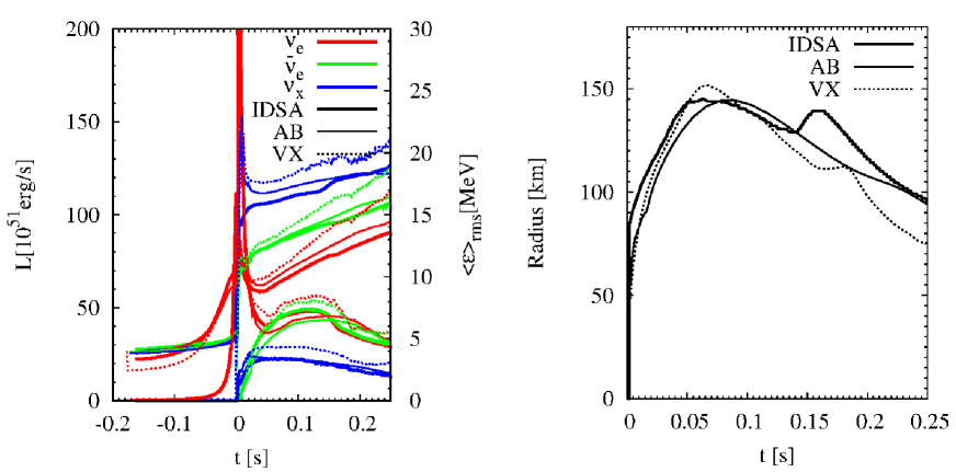
Figure 1: Left panel shows comparison of neutrino luminosities and rms energies as a function of postbounce time (similar to panel (b) in Liebendörfer et al. (2004)). The values are sampled at a radius of 500 km in the lab frame. The line width distinguishes between the results IDSA (thick lines), Agile-BOLTZTRAN (labeled as ”AB”, thin lines), and VERTEX (labeled as ”VX”, dotted lines). Thick red, green, and blue line denotes $\nu_{e}$, $\bar{\nu}_{e}$, and $\nu_{x}$, respectively. Same as the left panel, but the right panel shows comparison of the accretion shock front between IDSA (thick line), AB (thin line), and VX (dotted line).

From the left panel of Figure 1, one can see that the neutrino properties from IDSA are much closer to those in AB (Agile-BOLTZTRAN) than in VX (VERTEX). Here it should be emphasized that the higher neutrino luminosities and rms energies of VX are now lowered to meet closely with those of AB by changing the approximate GR treatment from Case R to Case A (Marek et al., 2006), the latter of which is employed in this work. In the sense, the qualitative agreement of the three codes is convincing, which we will explain more in detail below.

More quantitatively, the peak luminosity during the electron neutrino burst (red lines, out of the scale of the left plot) is higher by ($\sim 8\%$) for IDSA compared to that of AB ($L_{\nu_{e}}^{\rm peak}=3.3\times 10^{52}$ erg/s), whereas the half-width of the peak ($\sim 6$ ms) agrees well with each other. After the deleptonization burst, the luminosity of $\nu_{e}$ (red think line) and $\bar{\nu}_{e}$ (green thick line) of IDSA are higher (maximally by $10\%$) than those of AB till the first $\sim$ 160 ms after bounce. As already pointed out by Müller et al. (2010) and O’Connor (2015), this is most likely to come from the higher resolution at the shock front in the Eulerian codes compared to the Lagrangian code of AB. After the neutronization burst, the maximum luminosity of $\nu_{e}$ and $\bar{\nu}_{e}$ deviates maximally by $\sim 8\%$ between IDSA and AB. And the luminosity of each neutrino species between IDSA and AB points to a converged value towards the final simulation time (250 ms after bounce in this comparison).

The $\nu_{x}$ luminosity agrees quite well between IDSA (blue thick line) and AB (blue thin line) over the entire 250 ms postbounce. On the other hand, IDSA fails to reproduce the spike in the $\nu_{x}$ rms energy near bounce ($t\sim 0$) peaking at $\sim 24$ MeV, which is present in both AB and VX (blue thin and blue dotted line). This is one of the limitation of the IDSA scheme (M. Liebendörfer in private communication), which attempts to bridge the streaming and trapped neutrinos by the prescribed isotropic diffusion source term. For $\nu_{e}$ and $\bar{\nu}_{e}$, the neutrino sphere(s) is well defined as the decoupling surface from thermal equilibrium mediated by charged current interactions. The IDSA works well to capture this energy sphere. For $\nu_{x}$, on the other hand, not the energy sphere(s) but the scattering sphere(s) is the decoupling surface (Raffelt, 2012). In the transition region from the energy to scattering spheres, Doppler-shift terms (as well as the gravitational redshift) play an essential role in accurately determining the neutrino spectrum. By design, the IDSA (in the current form) cannot treat the highly complex transport phenomena appropriately. Moreover, the energy-redistribution in the neutrino phase space such as due to neutrino-electron scattering cannot be treated accurately in the current effective emissivity/absorptivity approaches (see Section 2.3). All of these simplifications should potentially lead to the missing of the spike in the $\nu_{x}$ energy near bounce.

The $\bar{\nu}_{e}$ (rms) energy (green thick line) is in good agreement with AB over the entire 250 ms, although IDSA underpredicts the $\nu_{e}$ energy (red thick line) by $\sim 6\%$ compared to AB. After bounce, IDSA underestimates the $\nu_{x}$ energy (blue thick line) by $\lesssim 10\%$ compared to AB till $\sim$ 160 ms after bounce, then matches closely to AB during the simulation time. The transition timescale ($\sim$ 160 ms) corresponds to the time when the silicon (Si)-rich shell accretes through the shock (e.g., middle left panel of Figure 5). This can be seen as a hump (solid black line) in the right panel of Figure 1, which leads to a drop in the $\nu_{e}$ and $\bar{\nu}_{e}$ luminosities (see red and green solid lines in the left panel). Note that the hump is missing in AB (right panel), which was due to the artificial diffusion introduced in the adaptive gridding of AB as already discussed in Liebendörfer et al. (2005).

More detailed code comparison not only between AB, VX, and IDSA, but also including Fornax (Skinner et al., 2016), FLASH (O’Connor & Couch, 2015), GR1D (O’Connor, 2015) codes is currently in progress (O’Connor et al. in preparation). We leave more detailed comparison to the forthcoming work. Given our approximate treatment of GR, neglect of energy-bin couplings, and the partial implementation of the Doppler-shift terms, it may not be surprising that IDSA has $10\%$ levels of mismatch with the full-GR and full-Boltzmann result of Agile-BOLTZTRAN. In fact, such discrepancies (given the use of similar level of approximation) has been also observed in the literature (e.g., O’Connor (2015); O’Connor & Couch (2015)). Having overviewed the validity and limitation of the current IDSA scheme, we shall move on to focus on the microphysical update in the following sections.

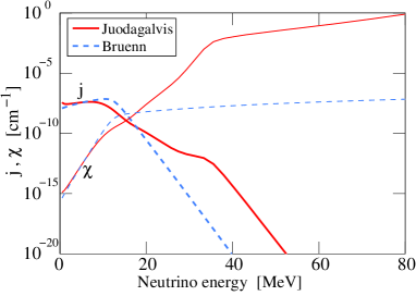
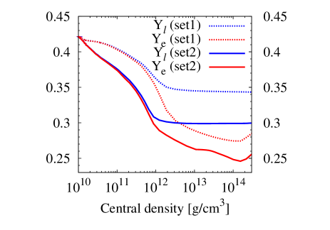
Figure 2: Left panel show comparison of emissivity ($j$) and absorptivity ($\chi$) of electron capture on heavy nuclei at a thermodynamic condition of $\rho=10^{11}\,{\rm g}~{}{\rm cm}^{-3},\,Y_{e}=0.45,T=10^{10}\,{\rm K}$ (corresponding to $\mu_{e}$ = 18.2 MeV) between the Bruenn rate (blue dashed line) and the rate by Juodagalvis et al. (2010) (red solid line), respectively. Here $\rho$, $T$, $Y_{e}$, and $\mu_{e}$ denotes density, temperature, electron fraction, and electron chemical potential, respectively. The absorptivity (equivalently $1/\lambda^{(a)}$ in Bruenn (1985), e.g., the Equation (C29)) is calculated by a detailed balance. The right panel shows comparison of $Y_{e}$ and lepton fraction ($Y_{l}$) as a function of the central density between set1 (dashed lines) and set2 (solid lines) using either the Bruenn or Juodagalvis rate, respectively.

3.2 Improved electron capture rate on heavy nuclei (set2)

We start to describe our first update in neutrino opacity, which is electron capture on heavy nuclei. Based on detailed shell-model calculations by Langanke & Martínez-Pinedo (2000), Langanke et al. (2003) showed that not only a generic $0f_{7/2}\rightarrow 0f_{5/2}$ Gamow-Teller (GT) transition, but also additional GT transitions, forbidden transitions, and thermal unblocking play a crucial role, which makes electron capture on heavy nuclei dominant over that on protons in the later phases in the core-collapse phase.

We employ a tabulated electron capture rate on heavy nuclei by Juodagalvis et al. (2010) who has extended significantly the covered mass range of nuclides ($\sim 2700$) compared to that of Langanke & Martínez-Pinedo (2000) ($\sim 100$). To calculate the needed abundances of the heavy nuclei, a Saha-like nuclear-statistical-equilibrium (NSE) is assumed. The table by Juodagalvis et al. (2010) then provides an average neutrino emissivity per heavy nucleus. Following Hix et al. (2003), one can calculate the full neutrino emissivity by the product of this average neutrino emissivity and the number density of heavy nuclei calculated by the employed EOS (here for LS EOS).

The left panel of Figure 2 compares the full neutrino emissivity/absorptivity ($j,\chi$, red solid line)) with that of the Bruenn prescription (blue dashed line, e.g., Equation (C27) of Bruenn (1985)) for a given thermodynamic condition in the core-collapse phase. From the panel, one can see a significant enhancement of the neutrino emissivity in the Juodagalvis rate (red solid line) compared to the Bruenn rate (blue dashed line) for neutrino energy above $\sim 18$ MeV. This high electron capture rate is also seen as a steeper slope in $\chi$ than that of the Bruenn rate ($\chi\propto\epsilon^{2}$ with $\epsilon$ representing the neutrino energy).

The right panel of Figure 2 compares $Y_{e}$ and lepton fraction ($Y_{l}$) as a function of the central density ($\rho_{c}$) between set1 (dashed line) and set2 (solid line) with the Bruenn or Juodagalvis rate, respectively. Deleptonization ends approximately at $\rho_{c}=2\times 10^{12}\,{\rm g}\,{\rm cm}^{-3}$, which marks onset of the neutrino trapping (Sato, 1975). The central $Y_{l}\sim 0.34$ at bounce (see at the right edge of blue dashed curve) using the Bruenn rate is lowered about $\sim 10\%$ ($Y_{l}\sim 0.3$, blue solid curve) with the Juodagalvis rate. For set1, the evolution of $Y_{e}$ and $Y_{l}$ matches quite nicely with AB Liebendörfer et al. (2005) (see their Figure 7(b)). For set2, our results are quantitatively very close to those of Hix et al. (2003) where the LMP rate (Langanke et al. (2003)) was implemented in the AB run using the same $15M_{\odot}$ progenitor model (Woosley & Weaver, 1995).

For making the comparison easy, Figure 3 and 4 are plotted in a similar way to Figure 1 and 2 in Hix et al. (2003) (see also Martínez-Pinedo et al. (2006)). Note that the LS180 was used in Hix et al. (2003), however, the differences with the difference $K$ of LS EOS are only a few percent around core bounce and less than $\sim 10\%$ in the first 200 ms after bounce (Thompson et al., 2003; Müller et al., 2010). So we consider that the different choice of $K$ does not significantly affect the aim of comparison here.

In fact, Figure 3 shows nice agreement with Figure 1 of Hix et al. (2003). From the top panel, the use of the improved electron capture rate leads to $\sim 10\%$ reduction in the central $Y_{l}$ and $Y_{e}$ compared to those with the Bruenn rate. The above match suggests that hydrodynamics impacts between the LMP and Juodagalvis rate should be fairly small. From the velocity profile (bottom panel), one can see that the mass of the unshocked, homologous core at bounce is reduced about $\sim 20\%$ from $\sim 0.62M_{\odot}$ for set1 (see discontinuety in the velocity plot) to $\sim 0.5M_{\odot}$ for set2. As already pointed out by Hix et al. (2003), the $10\%$ reduction of $Y_{l}$ leads to $\sim 20\%$ reduction in the homologous core because the (Chandrasekhar) mass of the unshocked core scales as $\langle Y_{l}\rangle^{2}$. The smaller entropy and central density (second and third panel in Figure 2) for set2 compared to set1 is also quantitatively consistent with Hix et al. (2003).

Figure 4 also supports correct implementation of the Juodagalvis rate in our code. The left panel shows that because of the enhanced electron capture rate and the resulting smaller radius at the shock formation (the bottom panel of Figure 3), the shock breakout is slightly delayed and the duration becomes slightly longer (a few ms) for set2 (red solid line) compared to set1 (dashed red line). In accordance with Hix et al. (2003), this feature is also seen in other neutrino flavors near core bounce ($\lesssim 50$ ms postbounce, see green and blue curves in the left panel). An overall trend in the rms neutrino energy (right panel of Figure 4) both in pre- and post-bounce phase is also in line with Hix et al. (2003); the $\nu_{e}$ rms energy is as much as $\lesssim$ 1 MeV smaller for set2 than set1 over the first 50 ms after bounce (compare red solid with red dashed line), but lower thereafter. The difference of $\bar{\nu}_{e}$ is minute compared to that of $\nu_{e}$.

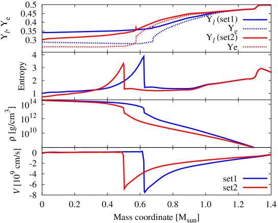
Figure 3: $Y_{e}$, entropy, density, and velocity profiles as functions of the enclosed mass at core bounce. The blue and red solid curve denotes the 1D run with the Bruenn rate (set1) or Juodagalvis rate (set2), respectively.

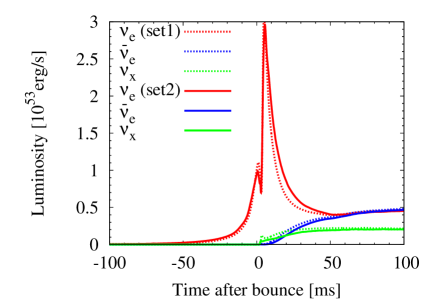
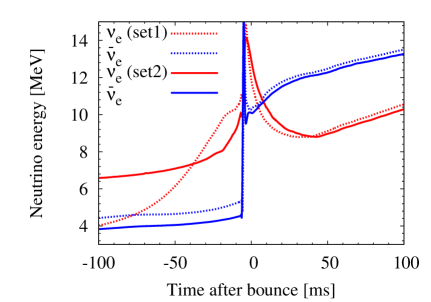
Figure 4: Comparison of the neutrino luminosity (left panel) and the rms energy (right panel) measured at a 500 km in the lab frame.

Figure 5 summarizes several key quantities for comparison between set1 and set2 over the first 500 ms after bounce. The top left panel shows that the largest difference is a $\lesssim 15\%$ reduction of $\nu_{x}$ luminosity of set2 (solid green line) compared to set1 (dashed green line) in the first $\sim$ 140 ms after bounce, but vanishes thereafter. The bottom left panel shows that the drop in the mass accretion rate ($\sim$ 140 ms) corresponds to the epoch when the Si-rich layer is passing through the shock. This leads to a dorm-like shape in the $\nu_{e}$ and $\bar{\nu}_{e}$ luminosity (see red and blue curves in the top left panel), the peak of which is at around the $\sim$ 140 ms after bounce. In the first 160 ms after bounce, the Si-rich layer has entirely passed though the shock as indicated by a low mass accretion in the bottom left panel. At this phase, one can see the $\sim 5\%$ reduction of the $\nu_{e}$ and $\bar{\nu}_{e}$ luminosity in set2 compared to set1. The rms energy (top right panel) for all the neutrino flavors becomes smaller (maximally by $\sim$ 0.4 MeV) in set2 (solid lines) compared to set1 (dashed line). The smaller homologous mass at bounce for set2 could potentially lead to smaller gravitational energy release in the postbounce phase compared to set1, which is reconciled with the above trends. The bottom right panel shows that the net heating rate for set2 (red line) is smaller by $\lesssim 7\%$ compared to set1 (blue line).

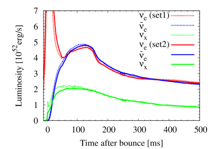
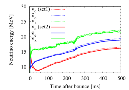
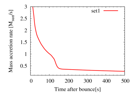
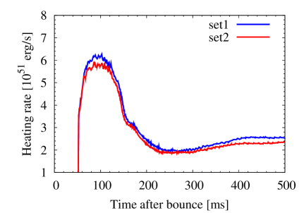
Figure 5: Comparison of several key quantities in 1D simulations with neutrino physics set1 or set2. In the top panels, we show the neutrino luminosities (left) and the neutrino rms energy (right) measured at a radius of 500 km in the lab frame. The bottom left panel shows the mass-accretion rate evaluated at 500 km. The bottom right panel compares the net heating rate integrated over the gain region.

Regarding the update in this section, one would imagine from the 1D comparison that the improved electron capture rate on nuclei might weaken ”explodability” in multi-D simulations. The readers would see whether this expectation is correct or not in Section 4 (2D results).

3.3 Electron Neutrino Pair Annhilation (set3a) and $\nu_{x}+\nu_{e}(\bar{\nu}_{e})$ Scattering (set3b)

In this section, we first focus on set3a (see Table 1) where electron neutrino pair annhilation process ($\nu_{e}+\bar{\nu}_{e}\rightleftharpoons\nu_{x}+\bar{\nu}_{x}$, for short, we call this as the ”nupair” process in this section) is added to set1. Buras et al. (2003) were the first to point out that as a source for $\nu_{x}$ the nupair reaction is always more important than the traditional electron-positron pair annihilation process ($e^{-}\,e^{+}\rightleftharpoons\nu_{x}\,\bar{\nu}_{x}$, for short, we call this as the ”eepair” process in the following). The implementation scheme of the nupair process in IDSA is given in Appendix A.

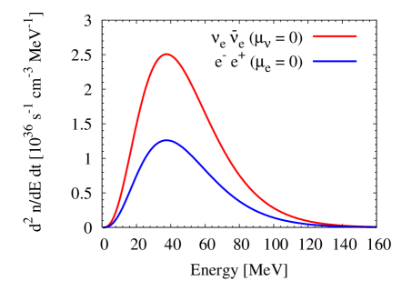
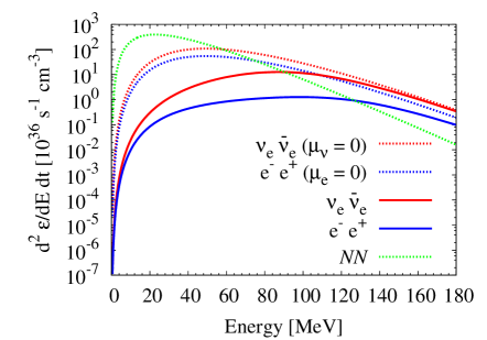
Figure 6: The left panel compares neutrino-pair production number spectra (Equation (A12)) as a function of neutrino energy for $T=12$ MeV between the nupair and eepair process. Note that the chemical potential for electron and neutrinos is set to zero ($\mu_{e}=0$ and $\mu_{\nu}=0$), corresponding to Figure of Buras et al. (2003) (but with a different scale in the $y$ axis). The right panel shows energy production rates (Equation (A13)) for the nupair and eepair processes including nucleon-nucleon Bremsstrahlung (labeled as ${\it"NN"}$ in the panel). For the right panel, the following thermodynamic condition is chosen as $\rho=5\times 10^{13}\,\rm{g}/\rm{cm}^{-3}$, $Y_{e}=0.3$, $T=12$ MeV, (corresponding to $\mu_{e}=96$ MeV and $\mu_{\nu_{e}}=123$ MeV), respectively. The right panel corresponds to Figure 16a of Fischer et al. (2009), where some typos in the label of $y-$axis is now corrected. Note in both of the panels that the final state Pauli blocking is neglected.

In fact, the left panel of Figure 6 clearly shows the dominance of the nupair process (red solid line, labeled as ”$\nu_{e}\bar{\nu}_{e}$”) over the eepair process (blue solid line, labeled as ”$e^{-}e^{+}$”). In this panel, the chemical potential for electron and neutrinos is set to zero ($\mu_{e}=0$ and $\mu_{\nu}=0$), following Figure 3 of Buras et al. (2003). The peak in the spectra of the nupair process is about two times higher than that of the eepair process at the neutrino energy of $\sim 40$ MeV. As explained in Buras et al. (2003), this simply comes from the different weak coupling constants between the two processes. The production kernels have a similar form as, $\Phi^{p}=(C_{\rm V}+C_{\rm A})^{2}J^{I}+(C_{\rm V}-C_{\rm A})^{2}J^{II}$ (e.g., Equation (C63) in Bruenn (1985)). For the eepair process, $C_{\rm V}=-1/2+2\sin^{2}\theta_{w}$ and $C_{\rm A}=-1/2$ (with the weak mixing angle; $\sin^{2}\theta_{w}=0.23$), whereas $C_{\rm V}=1/2$ and $C_{\rm A}=1/2$ for the nupair process. Given that $J^{I}\sim J^{II}$, the two-times difference can be readily seen by putting these numbers in the above equation of $\Phi^{p}$.

The right panel of Figure 6 shows comparison between the energy production rates with (solid lines) and without chemical potentials (dashed lines, labeled with $\mu_{\nu}$ = 0, $\mu_{e}$ =0). As a reference, the production rate of nucleon-nucleon Bremsstrahlung is also shown (labeled as ${\it"NN"}$). In accordance with Fischer et al. (2009), the chemical potentials make the spectra harder and the rate smaller. Quantitatively, the $\eta$-paramter of $\sim 10$ in the right panel (e.g., for electron, $\eta_{e}=\mu_{e}/T=\sim 96{\rm MeV}/12{\rm MeV}=8$, and electron-neutrino, $\eta_{\nu_{e}}=\mu_{\nu_{e}}/T=\sim 123{\rm MeV}/12{\rm MeV}\sim 10$). This leads to $\gtrsim 1/10$ reduction in the rates with the chemical potential than those without. This is consistent with Buras et al. (2003) (their Figure 2). Comparing to Figure 16a of Fischer et al. (2009), the peak energy of Bremsstrahlung is around $\sim 30$ MeV, and the specral shape matches well together.

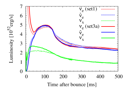
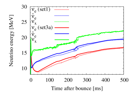
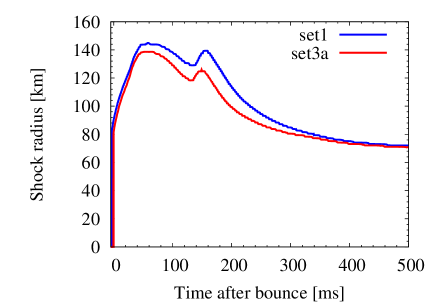
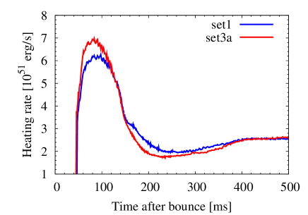
Figure 7: Same as Figure 5 but for the comparison between set3a and set1. The bottom left panel compares the shock evolution.

The top left panel of Figure 7 compares the neutrino luminosities between set3a (solid lines) and set1 (dashed lines). Before the first 160 ms after bounce when the mass accretion rate is still high (e.g., the bottom left panel of Figure 5), the influence of the nupair process is biggest for the $\nu_{x}$ luminosity ($\lesssim 20\%$ increase from set1, compare green solid with green dashed line), followed in order by the $\nu_{e}$ luminosity ($\sim 4\%$ increase, compare red solid line with red dashed line) and by the $\bar{\nu}_{e}$ luminosity ($\lesssim 2\%$ increase, blue solid line with blue dashed line). Using the same $15M_{\odot}$ progenitor, this is quantitatively very close to the results in Buras et al. (2003) (see their Figure 7). As is consistent with Buras et al. (2003) and Fischer et al. (2009), the additional source of $\nu_{x}$ increases the $\nu_{x}$ luminosity most significantly. In the accretion phase ($\lesssim 160$ ms postbounce), the nupair process also leads to higher rms neutrino energies (top right panel of Figure 7). This is due to the enhanced cooling which makes the positions of the neutrino spheres and the PNS formed deeper inside (e.g., Figure 17 of Fischer et al. (2009) of the corresponding Agile-BOLTZTRAN run but for a $40M_{\odot}$ star). After the accretion phase ($\gtrsim 160$ ms postbounce), the luminosities of $\nu_{e}$ and $\bar{\nu}_{e}$ become smaller than those in set1 (top left panel of Figure 7), As already pointed out by Buras et al. (2003), this is most likely because of the more compact neutrino spheres (e.g., smaller emission region) in response to the more accelerated PNS contraction. The (maximum) shock position of set3a is more compact compared to set1 by $5\sim 10\%$, which is within the change seen in Buras et al. (2003) and Fischer et al. (2009). From the bottom right panel of Figure 7, it is interesting to note that the net heating rate of set3a (red line) dominates over that of set1 (blue line) in the accretion phase ($\lesssim 160$ ms postbounce), which reverses thereafter (until $\sim 400$ ms postbounce). This is in line with the higher (and lower) luminosities of $\nu_{e}$ and $\bar{\nu}_{e}$ of set3a compared to set1 in the pre- and (post-) accretion phase, respectively as already mentioned above.

As originally pointed out by Buras et al. (2003), the cross channel of the nupair process, that is $\nu_{x}+\nu_{e}/\bar{\nu}_{e}\rightleftharpoons\nu_{x}+\nu_{e}/\bar{\nu}_{e}$, could be of comparable importance to $\nu_{x}+e^{\pm}$ scattering. The top and bottom left panel of Figure 8 compares the (inverse) mean free path of $\nu_{e}+e^{-}$ scattering (red line), $\nu_{x}+e^{-}$ scattering (blue line), and $\nu_{x}+\nu_{e}$ scattering (green line) for typical thermodynamics conditions in the supernova core, respectively. Note that the corresponding reactions with $\bar{\nu}_{e}$ and $e^{+}$ are not shown in the panels because they are much smaller compared to those with $\nu_{e}$ and $e^{-}$. In the prebounce phase, the top panels of Figure 8 show that $\nu_{x}\nu_{e}$ scattering (green line) is almost comparable to $\nu_{x}e^{-}$ scattering (blue line). But they play a minor role as a opacity (in the leptonic channels) because of the dominant contribution from $\nu_{e}\,e^{-}$ scattering (red line). In the postbounce phase (bottom left panel of Figure 8), the dominance of $\nu_{e}\,e^{-}$ scattering is also unchanged, but the opacity of $\nu_{x}e^{-}$ scattering becomes higher than that of the $\nu_{x}\nu_{e}$ scattering, as previouly shown in Buras et al. (2003).

The bottom right panel of Figure 8 compares the neutrino luminosities between set3a (dashed line) and set3ab (solid line). Note that set3ab is the run where neutrino-scattering scattering is added to set3a. The solid and dashed lines are completely overlapped, which confirms the expectation that $\nu_{x}\nu_{e}$ scattering plays a very minor role at least over the first 500 ms postbounce.

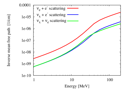
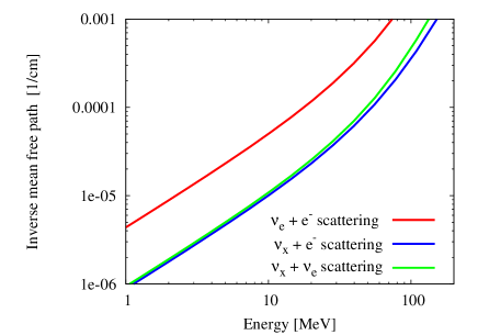
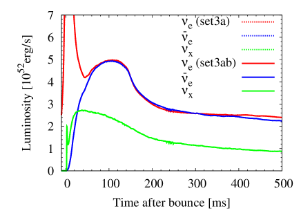
Figure 8: Inverse mean free path (e.g., Equation (B4)) as a function of neutrino energy for three typical conditions; near neutrino trapping (top left, $\rho=10^{12}\,{\rm g}\,\,{\rm cm}^{-3}$, $T=1.76$ MeV, and $Y_{e}=0.35$), near core bounce (top right panel, $\rho=3\times 10^{14}\,{\rm g}\,\,{\rm cm}^{-3}$, $T=12$ MeV, and $Y_{e}=0.27$), and in the postshock region behind the shock (bottom left panel, $\rho=1\times 10^{12}\,{\rm g}\,\,{\rm cm}^{-3}$, $T=7$ MeV, and $Y_{e}=0.10$), respectively. Here Fermi-Dirac final state neutrino distributions are assumed. The bottom right panel compares the neutrino luminosities between set3a and set3ab. Note that set3ab is the model where $\nu_{x}+\nu_{e}(\bar{\nu}_{e})$ scattering is added to set3a.

3.4 Mean-field modifications (set4a and set4b)

Martínez-Pinedo et al. (2012) and Roberts et al. (2012) clearly pointed out that medium effects (Reddy et al., 1998) affect differently protons and neutrons (e.g., the reactions of set4a in Table 1), leading to a significant impact on the neutrino luminosities and spectra especially in the PNS cooling phase (after the onset of an explosion). By definition, our (non-exploding) 1D simulation can cover only a pre-explosion phase. Having in mind future applications for a long-term evolution in multi-D (exploding) models, we explore in this section the impact of the mean-field corrections on the charged-current opacities treated at the elastic level (Martínez-Pinedo et al. (2012); Roberts et al. (2012)).

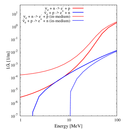
Figure 9: Inverse mean free path as a function of neutrino energy for $\nu_{e}$ (red line) and $\bar{\nu}_{e}$ (blue line) with (dashed lines, labeled with ”in-medium”) and without (solid lines) mean-field corrections. A thermodynamics condition of $T=8$ MeV, $n_{B}=0.02\,{\rm fm}^{-3}$, $Y_{e}=0.027$ is chosen with $n_{B}$ the baryon number density, which corresponds to Figure 3 of Roberts et al. (2012). Note that the nucleon potential difference is $\Delta U=9$ MeV for the EOS used in Roberts et al. (2012), whereas $\Delta U=7.67$ MeV for LS220 in this work, leading to a slight difference quantitatively.

From Equation (3) of Martínez-Pinedo et al. (2012), the opacity of $\nu_{e}$ absorption on neutron ($\nu_{e}\,n\rightarrow e^{-}\,p$) is expressed as,

$$\frac{1}{\lambda_{\nu_{e}}}\propto E_{e}^{2}[1-f_{e}(E_{e})]\frac{n_{n}-n_{p}}{1-\exp{\beta(\mu^{0}_{p}-\mu^{0}_{n}+\Delta U)}},$$ (7)

where $E_{e}$ is the electron energy, $f_{e}$ is the electron distribution function, $n_{i}$ and $\mu^{0}_{i}$ is the number density and chemical potential (without rest mass) for $i=n,p$ (neutrons and protons) and $\beta$ is the inverse temperature, respectively. At the level of an elastic approximation (Reddy et al., 1998; Martínez-Pinedo et al., 2012), the following relation holds

$$E_{e}=E_{\nu_{e}}+Q+\Delta U,$$ (8)

where $E_{\nu_{e}}$ is the $\nu_{e}$ energy, $Q=m_{n}-m_{p}$ is the so-called $Q$ value with $m_{i}$ the rest mass for $i=n,p$, and $\Delta U=U_{n}-U_{p}$ is the difference of the mean-field potentials of neutrons and protons.

From Equation (8), $E_{e}^{2}$ in Equation (7) becomes larger due to $\Delta U$, which leads to increase in the $\nu_{e}$ opacity comparing to the free gas case ($\Delta U=0$) at lower neutrino energies. At larger neutrino energies, the Pauli blocking disappears, which makes the opacity with and without the mean-field effects approach each other closely (e.g., Martínez-Pinedo et al. (2014) for more detail). For $\bar{\nu}_{e}$, the positron energy becomes $E_{e^{+}}=E_{\bar{\nu}_{e}}-Q-\Delta U$. This leads to the reduction of the opacity at lower neutrino energies. Note also that the $Q$ value of this reaction increases from $E_{\bar{\nu}_{e}}>Q$ to $E_{\bar{\nu}_{e}}>Q+\Delta U$.

Figure 9 is consistent with the above explanations, which compares the inverse mean free path for $\nu_{e}$ (red lines) and $\bar{\nu}_{e}$ (blue lines) with (dashed lines) and without the mean-field corrections (solid lines). These features are also in good agreement with previous work (e.g., Roberts et al. (2012) and Martínez-Pinedo et al. (2012)).

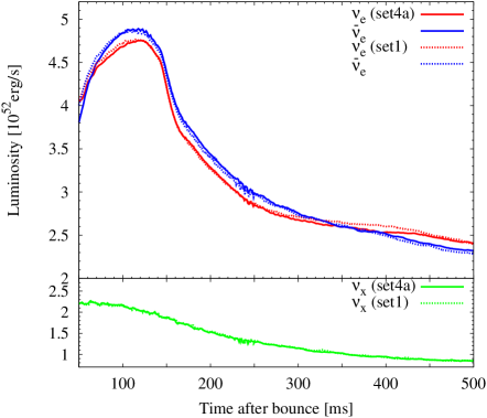
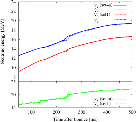
Figure 10: Comparison of $\nu_{e}$ and $\bar{\nu}_{e}$ luminosities and the rms energies (upper part of the panels) and those of $\nu_{x}$ (lower part of the panels) between set4a (solid lines) and set1 (dashed lines), respectively.

The upper panels of Figure 10 compare the $\nu_{e}$ and $\bar{\nu}_{e}$ luminosities (left panel) and the rms energies (right panel) between set4a (solid lines) and set1 (dashed lines), respectively. After the accretion phase ($\sim 160$ ms after bounce), the $\bar{\nu}_{e}$ luminosity for set4a (blue solid line) becomes slightly larger (by $\lesssim 1\%$) compared to that of set1 (blue dashed line). More apparent difference can be seen by comparing the $\nu_{e}$ luminosity of set4a (red solid line) that of set1 (red dashed line) (approximately $3\sim 4\%$ lower for set4a). First of all, these features are consistent with the reduction of the $\bar{\nu}_{e}$ opacity (leading to higher $\bar{\nu}_{e}$ luminosity) and the increase of the $\nu_{e}$ opacity (lower $\nu_{e}$ luminosity) due to the mean-fields effects, as we mentioned above. Regarding the rms neutrino energies (right panel), the mean-field effects increase the $\bar{\nu}_{e}$ energy by $\sim 20\%$, but barely affect the $\nu_{e}$ energy, also the $\nu_{x}$ luminosities and the rms energy (compare green solid lines with green dashed lines).

The bigger mean-field effects observed in this study, such as on the $\nu_{e}$ luminosity compared to the $\bar{\nu}_{e}$ luminosity, the same as for the $\bar{\nu}_{e}$ rms energy compared to the $\nu_{e}$ rms, are consistent with Horowitz et al. (2012). Note that Horowitz et al. (2012) observed more stronger impact of the mean-field effects, especially on the increase of the $\bar{\nu}_{e}$ rms energy and the reduction of the $\nu_{e}$ luminosity (see their Figure 4). The employed progenitor (15 $M_{\odot}$) and the EOS (LS220) are the same as those in this work. However, the quantitative differences from Horowitz et al. (2012) could originate from their use of $\Delta U$ obtained by a virial expansion calculation (not from the LS220 EOS as in this work), the inclusion of the weak magnetism correction (not included in our set4a and set1), and the GR hydrodynamics (essentially Newtonian hydrodynamics in this work).

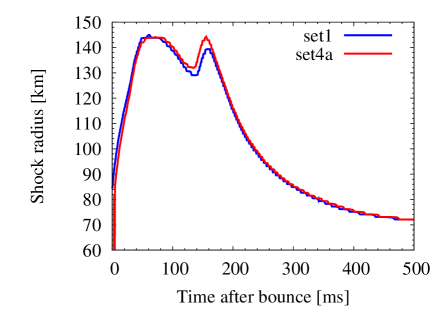
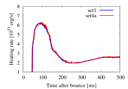
Figure 11: Comparison of the shock radius (left panel) and the net heating rate in the gain region (right panel) for set1 and set4a, respectively.

The left panel of Figure 11 compares the shock radius between set4a and set1. The shock radius becomes slightly bigger for set4a (red line) compared to set1 (blue line) for a short period ($\sim 120-160$ ms after bounce) when the Si-rich layer is advecting through the shock, but the difference disappears thereafter. Note in the period that the $\bar{\nu}_{e}$ luminosity is bigger than the $\nu_{e}$ luminosity (left panel of Figure 10). As mentioned above, the mean-field effects of set4a lead to higher $\bar{\nu}_{e}$ luminosity than set1, which is consistent with the bigger shock radius, albeit transietnly.

The right panel of Figure 11 compares the net heating rate in the gain region, suggesting that the mean-field effects, as previously reported (e.g., Martínez-Pinedo et al. (2012); Horowitz et al. (2012)), would not have a significant impact on the onset of an explosion. Similar comparison between set4b and set1 shows that the difference from set1 due to the in-medium suppression of Bremsstrahlung (see Table 1) is much smaller comparing to the mean-field effects mentioned above. The comparison plots between set4b (not shown) and set1 are almost completely overlayed (like in the middle left panel of Figure 12 or in the bottom right panel of Figure 8). It was shown (e.g., Fischer (2016) and Bartl et al. (2016)) that the medium suppression of Bremsstrahlung affects the neutrino properties only clearly after the onset of an explosion and the following PNS cooling phase. In this respect, our results showing a negligle impact in the pre-explosion phase are in line with the literature.

3.5 Weak Magnetism and Recoil (set5a), Nucleon Effective Mass (set5b)

In order to take into account the effects of weak magnetism and recoil both on the charged current (CC) and neutral current (NC) reactions, we follow Horowitz (2002) (their Equations (22) and (32)). The top left panel of Figure 12 correpsonds to Figure 1 (Horowitz, 2002), showing that the main effect from weak magnetism is to reduce $\bar{\nu}_{e}$ opacity (solid line) by a large amount ($\sim 15\%$ reduction at a neutrino energy of 20 MeV). In comparison, the $\nu_{e}$ opacity is enhanced only by a small amount (dashed line). Regarding NC reactions, Figure 2 of Horowitz (2002) shows that the reduction of the opacity is slightly higher for $\nu p$ scattering than $\nu n$ scattering, and that the reduction of the $\bar{\nu}$ reactions is higher than the corresponding $\nu$ reactions ($\sim 10\%$ reduction for $\bar{\nu}$ at a neutrino energy of 20 MeV).

The top right panel of Figure 12 compares the neutrino luminosities between set5a (solid lines) and set1 (dashes line) with and without weak magnetism and recoil, respectively. One can clearly see the enhancement of the $\bar{\nu}_{e}$ luminosity (blue solid line) for set5a, which is by $\sim 8\%$ bigger than set1 (blue dashed line). This comes from the reduction of the $\bar{\nu}_{e}$ opacity as mentioned above. The difference, however, becomes very small after $\sim 340$ ms postbounce. The $\nu_{e}$ luminosities (red solid line and red dashed line) are hardly affected, which is in line with the very small change in the $\nu_{e}$ opacity. The $\nu_{x}$ luminosity (green solid line and green dashed line) is enhaced up to about $\sim 10\%$ for set5a compared to set1. Regarding the rms neutrino energies (middle right panel), the reduced opacities of $\bar{\nu}_{e}$ and $\nu_{x}$ result in the higher $\bar{\nu}_{e}$ (blue solid line) and $\nu_{x}$ energies (green solid lines) up to $\sim 1$ MeV, comparing to those of set1 (blue dashed line and green dashed line).

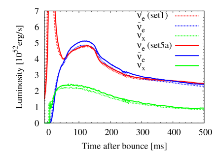
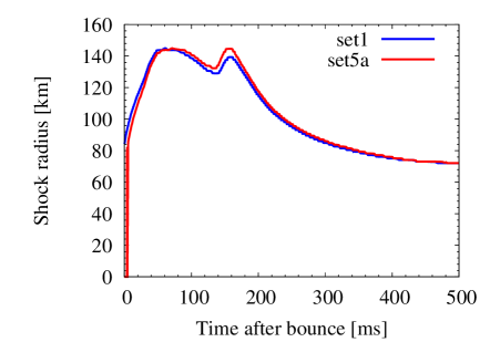
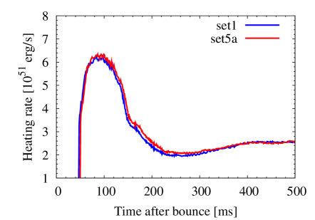
Figure 12: The top left panel shows the correction factor of the charged current cross section for $\nu_{e}$ (dashed line) and $\bar{\nu}_{e}$ (solid line) including weak magnetism and recoil as a function of neutrino energy. Note that except for middle left panel (showing a negligible difference from set5b and set1), the other panels are comparison between set5a and set1.

From the bottom left panel of Figure 12, one can see that the shock radius of set5a is transiently bigger than set1 for the epoch when the Si-rich shell is passing. This is most likely to come from the higher $\bar{\nu}_{e}$ luminosity and energy (top right and middle right panel). In fact, the net heating rate is slightly higher for set5a (red line) compared to set1 (blue line) up to the first $\sim 340$ ms after bounce. Thereafter, the $\bar{\nu}_{e}$ luminosity with and without weak magnetism correction approach each other together (top right panel). Set5b (effective mass correction, e.g., Table 1) does not exhibit visible changes from set1 (as was the case for set3b and set4b), only the comparison plot of the neutrino luminosities (middle left panel) is shown as a reference.

3.6 Quenching of $g_{a}$ (set6a), Many-body Effect (set6b), Strangeness Contribution (set6c), and the Whole Set

Finally, the model series with ”set6” include modifications to the axial-vector currents in the weak interactions either from the in-medium effects (set6a), many-body effects (set6b), or strangeness-dependent contributions (set6c), respectively (see Section 2.2 and Table 1 for details).

From the top panels of Figure 13, it is very hard to see significant differences between set6a and set1. This suggests that the quenching of $g_{a}$ plays a negligible role in the first 500 ms after bounce covered in our 1D run. For set6b, the left middle panel shows that the $\nu_{x}$ luminosity is higher by $\sim 10\%$ (green solid line) compared to set1 (green dashed line). The relative difference becomes larger in the later postbounce phase predominantly because the many-body effects reduce the opacity of the $\nu N$ scattering at high densities (Horowitz et al., 2017). This is also the case for the $\nu_{e}$ and $\bar{\nu}_{e}$ luminosities, where the luminosities become higher by $\sim 3-4\%$ for set6b toward the final simulation time. The clearer impact of the many-body effects on $\nu_{x}$ compared to $\nu_{e}$ and $\bar{\nu}_{e}$ is also seen in the middle right panel, showing an increase of $\sim 1$ MeV in the $\nu_{x}$ energy for set6b (green solid line) comparing to set1 (green dashed line).

The bottom left panel of Figure 13 shows a clear increase of the $\nu_{e}$ and $\bar{\nu}_{e}$ luminosities (by $\sim 4\%$) for set6c compared to set1 in the first $\sim$ 160 ms after bounce. At this epoch, the increase in the $\nu_{x}$ luminosity is more bigger ($\sim 9\%$). The bottom right panel shows that the strangeness effects lead to a slight increase in the rms neutrino energies where the maxium upshift is $\sim 0.2$ MeV in the $\nu_{x}$ energy (green solid line and green dashed line). These trends with the strangess contribution are qualitatively consistent with Melson et al. (2015a). In the 3D full-scale simulations by Melson et al. (2015a), they observed much bigger effects from the strangeness effects, such as $\sim 30\%$ and $10-15\%$ increase in the $\nu_{x}$ and $\nu_{e}$/$\nu_{e}$ luminosity, respectively, and $\sim 1$ MeV increase in the mean neutrino energies. Note in Melson et al. (2015a) that the use of the larger value of $g^{s}_{a}=-0.2$ and the choice of the more massive progenitor with the higher mass accretion rate (a $20M_{\odot}$ star) could potentially lead to the more clearer impact of the strangeness effect comparing to those in this work (see also Bollig et al. (2017) for 2D results using $g^{s}_{a}=-0.1$).

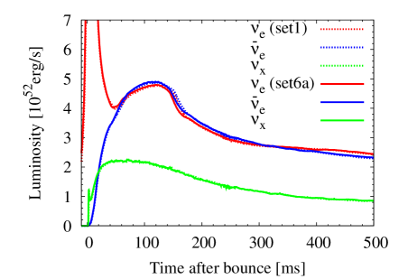
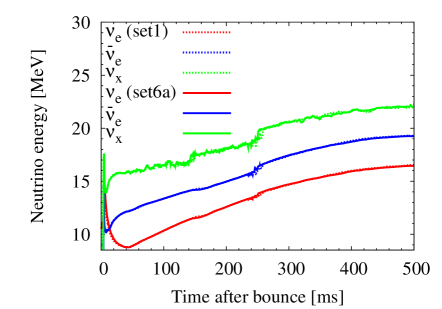
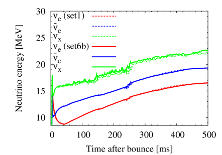
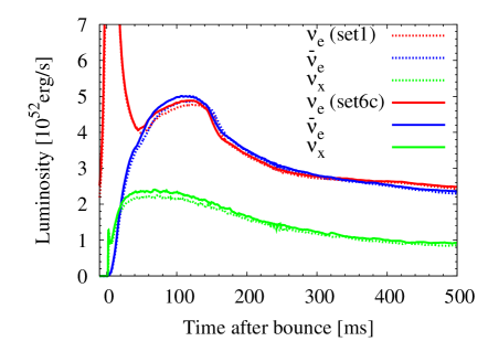
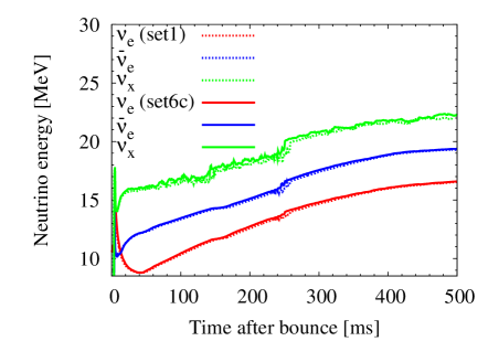
Figure 13: Comparison of the neutrino luminosities (left panels) and rms neutrino energies (right panels) between the set6 series (solid lines) with set1 (dashed lines), respectively.

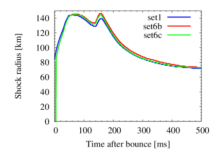
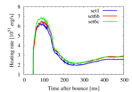
Figure 14: Comparison of the shock radius and the net heating rate in the gain layer between set6b, set6c, and set1, respectively. Note that set6a is not shown because of the overlap with set1, which makes the differences in the plots difficult to see.

The top left panel of Figure 14 shows that maximum shock extent becomes by $\sim 5\%$ bigger for set6b and set6c compared to set1 near the hump region ($\sim 160$ ms after bounce). The mentioned higher $\nu_{e}$ and $\bar{\nu}_{e}$ luminosities in the accretion phase (e.g., Figure 13) is in line with this feature. In fact, the right panel of Figure 14 shows that the net heating rate for set6b (red line) and set6c (green line) is bigger than that of set1 (blue line). For set6b, the increase from set1 (blue line) is about $\sim 6\%$ around 100 ms after bounce and higher at later times. This is in good agreement with Horowitz et al. (2017) (see their Figure 3). Regarding the strange-quark contribution, the heating rate (set6c, green line) becomes larger by $\sim 12\%$ than that of set1. This is in accordance with Horowitz et al. (2017). Note that significantly bigger impact ($\sim 20\%$ increase) was observed in Horowitz et al. (2017) probably because of the larger value of $g^{s}_{a}=-0.2$ and the use of a more massive 20 $M_{\odot}$ progenitor.

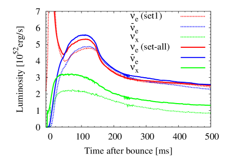
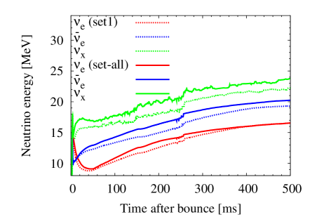
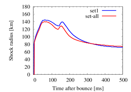
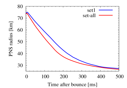
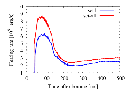
Figure 15: Similar to Figure 5 but for the comparison between set-all and set1. Note that set-all includes all of the updates to set1 (from set2 to set6c in Table 1).

Finally, Figure 15 compares the model including all of the updates to set1 (from set2 to set6c in Table 1, labeled as ”set-all” in the panels) with set1. Comparing with set1, the top left panel shows that the largest increase of the neutrino luminosities is for $\nu_{x}$ (by $\sim 31\%$), which is followed in order by $\bar{\nu}_{e}$ ($\sim 14\%$) and $\nu_{e}$ ($\sim 11\%$). Among the individual updates, the increase of the $\nu_{x}$ luminosity is biggest ($\sim 20\%$) due to the inclusion of electron neutrino pair annhilation (set3a) as shown in the top left panel of Figure 7. Note that the increase from the weak magnetism and recoil is $\sim 10\%$ in set5b (top right panel of Figure 12), from the many-body effects is $\sim 8\%$ in set6b (middle left panel of Figure 13), and $\sim 9\%$ from the strangeness contribution (middle left panel of Figure 13). As is expected, by adding the contribution from these individual rates (for the $\nu_{x}$ luminosity) does not simply explain the total increase ($\sim 31\%$). This is not surprising because the individual update affects non-linearly the postbounce evolution that is governed by non-linear neutrino-radiation hydrodynamics.

The $\bar{\nu}_{e}$ luminosity is bigger ($\sim 5.4\%$) than the $\nu_{e}$ luminosity at the peak around 100 ms after bounce, thereafter the difference becomes smaller towards the final simulation time. As already seen from Figure 12 (top left panel), the dominance of the $\bar{\nu}_{e}$ over the $\nu_{e}$ luminosity is mainly due to the inclusion of the weak magnetism and recoil (set5a). Using the same 15$M_{\odot}$ progenitor (Woosley & Weaver, 1995), this feature is also seen in Müller & Janka (2014) (see their Figure 1, the panel labeled with ”s15s7b2”), where neutrino signals from 2D GR simulations using the Vertex-CoCoNuT code were investigated. In Müller & Janka (2014), the main difference regarding the microphysics inputs from this work is the use of LS180 EOS and the inclusion of the non-elastic effects in the charged current absorption reactions (Burrows & Sawyer, 1998, 1999). The energy-redistribution from the latter would make the recoil effect smaller, which would explain the smaller difference between the $\bar{\nu}_{e}$ and the $\nu_{e}$ luminosity in Müller & Janka (2014). Their 2D run of the 15$M_{\odot}$ star (G15) starts to explode at $\sim 570$ ms after bounce and the postbounce dynamics deviates from 1D after around 100 ms after bounce (Müller et al., 2013). At the 100 ms after bounce, their $\nu_{e}$ and $\bar{\nu}_{e}$ luminosity is $\sim 5\times 10^{52}$ erg/s, which is slightly lower than those in this study $\sim 5.3-5.6\times 10^{52}$ erg/s. Note that the neutrino luminosities in Müller et al. (2013) take into account the GR effects (their Equation (2) and (3)), which could potentially lead to $\sim 10-20\%$ reduction comparing to those without the GR corrections. Regarding the $\nu_{x}$ luminosity, the peak value is $\sim 2.4\times 10^{52}$ erg/s in Müller et al. (2013), which is ($\sim 25\%$) lower than that in this work. Although we do not have a clear-cut answer, we consider that the reduction of the $\nu_{x}$ luminosity due to the GR redshift effects could partly explain the discrepancy. This is because the neutrinospheric radii of $\nu_{x}$ are formed deeper inside where the GR correction becomes more significant among the other neutrino species.

The top right panel of Figure 15 shows that all the rms neutrino energies become higher for set-all (solid lines) than set1 (dashed lines) over the first 500 ms after bounce. The enhancement due to the updated opacity is bigger for $\nu_{x}$ and $\nu_{e}$ by $\sim$ 2 MeV compared to $\nu_{e}$ by $\sim 1$ MeV. Note in Müller et al. (2013) that not the rms but the mean neutrino energy was plotted. At the 100 ms after bounce, the mean energy is (probably incidentally) very close, $\nu_{e}$, $\bar{\nu}_{e}$, and $\nu_{x}$ is $\sim 9$ MeV, $\sim 13$ MeV, and $\sim 15$ MeV in Müller et al. (2013), which is $\sim 10$ MeV, $\sim 13$ MeV, and $\sim 15$ MeV in our work, respectively.

The middle left panel of Figure 15 shows that the shock position when the bounce shock stalls (at 100 ms after bounce) is $\sim 3\%$ smaller for set-all (red line) compared to set1 (blue line). At the hump that marks the passing of the Si-rich layer through the shock ($\sim 160$ ms after bounce), the difference of the shock between set-all and set1 becomes largest $\sim 9\%$. After $\sim$ 300 ms postbounce, the two shock radius approaches very close, but the shock radius of set-all becomes as big as $\sim 5\%$ compared to set1 toward the final simulation time. The enhanced $\nu_{e}$ and $\bar{\nu}_{e}$ luminosities due to the many-body effects (set6b, see the middle left panel after $\sim$ 300 ms postbounce) and the extended shock radius (red line in the left panel of Figure 14) is reconciled with the above features seen in set-all. The middle right panel of Figure 15 shows the more compact PNS radius for set-all (red line) compared to set1 (blue line). Note that the PNS radius is estimated at a fiducial density of $10^{11}\,{\rm g}\,{\rm cm}^{-3}$. The difference is biggest at the hump seen in the shock evolution ($\sim 160$ ms after bounce), when the PNS radius is smaller by $\sim 17\%$ for set-all relative to set1. Although the difference becomes smaller toward the final simulation time, the PNS radius is always smaller for set-all over the entire 500 ms after bounce.

The bottom panel of Figure 15 shows that the maximum enhancement of the net heating rate of set-all (red line) is $\sim 30\%$ compared to set1 (blue line) at around 100 ms after bounce. After the 160 ms postbounce, the net heating rate in the gain region becomes $\sim 10-24\%$ higher for set-all. This is predominantly because of the higher $\bar{\nu}_{e}$ and $\nu_{x}$ luminosities and rms energies (top left and right panels) and of the smaller PNS radius (middle right panel). As already discussed above, the improved opacities add non-linearly and synergetically to increase the net heating rate, where each of the individual update amounts to the $\lesssim 10\%$ level (e.g., see Figures 5 to 14).

4 2D Results

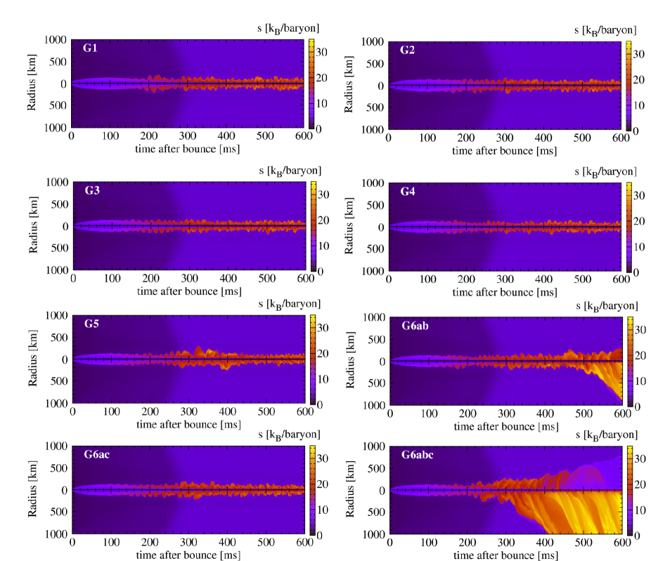
Figure 16: Entropy along the north and south polar axis a postbounce time for the 2D simulations of G1 to G6abc (from top left to bottom panel). The shock trajectory can be seen as a discontinuity between the dark violet and blue tones in the pre-shock region and light colors (red, orange, yellow) in the post-shock region. Here entropy is in the unit of $k_{B}^{-1}\,{\rm nucleon}^{-1}$ with $k_{B}$ the Boltzmann constant.

In this section, we present results of our 2D core-collapse simulations where selected sets of the neutrino opacities in Table 1 are included in set1. As already mentioned in Section 2.1, we choose a 20$M_{\odot}$ star (Woosley & Heger, 2007) in our 2D runs.

Our 2D run with the Bruenn rate (set1) is now called ”G1” (meaning group one). ”G2” is the model that is equivalent to set2 in the previous section. ”G3” is the model where set3a and set3b are added to G2. Like this, for ”G4”, set4a and set4b are added to G3, and for ”G5”, set5a and set5b are added to G4. For ”G6ab”, set5b, set6a, and set6b are added to G5. Note that for G6ab we collectively add the three updates to G5 because set5b and set6a have no visible impact in our 1D runs. The model difference between G6ab and G5 is the inclusion of the many-body effects of Horowitz et al. (2017). For ”G6ac”, set5b, set6a, and set6c are added to G5. Finally ”G6abc” corresponds to set-all in our 1D models where the strangeness contribution is added to G6ab.

Figure 16 shows a compact overview of all of the 2D runs. Up to the final simulation time of $\sim$ 600 ms after bounce, we observe the shock revival only for G6ab and G6abc. This may not be very surprising because in 1D the many-body effects (set6b) and the strangeness contribution (set6c) are expected to primarily enhance the explodability (see, e.g., right panel of Figure 14). We furthermore explain in detail the reason that G6ac that simply includes the strangeness correction to G6a does not lead to explosion.

Figures 17, 18, and 19 show several key quantities useful for our 2D model comparison. In each model in Figure 17, the top left panel shows time evolution of the average shock radius (black line) with the mass accretion rate ($M_{\rm dot}$) at 500 km (green line), the top right panel shows the net heating rate in the gain region, the bottom left panel is the PNS radius, and the bottom right panel is the diagnostic explosion energy. The model name is indicated in the upper right part in the top left panel.

Top two panels of Figure 17 compare G1 (left panel) and G2 (right panel), where the Juodagalvis (electron-capture) rate is implemented in G2 instead of the Bruenn prescription of G1. These two panels are almost identical with respect to the shock evolution (top left), PNS contraction (bottom left), and the non-explodability ($E_{\rm dia}\sim 0$, bottom right). Here $E_{\rm dia}$ denotes the diagnostic (explosion) energy that is calculated following the literature (e.g., Buras et al. (2006a); Suwa et al. (2010); Bruenn et al. (2013)). Note also from the comparison of the neutrino luminosities and rms energies, any clear differences between G2 (black line) and G1 (blue line) cannot be seen (top panels of Figure 19). The only exception is the reduction of the net heating rate in the gain region for G2 (Figure 17) compared to G1. The reduction of the net heating rate for G2 is more apparent in the accretion phase, namely before $\sim 300$ ms postbounce. Note that the timescale ($\sim 300$ ms postbounce) coincides with the sudden drop in the mass accretion rate (green line). Our 1D comparison between set2 and set1 (e.g., the bottom panel of Figure 5) suggests that the improved electron capture rate on heavy nuclei lowers the explodability. Using the different progenitor model (note again the use of $20M_{\odot}$ in 2D and $15M_{\odot}$ in 1D), our results show that this feature still remains in 2D.

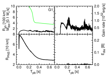
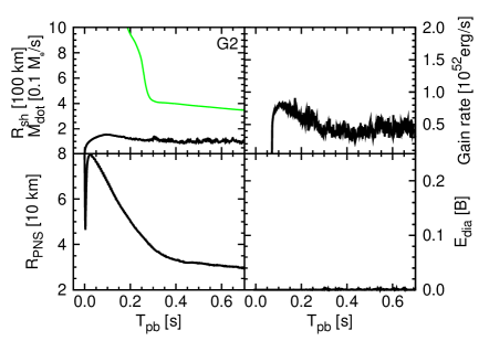
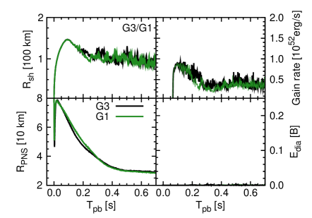
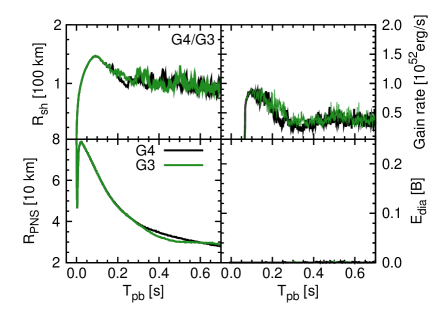
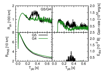
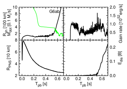
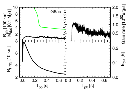
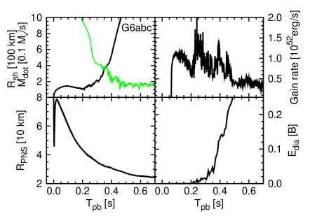
Figure 17: Summary of our 2D models (see text).

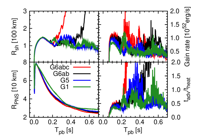
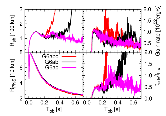
Figure 18: Same as Figure 17 but for the comparison between the 2D exploding and non-exploding models (top panel) and the comparison between models G6ab, G6ac, and G6abc (bottom panel). Note that the bottom right panel shows ”$t_{\rm adv}/t_{\rm heat}$” which denotes the ratio of advection to heating timescale in the gain region (Buras et al., 2006b).

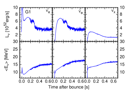
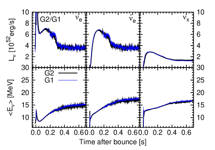
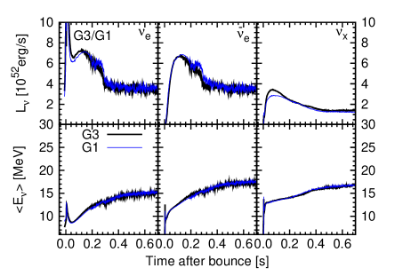
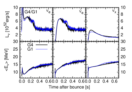
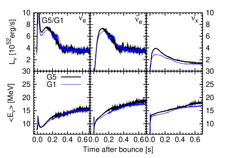
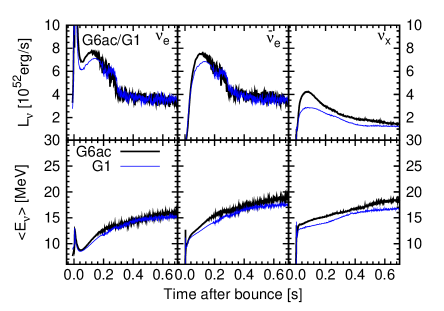
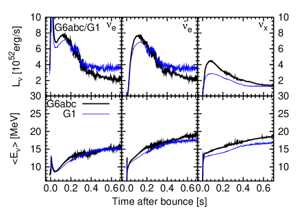
Figure 19: Comparison of neutrino luminosities (upper panels) and the rms neutrino energies (lower panels) for all the 2D models.

Three panels in the second and third raw of Figure 17 show more detailed comparison between G3 and G1 (labeled with G3/G1), G4 and G3 (with G4/G3), G5 and G4 (with G5/G4), respectively. Regarding the shock evolution (second raws), the average shock radii of G3 and G4 (black lines) show no remarkable difference from G1 (green line). This is in line with the lack of significant change in the net heating rate (top right) relative to G1. As expected in 1D, the inclusion of the nupair reaction (Section 3.3) makes the PNS radius more compact compared to G1 (see panel labeled with G3/G1). The PNS radius of G4 somehow becomes slightly bigger between $\sim$ 375 - 600 ms compared to G3, however comes closer to G3 thereafter. From Figure 19, the neutrino luminosities and rms energies show no clear discrepancies between G3 and G4 compared to those already observed in the corresponding 1D models.

More big change can be seen in the shock evolution of G5 (black line, see panel with G5/G4 in Figure 17). The shock of G5 (black line) starts to expand at $\sim 214$ ms after bounce (see the hump in the shock evolution), maximally reaching at $\sim 163$ km, but returns to closely match with the shock trajectory of G4 (green line) after 400 ms postbounce (see also Figure 16). In fact, the rms energies of $\nu_{e}$ and $\bar{\nu}_{e}$ are higher for G5 than G1 (see the panel with G5/G1 in Figure 19) and the net heating rate (top panel of Figure 18) becomes clearly larger for G5 (blue line) compared to G1 (green line) during the transient shock expansion phase. This is reconciled with the (slightly) higher heating rate due to the weak magnetism and recoil effect (as we saw in our 1D model, set5a). The higher heating rate is also fingerprinted in the diagnostic explosion energy (black line, see the panel with G5/G4 in Figure 17).

Using the same progenitor, LS220 EOS, and the similar set of neutrino opacities, our G5 run is close to model s20-2007 of Summa et al. (2016). Their s20-2007 start to explode $\sim 200-300$ ms after bounce, whereas our G5 does not. For a quantitative discussion, we choose to compare the neutrino luminosities and the rms energies at 100 ms after bounce, which closely corresponds to the peak of the luminosities (e.g., their Figure 3). For the progenitor, the luminosity of $\nu_{e}$, $\bar{\nu}_{e}$, and $\nu_{x}$ is $\sim$7.0, 6.5, and 4.2 $\times 10^{52}$erg/s for s20-2007, and $7.5$, $7.5$, and $4.0$ times $\times 10^{52}$erg/s for G5, respectively. The rms energy of $\nu_{e}$, $\bar{\nu}_{e}$, and $\nu_{x}$ is $\sim$12.2, 14.4, and 16.2 MeV for s20-2007, and $11.0$, $13.8$, and $14.9$ $\times 10^{52}$erg/s for G5, respectively. The lower $\nu_{e}$ and $\bar{\nu}_{e}$ rms energies would explain more difficult explosion for G5 compared to s20-2007 of Summa et al. (2016). As already mentioned, our neglect of the non-elastic effects in the charged current reactions, the simplified transport schemes could explain such $\sim 10\%$ level of discrepancies. We cannot unambiguously identify which of the missing sophistication in this work could explain the above difference. This apparently manifests that implementation of detailed neutrino opacities and accurate treatment of neutrino transport as well as GR are mandatory for quantitative studies of the CCSN mechanism.

G6ab shows a shock revival at $\sim 500$ ms after bounce (Figure 16), which we can see also from the clear deviation of the diagnostic energy from zero (see the panel labeled by G6ab in Figure 17). On the other hand, G6ac is not exploding during the simulation time (Figure 16). The neutrino luminosities and rms energies show fast time variations in the accretion phase (Figure 19), it is not easy to clearly see the increase for G6ab relative to G5.

In order to understand the above trend, we show the ratio of advection to heating timescale in the gain region (Buras et al., 2006b) (the bottom panel in Figure 18 (bottom right)). From the panel, one can see that the strangeness contribution (magenta line, G6ac) does enhance the chance of explosion at around 300 ms postbounce, which can be seen as peaks of the ratio (”$t_{\rm adv}$/$t_{\rm heat}$”) exceeding unity. In fact, the shock radius (the top left panel) and the net heating rate in the gain region (the top right panel) becomes slightly bigger for G6ac (magenta lines) comparing to those of G6ab (black lines) at the same time.

The enhanced chance of explosion in models with the strangeness correction (G6ac and G6abc) originates from the reduction of the neutrino opacity, which is most significant in the accretion phase. This was already seen in our 1D runs of the $15M_{\odot}$ star (see the green line in the right panel of Figure 14 in the accretion phase). Our 2D results show that the inclusion of only the strangeness correction (relative to the standard rates) is not sufficient to trigger the onset of explosion for the 20 $M_{\odot}$ star. As one can see from the red line (G6abc, the bottom panel in Figure 18), our 2D run demonstrates that the combination of the strangeness and the many-body correction makes the onset of the explosion easier.

As already mentioned in our 1D comparison (Section 3.6), the many-body correction of Horowitz et al. (2017) is expected to enhance the explodability primarily after the accretion phase because the many-body corretion reduces the opacity at high densities. Our 2D results are in line with the 1D expectation. The net heating rate in the gain region is higher and the PNS radius is slightly smaller for G6ab comparing to those of G5 (and G1) in the post accretion phase (e.g., top panel of Figure 18). These results demonstrate that the many-body correction mainly impacts the explodability also in 2D after the accretion phase. Using the same EOS (LS220) and the same progenitor, model s20.0-LS220 in Bollig et al. (2017) that includes the many-body correction in addition to their standard neutrino opacities leads to explosion after $\sim$ 400 ms postbounce (see, sky-blue line in the top right panel of their Figure 1), whereas the corresponding model further including the strangeness correction ($g^{s}_{a}=-0.1$) leads to more earlier explosion at $\sim$ 200 ms postbounce (e.g., blue line in their Figure 1). These features are basically consistent with our 2D runs.

Finally, G6abc (Figure 16) shows the earliest runaway shock expansion (starting at $\sim 200$ ms after bounce) among our 2D models. As already seen in set6c (Section 3.6), the strangeness effects contribute to enhance the $\nu_{e}$ and $\bar{\nu}_{e}$ luminosity before the accretion phase ends ($\sim 300$ ms after bounce). Quantitatively, the peak of the accretion luminosity of $\nu_{e}$ and $\bar{\nu}_{e}$ is enhanced by $\sim 3.8\%$ and $\sim 1.3\%$ for G6abc compared to G6ab (e.g., Figure 19). The slightly enhanced heating rate in the accretion phase due to the strangeness correction works synergetically with the many-body correction to revive the stalled shock into explosion for the 20 $M_{\odot}$ star (e.g., Figure 18). The diagnostic energy when the shock reaches at 1000 km is 0.24 B and 0.2 B with B representing ”Bethe” = $10^{51}$ erg. To get the saturated value, long-term simulations are needed, which is beyond the scope of this work. Using the same progenitor and the LS220 EOS, the onset time of an explosion ($\sim 200$ ms after bounce) is close to that seen in the 2D model of Bollig et al. (2017) with the strangeness contribution ($g^{s}_{a}=-0.1$). However, the match may be simply incidental because the contributions from muons are not yet included in this work.

5 Conclusions and Discussion

In this study, we have explored impact of updated neutrino opacities in CCSN simulations where spectral neutrino transport is solved by the three-flavor IDSA scheme. To verify our code, we first presented 1D results following core-collapse, bounce, and up to $\sim 250$ ms postbounce of a $15M_{\odot}$ star using the standard set of neutrino opacities by Bruenn (1985) and made a comparison with the seminal work by Liebendörfer et al. (2005). A good agreement of the code comparison supports the reliability of our three-flavor IDSA scheme with the standard opacity set. Then we investigated in 1D runs how the individual updated rate could lead to the difference from the base-line run with the standard opacity set. By making a detailed comparison with previous literature, we have checked the validity of our each implementation in a step-by-step manner. As previously identified, we have confirmed that adding up the individual rates impacts non-linearly the neutrino luminosities and energies. In our 2D runs, we implemented selected sets of the neutrino opacities because a full investigation of the individual rates is currently too computationally expensive to do even in 2D with our improved IDSA scheme. Regarding the explodability, our results showed that several expectations from the individual update in 1D are indeed correct in 2D. Among the updates considered in this work, the inclusion of both the strangeness-dependent contribution and the many-body correction to the neutrino-nucleon scattering has the largest impact in enhancing the explodability in our 2D models.

Using the same progenitor, the same EOS, and the similar set of the neutrino opacities, there are $\sim 10\%$ levels of discrepancies in the neutrino luminosities and the rms energies between our results and the results from the codes with more accurate neutrino transport schemes (e.g., Agile-BOLTZTRAN and Vertex). Our neglect of energy-bin/flavor coupling in the transport equation, non-isoenergetic effects in the charged current reactions, and the partial implementation of the Doppler-shift terms could solve the mismatch. Moreover, our approximate GR treatment as well as in the neutrino transport should be also improved. In this respect, the microphysical update we have done in this work is nothing but among the first steps toward more sophisticated CCSN modeling.

Appendix A Implementing electron neutrino pair annihilation

A.1 $\nu_{e}+\bar{\nu}_{e}\rightarrow\nu_{x}+\bar{\nu}_{x}$: evolution equation of $\nu_{x}$

Following Buras et al. (2003), the scattering kernels of the electron-neutrino pair-annihilation can be calculated essentially in the same way as electron-positron annihilation, $e^{-}+e^{+}\rightarrow\nu_{x}+\bar{\nu}_{x}$. It is convenient to define the $\nu_{x}$ pair-production kernels labelled (p),

$$\mathcal{R}_{\nu_{x}\bar{\nu}_{x}}^{\rm p}(\cos\theta_{\nu_{x}\bar{\nu}_{x}},E_{\nu_{x}}+E_{\bar{\nu}_{x}})=\int\frac{d^{3}p_{\nu_{e}}}{(2\pi\hbar)^{3}}\frac{d^{3}p_{\bar{\nu}_{e}}}{(2\pi\hbar)^{3}}2f_{\nu_{e}}(p_{\nu_{e}})2f_{\bar{\nu}_{e}}(p_{\bar{\nu}_{e}})\left|\mathcal{M}\right|^{2}\delta^{4}(p_{\nu_{e}}+p_{\bar{\nu}_{e}}-p_{\nu_{x}}-p_{\bar{\nu}_{x}})~{},$$ (A1)

with the initial-particle’s distribution functions $f_{\nu_{e}}$ and $f_{\bar{\nu}_{e}}$, for which we assume local thermodynamic equilibrium, i.e. $\mu_{\nu_{e}}=\mu_{e}-(\mu_{n}-\mu_{p})$. The pair-production kernel (B1) depends on the incident scattering angle $\theta_{\nu_{x}\bar{\nu}_{x}}$ between $\nu_{x}$ and $\bar{\nu}_{x}$ (for the definition, cf., Mezzacappa & Bruenn, 1993b) as well as on the sum of $\nu_{x}$ and $\bar{\nu}_{x}$ energies, $E_{\nu_{x}}$ and $E_{\bar{\nu}_{x}}$ respectively. Moreover, the spin-averaged and squared matrix element, $\left|\mathcal{M}\right|^{2}$, is obtained from $e^{-}-e^{+}$-annihilation (cf. Bruenn, 1985) with the following replacements for the weak coupling constants, $C_{V}=C_{A}=+1/2$. Since within the IDSA no explicit angle-dependence of weak processes is employed, we perform a Legendre expansion of the pair-production kernel (B1) in terms of $\cos\theta$,

$$\mathcal{R}_{\nu\bar{\nu}}^{\rm p}(\cos\theta_{\nu\bar{\nu}},E_{\nu}+E_{\bar{\nu}})\longrightarrow\frac{1}{2}\Phi_{0,\nu\bar{\nu}}^{\rm p}(E_{\nu}+E_{\bar{\nu}})+\mathcal{O}(\cos\theta)~{},$$ (A2)

such that the corresponding collision term for the the zeroth component of the distribution function, $f_{\nu_{x}}^{(0)}$, reads as follows,

$$\left.\frac{\partial f_{\nu_{x}}^{(0)}(E_{\nu_{x}})}{c\partial t}\right|_{\rm coll} = \frac{2\pi}{c(2\pi\hbar c)^{3}}\left(1-f_{\nu_{x}}^{(0)}(E_{\nu_{x}})\right)\int E_{\bar{\nu}_{x}}^{2}dE_{\bar{\nu}_{x}}\left(1-f_{\bar{\nu}_{x}}^{(0)}(E_{\bar{\nu}_{x}})\right)\Phi_{0,\nu_{x}\bar{\nu}_{x}}^{\rm p}(E_{\nu_{x}}+E_{\bar{\nu}_{x}})$$ (A3)

$$- \frac{2\pi}{c(2\pi\hbar c)^{3}}f_{\nu_{x}}^{(0)}(E_{\nu_{x}})\int E_{\bar{\nu}_{x}}^{2}dE_{\bar{\nu}_{x}}f_{\bar{\nu}_{x}}^{(0)}(E_{\bar{\nu}_{x}})\Phi_{0,\nu_{x}\bar{\nu}_{x}}^{\rm a}(E_{\nu_{x}}+E_{\bar{\nu}_{x}})~{},$$

where $\Phi_{0,\nu_{x}\bar{\nu}_{x}}^{\rm a}$ denotes the zeroth-order Legendre coefficient of the $\nu_{x}$-pair absorption kernel. It is related to $\Phi_{0,\nu_{x}\bar{\nu}_{x}}^{\rm p}$ via the relation of detailed balance,

$$\Phi_{0,\nu_{x}\bar{\nu}_{x}}^{\rm a}(E_{\nu_{x}}+E_{\bar{\nu}_{x}})=\exp\left\{\frac{E_{\nu_{x}}+E_{\bar{\nu}_{x}}}{T}\right\}\Phi_{0,\nu_{x}\bar{\nu}_{x}}^{\rm p}(E_{\nu_{x}}+E_{\bar{\nu}_{x}})~{},$$ (A4)

which is realized straight forward in a similar fashion as expression (B1). Now, Eq. (A3) can be rewritten as follows,

$$\left.\frac{\partial f_{\nu_{x}}^{(0)}(E_{\nu_{x}})}{c\partial t}\right|_{\rm coll}=C^{0}_{\rm nupair}(E_{\nu_{x}})+A^{0}_{\rm nupair}(E_{\nu_{x}})\,f_{\nu_{x}}^{(0)}(E_{\nu_{x}})~{},$$ (A5)

with

$$C^{0}_{\rm nupair}(E_{\nu_{x}}) = \frac{2\pi}{c(2\pi\hbar c)^{3}}\int E_{\bar{\nu}_{x}}^{2}dE_{\bar{\nu}_{x}}\left(1-f_{\bar{\nu}_{x}}^{(0)}(E_{\bar{\nu}_{x}})\right)\Phi_{0,\nu_{x}\bar{\nu}_{x}}^{\rm p}(E_{\nu_{x}}+E_{\bar{\nu}_{x}})~{},$$ (A6)

$$A^{0}_{\rm nupair}(E_{\nu_{x}}) = -\frac{2\pi}{c(2\pi\hbar c)^{3}}\int E_{\bar{\nu}_{x}}^{2}dE_{\bar{\nu}_{x}}\left[\left(1-f_{\bar{\nu}_{x}}^{(0)}(E_{\bar{\nu}_{x}})\right)\Phi_{0,\nu_{x}\bar{\nu}_{x}}^{\rm p}(E_{\nu_{x}}+E_{\bar{\nu}_{x}})\right.$$ (A7)

$$\;\,+\left.f_{\bar{\nu}_{x}}^{(0)}(E_{\bar{\nu}_{x}})\Phi_{0,\nu_{x}\bar{\nu}_{x}}^{\rm a}(E_{\nu_{x}}+E_{\bar{\nu}_{x}})\right]~{},$$

which denote the production Eq. (A6) and annihilation rates Eq. (A7) of this process, respectively. In the IDSA, the terms $C^{0}_{\rm nupair}$ and $A^{0}_{\rm nupair}$ are added to the Eqs. (5) and (6) for the streaming neutrinos and to Eq. (15) of Liebendörfer et al. (2009) for the trapped neutrinos.

A.2 $\nu_{e}+\bar{\nu}_{e}\rightarrow\nu_{x}+\bar{\nu}_{x}$: evolution equations of $\nu_{e}$ and $\bar{\nu}_{e}$

The collision term for $f_{\nu_{e}}^{0}$ associated with this process is obtained in a similar fashion as for the production of $\nu_{x}$-pairs A.1,

$$\left.\frac{\partial f_{\nu_{e}}^{(0)}(E_{\nu_{e}})}{c\partial t}\right|_{\rm coll} = \frac{2\pi}{c(2\pi\hbar c)^{3}}\left(1-f_{\nu_{e}}^{(0)}(E_{\nu_{e}})\right)\int E_{\bar{\nu}_{e}}^{2}dE_{\bar{\nu}_{e}}\left(1-f_{\bar{\nu}_{e}}^{(0)}(E_{\bar{\nu}_{e}})\right)\Phi_{0,\nu_{e}\bar{\nu}_{e}}^{\rm p}(E_{\nu_{e}}+E_{\bar{\nu}_{e}})$$ (A8)

$$- \frac{2\pi}{c(2\pi\hbar c)^{3}}f_{\nu_{e}}^{(0)}(E_{\nu_{e}})\int E_{\bar{\nu}_{e}}^{2}dE_{\bar{\nu}_{e}}f_{\bar{\nu}_{e}}^{(0)}(E_{\bar{\nu}_{e}})\Phi_{0,\nu_{e}\bar{\nu}_{e}}^{\rm a}(E_{\nu_{e}}+E_{\bar{\nu}_{e}})~{}.$$

Note that the expression for the collision integral for $\bar{\nu}_{e}$ is obtained equivalently by replacing the labels $\nu_{e}\leftrightarrow\bar{\nu}_{e}$ in above expression. Moreover, due to the following symmetry considerations,

$$\Phi_{0,\nu_{e}\bar{\nu}_{e}}^{\rm p}=\Phi_{0,\nu_{x}\bar{\nu}_{x}}^{\rm a}~{},\;\;\;\;\;\Phi_{0,\nu_{e}\bar{\nu}_{e}}^{\rm a}=\Phi_{0,\nu_{x}\bar{\nu}_{x}}^{\rm p}~{},$$ (A9)

expression (A8) can be reduced to a similarly simple form as expression (A5), with equivalent definitions for $C^{0}$ and $A^{0}$. Due to the relation of detailed balance (B3), which holds here as well, it becomes clear that it is necessary to obtain only one pair-reaction kernel, e.g., $\phi_{0,\nu_{x}\bar{\nu}_{x}}^{\rm p}$. Therefore, we follow Eq. (C62)–(C74) in Bruenn (1985) for the computation presented in this work. Note that also here we assume that $\nu_{x}$ obey local thermodynamic equilibrium, i.e. $\mu_{\nu_{x}}=0$ (this was also assumed in Buras et al., 2003; Fischer et al., 2009). For practical reasons we monitor the $\nu_{e}$-distribution function which must not differ by more than 10% from the corresponding Fermi-Dirac distribution. This treatment was tested to work well in Agile-BOLTZTRAN simulations by Fischer et al. (2009).

A.3 Integrated pair production rates

Here we provide definitions of quantities shown in the main part of the present paper. Therefore, the $(\nu_{x},\bar{\nu}_{x})$ pair production rate is defined as follows,

$$Q_{\nu_{x}\bar{\nu}_{x}}(E_{\nu_{x}}) = \frac{1}{(2\pi\hbar c)^{3}}\int E_{\bar{\nu}_{x}}^{2}dE_{\bar{\nu}_{x}}\left(1-f_{\bar{\nu}_{x}}^{(0)}(E_{\bar{\nu}_{x}})\right)2\pi\Phi_{0,\nu_{x}\bar{\nu}_{x}}^{\rm p}(E_{\nu_{x}}+E_{\bar{\nu}_{x}})\;\;\;\;\;\;[{\rm s}^{-1}]~{},$$ (A10)

such that the total number production rate of $\nu_{x}$ is given as follows,

$$\frac{\partial n_{\nu_{x}}}{\partial t} = \frac{1}{(2\pi\hbar c)^{3}}\frac{1}{n_{\nu_{x}}}\int E_{\nu_{x}}^{2}dE_{\nu_{x}}\left(1-f_{\nu_{x}}^{(0)}(E_{\nu_{x}})\right){4\pi}Q_{\nu_{x}\bar{\nu}_{x}}(E_{\nu_{x}})~{},$$ (A11)

normalized to the number density of neutrinos $n_{\nu_{x}}$. Then, we obtain the number production spectra,

$$\frac{\partial^{2}n_{\nu_{x}}}{\partial E_{\nu_{x}}\partial t} = \frac{1}{(2\pi\hbar c)^{3}}E_{\nu_{x}}^{2}\left(1-f_{\nu_{x}}^{(0)}(E_{\nu_{x}})\right)4\pi Q_{\nu_{x}\bar{\nu}_{x}}(E_{\nu_{x}})\;\;\;\;\;\;[{\rm s}^{-1}~{}{\rm MeV}^{-1}~{}{\rm cm}^{-3}]~{},$$ (A12)

which is shown in the left panel of Fig. 6 for some selected conditions, and the energy production spectra,

$$\frac{\partial^{2}\varepsilon_{\nu_{x}}}{\partial E_{\nu_{x}}\partial t} = \frac{1}{(2\pi\hbar c)^{3}}E_{\nu_{x}}^{3}\left(1-f_{\nu_{x}}^{(0)}(E_{\nu_{x}})\right)4\pi Q_{\nu_{x}\bar{\nu}_{x}}(E_{\nu_{x}})\;\,\;\;\;\;[{\rm s}^{-1}~{}{\rm cm}^{-3}]~{},$$ (A13)

which is shown in the right panel of Fig. 6.

Appendix B $\nu_{x}+\nu_{e}(\bar{\nu}_{e})\leftrightarrows\nu^{\prime}_{e}(\bar{\nu}^{\prime}_{e})+\nu^{\prime}_{x}$

For the calculation of the scattering kernel we follow the same procedure as for neutrino-electron(positron) scattering (Buras et al., 2003),

$$\mathcal{R}_{\nu_{x}}^{\rm in}(\cos\theta_{\nu_{x}\nu^{\prime}_{x}},E_{\nu_{x}}-E_{\nu^{\prime}_{x}})=\int\frac{d^{3}p_{\nu_{e}}}{(2\pi\hbar)^{3}}\frac{d^{3}p_{\nu^{\prime}_{e}}}{(2\pi\hbar)^{3}}2f_{\nu^{\prime}_{e}}(p_{\nu^{\prime}_{e}})\left(1-f_{\nu_{e}}(p_{\nu_{e}})\right)\left|\mathcal{M}\right|^{2}\delta^{4}(p_{\nu_{x}}+p_{\nu_{e}}-p_{\nu^{\prime}_{x}}-p_{\nu^{\prime}_{x}})~{},$$ (B1)

which is evaluated under the assumption of local thermodynamic equilibrium, exactly as for the neutrino-pair processes in appendix A. Here the spin-averaged and squared matrix element, $\left|\mathcal{M}\right|^{2}$, is obtained from neutrino-electron scattering (cf. Bruenn, 1985) with the following replacements for the weak coupling constants, $C_{V}=C_{A}=+1/2$ for $\nu_{x}$-scattering on $\nu_{e}$ and $C_{V}-1$ and $C_{A}-1$ for $\nu_{x}$-scattering on $\bar{\nu}_{e}$. With the Legendre expansion of the scattering kernel in terms of $\cos\theta_{\nu\nu^{\prime}}$, we obtain the zeroth-order term of the collision integral for $f_{\nu_{x}}^{0}$ as follows,

$$\frac{\partial f_{\nu_{x}}^{(0)}(E_{\nu_{x}})}{\partial t}\Big{|}_{\rm coll} = \frac{2\pi}{c(2\pi\hbar c)^{3}}\left(1-f_{\nu_{x}}^{(0)}(E_{\nu_{x}})\right)\int E_{\nu^{\prime}_{x}}^{2}dE_{\nu^{\prime}_{x}}f_{\nu^{\prime}_{x}}^{(0)}(E_{\nu^{\prime}_{x}})\Phi_{0,\nu_{x}}^{\rm in}(E_{\nu_{x}}-E_{\nu^{\prime}_{x}})$$ (B2)

$$- \frac{2\pi}{c(2\pi\hbar c)^{3}}f_{\nu_{x}}^{(0)}(E_{\nu_{x}})\int E_{\nu^{\prime}_{x}}^{2}dE_{\nu^{\prime}_{x}}(1-f_{\nu^{\prime}_{x}}^{(0)})(E_{\nu^{\prime}_{x}})\Phi_{0,\nu_{x}}^{\rm out}(E_{\nu_{x}}-E_{\nu^{\prime}_{x}})~{},$$

where the out-scattering kernel, $\Phi_{0,\nu_{x}}^{\rm out}$, is obtained via the relation of detailed balance,

$$\Phi_{0,\nu_{x}}^{\rm out}(E_{\nu_{x}}-E_{\nu^{\prime}_{x}})=\exp\left\{\frac{E_{\nu_{x}}-E_{\nu^{\prime}_{x}}}{T}\right\}\Phi_{0,\nu_{x}}^{\rm in}(E_{\nu_{x}}-E_{\nu^{\prime}_{x}})~{}.$$ (B3)

Similarly as Equations (A6) and (A7), one can obtain $C^{0}_{\rm NNS}$ and $A^{0}_{\rm NNS}$ for the neutrino-neutrino scattering (NNS) processes here. These are added to the evolution equation of the streaming and trapped neutrinos, accordingly. Note that the expression for $\nu_{x}$-scattering on $\bar{\nu}_{e}$ is obtained equivalently by replacing the labels $\nu_{e}\leftrightarrow\bar{\nu}_{e}$ in the above expressions. For the calculations of the scattering kernels, we follow Eq. (C50) in Bruenn (1985) for the computation presented in this work. Then, the inverse mean-free path $1/\lambda_{\rm mfp}$ shown in Fig. 8 is obtained as follows,

$$A_{\rm NNS,\nu_{x}}^{0}(E_{\nu_{x}}) = -\frac{2\pi}{c(2\pi\hbar c)^{3}}\int E_{\nu_{x}^{\prime}}^{2}dE_{\nu_{x}^{\prime}}\left(f_{\nu_{x}^{\prime}}^{(0)}(E_{\nu_{x}^{\prime}})\Phi_{0,\nu_{x}}^{\rm in}(E_{\nu_{x}}-E_{\nu_{x}^{\prime}})\right.$$ (B4)

$$\left.+\left(1-f_{\nu_{x}^{\prime}}^{(0)}(E_{\nu_{x}^{\prime}})\right)\Phi_{0,\nu_{x}}^{\rm out}(E_{\nu_{x}}-E_{\nu_{x}^{\prime}})\right)$$

where $1/\lambda_{\rm mfp}=A_{\rm NNS,\nu_{x}}^{0}$ in units of [s^-1], which holds also for the other processes (cf., Equation (139) of Kuroda et al., 2016).

References

- Abdikamalov et al. (2016) Abdikamalov, E., Zhaksylykov, A., Radice, D., & Berdibek, S. 2016, MNRAS, 461, 3864
- Antoniadis et al. (2013) Antoniadis, J., Freire, P. C. C., Wex, N., Tauris, T. M., Lynch, R. S., van Kerkwijk, M. H., Kramer, M., Bassa, C., Dhillon, V. S., Driebe, T., Hessels, J. W. T., Kaspi, V. M., Kondratiev, V. I., Langer, N., Marsh, T. R., McLaughlin, M. A., Pennucci, T. T., Ransom, S. M., Stairs, I. H., van Leeuwen, J., Verbiest, J. P. W., & Whelan, D. G. 2013, Science, 340, 448
- Bartl et al. (2016) Bartl, A., Bollig, R., Janka, H.-T., & Schwenk, A. 2016, Phys. Rev. D, 94, 083009
- Bethe & Wilson (1985) Bethe, H. A. & Wilson, J. R. 1985, ApJ, 295, 14
- Blondin et al. (2003) Blondin, J. M., Mezzacappa, A., & DeMarino, C. 2003, ApJ, 584, 971
- Bollig et al. (2017) Bollig, R., Janka, H.-T., Lohs, A., Martínez-Pinedo, G., Horowitz, C. J., & Melson, T. 2017, Physical Review Letters, 119, 242702
- Bruenn (1985) Bruenn, S. W. 1985, ApJS, 58, 771
- Bruenn et al. (2013) Bruenn, S. W., Mezzacappa, A., Hix, W. R., Lentz, E. J., Bronson Messer, O. E., Lingerfelt, E. J., Blondin, J. M., Endeve, E., Marronetti, P., & Yakunin, K. N. 2013, ApJ, 767, L6
- Buras et al. (2003) Buras, R., Janka, H.-T., Keil, M. T., Raffelt, G. G., & Rampp, M. 2003, ApJ, 587, 320
- Buras et al. (2006a) Buras, R., Janka, H.-T., Rampp, M., & Kifonidis, K. 2006a, A&A, 457, 281
- Buras et al. (2006b) Buras, R., Rampp, M., Janka, H.-T., & Kifonidis, K. 2006b, A&A, 447, 1049
- Burrows (2013) Burrows, A. 2013, Reviews of Modern Physics, 85, 245
- Burrows & Sawyer (1998) Burrows, A. & Sawyer, R. F. 1998, Phys. Rev. C, 58, 554
- Burrows & Sawyer (1999) —. 1999, Phys. Rev. C, 59, 510
- Burrows et al. (2016) Burrows, A., Vartanyan, D., Dolence, J. C., Skinner, M. A., & Radice, D. 2016, ArXiv e-prints
- Carter & Prakash (2002) Carter, G. W. & Prakash, M. 2002, Physics Letters B, 525, 249
- Colgate & White (1966) Colgate, S. A. & White, R. H. 1966, ApJ, 143, 626
- Couch et al. (2015) Couch, S. M., Chatzopoulos, E., Arnett, W. D., & Timmes, F. X. 2015, ApJ, 808, L21
- Couch & Ott (2013) Couch, S. M. & Ott, C. D. 2013, ApJ, 778, L7
- Demorest et al. (2010) Demorest, P. B., Pennucci, T., Ransom, S. M., Roberts, M. S. E., & Hessels, J. W. T. 2010, Nature, 467, 1081
- Dolence et al. (2014) Dolence, J. C., Burrows, A., & Zhang, W. 2014, ArXiv e-prints
- Einfeldt (1988) Einfeldt, B. 1988, SIAM Journal on Numerical Analysis, 25, 294
- Endeve et al. (2012) Endeve, E., Cardall, C. Y., Budiardja, R. D., Beck, S. W., Bejnood, A., Toedte, R. J., Mezzacappa, A., & Blondin, J. M. 2012, ApJ, 751, 26
- Fischer (2016) Fischer, T. 2016, A&A, 593, A103
- Fischer et al. (2014) Fischer, T., Hempel, M., Sagert, I., Suwa, Y., & Schaffner-Bielich, J. 2014, European Physical Journal A, 50, 46
- Fischer et al. (2013) Fischer, T., Langanke, K., & Martínez-Pinedo, G. 2013, Phys. Rev. C, 88, 065804
- Fischer et al. (2012) Fischer, T., Martínez-Pinedo, G., Hempel, M., & Liebendörfer, M. 2012, Phys. Rev. D, 85, 083003
- Fischer et al. (2009) Fischer, T., Whitehouse, S. C., Mezzacappa, A., Thielemann, F.-K., & Liebendörfer, M. 2009, A&A, 499, 1
- Foglizzo et al. (2015) Foglizzo, T., Kazeroni, R., Guilet, J., Masset, F., González, M., Krueger, B. K., Novak, J., Oertel, M., Margueron, J., Faure, J., Martin, N., Blottiau, P., Peres, B., & Durand, G. 2015, Publications of the Astronomical Society of Australiam, 32, e009
- Fuller et al. (1982) Fuller, G. M., Fowler, W. A., & Newman, M. J. 1982, ApJS, 48, 279
- Guilet & Müller (2015) Guilet, J. & Müller, E. 2015, MNRAS, 450, 2153
- Hanke et al. (2013) Hanke, F., Müller, B., Wongwathanarat, A., Marek, A., & Janka, H.-T. 2013, ApJ, 770, 66