Revealed Price Preference: Theory and Empirical Analysis

Abstract.

To determine the welfare implications of price changes in demand data, we introduce a revealed preference relation over prices. We show that the absence of cycles in this relation characterizes a consumer who trades off the utility of consumption against the disutility of expenditure. Our model can be applied whenever a consumer’s demand over a strict subset of all available goods is being analyzed; it can also be extended to settings with discrete goods and nonlinear prices. To illustrate its use, we apply our model to a single-agent data set and to a data set with repeated cross-sections. We develop a novel test of linear hypotheses on partially identified parameters to estimate the proportion of the population who are revealed better off due to a price change in the latter application. This new technique can be used for nonparametric counterfactual analysis more broadly.

1. Introduction

A central question in economic analysis is the determination of the welfare effect of price changes. As an example, suppose we observe a consumer’s purchases of two goods, gasoline and food, from two separate trips to a grocery store with an on site gasoline retailer. In the first instance $t$, the prices are $p^{t}=(2,2)$ of gasoline and food respectively and she buys a bundle $x^{t}=(6,3)$. In her second trip $t^{\prime}$, the prices are $p^{t^{\prime}}=(3,1)$ and she purchases $x^{t^{\prime}}=(5,4)$. The most basic welfare question one can ask here is whether the consumer is better off at the prices prevailing at $t$ or at $t^{\prime}$ (keeping fixed the prices of all other goods she consumes)? In this paper, we introduce a theoretical framework based on revealed preference, along with a nonparametric econometric technique, that would allow us to answer questions of this type.

A typical approach to this problem is to model the consumer as having a quasilinear utility function $\widetilde{U}(x)-p\cdot x$ since, in particular, this allows for simple “sufficient statistics” analysis of welfare gains or losses using a Harberger formula (see Chetty (2009) and most recently Kleven (2021) for an overview of this approach). Of course, the second term ($-p\cdot x$) in the quasilinear utility function captures the fact that the goods being analyzed (food and gasoline in our simple example) do not constitute the universe of the consumer’s consumption; expenditure lowers utility because it reduces the consumption of an outside (numeraire) good.

The point of departure of our analysis is the following simple observation. Without having to model the consumer’s preference as quasilinear (or taking any other specific functional form) we can still conclude that she is better off at $t$ compared to $t^{\prime}$. This is because $p^{t^{\prime}}\cdot x^{t^{\prime}}=19$ whereas $p^{t}\cdot x^{t^{\prime}}=18$. In other words, if the prices prevailing at $t^{\prime}$ were $p^{t}$ instead of $p^{t^{\prime}}$, the consumer would be better off since purchasing the same bundle $x^{t^{\prime}}$ would cost less, leaving the consumer with more money to buy other goods (outside the set of goods analyzed). More generally, the consumer has a preference over prices that an analyst could at least partially discern from the data: if at observations $t$ and $t^{\prime}$, we find that $p^{t}\cdot x^{t^{\prime}}\leq(<)p^{t^{\prime}}\cdot x^{t^{\prime}}$, then

the consumer has revealed that she (strictly) prefers the price $p^{t}$ to the price $p^{t^{\prime}}$.

Welfare comparisons made in this way will only be consistent if the revealed preference relation over prices is free of cycles, a property we call the generalized axiom of price preference (GAPP). This leads inevitably to the following question: precisely what does GAPP mean for consumer behavior?

Augmented Utility Functions:  To answer this question, we assume that the analyst collects a data set $\mathcal{D}=\{p^{t},x^{t}\}_{t=1}^{T}$ from a consumer; each observation $t$ consists of the prices $p^{t}\in\mathbb{R}^{L}_{++}$ of $L$ goods (representing some but not all the goods she consumes) and the consumer’s demand $x^{t}\in\mathbb{R}^{L}_{+}$ at those prices. We show that GAPP (on $\mathcal{D}$) is both necessary and sufficient for the existence of a strictly increasing function $U:\mathbb{R}^{L}_{+}\times\mathbb{R}_{-}\to\mathbb{R}$ that rationalizes $\mathcal{D}$ in the following sense:

$$x^{t}\in\operatornamewithlimits{argmax}_{x\in\mathbb{R}^{L}_{+}}U(x,-p^{t}\cdot x)\>\mbox{ for all $t=1,2,...,T$.}$$

The function $U$ should be interpreted as an expenditure-augmented utility function, where $U(x,-e)$ is the consumer’s utility when she acquires $x$ at the cost of $e$. It recognizes that the consumer’s expenditure on the observed goods is endogenous and dependent on prices: she could in principle spend more than what she actually spent (note that she optimizes over $x\in\mathbb{R}^{L}_{+}$) but the trade-off is the dis-utility of greater expenditure. Note that the quasilinear utility function $U(x,-p\cdot x)=\widetilde{U}(x)-p\cdot x$ is a special case of an augmented utility function.

The augmented utility model has a number of features that makes it widely applicable and easy to use. We highlight a few of them.

(1)  Being more general than the quasilinear model, it does not have some of its overly strong implications on the structure of consumer demand (see Section 2.3). In particular, it is broad enough to accommodate phenomena emphasized in the behavioral economics literature, such as reference dependence, mental budgeting and inattention to prices. We briefly describe the first of these here, a more detailed discussion can be found in Section 2.4. Kőszegi and Rabin (2006) and Heidhues and Kőszegi (2008) argue that consumption decisions can depend not just on the actual prices but also on the prices the consumer expected to pay. Specifically, the disutility from spending is greater if the expected price was lower than the sticker price and vice versa. A simple way they propose of capturing this phenomenon is the following function

$$U(x,-px)=\widetilde{U}(x)-p\cdot x-F(p\cdot x-\tilde{p}\cdot x).$$

The first two terms capture standard quasilinear preferences whereas the third term captures a general form of reference dependence. In Koszegi and Rabin’s terminology, the consumer gets “gain-loss utility” by comparing the expenditure $p\cdot x$ she incurs on a bundle $x$ against the expenditure $\tilde{p}\cdot x$ she expected to incur, where $\tilde{p}$ are her reference prices.

(2)  In this model, a consumer’s utility at prices $p$ is given by $\max_{x\in\mathbb{R}^{L}_{+}}U(x,-p\cdot x)$, which obviously leads to a ranking or preference on prices. Going further, it is possible to develop notions analogous to compensating and equivalent variations, which gives us a quantitative sense of how much one set of prices is ranked above another and could form the basis for interpersonal comparisons (see Section 3.3).

(3)  Readers familiar with Afriat’s Theorem (Afriat, 1967) will no doubt have already noticed that we are working in a similar framework. That theorem characterizes a data set $\mathcal{D}=\{p^{t},x^{t}\}_{t=1}^{T}$ that could be rationalized in the following sense: there is $\widetilde{U}:\mathbb{R}^{L}_{+}\to\mathbb{R}$ such that $\widetilde{U}(x^{t})\geq\widetilde{U}(x)$ for all $x\in\mathbb{R}^{L}_{+}$ that satisfy $p^{t}\cdot x\leq p^{t}\cdot x^{t}$. The notion of rationalization in our model is distinct from that in Afriat’s Theorem (even the utility functions have different domains) and there are data sets that could be rationalized in one sense but not the other. We explain these differences in Sections 2.2 and 3.1.

Empirical researchers who apply Afriat’s Theorem must contend with cases where a data set is not exactly rationalizable. They have developed an easily interpretable way of measuring how close a data set is to being rationalized known as the critical cost efficiency index. In Section 3.4 we develop a similarly intuitive index that should facilitate empirical applications of the augmented utility model.

(4)  Our notion of revealed preference over prices is not simply applicable to a Euclidean consumption space. It applies even when goods can only be consumed in discrete quantities (as is often the case in empirical IO models) or when they are represented by characteristics. Furthermore, when prices are nonlinear, it is still possible to compare price systems by asking if an agent could replicate the purchases under one system in another price system. Requiring non-cycling comparisons in this case leads to a natural extension of GAPP and the augmented utility model, which we explain in Section 4.

Random Augmented Utility Model (RAUM):  In the second part of the paper, we develop the random version of the augmented utility model, in order to study the demand distribution of a population of consumers drawn from repeated cross-sectional data. We first devise a test to check if the data are consistent with the RAUM. We then develop a procedure to estimate the proportion of consumers who are made better or worse off by a given change in prices; welfare analysis of this kind under general preference heterogeneity is a challenging empirical issue, and has attracted considerable recent research (see, for example, Hausman and Newey (2016) and its references).

Unlike the case of data collected from a single individual, it is worth noting that, in this case, both model testing and welfare analysis are statistical since we need to account for sampling error inherent in repeated cross sectional data. Our RAUM test uses existing (though recently developed) econometric methods. On the other hand, to carry out the welfare analysis, we develop new theoretical econometric results; it is worth stressing that this is a stand alone contribution that has applications beyond this paper.

For reasons we shall now explain, testing the RAUM on actual repeated cross-sectional data (such as household survey data) turns out to be a lot more straightforward than testing the random version of the standard budget-constrained utility model where the population is required to be rational in the sense of Afriat’s Theorem (defined earlier). We refer to the latter model as RUM (random utility model) for short. The test for RUM is broadly set out in McFadden and Richter (1991), but two challenges must first be overcome. First, McFadden and Richter (1991) do not account for finite sample issues as they assume that the econometrician observes the population distributions of demand; this hurdle was recently overcome by Kitamura and Stoye (2018) who develop a testing procedure which incorporates sampling error. Second, the test suggested by McFadden and Richter (1991) requires the observation of large samples of consumers who face not only the same prices but also make identical total expenditures. This feature is not true of any real observational data where a consumer’s demand (and thus total expenditure) on a set of observed goods will typically be price dependent. Thus to implement their test, Kitamura and Stoye (2018) need to first estimate demand distributions at a fixed level of (median) expenditure, which requires the use an instrumental variable technique (with all its attendant assumptions) to adjust for the endogeneity of observed total expenditure.

In contrast, the RAUM can be tested directly on household survey data, even when the demand distribution at a given price vector implies heterogenous levels of total expenditure across consumers. This allows us to estimate the demand distribution by simply using sample frequencies and we can avoid the above-mentioned additional layer of demand estimation needed for testing RUM.

The reason for this remarkable simplification is somewhat ironic: we show that a data set is consistent with the RAUM if, and only if, a converted version of the data set (which results in identical expenditures at each price) of the type envisaged by McFadden and Richter (1991) passes the RUM test suggested by them. In other words, we apply the test suggested by McFadden and Richter (1991), but not for the model they have in mind. This trick also means that we can use, and in a more straightforward way, the econometric techniques in Kitamura and Stoye (2018).

Assuming that a data set is consistent with our model, we can then evaluate the welfare impact of an observed change in prices. Indeed, if we observe the true distribution of demand at each price, it is possible to impose bounds (based on theory) on the proportion of the population who are revealed better off or worse off following an observed change in prices. Of course, when samples are finite, these bounds instead have to be estimated. To do so, we develop new econometric techniques that allow us to form confidence intervals on the proportion of consumers who are better or worse off; these techniques build on the econometric theory in Kitamura and Stoye (2018) but are distinct from it.

We emphasize that these new econometric techniques can be more generally applied to linear hypothesis testing of parameter vectors that are partially identified, even in models that are unrelated to demand theory (see, for example, Lazzati, Quah, and Shirai (2018)). They provide a new method for estimation and inference in nonparametric counterfactual analysis and, since the evaluation of counterfactuals is an important goal of empirical research, they are potentially very useful to practitioners.

Empirical Applications:  We use separate data sets to demonstrate how welfare analysis can be done using both the deterministic and random versions of our model. First, we use the deterministic augmented utility model to analyze panel data from the Mexican conditional cash transfer program Progresa. Recently, Attanasio and Pastorino (2020) showed that sellers responded to these transfers by altering the nonlinear prices they charge for staples. We focus our analysis on the untreated households that did not receive cash transfers; we show, via revealed preference over the nonlinear price systems, that these households have tended to benefit from the price changes that occurred during the observation period. This is consistent with the finding in Attanasio and Pastorino (2020) that the change in the wealth distribution induced by Progresa led to larger quantity discounts (which favored the untreated households because they are usually better-off and consumed more).

Finally, we show how the RAUM can be used to estimate the welfare impact of the changes in observed prices in repeated cross-sectional data. Specifically, we take the model to two separate national household expenditure data sets from Canada and the U.K. and show that we can meaningfully estimate bounds on the percentage of households who are better and worse off. Even though these bounds are typically only partially identified, the estimated bounds are almost always narrower than ten percentage points and often substantially narrower than that. This demonstrates how to operationalize our novel econometric methodology to conduct inference for counterfactuals.

2. The Deterministic Model

We consider an econometrician who is studying a consumer’s demand for $L$ goods. We assume an idealized environment suitable for partial equilibrium analysis, where the consumer’s demand for these goods at different prices are observed, while the consumer’s wealth and the prices of other goods are held fixed.

Specifically, the econometrician collects a data set with a finite number of observations; each observation $t$ can be represented as $(p^{t},x^{t})$, where $p^{t}\in\mathbb{R}^{L}_{++}$ are the prices of the $L$ goods and $x^{t}\in\mathbb{R}^{L}_{+}$ is the bundle of those goods purchased by the consumer. We denote the data set by $\mathcal{D}:=\{(p^{t},x^{t})\}_{t=1}^{T}$. (We shall slightly abuse notation and use $T$ to refer both to the (finite) number of observations and to the set $\{1,\dots,T\}$; similarly, $L$ could denote both the number, and the set, of commodities.)

We begin with a basic question: given ${\mathcal{D}}$, can the econometrician sign the welfare impact of a price change from $p^{t}$ to $p^{t^{\prime}}$? Perhaps the most intuitive welfare comparison that can be made in this setting is as follows: if at prices $p^{t^{\prime}}$, the econometrician finds that $p^{t^{\prime}}\cdot x^{t}<p^{t}\cdot x^{t}$ then he may conclude that the agent is better off at the price vector $p^{t^{\prime}}$ compared to $p^{t}$. This is because, at the price $p^{t^{\prime}}$ the consumer can, if she wishes, buy the bundle bought at $p^{t}$ and she would still have money left over to buy other things, so she must be strictly better off at $p^{t^{\prime}}$. This ranking is eminently sensible, but can it lead to inconsistencies?

Example 1.

Consider a two observation data set

$$p^{t}=(2,1)\,,\,x^{t}=(4,0)\;\text{ and }\;p^{t^{\prime}}=(1,2)\,,\,x^{t^{\prime}}=(0,1).$$

Since $p^{t^{\prime}}\cdot x^{t}<p^{t}\cdot x^{t}$, it seems that the consumer is better off at prices $p^{t^{\prime}}$ than at $p^{t}$; however, it is also true that $p^{t^{\prime}}\cdot x^{t^{\prime}}>p^{t}\cdot x^{t^{\prime}}$, which gives the opposite conclusion.

This example shows that for an econometrician to be able to consistently compare the consumer’s welfare at different prices, some restriction has to be imposed on the data set. To be precise, define the binary relations $\succeq_{p}$ and $\succ_{p}$ on ${\mathcal{P}}:=\{p^{t}\}_{t\in T}$, that is, the set of price vectors observed in $\mathcal{D}$, in the following manner:

$$p^{t^{\prime}}\succeq_{p}(\succ_{p})p^{t}\text{ if }p^{t^{\prime}}\cdot x^{t}\leq(<)p^{t}\cdot x^{t}.$$

We say that price $p^{t^{\prime}}$ is directly (strictly) revealed preferred to $p^{t}$ if $p^{t^{\prime}}\succeq_{p}(\succ_{p})p^{t}$, that is, whenever the bundle $x^{t}$ is (strictly) cheaper at prices $p^{t^{\prime}}$ than at prices $p^{t}$. We denote the transitive closure of $\succeq_{p}$ by $\succeq_{p}^{*}$, that is, for $p^{t^{\prime}}$ and $p^{t}$ in $\mathcal{P}$, we have $p^{t^{\prime}}\succeq_{p}^{*}p^{t}$ if there are $t_{1}$, $t_{2}$,…,$t_{N}$ in $T$ such that $p^{t^{\prime}}\succeq_{p}p^{t_{1}}$, $p^{t_{1}}\succeq_{p}p^{t_{2}}$,…, $p^{t_{N-1}}\succeq_{p}p^{t_{N}}$, and $p^{t_{N}}\succeq_{p}p^{t}$; in this case we say that $p^{t^{\prime}}$ is revealed preferred to $p^{t}$. If anywhere along this sequence, it is possible to replace $\succeq_{p}$ with $\succ_{p}$ then we say that $p^{t^{\prime}}$ is revealed strictly preferred to $p^{t}$ and denote that relation by $p^{t^{\prime}}\succ^{*}_{p}p^{t}$. The following restriction, which excludes circularity in the econometrician’s assessment of the consumer’s wellbeing at different prices, is a bare minimum condition to impose on $\mathcal{D}$.

Definition 2.1.

The data set $\mathcal{D}=\{(p^{t},x^{t})\}_{t=1}^{T}$ satisfies the Generalized Axiom of Price Preference or GAPP if there are no observations $t,t^{\prime}\in T$ such that $p^{t^{\prime}}\succeq^{*}_{p}p^{t}$ and $p^{t}\succ^{*}_{p}p^{t^{\prime}}$.

This in turn leads naturally to the following question: if a consumer’s observed demand behavior obeys GAPP, what could we say about her decision making procedure?

2.1. The Expenditure-Augmented Utility Model

An expenditure-augmented utility function (or simply, an augmented utility function) is a function $U:\mathbb{R}^{L}_{+}\times\mathbb{R}_{-}\to\mathbb{R}$, where $U(x,-e)$ is the consumer’s utility when she spends $e$ to purchase the bundle $x$. We require that $U(x,-e)$ is strictly increasing in the last argument (in other words, utility is strictly decreasing in expenditure), which captures the tradeoff the consumer faces between consuming $x$ and consuming other goods (outside the set $L$).

At a given price $p$, the consumer chooses a bundle $x$ to maximize $U(x,-p\cdot x)$. We denote the indirect utility at price $p$ by

$$V(p):=\sup\nolimits_{x\in\mathbb{R}_{+}^{L}}U(x,-p\cdot x).$$ (1)

If the consumer’s augmented utility maximization problem has a solution at every price vector $p\in\mathbb{R}_{++}^{L}$, then $V$ is also defined at those prices and this induces a reflexive, transitive, and complete preference over prices in $\mathbb{R}_{++}^{L}$.

A data set $\mathcal{D}=\{(p^{t},x^{t})\}_{t=1}^{T}$ is rationalized by an augmented utility function if there exists such a function $U:\mathbb{R}_{+}^{L}\times\mathbb{R}_{-}\to\mathbb{R}$ with

$$x^{t}\in\operatornamewithlimits{argmax}\nolimits_{x\in\mathbb{R}_{+}^{L}}U(x,-p^{t}\cdot x)\qquad\text{for all }t\in T.$$ (2)

It is straightforward to see that GAPP is necessary for a data set to be rationalized by an augmented utility function. First, notice that if $p^{t^{\prime}}\succeq_{p}p^{t}$, then $p^{t^{\prime}}\cdot x^{t}\leq p^{t}\cdot x^{t}$, and so

$$V(p^{t^{\prime}})\geq U(x^{t},-p^{t^{\prime}}\cdot x^{t})\geq U(x^{t},-p^{t}\cdot x^{t})=V(p^{t}).$$

Furthermore, $U(x^{t},-p^{t^{\prime}}\cdot x^{t})>U(x^{t},-p^{t}\cdot x^{t})$ if $p^{t^{\prime}}\succ_{p}p^{t}$, and in that case $V(p^{t^{\prime}})>V(p^{t})$. Suppose GAPP were not satisfied and there were two observations $t,t^{\prime}\in T$ such that $p^{t^{\prime}}\succeq^{*}_{p}p^{t}$ and $p^{t}\succ^{*}_{p}p^{t^{\prime}}$. Then there would exist $t_{1},t_{2},\dots,t_{N}\in T$ such that

$$V(p^{t^{\prime}})\geq V(p^{t_{1}})\geq\cdots\geq V(p^{t_{N}})\geq V(p^{t})>V(p^{t^{\prime}})$$

which is impossible.

Our main theoretical result, which we state next, also establishes the sufficiency of GAPP for rationalization. Moreover, the result states that whenever $\mathcal{D}$ can be rationalized, it can be rationalized by an augmented utility function $U$ with a list of properties that make it convenient for analysis.

Theorem 1

Given a data set $\mathcal{D}=\{(p^{t},x^{t})\}_{t=1}^{T}$, the following are equivalent:

1. $\mathcal{D}$ is rationalized by an augmented utility function.

2. $\mathcal{D}$ satisfies GAPP.

3. $\mathcal{D}$ is rationalized by an augmented utility function $U$ that is strictly increasing, continuous, and concave. Moreover, $U$ is such that $\max_{x\in\mathbb{R}_{+}^{L}}U(x,-p\cdot x)$ has a solution for all $p\in\mathbb{R}_{++}^{L}$.

2.2. Afriat’s Theorem and Proof of Theorem 1

Before presenting the proof of Theorem 1, it is worth providing a short description of the standard theory of revealed preference and, Afriat’s Theorem, its central result. This will be useful not just because we will invoke the result several times but also since it will serve as an important point of contrast for our axiom and results.

The standard theory due to Afriat (1967) is built formally on the same primitives as our model: a finite data set of prices and corresponding consumption bundles. Unlike our model however, it is assumed that the observed goods correspond to the universe of the consumer’s consumption. Formally, a data set $\mathcal{D}$ is said to be rationalized by a utility function if there exists a locally nonsatiated utility function $\widetilde{U}:\mathbb{R}_{+}^{L}\to\mathbb{R}$ such that

$$x^{t}\in\operatornamewithlimits{argmax}\nolimits_{\left\{x\in\mathbb{R}_{+}^{L}:\;p^{t}\cdot x\leq p^{t}\cdot x^{t}\right\}}\widetilde{U}(x)\qquad\text{for all }t\in T.$$ (3)

In words, this criterion asks whether there is a utility function defined over the $L$ observed goods such that the consumer is utility maximizing at every observation $t$ over the fixed budget $p^{t}\cdot x^{t}$ corresponding to the observed expenditure.

Of course, data sets (outside of laboratory data) almost never contain the universe of consumed goods and the consumer’s true budget set is not observed, especially when one takes into account the possibility of borrowing and saving. Given this, when checking if a data set $\mathcal{D}$ can be rationalized in the sense of (3), we are effectively testing whether the consumer is maximizing a sub-utility function $\widetilde{U}:\mathbb{R}^{L}_{+}\to\mathbb{R}$ defined specifically on those $L$ goods (or equivalently, has weakly separable preferences).

It should be clear that rationalization in the sense of (3) is distinct from rationalization by an augmented utility function. The augmented utility model specifically takes into account the impact of the prices of these $L$ goods on the consumption of other goods; it is necessarily a partial equilibrium model, and designed for partial equilibrium welfare analysis of the type carried out in empirical industrial organization or public economics. An example is the study of the welfare impact of a sales tax levied on a subset of goods.

It is possible that a data set $\mathcal{D}$ can be rationalized in both senses, but that does not hold in general. The precise conditions needed for rationalization by a utility function are given by Afriat’s Theorem, which we now describe.

Revealed preference in Afriat’s setting is captured by two binary relations, $\succeq_{x}$ and $\succ_{x}$ which are defined on the set of chosen bundles observed in $\mathcal{D}$, that is, the set ${\mathcal{X}}:=\{x^{t}\}_{t\in T}$, as follows:

$$x^{t^{\prime}}\succeq_{x}(\succ_{x})\,x^{t}\text{ if }p^{t^{\prime}}\cdot x^{t^{\prime}}\geq(>)\,p^{t^{\prime}}\cdot x^{t}.$$

We say that the bundle $x^{t^{\prime}}$ is directly revealed (strictly) preferred to $x^{t}$ if $x^{t^{\prime}}\succeq_{x}(\succ_{x})\,x^{t}$, that is, whenever the bundle $x^{t}$ is (strictly) cheaper at prices $p^{t^{\prime}}$ than the bundle $x^{t^{\prime}}$. This terminology is intuitive: if the agent is maximizing some locally nonsatiated utility function $\widetilde{U}:\mathbb{R}_{+}^{L}\to\mathbb{R}$, then $x^{t^{\prime}}\succeq_{x}x^{t}$ ($x^{t^{\prime}}\succ_{x}x^{t}$) must imply that $\widetilde{U}(x^{t^{\prime}})\geq(>)\,\widetilde{U}(x^{t})$.

We denote the transitive closure of $\succeq_{x}$ by $\succeq_{x}^{*}$, that is, for $x^{t^{\prime}}$ and $x^{t}$ in $\mathcal{X}$, we have $x^{t^{\prime}}\succeq_{x}^{*}x^{t}$ if there are $t_{1}$, $t_{2}$,…,$t_{N}$ in $T$ such that $x^{t^{\prime}}\succeq_{x}x^{t_{1}}$, $x^{t_{1}}\succeq_{x}x^{t_{2}},\dots,x^{t_{N-1}}\succeq_{x}x^{t_{N}}\succeq_{x}x^{t}$, and $x^{t_{N}}\succeq_{x}x^{t}$; in this case, we say that $x^{t^{\prime}}$ is revealed preferred to $x^{t}$. If anywhere along this sequence, it is possible to replace $\succeq_{x}$ with $\succ_{x}$ then we say that $x^{t^{\prime}}$ is revealed strictly preferred to $x^{t}$ and denote that relation by $x^{t^{\prime}}\succ^{*}_{x}x^{t}$. Clearly, if $\mathcal{D}$ is rationalizable by some locally nonsatiated utility function $\widetilde{U}$, then $x^{t^{\prime}}\succeq^{*}_{x}(\succ^{*}_{x})\,x^{t}$ implies that $\widetilde{U}(x^{t^{\prime}})\geq(>)\,\widetilde{U}(x^{t})$. This observation in turn implies that a necessary condition for rationalization by a utility function is that the revealed preference relation has no cycles.

Definition 2.2.

A data set $\mathcal{D}=\{(p^{t},x^{t})\}_{t=1}^{T}$ satisfies the Generalized Axiom of Revealed Preference or GARP if there are no observations $t,t^{\prime}\in T$ such that $x^{t^{\prime}}\succeq^{*}_{x}x^{t}$ and $x^{t}\succ^{*}_{x}x^{t^{\prime}}$.

The main insight of Afriat’s Theorem is to show that this condition is also sufficient (the formal statement can be found in the online Appendix A.1.1).

Having described Afriat’s Theorem, we are now in a position to prove Theorem 1.

Proof of Theorem 1. We will show that $(2)\implies(3)$. We have already argued that $(1)\implies(2)$ and $(3)\implies(1)$ by definition.

Choose a number $M>\max_{t}p^{t}\cdot x^{t}$ and define the augmented data set $\widetilde{\mathcal{D}}=\{(p^{t},1),(x^{t},M-p^{t}\cdot x^{t})\}_{t=1}^{T}$. This data set augments $\mathcal{D}$ since we have introduced an $L+1^{\text{th}}$ good, which we have priced at 1 across all observations, with the demand for this good equal to $M-p^{t}\cdot x^{t}$.

The crucial observation to make here is that

$$(p^{t},1)(x^{t},M-p^{t}\cdot x^{t})\geq(p^{t},1)(x^{t^{\prime}},M-p^{t^{\prime}}\cdot x^{t^{\prime}})\text{ if and only if }p^{t^{\prime}}\cdot x^{t^{\prime}}\geq p^{t}\cdot x^{t^{\prime}},$$

which means that

$$(x^{t},M-p^{t}\cdot x^{t})\succeq_{x}(x^{t^{\prime}},M-p^{t^{\prime}}\cdot x^{t^{\prime}})\text{ if and only if }p^{t}\succeq_{p}p^{t^{\prime}}.$$

Similarly,

$$(p^{t},1)(x^{t},M-p^{t}\cdot x^{t})>(p^{t},1)(x^{t^{\prime}},M-p^{t^{\prime}}\cdot x^{t^{\prime}})\text{ if and only if }p^{t^{\prime}}\cdot x^{t^{\prime}}>p^{t}\cdot x^{t^{\prime}},$$

and so

$$(x^{t},M-p^{t}\cdot x^{t})\succ_{x}(x^{t^{\prime}},M-p^{t^{\prime}}\cdot x^{t^{\prime}})\text{ if and only if }p^{t}\succ_{p}p^{t^{\prime}}.$$

Consequently, $\mathcal{D}$ satisfies GAPP if and only if $\widetilde{\mathcal{D}}$ satisfies GARP. Applying Afriat’s Theorem when $\widetilde{\mathcal{D}}$ satisfies GARP, there is $\widetilde{U}:\mathbb{R}^{L+1}\rightarrow\mathbb{R}$ (notice that $\widetilde{U}$ is defined on $\mathbb{R}^{L+1}$ and not just $\mathbb{R}^{L+1}_{+}$; see Remark 3 in Appendix A.1.1) such that

$$(x^{t},M-p^{t}\cdot x^{t})\in\operatornamewithlimits{argmax}\nolimits_{\{(x,m)\in\mathbb{R}^{L}_{+}\times\mathbb{R}\,:\,p^{t}\cdot x+m\leq M\}}\widetilde{U}(x,m)\qquad\text{for all }t\in T.$$ (4)

The function $\widetilde{U}$ can be chosen to be strictly increasing, continuous, and concave, and the lower envelope of a finite set of affine functions. Clearly, the augmented utility function $\mkern 1.5mu\overline{\mkern-1.5muU\mkern-1.5mu}\mkern 1.5mu:\mathbb{R}^{L}_{+}\times\mathbb{R}_{-}\rightarrow\mathbb{R}$ defined by $\mkern 1.5mu\overline{\mkern-1.5muU\mkern-1.5mu}\mkern 1.5mu(x,-e):=\widetilde{U}(x,M-e)$ is strictly increasing in $(x,-e)$, continuous, concave and rationalizes $\mathcal{D}$.

Define $\widehat{U}:\mathbb{R}_{+}^{L}\times\mathbb{R}_{-}\rightarrow\mathbb{R}$ by

$$\widehat{U}(x,-e):=\mkern 1.5mu\overline{\mkern-1.5muU\mkern-1.5mu}\mkern 1.5mu(x,-e)-h(\max\{0,e-M\}),$$ (5)

where $h:\mathbb{R}_{+}\rightarrow\mathbb{R}$ is a differentiable function satisfying $h(0)=0$, $h^{\prime}(k)>0$, $h^{\prime\prime}(k)\geq 0$ for $k\in\mathbb{R}_{+}$, and $\lim_{k\rightarrow\infty}h^{\prime}(k)=\infty$. (For example, $h(k)=k^{3}$.) Like $\mkern 1.5mu\overline{\mkern-1.5muU\mkern-1.5mu}\mkern 1.5mu$, the function $\widehat{U}$ is strictly increasing in $(x,-e)$, continuous and concave and $x^{t}$ solves $\max_{x\in\mathbb{R}^{L}_{+}}\widehat{U}(x,-p^{t}x)$ (because $\widehat{U}(x,-e)\leq\mkern 1.5mu\overline{\mkern-1.5muU\mkern-1.5mu}\mkern 1.5mu(x,-e)$ for all $(x,-e)$, and $\widehat{U}(x^{t},-p^{t}\cdot x^{t})=\mkern 1.5mu\overline{\mkern-1.5muU\mkern-1.5mu}\mkern 1.5mu(x^{t},-p^{t}\cdot x^{t})$). Furthermore, for every $p\in\mathbb{R}^{L}_{++}$, $\operatornamewithlimits{argmax}_{x\in X}\widehat{U}(x,-p\cdot x)$ is nonempty. $\blacksquare$

We end this section by noting that GARP imposes testable restriction distinct from GAPP. This is immediate from Example 1 and can be seen from Figure 1 which plots not just the observed consumption bundles but also the corresponding budget sets (derived from the observed prices and expenditures).

Figure 1. Choices that do not allow for consistent welfare predictions but satisfy GARP.

As we argued, GAPP does not hold in this example but, since the budget sets do not even cross, it is immediate to conclude that GARP does. We defer the description of the exact relation between the two criteria to Section 3.1.

From this point onwards, when we refer to ‘rationalization’ without additional qualifiers, we shall mean rationalization by an augmented utility function, that is, in the sense given by (2) rather than in the sense given by (3).

Up to now, we have motivated our model by showing that it is the utility representation of a basic axiom requiring consistent price comparisons. In the next two subsections, we provide direct motivation for the augmented utility function itself by arguing that it contains, as special cases, several distinct (standard and behavioral) preference-modeling approaches.

2.3. ‘Standard’ consumer theory and the augmented utility function

Perhaps the clearest motivation for our model is to think of it as a generalization of the quasilinear utility model, in which the consumer derives utility $\widetilde{U}(x)$ from the bundle $x$ and maximizes utility net of expenditure, that is, she chooses $x$ to maximize

$$U(x,-e):=\widetilde{U}(x)-e,$$ (6)

where $e=p\cdot x$. There is a familiar textbook way of justifying this objective function by fitting it within the constrained optimization model of standard consumer theory. This is to think of the consumer as having a utility function $\mkern 1.5mu\overline{\mkern-1.5muU\mkern-1.5mu}\mkern 1.5mu$ defined over $L+1$ goods, with the last ‘outside’ good entering additively and linearly into the utility function, so that $\mkern 1.5mu\overline{\mkern-1.5muU\mkern-1.5mu}\mkern 1.5mu(x,z)=\widetilde{U}(x)+z$. Assuming that the consumer has a total wealth of $W$, the utility of purchasing a bundle $x\in\mathbb{R}^{L}_{+}$ is then

$$\mkern 1.5mu\overline{\mkern-1.5muU\mkern-1.5mu}\mkern 1.5mu(x,W-p\cdot x)=\widetilde{U}(x)-p\cdot x+W.$$

Ignoring boundary issues, the consumer is effectively maximizing (6).

Even though the quasilinear model is widely used in partial equilibrium analysis, it is well known that the complete absence of income effects makes it unsuitable for certain empirical applications. For this reason, it is also common to remove the linear structure on $\mkern 1.5mu\overline{\mkern-1.5muU\mkern-1.5mu}\mkern 1.5mu$ while retaining the assumption that all outside consumption opportunities can be represented by a single outside good; this is true, for example, in the literature on modeling the demand for differentiated goods. In this case, the utility of purchasing a bundle $x\in\mathbb{R}^{L}_{+}$ is $\mkern 1.5mu\overline{\mkern-1.5muU\mkern-1.5mu}\mkern 1.5mu(x,W-p\cdot x)$; notice that, provided $W$ is fixed, we can think of the consumer as maximizing an augmented utility function: simply let $U(x,-e)=\mkern 1.5mu\overline{\mkern-1.5muU\mkern-1.5mu}\mkern 1.5mu(x,W-e)$.

Obviously, a consumer’s outside consumption opportunities would in reality involve more than one good, and the prices of those outside goods could change as well. Within the familiar constrained-optimal model of consumer theory, there are known conditions that justify the representation of those consumption opportunities by a representative good (with its corresponding price index). This is explained in detail in Section 3.5.

Finally, it is worth mentioning that the augmented utility function could also capture, as a special case, quasilinear utility maximization subject to certain constraints. One such example is consumption with a subsistence constraint, which we describe in more detail in the empirical application in Section 7.1. Loosely speaking, we can capture constraints on $(x,-e)$ with an augmented utility $U(x,-e)$ that assigns very low values at $(x,-e)$ that violate the constraint.

2.4. Behavioral preferences captured by the augmented-utility model

The central feature of the augmented utility model is that consumers experience disutility from expenditure. As we explained in the previous subsection, this disutility could be interpreted in a purely opportunity cost sense – more expenditure on the consumed goods imply less money available for other goods. In this understanding, the augmented utility function is a reduced form of a broader ’true’ utility function defined on all goods.

However, it is also reasonable to think of the augmented utility function in another way: that the consumer has – directly – a preference over bundles of the observed $L$ goods and their associated expenditure, which she has developed as a way of guiding her purchasing decisions. Thus it is the basic object of analysis and not the reduced form of something more fundamental. This understanding of choice behavior is exploited in the behavioral economics literature and the following quote from Prelec and Loewenstein (1998) is effectively a description of the augmented utility function:

each time a consumer engages in an episode of consumption, we assume she asks herself: “How much is this pleasure costing me?” The answer to this question is the imputed cost of consumption. This imputed cost is “real” in the sense that it actually detracts from consumption pleasure.

In this understanding, the disutility of expenditure is still related to opportunity cost, but the relationship is more flexible than what is permitted in a classical framework.

In the Introduction, we described one example of behavioral preferences (reference-dependent preferences) that could be captured by an augmented utility function. In the remainder of this section, we describe how our model relates to two other prominent themes in the behavioral literature.

Inattention to Prices and Expenditure

The public economics literature following Chetty, Looney, and Kroft (2009) has observed that consumers often misperceive prices: in their context, shoppers at grocery stores do not internalize the price effect of taxes. This literature is summarized in a recent survey by Gabaix (2019) who argues that many behavioral biases often take the form of inattention. Our model naturally captures a version of the inattention to prices discussed in Bordalo, Gennaioli, and Shleifer (2013) and Gabaix (2014). Here a consumer faced with a price $p$ perceives the expenditure associated with a bundle $x$ as $f(x,p\cdot x)$, where $f$ is increasing in the true expenditure $p\cdot x$ and could potentially depend on $x$. With this misperception, and assuming that the consumer has a quasilinear preference, she then chooses $x\in\mathbb{R}^{L}_{+}$ to maximize

$$U(x,-p\cdot x)=\widetilde{U}(x)-f(x,p\cdot x)$$ (7)

A special case of this model is where a consumer has a default price $p^{d}$ and misperceives the actual price $p$ to be $ap+(1-a)p^{d}$ where $a\in[0,1]$ is the ‘attention parameter.’ The perceived expenditure is then $f(x,p\cdot x)=ap\cdot x+(1-a)p^{d}\cdot x$. More generally, the model accommodates $f(x,p\cdot x)=a(x)p\cdot x+(1-a(x))p^{d}\cdot x$, where the attention parameter $a(x)\in[0,1]$ varies across bundles. This is a natural extension since, among other things, it allows a consumer to be more attentive to her actual expenditure if she is purchasing large bundles compared to small ones (so that $a(x)$ tends to 1 when $x$ is large). Yet another possibility is that the consumer is not completely sensitive to every dollar increase in expenditure but pays more attention only when certain thresholds are crossed; this would correspond to the case where $f$ depends only on the expenditure $e=p\cdot x$ and has the shape of a step function of expenditure.

Clearly, inattention as modeled by (7) is an instance where the agent has an augmented utility function, even though it will typically not be quasilinear (in actual expenditure).

It is also worth mentioning that using an augmented utility function (such as (7)) to capture price inattention is particularly apt because, as Gabaix (2014) notes, the numeraire serves as “the shock absorber that adjusts to the budget constraint.” The alternative is to model the consumer as having both price misperception over a given set of goods and a budget on those goods that must be satisfied, which inevitably leads to the added complication of modelling how the agent adjusts her intended demand when she realizes it violates (because prices are misperceived) the budget constraint at the true prices.

Budgeting and Mental Budgeting

As we discussed in Section 2.3, a common approach to partial equilibrium analysis is to add a numeraire as an additional good and assume that the agent has a (standard) utility function and budget set defined on the $L+1$ goods, with price and income information used to determine the level of the numeraire consumed. Of course such an approach could only work when income information is available and that is not always the case. Even when this information is available, it is strictly speaking not the right value to use as the global budget if the consumer can save and borrow to a significant degree (as acknowledged, for example, in Hausman and Newey (2016)). More generally, figuring out what really constitutes ‘the budget’ is not always straightforward, even in a classical setting.

Regularities highlighted by behavioral economists add a further wrinkle to the concept of a budget. It has been widely observed that households do not always treat money as fungible and instead create separate accounts for various categories of goods Thaler (1999). This is not only true for consumption decisions (see, for instance, Hastings and Shapiro (2013, 2018)) but also for savings decisions, which is why consumers often save more when they have access to commitment savings options (important theoretical and empirical contributions are Amador, Werning, and Angeletos (2006) and Feldman (2010), Dupas and Robinson (2013) respectively).

Now consider a researcher who is trying to model the demand for a set of $L$ goods which form a subset of all the goods consumed by an agent. If mental accounting effects are important, the researcher will have to allow for the fact that he cannot observe how goods are categorized by the agent, nor does he know what really constitutes the mental budget from which the agent is drawing her expenditure (on the $L$ observed goods and their perceived alternatives). In this situation, the augmented utility framework provides a natural way to model the demand for those $L$ goods: it is consistent with constrained utility maximization incorporating an outside good (see Section 2.3) but does not require the researcher to take a stand on the (unobserved, mental) budget from which the agent is drawing her expenditure.

3. Properties of the augmented utility model

In this section, we explore various aspects of the augmented utility model, beginning with a discussion of the relationship between GAPP and GARP. We then go on to discuss welfare analysis in the augmented utility framework. Since one would not expect data sets to be completely consistent with the augmented utility model, we discuss how departures from GAPP could be measured. Lastly, we discuss how prices could be deflated in this model to account for general changes in the price level.

3.1. Comparing GAPP and GARP

Recall that Example 1 in Section 2 is an example of a data set that obeys GARP but fails GAPP. We now present an example of a data set that satisfies GAPP but fails GARP.

Example 2.

Consider the data set consisting of the following two choices:

$$p^{t}=(2,1)\,,\,x^{t}=(2,1)\;\text{ and }\;p^{t^{\prime}}=(1,4)\,,\,x^{t^{\prime}}=(0,2).$$

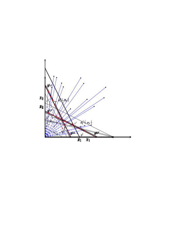
Figure 2. Choices that satisfy GAPP but not GARP

These choices, as shown in Figure 2, violate GARP as $p^{t}\cdot x^{t}=5>2=p^{t}\cdot x^{t^{\prime}}$ ($x^{t}\succ_{x}x^{t^{\prime}}$) and $p^{t^{\prime}}\cdot x^{t^{\prime}}=8>6=p^{t^{\prime}}\cdot x^{t}$ ($x^{t^{\prime}}\succ_{x}x^{t}$). However, these choices satisfy GAPP as $p^{t^{\prime}}\cdot x^{t^{\prime}}=8>2=p^{t}\cdot x^{t^{\prime}}$ ($p^{t}\succ_{p}p^{t^{\prime}}$) but $p^{t}\cdot x^{t}=5\ngeq 6=p^{t^{\prime}}\cdot x^{t}$ ($p^{t^{\prime}}\nsucceq_{p}p^{t}$).

While GAPP and GARP are not in general the same conditions, they coincide in any data set where $p^{t}\cdot x^{t}=1$ for all $t\in T$. This is because $x^{t}\succeq_{x}(\succ_{x})x^{t^{\prime}}$ if and only if $p^{t}\succeq_{p}(\succ_{p})p^{t^{\prime}}$ since both conditions are equivalent to $1\geq(>)\,p^{t}\cdot x^{t^{\prime}}$. Given a data set ${\mathcal{D}}=\{(p^{t},x^{t})\}_{t=1}^{T}$, we define the iso-expenditure version of $\mathcal{D}$ as another data set $\breve{\mathcal{D}}:=\left\{(p^{t},\breve{x}^{t})\right\}_{t=1}^{T}$, such that $\breve{x}^{t}=x^{t}/(p^{t}\cdot x^{t})$. This new data set has the feature that $p^{t}\cdot\breve{x}^{t}=1$ for all $t\in T$. Notice that the revealed price preference relations $\succeq_{p}$, $\succ_{p}$ remain unchanged when consumption bundles are scaled. Thus a data set obeys GAPP if and only if its iso-expenditure version obeys GAPP, which in this case is equivalent to GARP. The next proposition gives a more detailed statement of these observations.

Proposition 1

Let ${\mathcal{D}}=\{(p^{t},x^{t})\}_{t=1}^{T}$ be a data set and let $\breve{\mathcal{D}}=\{(p^{t},\breve{x}^{t})\}_{t\in T}$, where $\breve{x}^{t}=x^{t}/(p^{t}\cdot x^{t})$. Then the revealed preference relations $\succeq_{p}^{*}$ and $\succ_{p}^{*}$ on ${\mathcal{P}}=\{p^{t}\}_{t=1}^{T}$ and the revealed preference relations $\succeq_{x}^{*}$ and $\succ_{x}^{*}$ on ${\breve{\mathcal{X}}}=\{\breve{x}^{t}\}_{t=1}^{T}$ are related in the following manner:

1. $p^{t}\succeq^{*}_{p}p^{t^{\prime}}$ if and only if $\breve{x}^{t}\succeq^{*}_{x}\breve{x}^{t^{\prime}}$.

2. $p^{t}\succ^{*}_{p}p^{t^{\prime}}$ if and only if $\breve{x}^{t}\succ^{*}_{x}\breve{x}^{t^{\prime}}$.

As a consequence, $\mathcal{D}$ obeys GAPP if and only if its iso-expenditure version, $\breve{\mathcal{D}}$, obeys GARP.

Proof.  Notice that

$$p^{t}\cdot\frac{x^{t}}{p^{t}\cdot x^{t}}\geq p^{t}\cdot\frac{x^{t^{\prime}}}{p^{t^{\prime}}\cdot x^{t^{\prime}}}\,\iff\,p^{t^{\prime}}\cdot x^{t^{\prime}}\geq p^{t}\cdot x^{t^{\prime}}.$$

The left side of the equivalence says that $\breve{x}^{t}\succeq_{x}\breve{x}^{t^{\prime}}$ while the right side says that $p^{t}\succeq_{p}p^{t^{\prime}}$. This implies (1) since $\succeq_{p}^{*}$ and $\succeq_{x}^{*}$ are the transitive closures of $\succeq_{p}$ and $\succeq_{x}$ respectively. Similarly, it follows from

$$p^{t}\cdot\frac{x^{t}}{p^{t}\cdot x^{t}}>p^{t}\cdot\frac{x^{t^{\prime}}}{p^{t^{\prime}}\cdot x^{t^{\prime}}}\,\iff\,p^{t^{\prime}}\cdot x^{t^{\prime}}>p^{t}\cdot x^{t^{\prime}}$$

that $\breve{x}^{t}\succ_{x}\breve{x}^{t^{\prime}}$ if and only if $p^{t}\succ_{p}p^{t^{\prime}}$, which leads to (2). The claims (1) and (2) together guarantee that there is a sequence of observations in $\mathcal{D}$ that lead to a GAPP violation if and only if the analogous sequence in $\breve{\mathcal{D}}$ lead to a GARP violation. $\blacksquare$

As an illustration, compare the data sets in Figure 1 and Figure 2 to the iso-expenditure data sets in Figure 3a and Figure 3b. It can be clearly observed that the iso-expenditure data in Figure 3a contains a GARP violation (which implies it does not satisfy GAPP) whereas the data in Figure 3b does not violate GARP (and, hence, satisfies GAPP).

a Example 1

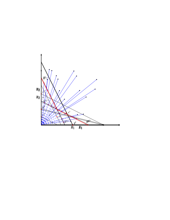
b Example 2

Figure 3. Expenditure-Normalized Choices

A consequence of Proposition 1 is that the augmented utility model can be tested in two ways: we can either test GAPP directly or we can test GARP on its iso-expenditure version. If we are simply interested in testing GAPP on a single-agent data set $\mathcal{D}$, normalization brings no advantage: the test is computationally straightforward in either case and involves the construction of their (respective) revealed preference relations and checking for acyclicity. However, as we shall see in Section 5, iso-expenditure scaling plays an important role in the test we develop (on repeated cross-sectional demand data) for the random utility version of the augmented utility model.

While GARP and GAPP are distinct properties, they are not mutually exclusive and it is possible for a data set to satisfy both. For example, if $\mathcal{D}=\{(p^{t},x^{t})\}_{t=1}^{T}$ is collected from a consumer who is maximizing a quasilinear augmented utility function, then it will satisfy both GAPP and GARP. When both properties are satisfied, then an analyst could make use of either property when making predictions of demand at an out-of-sample price; the two properties will then typically lead to different set predictions. We discuss this in greater detail in Section A.1 of the online appendix, which also contains more discussion of the relationship between revealed preferences under GAPP and under GARP.

In light of Proposition 1 and the fact that the revealed price preference relation is not affected by scaling consumption bundles, it is natural to wonder about the relationship between the testable implications of the augmented-utility model and the constrained-optimization model (as in (3)) restricted to homothetic preferences. A data set that can be rationalized in the latter sense will have the feature that it must satisfy GARP for any arbitrary scaling of consumption bundles and thus will satisfy GAPP. By contrast, a data set that satisfies GAPP must only satisfy GARP for the particular scaling that equalizes expenditure across observations. In other words, GAPP is a less stringent property; that it is strictly less stringent is clear from Example 2, which satisfies GAPP but violates GARP and therefore cannot be rationalized in Afriat’s sense (as given by (3)) for any locally nonsatiated preference, let alone a homothetic preference.

3.2. Preference over Prices

We know from Theorem 1 that if $\mathcal{D}$ obeys GAPP then it can be rationalized by an augmented utility function with an indirect utility that is defined at all price vectors in $\mathbb{R}_{++}^{L}$. It is straightforward to check that any indirect utility function $V$ as defined by (1) has the following two properties:

• it is nonincreasing in $p$, in the sense that if $p^{\prime}\geq p$ (element by element) then $V(p^{\prime})\leq V(p)$, and

• it is quasiconvex in $p$, in the sense that if $V(p)=V(p^{\prime})$, then $V(\beta p+(1-\beta)p^{\prime})\leq V(p)$ for any $\beta\in[0,1]$.

Any rationalizable data set $\mathcal{D}$ could potentially be rationalized by many augmented utility functions, with each one leading to a different indirect utility function. We denote this set of indirect utility functions by $\mathbf{V}({\mathcal{D}})$. We have already observed that if $p^{t}\succeq_{p}^{*}(\succ_{p}^{*})\,p^{t^{\prime}}$ then $V(p^{t})\geq(>)\,V(p^{t^{\prime}})$ for any $V\in\mathbf{V}({\mathcal{D}})$; in other words, the conclusion that the consumer prefers the prices $p^{t}$ to $p^{t^{\prime}}$ is nonparametric in the sense that it is independent of the precise augmented utility function used to rationalize $\mathcal{D}$. The next result (proved in Appendix A.2) says that, without further information on the augmented utility function, this is all the information on the consumer’s preference over prices in $\mathcal{P}$ that we can glean from the data. Thus, in our nonparametric setting, the revealed price preference relation contains the most detailed information for welfare comparisons.

Proposition 2

Suppose ${\mathcal{D}}=\{(p^{t},x^{t})\}_{t=1}^{T}$ is rationalizable by an augmented utility function. Then for any $p^{t}$, $p^{t^{\prime}}$ in $\mathcal{P}$:

1. $p^{t}\succeq^{*}_{p}p^{t^{\prime}}$ if and only if $V(p^{t})\geq V(p^{t^{\prime}})$ for all $V\in\mathbf{V}({\mathcal{D}})$.

2. $p^{t}\succ_{p}^{*}p^{t^{\prime}}$ if and only if $V(p^{t})>V(p^{t^{\prime}})$ for all $V\in\mathbf{V}({\mathcal{D}})$.

3.3. Compensation for a price change

In standard consumer theory, the compensating and equivalent variations are two ways of quantifying the welfare impact of a price change (see Mas-Colell, Whinston, and Green (1995), Chapter 3.I). We now argue that analogues exist for the augmented utility model and that bounds for them can be recovered from the data.

Let $U$ be the consumer’s augmented utility function. Suppose that the initial price is $p^{t_{1}}$ and it changes to $p^{t_{2}}$, leading to a change in consumption from $x^{t_{1}}$ to $x^{t_{2}}$. Then we can find $\mu_{c}$ such that

$$\max\nolimits_{x\in\mathbb{R}_{+}^{L}}U(x,-p^{t_{2}}\cdot x-\mu_{c})=V(p^{t_{1}}).$$ (8)

Note that $\mu_{c}$ is unique since $U$ is strictly increasing in the last argument. We could think of $\mu_{c}$ as the lump sum transferred from the consumer (if it is positive) or to the consumer (if it is negative) after the price change that will make her just indifferent between the situation before and after the change.

Suppose we interpret $U$ as arising from an overall utility function $\widetilde{U}(x,z)$ (that depends on the observed goods $x$ and the level $z$ of an outside good), given the consumer’s wealth of $M$, so that $U(x,-e)=\widetilde{U}(x,M-e)$. Since $\mu_{c}$ solves (8), it will also satisfy

$$\max\nolimits_{\{x\in\mathbb{R}_{+}^{L}:\;p^{t_{2}}\cdot x\leq M-\mu_{c}\}}\widetilde{U}(x,(M-\mu_{c})-p^{t_{2}}\cdot x)\;=\;\widetilde{U}(x^{t_{1}},M-p^{t_{1}}\cdot x^{t_{1}}).$$

In other words, $\mu_{c}$ is the reduction in total wealth that will leave the consumer’s overall utility at $p^{t_{2}}$ the same as it was at $p^{t_{1}}$. Thus, with this particular interpretation of the augmented utility function, $\mu_{c}$ coincides with what is called the compensating variation in standard consumer theory. For this reason, we shall also refer to $\mu_{c}$, defined by (8), as the compensating variation.

Pushing the analogy further, it is possible to use the compensating variation in our model in the same way it is typically used. For example, the price change from $p^{t_{1}}$ to $p^{t_{2}}$ may benefit some consumers while hurting others. The Kaldor criterion would deem this change an overall improvement if the sum of the compensating variations across all consumers is positive since it guarantees that those who benefit from the price change could, in principle, compensate the losers and still be better off.

In a similar way, we can define the equivalent variation as the value $\mu_{e}$ that solves

$$\max\nolimits_{x\in\mathbb{R}_{+}^{L}}U(x,-p^{t_{1}}\cdot x+\mu_{e})=V(p^{t_{2}})$$ (9)

If $U(x,-e)=\widetilde{U}(x,M-e)$ then $\mu_{e}$ also solves

$$\max\nolimits_{\{x\in\mathbb{R}_{+}^{L}:\;p^{t_{2}}\cdot x\leq M+\mu_{e}\}}\widetilde{U}(x,(M+\mu_{e})-p^{t_{1}}\cdot x)=\widetilde{U}(x^{t_{2}},M-p^{t_{2}}\cdot x^{t_{2}}).$$

In other words, $\mu_{e}$ coincides with the equivalent variation as it is usually defined.

Now suppose a data set $\mathcal{D}$ obeys GAPP and contains the observation $(p^{t_{1}},x^{t_{1}})$. What can we say about the compensating variation of a price change from $p^{t_{1}}$ to $p^{t_{2}}$ (where the latter may or may not be a price observed in $\mathcal{D}$)? There will typically be a range of these values since there is more than one augmented utility function that rationalizes $\mathcal{D}$. Nonetheless, it is possible to obtain a tight lower bound for the set of possible compensating variation values. Formally, this is given by

$$\inf\{\mu_{c}:\mbox{$\mu_{c}$ solves (\ref{CV}) for some augmented utility function $U$ that rationalizes $\mathcal{D}$}\}.$$

Abusing terminology somewhat, we shall denote this term simply by $\inf({\mu}_{c})$.

We now describe how to compute this bound. Let $S\subset T$ be the set of observations such that $s\in S$ if $p^{s}\succeq^{*}_{p}p^{t_{1}}$. This set is nonempty since it contains $p^{t_{1}}$ itself. For each $s\in S$, there is $m_{c}^{s}$ such that

$$p^{t_{2}}\cdot x^{s}+m_{c}^{s}=p^{s}x^{s}.$$ (10)

We claim that for any $U$ that rationalizes $\mathcal{D}$, the compensating variation $\mu_{c}\geq m_{c}^{s}$. This is because if $m<m_{c}^{s}$, then $m\neq\mu_{c}$ for any utility function rationalizing $\mathcal{D}$. Indeed,

$$\max\nolimits_{x\in\mathbb{R}_{+}^{L}}U(x,-p^{t_{2}}\cdot x-m)\geq U(x^{s},-p^{t_{2}}\cdot x^{s}-m)>U(x^{s},-p^{t_{2}}\cdot x^{s}-m_{c}^{s})\\ =U(x^{s},-p^{s}\cdot x^{s})\geq U(x^{t_{1}},-p^{t_{1}}\cdot x^{t_{1}})=V(p^{t_{1}}).$$

Thus $\inf(\mu_{c})\geq m_{c}^{s}$ for all $s\in S$. In fact, it is possible to obtain a stronger conclusion:

$$\inf(\mu_{c})=\max\{m_{c}^{s}:\mbox{$m_{c}^{s}$ satisfies (\ref{justnice}) for some $s\in S$}\}.$$ (11)

Since the right side of this equation can be easily computed from the data, we have found a practical way of calculating $\inf(\mu_{c})$.

Notice that if $p^{t_{2}}$ is revealed preferred to $p^{t_{1}}$ (equivalently, that there is $s^{\prime}\in S$ such that $m_{c}^{s^{\prime}}\geq 0$), then $\inf(\mu_{c})\geq 0$; in other words, at $p=p^{t_{2}}$, a lump sum tax of $\inf(\mu_{c})$ will leave the agent no worse off than at $t_{1}$ and potentially better off. On the other hand, if $p^{t_{2}}$ is not revealed preferred to $p^{t_{1}}$, that is, for every $s\in S$, we have $m_{c}^{s}<0$, then $\inf(\mu_{c})<0$; in other words, at $p=p^{t_{2}}$, a lump sum transfer of $\inf(\mu_{c})$ to the agent will leave the agent no worse off than at $t_{1}$ and potentially better off.

We provide a fuller discussion on the compensating variation, including a proof of (11), in Appendix A.5.

3.4. Measuring departures from rationality

Empirical studies that apply Afriat’s Theorem frequently find GARP violations. A common way of measuring the extent of such violations is to compute the critical cost efficiency index Afriat (1973). This refers to the largest $e\in(0,1]$ such that $\mathcal{D}$ can be rationalized in the following sense: there is a locally-nonsatiated utility function $\widetilde{U}$ such that $\widetilde{U}(x^{t})\geq\widetilde{U}(x)$ for all $x$ in the ‘shrunken’ budget set $B^{t}_{e}=\left\{x\in\mathbb{R}_{+}^{L}:\;p^{t}\cdot x\leq ep^{t}\cdot x^{t}\right\}$. Rationality is imperfect if $e<1$ since the consumer behaves as though she ignores bundles $x^{\prime}$ that satisfy $ep^{t}\cdot x^{t}<p^{t}\cdot x^{\prime}\leq p^{t}\cdot x^{t}$ and, there could be some observation $\hat{t}$ and bundle $x^{\prime}$ in this range for which $\widetilde{U}(x^{\prime})>\widetilde{U}(x^{\hat{t}})$. Importantly, the calculation of the critical cost efficiency index is straightforward and is facilitated by a modified version of GARP.

There is a similar way of measuring the extent to which a data set $\mathcal{D}$ fails to be rationalized by an augmented utility function. For a given $\vartheta\in(0,1]$, there is a weaker version of the GAPP test that allows us to determine whether there is an expenditure-augmented utility $U:\mathbb{R}_{+}^{L}\times\mathbb{R}_{-}\to\mathbb{R}$ such that, at each observation $t$,

$$U(x^{t},-p^{t}\cdot x^{t})\geq U(x,-\vartheta^{-1}p^{t}\cdot x)\>\mbox{ for all $x\in\mathbb{R}_{+}^{L}$.}$$

If there is, we say that $\mathcal{D}$ is $\vartheta$-rationalized by an augmented utility function. Notice that if $\mathcal{D}$ can be $\vartheta$-rationalized then it can be $\vartheta^{\prime}$-rationalized for any $\vartheta^{\prime}<\vartheta$, since $U$ is strictly decreasing in expenditure. The consumer who is $\vartheta$-rational (for $\vartheta<1$) may have only limited or bounded rationality in the sense that there could be a bundle $x^{\prime}$ and an observation $\hat{t}$ such that

$$U(x^{\hat{t}},-p^{\hat{t}}\cdot x^{\prime})>U(x^{\hat{t}},-p^{\hat{t}}\cdot x^{\hat{t}})\geq U(x^{\prime},-\vartheta^{-1}p^{\hat{t}}\cdot x^{\prime}).$$

In other words, the consumer fails to recognize that bundle $x^{\prime}$ is superior to $x^{\hat{t}}$ at $t=\hat{t}$ because she has inflated (by $\vartheta^{-1}$) the expenditure of purchasing $x^{\prime}$. Any data set can be $\vartheta$-rationalized for some $\vartheta\in(0,1]$ and the supremum $\vartheta^{*}$ over these values provides a natural measure of rationality which we shall refer to as the rationality index.

The following proposition establishes a connection of our rationality index with the critical cost efficiency index.

Proposition 3

Let ${\mathcal{D}}=\{(p^{t},x^{t})\}_{t=1}^{T}$ be a data set and let $\breve{\mathcal{D}}=\{(p^{t},\breve{x}^{t})\}_{t\in T}$, where $\breve{x}^{t}=x^{t}/(p^{t}\cdot x^{t})$, be its iso-expenditure version. Then $\vartheta^{*}$ is the rationality index for $\mathcal{D}$ if and only if it is the critical cost efficiency index for $\breve{\mathcal{D}}$.

A consequence of this result is that the rationality index inherits the ease of computation of the critical cost efficiency index. In Appendix A.4.2, we provide instructions on this computation including in more general environments with nonlinear prices. The proof of Proposition 3 can be found in Appendix A.4.3.

3.5. Deflating prices

When the data set $\mathcal{D}=\{(p^{t},x^{t})\}_{t=1}^{T}$ is collected over an extended period, it is possible that there are changes in the prices of all goods, including goods outside the ones observed. Thus the nominal value of expenditure may no longer be an accurate measure of the opportunity cost of expenditure. A simple way of taking this into account is to deflate the prices of the $L$ goods with a general price index. In other words, one could check if $\widetilde{\mathcal{D}}=\{(p^{t}/k^{t},x^{t})\}_{t=1}^{T}$ obeys GAPP, where $k^{t}\in\mathbb{R}_{++}$ is an index of the general price level. If it does, it would mean that there is an augmented utility function $U$ that rationalizes the data after deflation; in other words,

$$x^{t}\in\operatornamewithlimits{argmax}_{x\in\mathbb{R}^{L}_{+}}U\left(x,-\frac{p^{t}\cdot x}{k^{t}}\right)\>\mbox{ for all $t\in T$.}$$

This simple way of accounting for general price changes could be precisely justified when the augmented utility function is the reduced form of a larger constrained optimization problem. Indeed, suppose that the consumer is maximizing an overall utility $\widetilde{U}(x,y)$ that depends both on the observed bundle $x$ and on a bundle $y$ of other goods, subject to a global budget of $M$. Formally, the consumer maximizes $\widetilde{U}(x,y)$ subject to $p\cdot x+q\cdot y\leq M$, where $q$ are the prices of goods $y$. Keeping $q$ and $M$ fixed, $U(x,-e)$ is defined as the greatest overall utility the consumer can achieve by choosing $y$ optimally, subject to expenditure $M-e$ and conditional on consuming $x$, that is,

$$U(x,-e)=\max\{\widetilde{U}(x,y):\mbox{$y\geq 0$ and $q\cdot y\leq M-e$}\}.$$ (12)

At the prices $p^{t}$ for the observed goods and $q$ for the outside goods, the consumer chooses a bundle $(x^{t},y^{t})$ to maximize $\widetilde{U}$ subject to $p^{t}\cdot x+q\cdot y\leq M$. Then $\mathcal{D}=\{(p^{t},x^{t})\}_{t=1}^{T}$ will obey GAPP, since $x^{t}$ maximizes $U(x,-p^{t}\cdot x)$, with $U$ as defined by (12).

Now suppose that the prices of the other goods are changing. Consider the simplest case where these prices move up or down proportionately, so they are $k^{t}q$ at observation $t$, for some scalar $k^{t}>0$. Furthermore, assume that the agent’s global budget at $t$ also increases by a factor $k^{t}$, which means that the consumer’s nominal wealth is keeping pace with price inflation. Then at observation $t$, the consumer maximizes $\widetilde{U}(x,y)$ subject to $(x,y)$ obeying

$$p^{t}\cdot x+k^{t}q\cdot y\leq k^{t}M.$$

Dividing this inequality by $k^{t}$, we see that the consumer’s choice is identical to the case where the price of the observed goods is $p^{t}/k^{t}$, with external prices and total wealth constant at $q$ and $M$ respectively. Therefore, the data set with deflated prices, $\widetilde{\mathcal{D}}=\{(p^{t}/k^{t},x^{t})\}_{t=1}^{T}$ obeys GAPP.

In the case where the relative prices of the outside goods change, it is still possible to derive a price index which ensures that GAPP holds after deflating $p^{t}$, but this requires stronger assumptions on $\widetilde{U}$. We discuss this in detail in Appendix A.3.

4. General consumption spaces and nonlinear pricing

So far we have assumed that the consumption space is $\mathbb{R}^{L}_{+}$ and that prices are linear, but in fact neither feature is crucial to our main result. In this section, we assume that the space from which the consumer chooses her consumption is $X\subseteq\mathbb{R}_{+}^{L}$. We define a price system as a map $\psi:X\to\mathbb{R}_{+}$, where $\psi(x)$ is the cost of purchasing $x\in X$. Of course, a special case of a price system is $\psi(x)=p\cdot x$ but the more general formulation with $\psi$ allows for quantity discounts, bundle pricing and other pricing features that can be important in certain contexts (such as our empirical application in Section 7.1).

We assume that both the price system and the bundle chosen by the consumer are observed. Formally, a data set is a collection $\mathcal{D}=\{(\psi^{t},x^{t})\}_{t=1}^{T}$. This data set is rationalized by an augmented utility function $U:X\times\mathbb{R}_{-}\to\mathbb{R}$ if

$$x^{t}\in\operatornamewithlimits{argmax}_{x\in X}U(x,-\psi^{t}(x))\>\mbox{ for all $t\in T$.}$$ (13)

The notion of revealed preference over prices can be extended to a revealed preference over price systems. We say that $\psi^{t^{\prime}}$ is directly revealed preferred (directly revealed strictly preferred) to $\psi^{t}$ if $\psi^{t^{\prime}}(x^{t})\leq(<)\psi^{t}(x^{t})$; we denote this by $\psi^{t^{\prime}}\succeq_{p}(\succ_{p})\psi^{t}$. We denote the transitive closure of $\succeq_{p}$ by $\succeq_{p}^{*}$, that is, $\psi^{t^{\prime}}\succeq_{p}^{*}\psi^{t}$ if there are $t_{1}$, $t_{2},\ldots,t_{N}$ in $T$ such that $\psi^{t^{\prime}}\succeq_{p}\psi^{t_{1}}$, $\psi^{t_{1}}\succeq_{p}\psi^{t_{2}},\ldots,\psi^{t_{N-1}}\succeq_{p}\psi^{t_{N}}$, and $\psi^{t_{N}}\succeq_{p}\psi^{t}$; in this case we say that $\psi^{t^{\prime}}$ is revealed preferred to $\psi^{t}$. If anywhere along this sequence, it is possible to replace $\succeq_{p}$ with $\succ_{p}$ then we denote that relation by $\psi^{t^{\prime}}\succ^{*}_{p}\psi^{t}$ and say that $\psi^{t^{\prime}}$ is strictly revealed preferred to $\psi^{t}$. It is straightforward to check that if, $\mathcal{D}$ can be rationalized by an augmented utility function, then it obeys the following generalization of GAPP to price systems:

there do not exist observations $t,t^{\prime}\in T$ such that $\psi^{t^{\prime}}\succeq^{*}_{p}\psi^{t}$ and $\psi^{t}\succ^{*}_{p}\psi^{t^{\prime}}$.

The following theorem asserts that the converse is also true and that, under further conditions, we can guarantee that the data can be rationalized by an augmented utility function with additional properties. The proof of this result (in fact of a more general result allowing for errors) is in Appendix A.4.1.

Theorem 2

A data set $\mathcal{D}=\{(\psi^{t},x^{t})\}^{T}_{t=1}$ can be rationalized by an augmented utility function if and only if satisfies GAPP.

Furthermore, suppose that $\mathcal{D}$ satisfies GAPP, $X$ is closed and that, for all $t\in T$, the price systems have the following properties:  (i) $\psi^{t}$ is a continuous function; (ii) for any number $M$, $\{x\in X:\psi^{t}(x)\leq M\}$ is a compact set; and (iii) $\psi^{t}$ is strictly increasing in $x_{K}$ for some $K\subseteq L$. Then, for any closed set $Y\subseteq\mathbb{R}^{L}_{+}$ containing $X$, there is a continuous augmented utility function $U:Y\times\mathbb{R}_{-}\to\mathbb{R}$ that rationalizes $\mathcal{D}$, with $U(x,-e)$ strictly increasing in $x_{K}$.

Remarks:  (1)  Note that condition (ii) is a weak assumption requiring that there be no arbitrarily large bundles with a bounded price. (2) By definition, an augmented utility function is strictly decreasing in expenditure, but in certain cases it may be natural to require $U$ to be strictly increasing in $x_{K}$ for some set $K$ (which can be empty). The theorem says that this is possible, so long as the price systems are also strictly increasing in $x_{K}$. (3) Lastly, the theorem guarantees that the domain of the augmented utility function can be larger than $X$. For reasons which will be clear later in this section, this is natural in certain applications. However when we say that $U$ rationalizes the data, we mean that (13) holds and, in particular, $x^{t}$ need not be optimal in $Y$.

The literature on mental accounting has emphasized the possibility of actors in the economy manipulating the mental budgets of agents. The following example shows how a nonlinear GAPP test can be used to detect such phenomena.

Example 3.

A store initially prices two goods at $p^{t}=(1,2)$ and a shopper purchases $x^{t}=(10,20)$ from the store. The store introduces a scheme where regular customers (such as this shopper) receives a voucher of 12 dollars to be used for the purchase of the store’s products; prices are changed to $p^{t^{\prime}}=(2,3/2)$ and the shopper buys $x^{t^{\prime}}=(20,20)$. What is the impact of the gift voucher?

Since the value of the voucher is small in terms of total income, the shopper could spread this reward widely across all purchases (including purchases from other stores) and this should result in no (or at least a very small) impact on demand for the store’s products. On the other hand, she may have a mental budget for purchases at that store, and the voucher represents an appreciable increase in that mental budget by 12 dollars.

A revealed preference analysis supports the latter hypothesis. Indeed, if we ignore the voucher, the data are not compatible with the maximization of an augmented utility function since $p^{t}\cdot x^{t}=50=p^{t^{\prime}}\cdot x^{t}$ and $p^{t^{\prime}}\cdot x^{t^{\prime}}=70>60=p^{t}\cdot x^{t^{\prime}}$, which violates GAPP. On the other hand, at observation $t^{\prime}$, we could model the shopper as mentally discounting 12 dollars from her expenditure at the shop. In formal terms, the price system at $t^{\prime}$ is a function $\psi^{t^{\prime}}(x)=\max\{p^{t^{\prime}}\cdot x-12,0\}$, so $\psi^{t^{\prime}}(x^{t^{\prime}})=58$. In this case, we have $\psi^{t^{\prime}}\succ^{*}_{p}\psi^{t}$ (where $\psi^{t}(x)=p^{t}x$), but it is no longer the case that $\psi^{t}\succeq^{*}_{p}\psi^{t^{\prime}}$ since $\psi^{t}(x^{t^{\prime}})=60>\psi^{t^{\prime}}(x^{t^{\prime}})=58$. So the data is now compatible with GAPP, but with a nonlinear pricing system based on the shopper’s mental accounting.

4.1. Discrete consumption spaces

Below are four instances where Theorem 2 could be applied.

(1)  Suppose that the consumption space consists of $L$ goods of which the first $K$ can only be consumed in discrete quantities (as in the model of Polisson and Quah (2013), for example). The consumption space is then $X=\mathbb{N}^{K}\times\mathbb{R}^{L-K}_{+}$, where $\mathbb{N}$ is the set of natural numbers. Theorem 2 is applicable whether or not prices are linear. Suppose that each good has a price $p_{i}>0$. Since $X$ is closed and the price system $\psi^{t}(x)=p^{t}\cdot x$ is strictly increasing in $x$, Theorem 2 guarantees that, if GAPP holds, then there is a continuous augmented utility function that is strictly increasing in $x\in X$ and rationalizes $\mathcal{D}$.

(2)  Another natural choice environment is one where the consumer is deciding on buying a subset of objects from a set with $L$ items. Then each subset could be represented as an element of $X=\{0,1\}^{L}$. For $x\in X$, the $\ell^{\text{th}}$ entry $x_{\ell}$ equals 1 if and only if the $\ell^{\text{th}}$ object is chosen. If only certain subsets are permissible, as in the case of discrete choice, then $X$ would be a strict subset of $\{0,1\}^{L}$. The price system $\psi$ gives the price of different bundles of goods. Let $e_{\ell}$ denote the vector with 1 in the $\ell^{\text{th}}$ entry and zero everywhere else. Then $\psi(e_{\ell})$ is the price of purchasing good ${\ell}$ alone. The price system is nonlinear if $\psi(x)\neq\sum_{\ell=1}^{L}x_{\ell}\psi(e_{\ell})$ for some $x\in X$.

(3)  In empirical models of demand for differentiated goods, it is common to model each good as embodying a set of characteristics (see Nevo (2000)). For example, if each good is a type of breakfast cereal, then the characteristics could be the calories, fiber content etc. Suppose that there are $L$ characteristics and let $Y_{\ell}\subseteq\mathbb{R}_{+}$ be the set of values that characteristic $\ell$ can take. Then, the characteristics space is $Y=\times_{\ell=1}^{L}Y_{\ell}$. There are $I$ goods, with good $i$ having characteristics $x^{i}\in Y$. Assuming (as is common in these models) that a consumer purchases only one good, the consumption space is $X=\{x^{i}\}_{i=1}^{I}$ and a price system $\psi:X\to\mathbb{R}_{++}$ is just a list of prices for the different goods.

In this context, it is natural to model the consumer with an augmented utility function defined on characteristics and expenditures $Y\times\mathbb{R}_{-}$, even though the products available to her are only those in $X$. Furthermore, among the characteristics, there could be those where higher values are unambiguously better, in which case the researcher could be interested in guaranteeing that utility is strictly increasing in those characteristics. Theorem 2 allows for these considerations. If $\mathcal{D}$ obeys GAPP then it can be rationalized by a continuous augmented utility function $U:Y\times\mathbb{R}_{-}\to\mathbb{R}$. Additionally, for a set of characteristics $K\subseteq L$, one could guarantee that $U(y,-e)$ is strictly increasing in $y_{K}$ so long as $\psi^{t}(x)$ is strictly increasing in $x_{K}$, for all $t$.

In models of differentiated goods, it is also common to allow for the introduction of new goods and for changes to a product’s characteristics. Obviously, changes to a product’s characteristics could potentially lead to a change in the product’s utility which, unless taken into account by the test, could lead to a spurious rejection of augmented utility-maximization. In formal terms, these changes can be captured by allowing the set of alternatives to depend on $t$; in Section A.4.4, we explain how it is possible to modify the GAPP test in Theorem 2 to account for changes of this type.

4.2. Characteristics models with continuous consumption spaces

We assume that the space of characteristics is $Y=\mathbb{R}^{L}_{+}$, with each product $i$ represented by a vector of characteristics $x^{i}\in Y$. We allow these goods to be bought in bundles, so the consumption space is the convex cone $X$ generated by $\{x^{i}\}_{i=1}^{I}$. We assume that the vectors $\{x^{i}\}_{i=1}^{I}$ are linearly independent; this guarantees that for each $\hat{x}\in X$, there is a unique bundle of goods, $\hat{\alpha}=(\hat{\alpha}_{i})_{i=1}^{I}\in\mathbb{R}^{I}_{+}$ such that $\sum_{i=1}^{I}\hat{\alpha}_{i}x^{i}=\hat{x}$. We denote $\hat{\alpha}$ by $\alpha(\hat{x})$. Let $p^{t}\in\mathbb{R}^{I}_{++}$ be the prices of the $I$ goods at observation $t$. To obtain the bundle $x\in X$, the consumer needs to spend $\psi^{t}(x)=p^{t}\cdot\alpha(x)$.

At observation $t$, the researcher observes $p^{t}$ and the consumer’s purchases $\alpha^{t}\in\mathbb{R}^{I}_{+}$. We assume the researcher knows $\{x^{i}\}_{i=1}^{I}$ and so he can work out the consumption in characteristics space, $x^{t}=\sum_{i=1}^{I}\alpha^{t}_{i}x^{i}$, as well as the price system $\psi^{t}$. Theorem 2 guarantees that if $\mathcal{D}=\{(\psi^{t},x^{t})\}_{t\in T}$ satisfies GAPP then it can be rationalized by a continuous augmented utility function $U:\mathbb{R}^{L}_{+}\times\mathbb{R}_{-}\to\mathbb{R}$. So long as $\psi^{t}(x)$ is strictly increasing in $x\in X$ for each $t$, we can also ensure that $U(y,-e)$ is increasing in the characteristics $y$.

5. The Random Augmented Utility Model

In this section, we develop the random version of the expenditure-augmented utility model. We first describe our test procedure for this model via a simple example.

5.1. An Illustrative Example

Example 4.

Suppose we have repeated cross-sectional data consisting of the demand of a population of ten consumers at two price vectors. This is illustrated in Figure 4 where the collection of points in the left and right panels indicate the demand bundles at $p^{t}=(2,1)$ and $p^{t^{\prime}}=(1,2)$ respectively. The lines in Figure 4 indicate relative prices.

a Choices under prices $p^{t}$

b Choices under prices $p^{t^{\prime}}$

Figure 4. The Data Set

Since we assume this is a cross-sectional data set, the econometrician cannot match consumption bundles across the two panels by consumer identity. The question we wish to address is whether this data set can be rationalized, by which we mean the following.

Can we match the choices at $t$ with those at $t^{\prime}$, forming ten distinct pairs, such that each pair can be rationalized by an augmented utility function (or, equivalently, satisfies GAPP)?

This exercise illustrates the problem we address in this section: given the empirical demand distributions in different periods, is there a time-invariant distribution over consumer types that could explain these empirical distributions, subject to the restriction that each type is an augmented utility function maximizer.

An obvious way of answering the above question would be to consider all possible partitions into pairs and test GAPP on each pair. This approach, however, is not practical when the population at each observation is large and when there are more than two periods. Fortunately, there is a different procedure that works in general, which we now explain.

Proposition 3 tells us that a pair $\mathcal{D}=\{(p^{t},x),(p^{t^{\prime}},x^{\prime})\}$ created by choosing bundle $x$ from observation $t$ and $x^{\prime}$ from observation $t^{\prime}$ obeys GAPP if and only if its iso-expenditure analog, $\breve{\mathcal{D}}=\{(p^{t},\breve{x}),(p^{t^{\prime}},\breve{x}^{\prime})\}$ obeys GARP, where $\breve{x}=x/p\cdot x$ and $\breve{x}^{\prime}=x^{\prime}/p\cdot x^{\prime}$ are scaled versions of $x$ and $x^{\prime}$ that satisfy $p^{t}\cdot\breve{x}=p^{t^{\prime}}\cdot\breve{x}=1$. This scaling is demonstrated in Figures 5a and 5b. Figure 5c shows the scaled bundles from both observations superimposed onto a single picture. This figure also labels different partitions of the budget lines and we use this notation in what follows.

a Period $t$

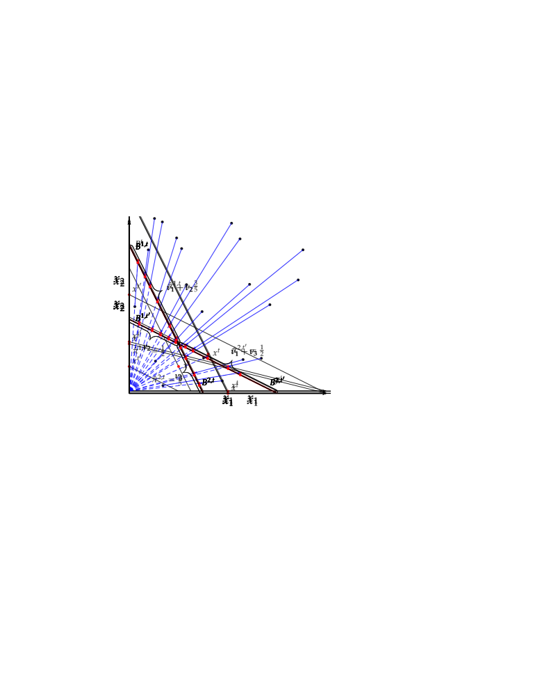
b Period $t^{\prime}$

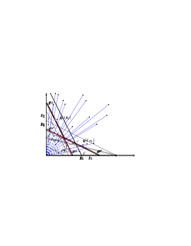
c Patches generated by budget intersections

Figure 5. Observed and Rescaled Choices

Now recall that, if $\breve{\mathcal{D}}$ satisfies GARP, then it is not possible for $\breve{x}$ to lie on $B^{2,t}$ and for $\breve{x}^{\prime}$ to lie on $B^{1,t^{\prime}}$ (see Figure 5(c)). Instead $\breve{\mathcal{D}}$ must belong to one of the following three types: $\breve{x}$ lies on $B^{1,t}$ and $\breve{x}^{\prime}$ lies on $B^{2,t^{\prime}}$; $\breve{x}$ lies on $B^{1,t}$ and $\breve{x}^{\prime}$ lies on $B^{1,t^{\prime}}$; or $\breve{x}$ lies on $B^{2,t}$ and $\breve{x}^{\prime}$ lies on $B^{2,t^{\prime}}$. These cases are graphically depicted in Figure 6a, Figure 6b and Figure 6c respectively.

a Proportion of this Rational Type: $\nu_{1}$

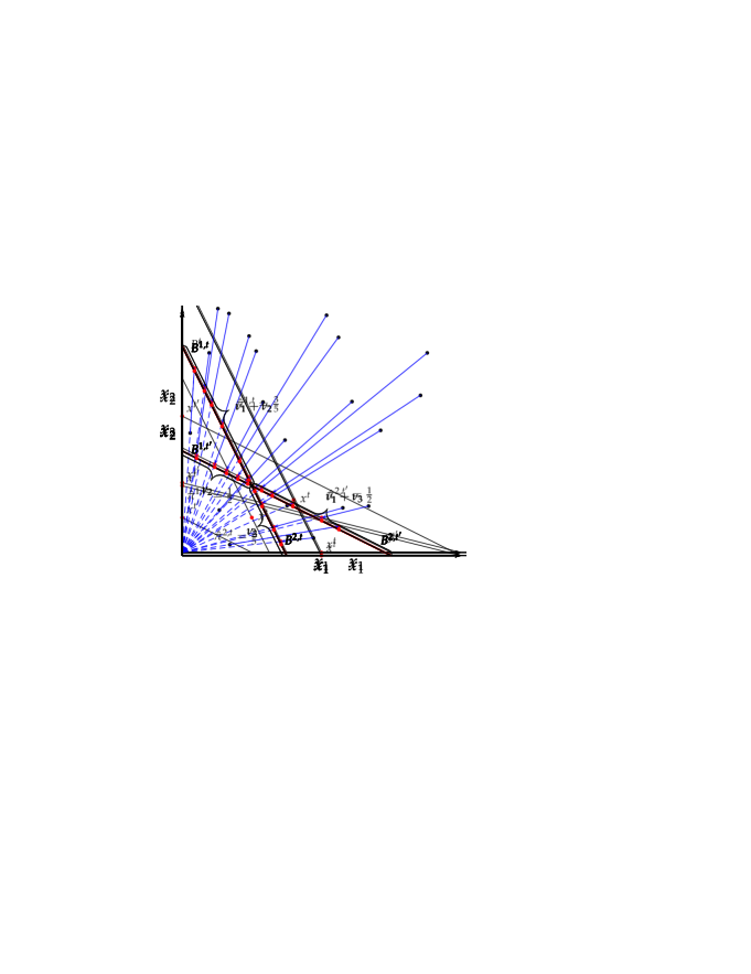
b Proportion of this Rational Type: $\nu_{2}$

c Proportion of this Rational Type: $\nu_{3}$

Figure 6. Set of Rational Types

Denoting the fraction of each of these GAPP-consistent consumer types in the population by $\nu_{1}$, $\nu_{2}$ and $\nu_{3}$ respectively, together they must generate the observed proportion of choices on the segments $B^{1,t},\;B^{2,t},\;B^{1,t^{\prime}}$ and $B^{2,t^{\prime}}$. Figure 7a demonstrates the proportion of choices in terms of the $\nu$s, while Figure 7b displays the empirical proportion of choices on each segment (after scaling), which we denote by

$$\hat{\pi}=\left(\hat{\pi}^{1,t},\hat{\pi}^{1,t^{\prime}},\hat{\pi}^{2,t},\hat{\pi}^{2,t^{\prime}}\right)^{\prime}=\left(\frac{3}{5},\frac{2}{5},\frac{1}{2},\frac{1}{2}\right)^{\prime}.$$ (14)

(For instance, $\hat{\pi}^{1,t}=\frac{3}{5}$ because six of the ten rescaled demand bundles lie on $B^{1,t}$.) Therefore, a necessary condition for rationalizing the data is that there are $\nu$s that solve

$$\nu_{1}+\nu_{2}=\hat{\pi}^{1,t},\;\nu_{1}+\nu_{3}=\hat{\pi}^{2,t^{\prime}},\;\nu_{2}=\hat{\pi}^{1,t^{\prime}},\;\nu_{3}=\hat{\pi}^{2,t}.$$ (15)

Two observations should be immediate from this process. The first is that there could be data where the system (15) has no solution; this occurs when $\hat{\pi}^{1,t}-\hat{\pi}^{1,t^{\prime}}\neq\hat{\pi}^{2,t^{\prime}}-\hat{\pi}^{2,t}$. The second is that when the values of $\hat{\pi}$ are given by (14), the solution to (15) is

$$\nu=(\nu_{1},\nu_{2},\nu_{3})^{\prime}=\left(\frac{1}{10},\frac{1}{2},\frac{2}{5}\right)^{\prime}.$$ (16)

To confirm that the data in this example can indeed be rationalized, it remains for us to pair up the demand bundles at the two observations. To do this, arbitrarily choose $1(=\nu_{1}\times 10)$ pair of choices that lie on $B^{1,t}$ and $B^{2,t^{\prime}}$; any 5 ($=\nu_{2}\times 10$) pairs that lie on $B^{1,t}$ and $B^{1,t^{\prime}}$; and the remaining 4 ($=\nu_{3}\times 10$) pairs on $B^{2,t}$ and $B^{2,t^{\prime}}$. Clearly each pair satisfies GARP and thus the original (un-scaled) pair satisfies GAPP.

a Resulting Distribution of Choices

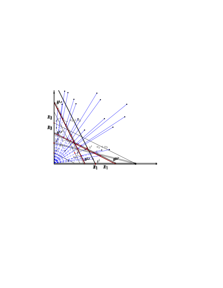
b The Scaled Empirical Choice Probabilities $\hat{\pi}$

Figure 7. Choice Distribution and Empirical Frequency

5.2. Rationalization by Random Augmented Utility

The starting point of our analysis is a repeated cross-sectional data set, $\mathscr{D}:=\{(p^{t},\mathring{\pi}^{t})\}_{t=1}^{T}$, where each observation consists of the prevailing price $p^{t}$ and the distribution of demand in the population at that price, represented by a probability measure $\mathring{\pi}^{t}$ on $\mathbb{R}^{L}_{+}$. An example of $\mathscr{D}$ is the data set depicted in Figure 4 where the probability measure corresponds to the empirical distribution of demand bundles. The following definition generalizes the notion of rationalization considered in that example.

Definition 5.1.

The repeated cross-sectional data set $\mathscr{D}=\{(p^{t},\mathring{\pi}^{t})\}_{t=1}^{T}$ is rationalized by the random augmented utility model (RAUM) if there exists a probability space $(\Omega,\mathcal{F},\mu)$ and a random variable $\chi:\Omega\to(\mathbb{R}^{L}_{+})^{T}$ such that, almost surely, $\{(p^{t},\chi^{t}(\omega))\}_{t\in T}$ can be rationalized by an augmented utility function (equivalently, obeys GAPP) and

$$\mathring{\pi}^{t}(Y)=\mu(\{\omega\in\Omega:\chi^{t}(\omega)\in Y\})\>\mbox{ for any measurable $Y\subseteq\mathbb{R}^{L}_{+}$.}$$ (17)

In this definition, one could interpret $\Omega$ as the population of consumers and $\chi^{t}(\omega)$ as the demand of consumer type $\omega$ at observation $t$ (when the prevailing price is $p^{t}$); all consumer types in the support of $\mu$ are required to be consistent with the augmented utility model and the observed distribution of demand at each observation $t$, given by $\mathring{\pi}^{t}$, must coincide with that induced by the distribution $\mu$ over consumer types. Alternatively, the model can also be interpreted as one where each individual’s augmented utility changes over time but in such a way that the population distribution is stationary.

In Example 4, the repeated cross-sectional data set has two observations, where the probability distributions are simply uniform distributions on finite support. A RAUM-rationalization involves matching observations in $t$ with those in $t^{\prime}$, so that each pair obeys GAPP. In the general case with $T$ observations, the function $\chi$ solves a $T$-fold matching problem, where each group $\{\chi^{t}(\omega)\}_{t\in T}$ (along with the associated prices) satisfies GAPP and agrees with the observations (that is, (17) is satisfied).

We shall now explain the general procedure for deciding if a given repeated cross-sectional data set $\mathscr{D}$ can be RAUM-rationalized. This procedure mimics our solution to Example 4. For ease of exposition, we impose the following assumption on the data.

Assumption 1.

Let $B^{t}:=\{x\in\mathbb{R}^{L}_{+}\,:\,p^{t}\cdot x=1\}$ be the budget plane at prices $p^{t}$ and expenditure 1. For all $t,t^{\prime}\in T$ with $B^{t}\neq B^{t^{\prime}}$,

$$\mathring{\pi}^{t}\left(\left\{x\in\mathbb{R}^{L}_{+}:\frac{x}{p^{t}\cdot x}\in B^{t}\>\mbox{ and }\frac{x}{p^{t^{\prime}}\cdot x}\in B^{t^{\prime}}\right\}\right)=0.$$

This assumption states that the probability of a bundle lying, after re-scaling, at the intersection of two budget planes is zero. The assumption is not required for any of our results but it is convenient because it simplifies the exposition. It is always satisfied if $\mathring{\pi}^{t}$ is absolutely continuous with respect to the Lebesgue measure and is unlikely to be violated in any application with a continuous consumption space and linear prices.

Let $\{B^{1,t},\dots,B^{I_{t},t}\}$ denote the collection of subsets, or patches, of $B^{t}$ where each subset has as its boundaries the intersection of $B^{t}$ with other budget sets and/or the boundary planes of the positive orthant. These are the higher-dimensional and multi-period analogs to the line segments in Figure 5c. Formally, for all $t\in T$ and $i_{t}\neq i^{\prime}_{t}$, each set in $\{B^{1,t},\dots,B^{I_{t},t}\}$ is closed and convex and satisfies the following conditions:

1. $\cup_{1\leq i_{t}\leq I_{t}}B^{i_{t},t}=B^{t}$,

2. $\text{int}(B^{i_{t},t})\cap B^{t^{\prime}}=\phi$ for all $t^{\prime}\neq t$ that satisfy $B^{t}\neq B^{t^{\prime}}$ (where $\text{int}(B^{i_{t},t})$ denotes the relative interior of $B^{i_{t},t}$),

3. $B^{i_{t},t}\cap B^{i^{\prime}_{t},t}\neq\phi$ implies that $B^{i_{t},t}\cap B^{i^{\prime}_{t},t}\subset B^{t^{\prime}}$ for some $t^{\prime}\neq t$ that satisfies $B^{t}\neq B^{t^{\prime}}$.

For the patch $B^{i_{t},t}$, we let

$$\pi^{i_{t},t}:=\mathring{\pi}^{t}\left(\left\{x\in\mathbb{R}^{L}_{+}:\frac{x}{p^{t}\cdot x}\in B^{i_{t},t}\right\}\right).$$ (18)

In words, $\pi^{i_{t},t}$ is the probability that a bundle lies in $B^{i_{t},t}$ after re-scaling. Note that, even though there may be $i_{t}$, $i^{\prime}_{t}$ for which $B^{i_{t},t}\cap B^{i^{\prime}_{t},t}$ is nonempty, Assumption 1 guarantees that $\sum_{i_{t}=1}^{I_{t}}\pi^{i_{t},t}=1$. We denote by $\pi^{t}$ the vector $(\pi^{i_{t},t})_{i_{t}=1}^{I_{t}}$ and by $\pi$ the column vector $(\pi^{1},\pi^{2},\ldots,\pi^{T})^{\prime}$. We refer to $\pi$ as the vector of observed patch probabilities.

Consider a single-agent data set of the form $\mathcal{D}=\{(p^{t},x^{t})\}_{t=1}^{T}$. Given $\mathcal{D}$, we can define its iso-expenditure version, which is $\breve{\mathcal{D}}=\{(p^{t},\breve{x}^{t})\}_{t=1}^{T}$, where $\breve{x}^{t}=x^{t}/p^{t}\cdot x^{t}$ (so $p^{t}\cdot\breve{x}^{t}=1$ for all $t$). Suppose that $\breve{x}^{t}$ does not lie on the intersection of budget planes, that is, there is $i^{t}$ such that $\breve{x}^{t}\in\text{int}(B^{i^{t},t})$. We make two important observations. First, Proposition 1 tells us that $\mathcal{D}$ satisfies GAPP if and only if $\breve{\mathcal{D}}$ satisfies GARP. Second, if $\mathcal{D}$ satisfies GAPP then so does $\mathcal{D}^{\prime}=\{(p^{t},y^{t})\}_{t\in T}$ if $y^{t}$ has the property that its re-scaled version $\breve{y}^{t}$ satisfies $\tilde{y}^{t}\in\text{int}(B^{i^{t},t})$; this is because the revealed preference relations (over the bundles $\tilde{y}^{t}$) are determined only by where $\breve{y}^{t}$ lies on the budget set relative to its intersection with another budget.

It follows from these observations that we may classify all single-agent data sets that obey GAPP according to the patch occupied by the scaled bundle $\breve{x}^{t}$ at each $B^{t}$. In formal terms, each $\mathcal{D}$ that obeys GAPP is associated with an iso-expenditure $\breve{\mathcal{D}}$ that obeys GARP, which is in turn associated with a vector $a=\left(a^{1,1},\dots,a^{I_{T},T}\right)$ where

$$a^{i_{t},t}=\left\{\begin{array}[]{cl}1&\text{ if }\breve{x}^{t}\in B^{i_{t},t},\\ 0&\text{ otherwise.}\end{array}\right.$$ (19)

Thus, for the observed prices, we have partitioned the collection of all deterministic data sets obeying GAPP (of which there could be infinitely many) into a finite number of distinct classes or types, based on its associated vector $a$. We denote this set of vectors by $\mathcal{A}$. We use $A$ to denote the matrix whose columns consist of every $a\in\mathcal{A}$, arranged in an arbitrary order; we refer to $A$ as the matrix of GARP-consistent types.

In Example 4, all the deterministic data sets that obey GAPP must correspond to one of three types (as depicted in Figure 6) and

$$A=\left(\begin{array}[]{c c c}1&1&0\\ 0&0&1\\ 0&1&0\\ 1&0&1\end{array}\right).$$ (20)

(Each column in $A$ describes the types in Figure 6: from left to right the columns capture the types in Figures 6a, 6b and 6c respectively.)

Given a repeated cross-sectional data set $\mathscr{D}$, we can construct $\mathcal{A}$ and the matrix of GARP-consistent types $A$. Suppose that this data set can be rationalized by some distribution $\mu$. Let $\nu_{a}$ denote the mass of consumers of type $a$ in the population, that is

$$\nu_{a}=\mu\left(\left\{\omega\in\Omega:\frac{\chi^{t}(\omega)}{p^{t}\cdot\chi^{t}(\omega)}\in B^{i_{t},t}\>\mbox{ if $a^{i_{t},t}=1$, for all $t\in T$}\right\}\right).$$

At a given observation $t$, let $\mathcal{A}^{i_{t},t}=\{a:a^{i_{t},t}=1\}$; this is the subset of GARP-consistent types that have their re-scaled demands in the patch $B^{i_{t},t}$ at observation $t$. The proportion of the population whose types belong to $\mathcal{A}^{i_{t},t}$ is

$$\mu\left(\left\{\omega\in\Omega:\frac{\chi^{t}(\omega)}{p^{t}\cdot\chi^{t}(\omega)}\in B^{i_{t},t}\right\}\right)=\sum_{a\in\mathcal{A}^{i_{t},t}}\nu_{a}=\sum_{a\in\mathcal{A}}\nu_{a}\,a^{i_{t},t}.$$

Since $\mathscr{D}$ is rationalized by $\mu$, setting $Y=\{x\in\mathbb{R}^{L}_{+}:x/(p^{t}\cdot x)\in B^{i_{t},t}\}$ in (17), we obtain

$$\pi^{i_{t},t}=\sum_{a\in\mathcal{A}}\nu_{a}\,a^{i_{t},t}$$ (21)

where $\pi^{i_{t},t}$ is defined by (18). In other words, the observed probability of choices that land on $B^{i_{t},t}$ after scaling must equal to the mass of GARP-consistent types implied by $\mu$. This condition must hold for all patches $B^{i_{t},t}$, so (21) can be more succinctly written as $A\nu=\pi$, where $\nu$ is the column vector $(\nu_{a})_{a\in\mathcal{A}}$. (Recall that $\pi$ is the vector of observed patch probabilities.) In Example 4, $A$ is given by (20), $\pi$ is given by (14) and the solution $\nu$ by (16).

To recap, given a data set $\mathscr{D}$, we calculate the matrix of GARP-consistent types $A$ and the vector of patch probabilities $\pi$. A necessary condition for $\mathscr{D}$ to be rationalized by RAUM is that there is $\nu\in\Delta^{|\mathcal{A}|-1}$ that solves $A\nu=\pi$. It turns out that this condition is also sufficient: if $\nu$ exists, then we can find a RAUM-rationalization of $\mathscr{D}$ where the proportion of the population with type $a$ is precisely $\nu_{a}$. The details of this final step are in the Appendix A.6. The next result summarizes this discussion.

Theorem 3

Let $\mathscr{D}=\{(p^{t},\mathring{\pi}^{t})\}_{t=1}^{T}$ be a repeated cross-sectional data set obeying Assumption 1. Then $\mathscr{D}$ can be RAUM-rationalized if and only if there exists a $\nu\in\Delta^{|\mathcal{A}|-1}$ such that $A\nu=\pi$.

We end this section by contrasting the RAUM test with that of the classic random utility model (or RUM for short). The typical data environment for the latter is one where each observation consists of a distribution of choices on a given constraint set (which varies across observations). In that environment, McFadden and Richter (1991) and McFadden (2005) observe that the problem of testing RUM can be discretized. KS operationalize this insight in the case where constraint sets are linear budget sets. In that context, requiring choices from the same constraint set simply means that $\mathscr{D}=\{(p^{t},\mathring{\pi}^{t})\}_{t=1}^{T}$ is iso-expenditure, in the sense that if $x$ is in the support of $\mathring{\pi}^{t}$ then $p^{t}\cdot x=1$. KS demonstrates that an iso-expenditure data set $\mathscr{D}$ can be RUM-rationalized if and only if $A\nu=\pi$ for some $\nu\in\mathbb{R}^{|\mathcal{A}|}_{+}$ (where $A$ is the matrix of GARP-consistent types and $\pi$ is the vector of patch probabilities).

Notice that Theorem 3 recovers the result of KS as a corollary. RAUM-rationalization guarantees the existence of a distribution over types that is consistent with the observations (that is, (17) holds), with $\{(p^{t},\chi^{t}(\omega))\}_{t\in T}$ satisfying GAPP almost surely. With the iso-expenditure condition, GAPP and GARP are equivalent properties, which means (by Afriat’s Theorem) that there is is a strictly increasing utility function $\widetilde{U}_{\omega}:\mathbb{R}^{L}_{+}\to\mathbb{R}$ with $\widetilde{U}_{\omega}(\chi^{t}(\omega))\geq\widetilde{U}_{\omega}(x)$ for all $x\in B^{t}$; this is precisely what is needed for a RUM-rationalization. Of course, it is also clear from our proof of Theorem 3 that we are building on KS, since our proof strategy involves (in effect) the following three steps: (i) converting $\mathscr{D}$ into an iso-expenditure data set $\breve{\mathscr{D}}$ (obtained from $\mathscr{D}$ simply by scaling demands); (ii) noticing that $\widetilde{\mathscr{D}}$ can be RAUM-rationalized if and only if $\breve{\mathscr{D}}$ can be RUM-rationalized; and (iii) then relying on the characterization of RUM-rationalization in KS.

Since a population of heterogenous consumers typically do not have identical expenditures, an actual data set would not typically be iso-expenditure. In order to test RUM, KS found it necessary to estimate an iso-expenditure data set $\breve{\mathscr{D}}$ from the true data set $\mathscr{D}$, which in turn requires an additional econometric procedure with all its attendant assumptions. In contrast, as we have established in Theorem 3, the RAUM has the important empirical feature that it can be directly tested on data sets that are not iso-expenditure.

5.3. Welfare Comparisons

Since the test for rationalizability involves finding a distribution $\nu$ over different types, it is possible to use this distribution for welfare analysis. To be specific, suppose that a government is contemplating a change in sales tax that could lead to prices changing from its current value $p^{t^{\prime}}$ to $\hat{p}$. Relevant to the government’s re-election prospects is the proportion of consumers who will be better off as a result of this price change. Our methods allow us to obtain information on this proportion.

To be specific, suppose the analyst has access to a data set $\mathscr{D}$ that contains among its observations $(p^{t^{\prime}},\mathring{\pi}^{t^{\prime}})$, i.e., the prevailing prices and the demand distribution. To determine the welfare effect of a price change from $p^{t^{\prime}}$ to $\hat{p}$, let $\mathbb{1}_{\hat{p}\succeq^{*}_{p}p^{t^{\prime}}}$ denote the row vector with its length equal to the number of rational types ($|\mathcal{A}|$), such that the $j^{\text{th}}$ element is 1 if $\hat{p}\succeq^{*}_{p}p^{t^{\prime}}$ for the rational type corresponding to column $j$ of $A$ and 0 otherwise. In words, $\mathbb{1}_{\hat{p}\succeq^{*}_{p}p^{t^{\prime}}}$ enumerates the set of rational types for which $\hat{p}$ is revealed preferred to $p^{t^{\prime}}$. For a rationalizable data set $\mathscr{D}$, Theorem 3 guarantees that

$$\underline{\mathcal{N}}_{\hat{p}\succeq^{*}_{p}p^{t^{\prime}}}:=\,\begin{array}[]{c}\min_{\nu}\;\mathbb{1}_{\hat{p}\succeq^{*}_{p}p^{t^{\prime}}}\,\nu,\\ \text{ subject to }\;A\nu=\pi,\end{array}$$ (22)

is the lower bound on the proportion of consumers who are revealed better off at prices $\hat{p}$ compared to $p^{t^{\prime}}$, while the upper bound is

$$\overline{\mathcal{N}}_{\hat{p}\succeq^{*}_{p}p^{t^{\prime}}}:=\,\begin{array}[]{c}\max_{\nu}\;\mathbb{1}_{\hat{p}\succeq^{*}_{p}p^{t^{\prime}}}\,\nu,\\ \text{ subject to }\;A\nu=\pi.\end{array}$$ (23)

Since (22) and (23) are both linear programming problems (which have solutions if, and only if, $\mathscr{D}$ is rationalizable), they are easy to implement and computationally efficient. Suppose that the solutions are $\underline{\nu}$ and $\overline{\nu}$ respectively; then for any $\beta\in[0,1]$, $\beta\underline{\nu}+(1-\beta)\overline{\nu}$ is also a solution to $A\nu=\pi$ and, in this case, the proportion of consumers who are revealed better off at $\hat{p}$ compared to $p^{t^{\prime}}$ is exactly $\beta\,\underline{\mathcal{N}}_{\hat{p}\succeq^{*}_{p}p^{t^{\prime}}}+(1-\beta)\,\overline{\mathcal{N}}_{\hat{p}\succeq^{*}_{p}p^{t^{\prime}}}$. In other words, the proportion of consumers who are revealed better off can take any value in the interval $[\underline{\mathcal{N}}_{\hat{p}\succeq^{*}_{p}p^{t^{\prime}}}\,,\,\overline{\mathcal{N}}_{\hat{p}\succeq^{*}_{p}p^{t^{\prime}}}]$.

Proposition 2 tells us that the revealed preference relations are tight, in the sense that if, for some consumer, $\hat{p}$ is not revealed preferred to $p^{t^{\prime}}$ then there exists an augmented utility function which rationalizes her consumption choices and for which she strictly prefers $p^{t^{\prime}}$ to $\hat{p}$. Given this, we know that, amongst all rationalizations of $\mathscr{D}$, $\underline{\mathcal{N}}_{\hat{p}\succeq^{*}_{p}p^{t^{\prime}}}$ is also the infimum on the proportion of consumers who are better off at $\hat{p}$ compared to $p^{t^{\prime}}$.

The following proposition summarizes these observations.

Proposition 4

Let $\mathscr{D}=\{(p^{t},\mathring{\pi}^{t})\}_{t=1}^{T}$ be a repeated cross-sectional data set that satisfies Assumption 1 and is rationalized by the RAUM. Then, for every $\eta\in[\underline{\mathcal{N}}_{\hat{p}\succeq^{*}_{p}p^{t^{\prime}}}\,,\,\overline{\mathcal{N}}_{\hat{p}\succeq^{*}_{p}p^{t^{\prime}}}]$, there is a rationalization of $\mathscr{D}$ for which $\eta$ is the proportion of consumers who are revealed better off at $\hat{p}$ compared to $p^{t^{\prime}}$.

Furthermore, $\underline{\mathcal{N}}_{\hat{p}\succeq^{*}_{p}p^{t^{\prime}}}$ is the infimum of the proportion of consumers who are better off at $\hat{p}$ compared to $p^{t^{\prime}}$, among all the rationalizations of $\mathscr{D}$.

It may be helpful to consider how Proposition 4 applies in Example 4. In that case, there are three GAPP-consistent types with a unique $\nu$ that solves $A\nu=\pi$ (see (16)). Of the three types, $p^{t}\succeq^{*}_{p}p^{t^{\prime}}$ holds only for type 2 (see Figure 6) and thus the proportion of consumers who are revealed better off at $p^{t}$ compared to $p^{t^{\prime}}$ is $\nu_{2}=1/2$. Formally, we have $\mathbb{1}_{p^{t}\succeq^{*}_{p}p^{t^{\prime}}}=(0,1,0)$, $\mathbb{1}_{p^{t}\succeq^{*}_{p}p^{t^{\prime}}}\nu=1/2$, and $\underline{\mathcal{N}}_{p^{t}\succeq^{*}_{p}p^{t^{\prime}}}=\overline{\mathcal{N}}_{p^{t}\succeq^{*}_{p}p^{t^{\prime}}}=1/2$.

6. Statistical Test of RAUM, and Inference for Counterfactuals

This section outlines our econometric methodologies. First, Section 6.1 provides a statistical test of the RAUM (presented in Section 5). Second, and more importantly, Section 6.2 develops a new methodology for obtaining asymptotically uniformly valid confidence intervals for counterfactual objects. This result applies to a general class of random utility models, including the RAUM. It can be used for statistical analyses of welfare comparisons and we use it for that purpose in our empirical study in Section 7.2.

6.1. Testing the Random Augmented Utility Model

Recall from Theorem 3 that, given a set of prices and corresponding demand distributions $\mathscr{D}=\{(p^{t},\mathring{\pi}^{t})\}_{t=1}^{T}$ and an implied vector $\pi$ of choice probabilities on rescaled and discretized budgets, a test of the random augmented utility model is a test of

$$H_{0}: \exists\nu\in\Delta^{|\mathcal{A}|-1}\text{ such that }A\nu=\pi$$

$$\Longleftrightarrow \min_{\nu\in\mathbb{R}^{|\mathcal{A}|}_{+}}[\pi-A\nu]^{\prime}\Omega[\pi-A\nu]=0,$$ (24)

where $\Omega$ is a positive definite matrix and where the equivalence was noted and exploited in KS.

In practice, we estimate $\pi$ by its sample analog $\hat{\pi}=(\hat{\pi}^{1},\dots,\hat{\pi}^{T})$ obtained by rescaling the empirical distribution of choices $\{x^{t}_{n_{t}}\}_{n_{t}=1}^{N_{t}}$ where $N_{t}$ is the number of observed choices in the data in period $t$. This gives rise to test statistic

$$J_{N}:=N\min_{\nu\in\mathbb{R}^{|\mathcal{A}|}_{+}}[\hat{\pi}-A\nu]^{\prime}\Omega[\hat{\pi}-A\nu],$$ (25)

where $N=\sum_{t=1}^{T}N_{t}$ denotes the total number of observations. Computing appropriate critical values for this test is delicate because the limiting distribution of $J_{N}$ depends discontinuously on nuisance parameters. We use the modified bootstrap procedure proposed by KS.

6.2. Inference for Counterfactuals in a General Class of Random Utility Models

A counterfactual quantity in a random utility model can be generally regarded as a function of the underlying distribution $\nu$ of individual preferences. This section focuses on the case where this mapping is linear, so that we are concerned with statistical inference for $\theta=\rho\cdot\nu$, where $\rho\in\mathbb{R}^{|\mathcal{A}|}$ is a known vector which varies with the counterfactual of interest. Our analysis of welfare comparisons in Section 5.3 falls into this framework, by letting $\theta$ be the proportion of consumers who are revealed better off at prices $\hat{p}$ compared to $p^{t^{\prime}}$, with $\rho=\mathbb{1}_{{\hat{p}}\succeq^{*}_{p}p^{t^{\prime}}}$. It is worth emphasizing that the methodology developed in this section has broad applicability: it can be used to study other random utility models (such as the model in Kitamura and Stoye (2019)) and to investigate other objects of interest in random utility models; for example, Lazzati, Quah, and Shirai (2018) applies our technique to estimate the proportion of non-strategic players in a game.

Note that $\theta$ is partially identified as follows:

$$\theta\in\Theta_{I}\quad\text{where}\quad\Theta_{I}:=\{\rho\cdot\nu|\nu\geq 0,A\nu=\pi\}.$$

Our confidence interval inverts a test of

$$\pi\in\mathcal{S}(\theta)\quad\text{where}\quad\mathcal{S}(\theta):=\left\{A\nu\,|\,\rho\cdot\nu=\theta,\;\nu\in\Delta^{|\mathcal{A}|-1}\right\}$$ (26)

or equivalently,

$$\min_{\nu\in\Delta^{|\mathcal{A}|-1},\,\theta=\rho\cdot\nu}[\pi-A\nu]^{\prime}\Omega[\pi-A\nu]=0.$$

The test statistic is a scaled sample analog

$$J_{N}(\theta) = N\min_{\nu\in\Delta^{|\mathcal{A}|-1},\,\theta=\rho\cdot\nu}[\hat{\pi}-A\nu]^{\prime}\Omega[\hat{\pi}-A\nu]$$ (27)

$$= N\min_{\eta\in\mathcal{S}(\theta)}[\hat{\pi}-\eta]^{\prime}\Omega[\hat{\pi}-\eta].$$

Once again, the naive bootstrap fails to deliver valid critical values for (27), since its asymptotic distribution changes discontinuously, depending on the location of $\pi$ relative to the polytope $\mathcal{S}(\theta)$. This is akin to the nonstandard nature of the inference in (25), though a simple application of the modified bootstrap algorithm in KS does not work, as their method relies on, among other things, the polytope $\{A\nu:\nu\geq 0\}$ being a cone. This is not necessarily the case for counterfactual analysis, and we need to deal with $\mathcal{S}(\theta)$ without relying on conical properties. In this section we develop a new algorithm that guarantees asymptotic validity for inference concerning general counterfactuals.

That said, as in KS, we do gain an insight from Weyl-Minkowski duality. In Appendix A.7, we show that there exist nonstochastic matrices $B$, $\tilde{B}$ and a nonstochastic vector-valued function $d(\theta)$ such that $\pi\in\mathcal{S}(\theta)$ if, and only if,

$$B\pi\leq 0,\;\tilde{B}\pi=d(\theta)\;\text{ and }\;{\bf 1}\cdot\pi=1,$$ (28)

where $\bf 1$ is the $I$-vector of ones where $I=\sum_{t=1}^{T}I_{t}$ is the total number of patches. Thus, in principle this is a linear (in)equality testing problem. There is a rich literature on such problems. However, we cannot directly invoke that literature because we cannot compute $(B,\tilde{B})$ in practice for a problem with a relevant scale.

While we therefore need to work with representation (26), representation (28) is useful. It illustrates that the inference problem is non-standard; in particular, the limiting distribution of the test statistic depends on how close to binding each of the constraints encoded in $(B,\tilde{B},d(\theta))$ is. From analogy to the moment inequalities literature, it also pretty much implies that the constraints’ slackness cannot be pre-estimated with sufficient accuracy; the reason being that it enters the test’s asymptotic representation scaled by $\sqrt{N}$. However, we also know that certain existing procedures which shrink the estimated slack of all inequalities to zero before computing the distribution of $J_{N}$ will work. Our proposal is inspired by these but must implement the idea with the computationally feasible representation (26) instead of (28), which is only theoretically available. This means that we cannot calculate the empirical slack, which is explicit in (the empirical version of) representation (28) but not in (26), the very reason why a new method is called for.

Intuitively, we contract (or “tighten”) the polytope $\mathcal{S}(\theta)$ toward a point in its relative interior, thereby effectively (but non-obviously) reducing the empirical slack in any inequality constraint. This forces all the constraints with small slacks to be binding after “tightening”. Note that, unlike in KS, we face substantial added complications because (i) we need to deal with a non-conical $\mathcal{S}(\theta)$, and (ii) the appropriate way to tighten the polytope $\mathcal{S}(\theta)$ varies with the value of $\theta$ through the dependence of $\mathcal{S}(\theta)$ on $\theta$. This leads to a restriction-dependent tightening approach which we now describe in broad strokes.

Choose a sequence $\tau_{N}$ such that $\tau_{N}\downarrow 0$ and $\sqrt{N}\tau_{N}\uparrow\infty$ (we make a specific proposal in the appendix) and define

$$\mathcal{S}_{\tau_{N}}(\theta):=\{A\nu\;|\;\rho\cdot\nu=\theta,\nu\in\mathcal{V}_{\tau_{N}}(\theta)\},$$

where $\mathcal{V}_{\tau_{N}}(\theta)$ is obtained by appropriately constricting $\Delta^{|\mathcal{A}|-1}$; in particular, some components of $\nu$ are forced to be boundedly above $0$. Note that $\mathcal{S}_{\tau_{N}}(\theta)$ depends on $\theta$ through the equation $\rho\cdot\nu=\theta$ but also because, as the notation suggests, the construction of $\mathcal{V}_{\tau_{N}}(\theta)$ will change with $\theta$, a key feature of our algorithm. The definition of $\mathcal{V}_{\tau_{N}}(\theta)$ for general $\rho$ is rather involved and thus deferred to Appendix A.7, but it considerably simplifies for binary $\rho$ as in our application.

The set $\mathcal{S}_{\tau_{N}}(\theta)$ replaces $\mathcal{S}(\theta)$ in the bootstrap population. The precise algorithm proceeds as follows. For each $\theta\in\Theta$:

• Compute the $\tau_{N}$-tightened restricted estimator of the empirical choice distribution

  $$\hat{\eta}_{\tau_{N}}:=\operatornamewithlimits{argmin}_{\eta\in\mathcal{S}_{\tau_{N}}(\theta)}N[\hat{\pi}-\eta]^{\prime}\Omega[\hat{\pi}-\eta].$$

• Define the $\tau_{N}$-tightened recentered bootstrap estimators

  $$\hat{\pi}^{*(r)}_{\tau_{N}}:=\hat{\pi}^{*(r)}-\hat{\pi}+\hat{\eta}_{\tau_{N}},\quad r=1,...,R,$$

  where $\hat{\pi}^{*(r)}$ is a bootstrap analog of $\hat{\pi}$ and $R$ is the number of bootstrap samples. For instance, in our application, $\hat{\pi}^{*(r)}$ is generated by the simple nonparametric bootstrap of choice frequencies.

• For each $r=1,...,R$, compute

  $$J_{N,\tau_{N}}^{*(r)}(\theta)=\min_{\eta\in\mathcal{S}_{\tau_{N}}(\theta)}N[\hat{\pi}^{*(r)}_{\tau_{N}}-\eta]^{\prime}\Omega[\hat{\pi}^{*(r)}_{\tau_{N}}-\eta].$$

• Use the empirical distribution of $J_{N,\tau_{N}}^{*(r)}(\theta)$ to obtain the critical value for $J_{N}(\theta)$.

A confidence interval for $\theta$ collects values of $\theta$ that are not rejected.

Theorem 4 below establishes asymptotic validity of the above procedure. Let

$$\mathcal{F}:=\left\{(\theta,\pi)\;\left|\;\theta\in\overline{\vartheta},\pi\in\mathcal{S}(\theta)\cup\mathcal{P}\right.\right\}$$

where ${\mathcal{P}}$ denote the set of all $\pi$ that satisfy Condition 1 in Appendix A.7.

Theorem 4

Choose $\tau_{N}$ so that $\tau_{N}\downarrow 0$ and $\sqrt{N}\tau_{N}\uparrow\infty$. Also, let $\Omega$ be diagonal. Then under Assumptions 2 and 3 stated in Appendix A.7,

$$\liminf_{N\rightarrow\infty}\inf_{(\theta,\pi)\in\mathcal{F}}\Pr\{J_{N}(\theta)\leq\hat{c}_{1-\alpha}\}=1-\alpha,$$

where $0\leq\alpha\leq\frac{1}{2}$ and $\hat{c}_{1-\alpha}$ is the $1-\alpha$ quantile of $J_{N,\tau_{N}}^{*}$.

The proof of Theorem 4 is in Appendix A.7.

7. Empirical Applications

In this section, we present two separate applications meant to demonstrate how both the deterministic and random versions of our model can be tested and employed for welfare analysis.

7.1. Augmented utility model: testing and welfare analysis on Progresa data

We apply the deterministic model to the Progresa-Oportunidades data set, a workhorse of the treatment evaluation literature. Progresa was a conditional cash transfer program aimed at poor communities in Mexico. The program was remarkable in that it was rolled out in random order so the causal effect of the cash transfers could be studied. For brevity, we do not describe the program in detail; information on the program is widely available including in the paper we discuss next.

Our application builds on recent work of Attanasio and Pastorino (2020) (henceforth AP) who analyze whether the program led to changes in the market prices for basic staples: rice, kidney beans, and sugar. This is an important question because the welfare effect of these transfers would clearly depend in part on their impact on prices. While the previous literature had documented that average prices were not affected by the program Hoddinott, Skoufias, and Washburn (2000), AP argue that sellers charge nonlinear prices and that these nonlinear price schedules had changed.

Because treatment was randomized across villages but means-tested at the household level, some households faced a changing price schedule but no shock to their own income. In our study, we focus our attention on these households because we can be more confident that their augmented utility functions are unchanged across the observation periods. Our objectives are, firstly, to test the augmented utility model and, secondly, to evaluate the welfare impact of price changes using that model. This data set is well suited for analysis using our deterministic model because its panel structure means that we can study each household separately. Following AP, we consider nonlinear prices, which allows us to implement the results in Section 4.

The theoretical part of AP derives the optimal (nonlinear) pricing schedule under the assumption that there is a heterogenous population of households, with each household maximizing a quasilinear utility function, subject to a subsistence constraint. This constraint stipulates that a household needs a certain minimum number of calories, which can be obtained from either the observed bundle $x$ or the numeraire; given $x$, the minimum amount of the numeraire good needed to meet the calorie threshold is denoted by $\underline{z}(x)$. Thus the household can only choose among those bundles $x$ such that $\psi(x)+\underline{z}(x)\leq M$, where $\psi$ is the price system and $M$ is household wealth. It is worth noting that the augmented utility framework is sufficiently flexible to accommodate this behavior. Indeed, the household could be thought of as maximizing an augmented utility function of the modified-quasilinear form

$$U(x,-e)=\widetilde{U}(x)-\mathbf{K}(e+\underline{z}(x)-M)\,e,$$

where $\mathbf{K}(w)=1$ if $w\leq 0$ and $\mathbf{K}(w)$ is a very large positive number if $w>0$. In this way, any $(x,-e)$ (a bundle and its associated expenditure) that leads to a violation of the subsistence constraint incurs a very large disutility and so will never be chosen.

We work with AP’s data and refer to them for a detailed explanation. Compared to their analysis, we restrict ourselves to the narrower definition of village (“locality”) because the larger units of analysis (“municipality”) may not be contained in either the treatment or the control group. Also, because we are interested in intertemporal within-village price variation, we estimate separate price schedules for the same village in different waves as opposed to one price schedule (estimated across waves) per village. This necessitates being slightly more permissive about data needs, and we estimate prices for all village-good-wave triples that have $20$ or more (as opposed to $75$ or more) observations. We follow AP in rejecting data for villages where prices strictly increase with quantity sold and where there is insufficient variation in quantities purchased.

We estimate the price schedule for good $i$ in village $v$ at wave $t$ by applying Ordinary Least Squares to

$$\log(\psi_{vti}(q_{vtih}))=b_{vti0}+b_{vti1}\log(x_{vtih})+\varepsilon_{vtih}.$$ (29)

Here $h$ indexes households and $\psi_{vti}(q_{vtih})=\mathbb{E}[p_{vti}(x_{vtih})|x_{vtih}]\,x_{vtih}$, where $p_{vti}(x_{vtih})$ is the unit price corresponding to quantity $x_{vtih}$, $\varepsilon$ is measurement error, and the expected value is taken over the empirical distribution of reported unit prices corresponding to the same quantity purchased of good $i$ in village-wave $(v,t)$. This is exactly Equation (15) in AP except for being estimated at a less aggregated level.

We test GAPP on households that:

• were not eligible for Progresa transfers,

• were observed for more than one wave in treated villages for which we estimate price schedules for each of rice, kidney beans, and sugar,

• purchased at least one of these goods.

In our final sample, this leaves us with $2488$ households in $177$ villages.

We emphasize that GAPP is not vacuously satisfied on these data. Recall that GAPP cannot be violated when two price systems $\psi$, $\psi^{\prime}$ are ranked, in the sense that $\psi(x)\geq\psi^{\prime}(x)$ for all $x\in\mathbb{R}^{L}_{+}$. Of the $20556$ possible combinations of pairs of waves encountered by households in the data, about $4\%$ have this feature, and only $20$ out of $2488$ households exclusively face such price pairs and therefore satisfy GAPP vacuously. Nonetheless, $83\%$ of households pass the GAPP test. Most violations were small in the sense of the rationality index $\vartheta$ (defined in Section 3.4) being close to $1$: fewer than $1\%$ of households were below $.9$, and fewer than $4\%$ were below $.95$.

		10/98	03/99	11/99	11/00	2003
10/98			.035	.024	.006	0
03/99		.913		.198	.052	.015
11/99		.936	.686		.105	.034
11/00		.981	.914	.847		.240
2003		1	.980	.927	.520

Table 1. Fraction of GAPP rationalizable consumers revealed preferring the row wave to the column wave.

		03/99	11/99	11/00
75th percentile		5.36	7.26	11.65
Median		3.27	4.66	6.98
25th percentile		1.58	2.44	4.12

Table 2. Lower bound of the compensating variation, with 10/98 as the base

We carried out some illustrative welfare analysis, the results of which are displayed in Tables 1 and 2. Table 1 displays the fractions of GAPP-compliant households that reveal prefer a given wave to another wave. Specifically, each cell in the table corresponds to the fraction of GAPP-rationalizable consumers who reveal prefer (directly or indirectly) the price system in the row wave to the price system in the corresponding column wave. Notice that the data indicates a strong tendency to prefer price systems in later waves. For example, 91.3% of households reveal prefer prices in 03/99 to those in 10/98; the same is true even more strongly when 10/98 is compared against later waves.

To have a sense of the scale of this welfare improvement over time, we calculate, for each household, the lower bound on the compensating variation, with the price system faced by the household at 10/98 as the base. These values are then ranked. The results are displayed in Table 2. Since more than 90% of households reveal prefer (price systems at) subsequent waves to 10/98, the lower bound of the compensating variation must be positive for more than 90% of households. For example, between 03/99 and 10/98, the median compensating variation is 3.27; thus, based on its observed behavior, one could remove 3.27 from this household in 03/99 and still leave it as well off in 03/99 as in 10/98. Note that the values in this table are not small, given that the household median expenditure in 10/98 on the items considered is 27.48.

These results are consistent with AP’s finding that the change in the income distribution induced by Progresa caused a change in sellers’ intensity of price discrimination. As a result, poorer households faced higher average prices and wealthier households faced lower ones; since Progresa was means-tested, untreated households fall into the latter category. Thus, the general equilibrium effects of the program could be the reason for the welfare improvements observed in untreated households.

7.2. RAUM: Testing and welfare analysis on household expenditure data

We test the RAUM and conduct welfare analyses on two repeated cross-sectional data sets: the U.K. Family Expenditure Survey (FES) and the Canadian Surveys of Household Spending (SHS). Our aim is to show that the data supports the model and to demonstrate that the estimated welfare bounds are informatively tight.

We first present the analysis for the FES, which is widely used in the nonparametric demand estimation literature (for instance, by Blundell, Browning, and Crawford (2008), KS, Hoderlein and Stoye (2014), Adams (2020), and Kawaguchi (2017)). In the FES, about 7000 households are interviewed each year and they report their consumption expenditures in different commodity groups. Following Blundell, Browning, and Crawford (2008) we derive the real consumption level for each commodity group by deflating it with a price index for that group (which is taken from the annual Retail Prices index). Again following Blundell, Browning, and Crawford (2008), we restrict attention to households with cars and children, leaving us with roughly 25% of the original data. We implement tests for $3$, $4$, and $5$ composite goods. The coarsest partition of $3$ goods—food, services, and nondurables—is precisely what is examined by Blundell, Browning, and Crawford (2008) (and we use their replication files). As in KS, we introduce more commodities by first separating out clothing and then alcoholic beverages from the nondurables.

The data set we have is the sample analog of $\mathscr{D}=\{(p^{t},\mathring{\pi}^{t})\}_{t=1}^{T}$ as defined in Section 5.2. It is worth reiterating the point that we made at the end of Section 5.2: even though this data set is not iso-expenditure, we can directly test the RAUM on this data; this contrasts with testing the RUM on this data, which cannot be done directly and must involve a further procedure to estimate an iso-expenditure data set.

We implement the test in blocks of 6 years, i.e., we set $T=6$. We avoid covering a longer period partly due to the computational demands of calculating $A$ (the matrix of GARP-consistent types; see (19)), but also because a time-invariant distribution of augmented utility functions is only plausible over shorter time horizons, for example because of long term first-order changes to the U.K. income distribution (Jenkins, 2016).

Table 3 displays our results, with columns correspond to different blocks of 6 years and rows contain the values of the test statistic and the corresponding p-values. The test statistic $J_{N}$ is defined by (25), with the identity matrix serving as $\Omega$. Notice that for the year block 90-95, the test statistic is zero; this means that the sample distribution $\hat{\pi}$ satisfies the rationality condition in Theorem 3 exactly. That is, there is a distribution $\nu$ on GARP-consistent types such that $\hat{\pi}=A\nu$. Apart from this case, the sample distribution does not exactly satisfy the rationality condition and so the test statistic is strictly positive; nonetheless it is very clear from the p-values that, overall, our model is not rejected by the FES data.

		Year Blocks
		75-80	76-81	77-82	78-83	79-84	80-85	81-86	82-87	83-88	84-89
3 Goods	Test Statistic ($J_{N}$)	0.337	0.917	0.899	0.522	0.018	0.082	0.088	0.095	0.481	0.556
	p-value	0.04	0.34	0.55	0.59	0.99	0.67	0.81	0.91	0.61	0.48
4 Goods	Test Statistic ($J_{N}$)	0.4	0.698	0.651	0.236	0.056	0.036	0.037	0.043	0.043	0.232
	p-value	0.25	0.58	0.63	0.91	0.96	0.99	0.96	0.95	0.99	0.68
5 Goods	Test Statistic ($J_{N}$)	0.4	0.687	0.705	0.329	0.003	0.082	0.088	0.104	0.103	0.144
	p-value	0.3	0.66	0.68	0.88	0.999	0.96	0.79	0.85	0.9	0.83

		Year Blocks
		85-90	86-91	87-92	88-93	89-94	90-95	91-96	92-97	93-98	94-99
3 Goods	Test Statistic ($J_{N}$)	0.027	1.42	2.94	1.51	1.72	0	0.313	0.7	0.676	0.26
	p-value	0.69	0.3	0.18	0.24	0.21	1	0.59	0.48	0.6	0.83
4 Goods	Test Statistic ($J_{N}$)	0.227	0.025	0.157	0.154	0.004	1.01	0.802	0.872	0.904	0.604
	p-value	0.48	0.96	0.8	0.73	0.97	0.21	0.31	0.57	0.65	0.74
5 Goods	Test Statistic ($J_{N}$)	0.031	0.019	0.018	0.019	0.023	0.734	0.612	0.643	0.634	0.488
	p-value	0.85	0.98	0.97	0.91	0.83	0.22	0.4	0.72	0.78	0.79

Table 3. Test Statistics and p-values for sequences of $6$ budgets of the FES. Bootstrap size is $R=1000$.

Comparison	Estimated Bounds	Confidence Interval
$p^{1976}\succ^{*}_{p}p^{1977}$	$[.150,.155]$	$[.13,.183]$
$p^{1977}\succ^{*}_{p}p^{1976}$	$\{.803\}$	$[.784,.831]$
$p^{1979}\succ^{*}_{p}p^{1980}$	$[.517,.530]$	$[.487,.56]$
$p^{1980}\succ^{*}_{p}p^{1979}$	$\{.463\}$	$[.436,.497]$

Table 4. Estimated bounds and confidence intervals for the proportion of consumers who reveal prefer one price to another one in the FES data. Data used are for 1975-1980. Bootstrap size is $R=1000$.

We also estimated the bounds $[\underline{\mathcal{N}}_{p^{t}\succeq^{*}_{p}p^{t^{\prime}}}\,,\,\overline{\mathcal{N}}_{p^{t}\succeq^{*}_{p}p^{t^{\prime}}}]$ (as defined by (22) and (23)) on the proportion of households that are revealed better off at prices $p^{t}$ than at prices $p^{t^{\prime}}$. For brevity, we present a few representative estimates using data for the years 1975-1980 in Table 4. The column ‘Estimated Bounds’ are the bounds obtained by calculating $\mathbb{1}_{p^{t}\succeq^{*}_{p}p^{t^{\prime}}}\,\nu$ from the (not necessarily unique) values of $\nu$ that minimize the test statistic (25). In two cases this estimate is unique while it is not in the other two cases. Applying the procedure set out for calculating confidence intervals in Section 6.2, we obtain the intervals displayed (which must necessarily contain the estimated bounds). It is worth noting that the width of these intervals is less than .1 throughout, so they are quite informative.

For our second empirical application using Canadian data, we use the replication kit of Norris and Pendakur (2013, 2015). Like the FES, the SHS is a publicly available, annual data set of household expenditures in a variety of different categories. We study annual expenditure in 5 categories that constitute a large share of the overall expenditure on nondurables: food purchased (at home and in restaurants), clothing and footwear, health and personal care, recreation, and alcohol and tobacco. The SHS data is rich enough to allow us to analyze the data separately for the nine most populous provinces: Alberta, British Columbia, Manitoba, New Brunswick, Newfoundland, Nova Scotia, Ontario, Quebec, and Saskatchewan. The number of households in each province-year range from $291$ (Manitoba, 1997) to $2515$ (Ontario, 1997). We use province-year prices indices (as constructed by Norris and Pendakur (2015)) and deflate them using province-year CPI data from Statistics Canada to get real price indices.

Province		Year Blocks
		97-02	98-03	99-04	00-05	01-06	02-07	03-08	04-09
Alberta	Test Statistic ($J_{N}$)	.07	0	0	0	0	0	.003	4.65
	p-value	.94	1	1	1	1	1	.98	.04
British Columbia	Test Statistic ($J_{N}$)	.89	.56	.48	.07	.05	6.23	8.87	8.71
	p-value	.47	.47	.98	.96	.97	.05	.02	.01
Manitoba	Test Statistic ($J_{N}$)	0	0	0	0	0	0	.01	.01
	p-value	1	1	1	1	1	1	1	1
New Brunswick	Test Statistic ($J_{N}$)	.08	.05	0	0	0	.60	.58	.57
	p-value	.94	.94	1	1	1	.58	.79	.68
Newfoundland	Test Statistic ($J_{N}$)	.10	.32	.29	.29	.38	3.08	2.30	2.08
	p-value	.85	.90	.91	.87	.81	.21	.35	.27
Nova Scotia	Test Statistic ($J_{N}$)	.05	.03	0	0	0	0	.93	1.02
	p-value	.97	.98	1	1	1	1	.69	.58
Ontario	Test Statistic ($J_{N}$)	.064	.040	.035	0	0	0	0	0
	p-value	.98	.95	.91	1	1	1	1	1
Quebec	Test Statistic ($J_{N}$)	.11	0	0	0	0	.51	.54	.49
	p-value	.88	1	1	1	1	.67	.67	.65
Saskatchewan	Test Statistic ($J_{N}$)	0	0	0	0	0	.02	.02	0
	p-value	1	1	1	1	1	1	1	1

Table 5. Test Statistics and p-values for sequences of $6$ budgets of the SHS. Bootstrap size is $R=1000$.

Comparison	Estimated Bounds	Confidence Interval
$p^{1998}\succ^{*}_{p}p^{2001}$	$\{.099\}$	$[.073,.125]$
$p^{2001}\succ^{*}_{p}p^{1998}$	$\{.901\}$	$[.875,.927]$
$p^{1999}\succ^{*}_{p}p^{2002}$	$[.299,.341]$	$[.272,.385]$
$p^{2002}\succ^{*}_{p}p^{1999}$	$[.624,.701]$	$[.594,.728]$

Table 6. Estimated bounds and confidence intervals for the proportion of consumers who reveal prefer one price to another one in the SHS data. Data used are for 1997-2002 in British Columbia. Bootstrap size is $R=1000$.

Table 6 displays the test statistics and associated p-value for each province and every 6 year block. Compared to the FES data, there are two notable differences. The first is that many more test statistics are exactly zero; that is, the observed choice frequencies are rationalized by the random augmented utility model. The second is that, for a small proportion of year blocks, there are statistically significant positive test statistics (in particular, the last three columns for British Columbia). Nonetheless, the p-values taken together do not reject the model if multiple testing is taken into account; for example, step-down procedures would terminate at the first step (that is, Bonferroni adjustment). Finally, we can also estimate the proportion of the population with a revealed preference for one year’s prices over another. We provide an illustration in Table 6; notice that the confidence intervals are informative, with a width no greater than 0.15.

8. Conclusion

We propose a revealed price preference relation that generates a nonparametric ranking of price vectors; a consistency (no-cycles) condition in this relation characterizes an augmented utility model in which consumers get utility from consumption and disutility from expenditure. This model is a natural generalization of quasilinearity and, furthermore, captures some prominent behavioral models of consumption. The model is also flexible enough to accommodate nonlinear prices, discrete choice and other consumption environments. We develop the theoretical basis for welfare analysis in our model.

We generalize our model to a random utility context which is suitable for welfare analysis using repeated cross-sectional (as opposed to single-agent) data and show how to statistically test this random augmented utility model. A strength of this model is that it can be directly taken to household expenditure data in contrast to the standard random utility model which requires an additional round of estimation to account for the endogeneity of expenditure. We develop novel econometric theory to determine the proportion of consumers who are made better or worse off by a price change. This theory—which derives bounds on linear transforms of partially identified vectors—is a standalone contribution which has broader applications beyond those in this paper.

Finally, we operationalize both the deterministic and random versions of our model in separate applications to single-agent and repeated cross-sectional data. We confirm that our model is supported by data and can be used for meaningful welfare analysis.

* * * * * *

ONLINE APPENDIX

* * * * * *

Appendix A.1 GAPP and GARP

In this section, we first state and explain Afriat’s Theorem. After that we cover a number of topics on GAPP and GARP and their relationship: augmented utility functions that lead to both properties holding in a data set (Section A.1.2); demand predictions at out-of-sample prices under GAPP and under GARP (Section A.1.3); and on reconciling differing revealed preference relations under GAPP and GARP (Section A.1.4).

A.1.1. Afriat’s Theorem

Recall that, given a data set $\mathcal{D}=\{(p^{t},x^{t})\}_{t=1}^{T}$, a utility function $\widetilde{U}:\mathbb{R}_{+}^{L}\to\mathbb{R}$ is said to rationalize $\mathcal{D}$ if, for all $t\in T$, we have $\widetilde{U}(x^{t})\geq\widetilde{U}(x)$ for all $x\in\left\{x\in\mathbb{R}_{+}^{L}:\;p^{t}\cdot x\leq p^{t}\cdot x^{t}\right\}$; in other words, $x^{t}$ is the bundle that maximizes $\widetilde{U}$ among all bundles that cost $p^{t}\cdot x^{t}$ or less. Afriat’s Theorem characterizes those data sets that can be rationalized in this sense. Below is the formal statement of Afriat’s Theorem along with some remarks that relate this theorem to results in the paper.

Afriat’s Theorem (Afriat (1967))

Given a data set $\mathcal{D}=\{(p^{t},x^{t})\}_{t=1}^{T}$, the following are equivalent:

1. $\mathcal{D}$ can be rationalized by a locally nonsatiated utility function.

2. $\mathcal{D}$ satisfies GARP.

3. $\mathcal{D}$ can be rationalized by a strictly increasing, continuous, and concave utility function.

Remark 1.  That (1) implies (2) is clear, given the definition of GARP (see Section 2.2 in the main paper). The substantive part of Afriat’s Theorem is the claim that (2) implies (3). Standard proofs (see, for instance, Fostel, Scarf, and Todd (2004) or Quah (2014)) work by showing that a consequence of GARP is that there exist numbers $\phi^{t}$ and $\lambda^{t}>0$ (for all $t\in T$) that solve the so-called Afriat inequalities

$$\phi^{t^{\prime}}\leq\phi^{t}+\lambda^{t}\,p^{t}\cdot(x^{t^{\prime}}-x^{t})\>\mbox{ for all ${t^{\prime}}\neq t$.}$$ (A.1)

Once this is established, it is straightforward to show that

$$\widetilde{U}(x)=\min_{t\in T}\left\{\phi^{t}+\lambda^{t}\,p^{t}\cdot(x-x^{t})\right\}$$ (A.2)

rationalizes $\mathcal{D}$, with the utility of the observed consumption bundles satisfying $\widetilde{U}(x^{t})=\phi^{t}$. The function $\widetilde{U}$ is the lower envelope of a finite number of strictly increasing affine functions, and so it is strictly increasing, continuous, and concave. A remarkable feature of this theorem is that while GARP follows simply from local nonsatiation of the utility function, it is nonetheless sufficient to guarantee that $\mathcal{D}$ is rationalized by a utility function with significantly stronger properties. Our results Theorem 1 and Theorem 2 share this feature.

Remark 2.  To be precise, GARP guarantees that there is preference $\succsim$ (i.e., a complete, reflexive, and transitive binary relation) on ${\mathcal{X}}$ that extends the (potentially incomplete) revealed preference relations $\succeq^{*}_{x}$ and $\succ^{*}_{x}$ in the following sense: if $x^{t^{\prime}}\succeq_{x}^{*}x^{t}$, then $x^{t^{\prime}}\succsim x^{t}$ and if $x^{t^{\prime}}\succ_{x}^{*}x^{t}$ then $x^{t^{\prime}}\succ x^{t}$. One could then proceed to show that, for any such preference $\succsim$, there is in turn a utility function $\widetilde{U}$ that rationalizes $\mathcal{D}$ and extends $\succsim$ (from $\mathcal{X}$ to $\mathbb{R}^{L}_{+}$) in the sense that $\widetilde{U}(x^{t^{\prime}})\geq(>)\widetilde{U}(x^{t})$ if $x^{t^{\prime}}\succsim(\succ)x^{t}$ (see Quah (2014)). This has implications on the inferences one could draw from the data. If $x^{t^{\prime}}\not\succeq_{x}^{*}x^{t}$ (or if $x^{t^{\prime}}\succeq_{x}^{*}x^{t}$ but $x^{t^{\prime}}\not\succ^{*}_{x}x^{t}$) then it is always possible to find a preference extending the revealed preference relations such that $x^{t}\succ x^{t^{\prime}}$ (or $x^{t^{\prime}}\sim x^{t}$ respectively). Therefore, $x^{t^{\prime}}\succeq_{x}^{*}(\succ^{*}_{x})x^{t}$ if and only if every locally nonsatiated utility function rationalizing $\mathcal{D}$ has the property that $\widetilde{U}(x^{t^{\prime}})\geq(>)\widetilde{U}(x^{t})$.

Similarly, we show in Proposition 2 that the revealed price preference relation contains the most detailed information for welfare comparisons in our model.

Remark 3.  A feature of Afriat’s Theorem that is less often remarked upon is that in fact $\widetilde{U}$, as given by (A.2), is well-defined, strictly increasing, continuous, and concave on the domain $\mathbb{R}^{L}$, rather than just the positive orthant $\mathbb{R}_{+}^{L}$. Furthermore,

$$x^{t}\in\operatornamewithlimits{argmax}_{\left\{x\in\mathbb{R}^{L}:\;p^{t}\cdot x\leq p^{t}\cdot x^{t}\right\}}\widetilde{U}(x)\qquad\text{for all }t\in T.$$ (A.3)

In other words, $\widetilde{U}$ can be extended beyond the positive orthant and $x^{t}$ remains optimal under $\widetilde{U}$ in the set $\left\{x\in\mathbb{R}^{L}:\;p^{t}\cdot x\leq p^{t}\cdot x^{t}\right\}$. (Compare (A.3) with (3).) We utilize this feature when we apply Afriat’s Theorem in our proof of Theorem 1.

A.1.2. Models that satisfy both GAPP and GARP

Suppose that a data $\mathcal{D}=\{(p^{t},x^{t})\}_{t+1}^{T}$ is collected from a consumer who is maximizing an augmented utility function of the form

$$U(x,-e)=h(\widetilde{U}(x),-e),$$ (A.4)

where $h$ is strictly increasing (in both its arguments) and $\widetilde{U}:\mathbb{R}^{L}_{+}\to\mathbb{R}$ is strictly increasing. In this case, obviously the data set obeys GAPP, but it must also obey GARP, because if $x^{t}$ maximizes $U$ then $x^{t}$ also maximizes $\widetilde{U}$ in the set $\{x\in\mathbb{R}^{L}_{+}:p^{t}\cdot x\leq p^{t}\cdot x^{t}\}$. Thus GAPP and GARP are not mutually exclusive properties and to say that a data set satisfies one is not to say that it violates the other; depending on the issue being studied, the analyst could exploit GAPP, or GARP, or perhaps even both in conjunction.

An interesting question worth investigating is the characterization of those data sets $\mathcal{D}$ generated by consumers who maximize an augmented utility function of the form (A.4). Such a characterization must involve a property stronger than both GAPP and GARP; indeed, related work that characterizes rationalization by weakly separable preferences in the context of the constrained-maximization model (see Quah (2014)) suggests that rationalization by an augmented utility function of the form (A.4) will involve a property strictly stronger than the combination of GAPP and GARP. A special case of (A.4) is, of course, the quasilinear form, where $U(x,-e)=\widetilde{U}(x)-e$. In this case, a full characterization is known and the rationalizing property is sometimes referred to as the strong law of demand (see Brown and Calsamiglia (2007)); obviously the strong law of demand implies both GAPP and GARP.

In our analysis of the Progresa data reported in Section 7.1, we find that 2061 out of 2488 houesholds pass GAPP (83%), 2375 households pass GARP (95%), and 35 households (a bit more than 1%) fail both tests. Interestingly, 1983 households (80%) pass both GAPP and GARP, which is suggestive (but not conclusive) evidence that a very large proportion of households from the Progresa data could be rationalized by an augmented utility function of the form (A.4).

A.1.3. Comparing demand predictions under GAPP and GARP

Suppose a data set $\mathcal{D}=\{(p^{t},x^{t})\}_{t=1}^{T}$ obeys GARP. Then we know from Afriat’s Theorem that there is a utility function $\widetilde{U}:\mathbb{R}^{L}_{+}\to\mathbb{R}$ for which $x^{t}$ is constrained optimal, for all $t$. What could this model tell us about the demand at some price $\hat{p}$ that is not among the observed prices? In this model, the predicted demand also depends on the level of total expenditure on the observed goods. Suppose the expenditure is required to be some $w>0$; then the predicted demand will be those bundles $x$ with $\hat{p}\cdot x=w$ that are compatible with the model when combined with $\mathcal{D}$. By Afriat’s Theorem, this is means that $x$ is a predicted demand if and only if the following conditions are satisfied: $\hat{p}\cdot x=w$ and the data set $\mathcal{D}\cup\{(\hat{p},x)\}$ obeys GARP.

Now suppose that $\mathcal{D}=\{(p^{t},x^{t})\}_{t=1}^{T}$ also obeys GAPP. Then we know it is also compatible with the augmented utility model and we could ask what the augmented utility model would say about demand at the price $\hat{p}$. This is equivalent to identifying bundles $x$ such that $\mathcal{D}\cup\{(\hat{p},x)\}$ obeys GAPP. Since $\mathcal{D}\cup\{(\hat{p},x)\}$ obeys GAPP if and only if $\mathcal{D}\cup\{(\hat{p},\lambda x)\}$ obeys GAPP for any $\lambda>0$ (see Section 3.1), we know that the set of predicted demands at $\hat{p}$ forms a cone.

Not surprisingly, these two models will typically have different predictions, even at the same expenditure level $w>0$. To illustrate this, consider the following example.

Example A.5.

Suppose $\mathcal{D}$ consists of the single observation $p^{1}=(1,1)$ and $x^{1}=(1,1)$. What is the predicted demand at $\hat{p}=(1/4,3/2)$? We study the predictions under the constrained-optimization model, with and without imposing homotheticity on the utility function, and the augmented utility model.

Consider first the constrained-optimization model.  (a)  Suppose that $w<\hat{p}\cdot x^{1}=7/4$; the line of points/bundles incurring this level of expenditure is depicted by $B^{\prime}$ in Figure 1a. In this case, any bundle with $\hat{p}\cdot x=w$ will not be revealed preferred to $x^{1}$ and so $x$ can be any bundle in gray shaded area without violating GARP.  (b)  Now suppose $w\geq\hat{p}\cdot(0,2)=3$; the bundles with $\hat{p}\cdot x=w$ is depicted as $B^{\prime\prime\prime}$ in Figure 1a. Then if $x\cdot\hat{p}=w$, we have $x\cdot p^{1}>2$. In other words, $x^{1}$ will never be revealed preferred to $x$. Once again, $x$ can be any bundle in the red shaded area (that extends indefinitely towards the north east) without GARP being violated.  (c)  Lastly, we turn to the case where $w\in[7/4,3)$; a line with bundles satisfying this property is $B^{\prime\prime}$. Then any bundle satisfying $\hat{p}\cdot x=w$ will be revealed preferred to $x^{1}$. So GARP requires that $x^{1}$ is not revealed preferred to $x$, that is, $p^{1}\cdot x>p^{1}\cdot x^{1}=2$ and therefore, all bundles in the blue shaded area will not violate GARP.

The shaded area in Figure 1a gives the predicted demands at $\hat{p}$ using GARP.

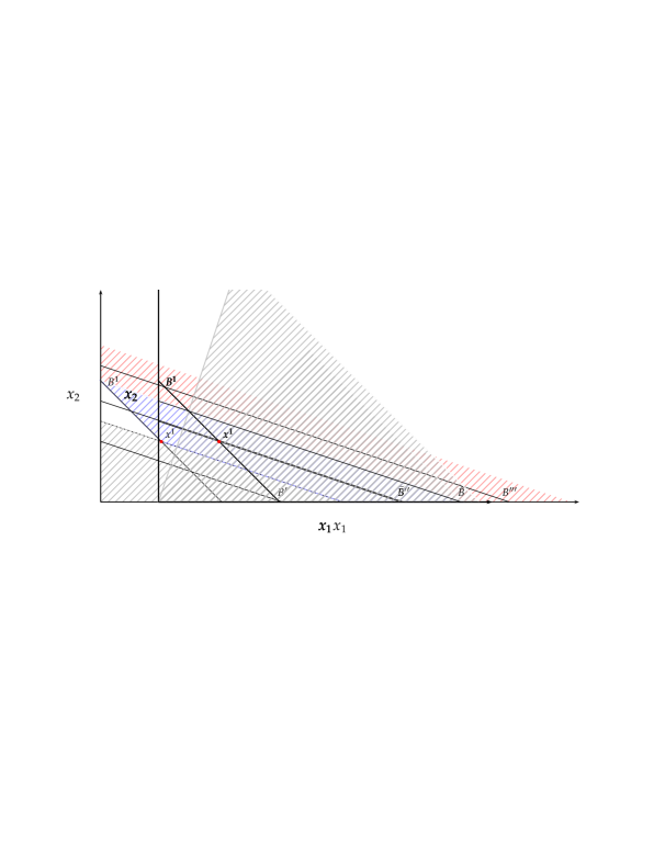
a Counterfactuals using GARP

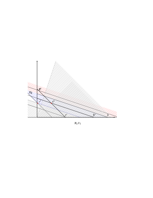
b Counterfactuals using HARP

c Counterfactuals using GAPP

Figure A.1. Counterfactuals with different consumption models

What happens to the predictions of the constrained-maximization model when the utility function is required to be homothetic? It is well known that homothetic utility functions generate demand that is linear in cones. Therefore, for any $x\in\mathbb{R}^{2}_{+}$, the data set $\{(p^{1},x^{1}),(\hat{p},x)\}$ can be rationalized (in the constrained-maximization sense) by a homothetic utility function if and only if $\{(p^{1},x^{1}),(\hat{p},\lambda x)\}$ can also be rationalized in this sense, for any $\lambda>0$. In other words, as in the augmented utility model, the set of predicted demands forms a cone.

The characterization of data sets that are constrained-optimal according to some homothetic preference is given in Varian (1983), where the precise condition is known as the homothetic axiom of revealed preference or HARP, for short. In our simple case, to guarantee that $\{(p^{1},x^{1}),(\hat{p},\lambda x)\}$ satisfies HARP, we set $w=\hat{p}\cdot x^{1}$ and consider the bundles with $\hat{p}\cdot x=w$; the bundles at this expenditure level are depicted by $\widetilde{B}$ in Figure 1b. At this expenditure level, GARP requires that $x$ satisfies $p^{1}\cdot x>p^{1}\cdot x^{1}$ and, for any such $x$, we have $\{(p^{1},x^{1}),(\hat{p},\lambda x)\}$ satisfying HARP; in other words, the set of predicted demands is the cone generated by these bundles of $x$. This cone is depicted by the shaded region in Figure 1b.

In the case of the augmented utility model, recall that if $x$ satisfies $\hat{p}\cdot x=p^{1}\cdot x^{1}=2$, then $\{(p^{1},x^{1}),(\hat{p},x)\}$ satisfies GAPP if and only if it satisfies GARP (see Proposition 1). The budget line with the property that $\hat{p}\cdot x=2$ is $\hat{B}$ in Figure 1c and, in this case, GARP (equivalently, GAPP) requires that $p^{1}\cdot x>p^{1}\cdot x^{1}=2$. The shaded area gives the predicted demands at $\hat{p}$. Notice that the cone in this case contains the cone in Figure 1b, which is consistent with the fact that HARP is a stronger property than GAPP. Furthermore, the predicted demands under GAPP is neither a subset nor a superset of that under GARP, which is again unsurprising given that these two properties are not comparable.

A.1.4. Revealed preferences under GAPP and GARP

Both GARP and GAPP forbids the existences of strict cycles over revealed preference relations: in the case of GARP, the revealed preference relation is defined over bundles and in the case of GAPP it is defined over prices. It is entirely possible for these revealed preference relations to disagree with each other; this occurrence should not be thought of as strange, nor is it an indication that one model is better of worse compared to the other. The two conclusions apply to different objects and either, or both, of them could be interesting to the analyst.

To be precise, suppose that a data $\mathcal{D}=\{(p^{t},x^{t})\}_{t=1}^{T}$ is collected from a consumer who is maximizing an augmented utility function of the form (A.4). Such a data set will obey both GAPP and GARP. It is possible for the price $p^{t}$ to be strictly revealed preferred to $p^{s}$ (whether directly or indirectly) and for the bundle $x^{s}$ to be revealed strictly preferred to $x^{t}$. If this occurs, is the agent better off in observation $t$ or in observation $s$? The fact that $p^{t}$ is revealed strictly preferred to $p^{s}$ means that

$$U(x^{t},-p^{t}\cdot x^{t})>U(x^{s},-p^{s}\cdot x^{s})$$

while the fact that $x^{s}$ is revealed strictly preferred to $x^{t}$ means that

$$\widetilde{U}(x^{t})<\widetilde{U}(x^{s}).$$

In other words, the consumer’s augmented utility is higher in observation $t$ than in observation $s$, even though her sub-utility on the observed bundles is lower in observation $t$; these two phenomena are not mutually exclusive.

Another observation worth making is that it is sometimes possible to conclude that an out-of-sample price $\hat{p}$ is superior to some in-sample price $p^{t_{1}}$ observed in $\mathcal{D}$, even though one has no inkling what the demand will be at $\hat{p}$. Indeed, $\hat{p}$ is revealed preferred to $p^{t_{1}}$ whenever $\hat{p}\cdot x^{t_{1}}\leq p^{t_{1}}\cdot x^{t_{1}}$ (and, more generally, this relation between $\hat{p}$ and some other in-sample price $p^{t}$ can be extended via transitive closure). It follows that at the (unobserved) optimal bundle at $\hat{p}$, which we denote by $\hat{x}$, we must have

$$U(\hat{x},-\hat{p}\cdot\hat{x})\geq U(x^{t_{1}},-\hat{p}\cdot x^{t_{1}})>U(x^{t_{1}},-p^{t_{1}}\cdot x^{t_{1}}).$$

This is true even though, as we know from Section A.1.3, the predicted demand at $\hat{p}$ under the augmented utility model can be an arbitrarily small or large bundle. On the other hand, without knowing the agent’s expenditure level at $\hat{p}$, it is impossible to tell if the sub-utility $\widetilde{U}(\hat{x})$ is greater or lower than $\widetilde{U}(x^{t_{1}})$. Put another way, while GAPP may allow the observer to rank $\hat{p}$ with $p^{t_{1}}$, it is impossible to rank the subutility of the demand bundle at these two observation using GARP, without some information or assumption on the expenditure level at $\hat{p}$.

Example A.6.

Suppose $\mathcal{D}$ consists of two observations,

$$(p^{t_{1}},x^{t_{1}}) = ((2,2),(2,2))\>\mbox{ and}$$

$$(p^{t_{2}},x^{t_{2}}) = ((1,1),(1,1)).$$

It is straightforward to check that this data set can be generated by a consumer maximizing

$$U(x,-e)=\widetilde{U}(x)-f(e),$$

for strictly increasing functions $\widetilde{U}$ and $f$. Clearly, $p^{t_{2}}$ is revealed preferred to $p^{t_{1}}$ and $x^{t_{1}}$ is revealed preferred to $x^{t_{2}}$. In this case, the consumer’s augmented utility is higher at $t_{2}$ compared to $t_{1}$, even though her sub-utility on the observed goods is lower at $t_{2}$ compared to $t_{1}$.

Now suppose the data consists of just the observation $(p^{t_{1}},x^{t_{1}})$. Obviously, we can still conclude that the consumer prefers $\hat{p}=(1,1)$ to $p^{t_{1}}$ and derives greater augmented utility from $\hat{p}$ than from $p^{t_{1}}$. However, nothing can be said about the consumer’s subutility without further information on expenditure. If the expenditure is lower than the expenditure at $t_{1}$, which is 8, then the subutility achieved at $\hat{p}$ must be lower than the subutility of $x^{1}$ and if the expenditure is higher than 8, then the sub-utility achieve must be lower than that of $x^{t_{1}}$.

Appendix A.2 Proof of Proposition 2

(1) We have already shown the ‘only if’ part of this claim, so we need to show the ‘if’ part holds. From the proof of Theorem 1, we know that for a large $M$, it is the case that $p^{t}\succeq_{p}p^{t^{\prime}}$ if and only if $(x^{t},M-p^{t}\cdot x^{t})\succeq_{x}(x^{t^{\prime}},M-p^{t^{\prime}}\cdot x^{t^{\prime}})$ and hence $p^{t}\succeq_{p}^{*}p^{t^{\prime}}$ if and only if $(x^{t},M-p^{t}\cdot x^{t})\succeq_{x}^{*}(x^{t^{\prime}},M-p^{t^{\prime}}\cdot x^{t^{\prime}})$. If $p^{t}\not\succeq_{p}^{*}p^{t^{\prime}}$, then $(x^{t},M-p^{t}\cdot x^{t})\not\succeq_{x}^{*}(x^{t^{\prime}},M-p^{t^{\prime}}\cdot x^{t^{\prime}})$ and hence there is a utility function $\widetilde{U}:\mathbb{R}_{+}^{L+1}\rightarrow\mathbb{R}$ rationalizing the augmented data set $\widetilde{D}$ such that $\widetilde{U}(x^{t},M-p^{t}\cdot x^{t})<\widetilde{U}(x^{t^{\prime}},M-p^{t^{\prime}}\cdot x^{t^{\prime}})$ (see Remark 2 in Section A.1.1). This in turn implies that the augmented utility function $U$ (as defined by (5)), has the property that $U(x^{t},-p^{t}\cdot x^{t})<U(x^{t^{\prime}},-p^{t^{\prime}}\cdot x^{t^{\prime}})$ or, equivalently, $V(p^{t})<V(p^{t^{\prime}})$.

(2) Given part (1), we need only show that if $p^{t}\succeq_{p}^{*}p^{t^{\prime}}$ but $p^{t}\not\succ_{p}^{*}p^{t^{\prime}}$, then there is some augmented utility function $U$ such that $U(x^{t},-p^{t}\cdot x^{t})=U(x^{t^{\prime}},-p^{t^{\prime}}\cdot x^{t^{\prime}})$. To see that this holds, note that if $p^{t}\succeq_{p}^{*}p^{t^{\prime}}$ but $p^{t}\not\succ_{p}^{*}p^{t^{\prime}}$, then $(x^{t},M-p^{t}\cdot x^{t})\succeq^{*}_{x}(x^{t^{\prime}},M-p^{t^{\prime}}\cdot x^{t^{\prime}})$ but $(x^{t},M-p^{t}\cdot x^{t})\not\succ^{*}_{x}(x^{t^{\prime}},M-p^{t^{\prime}}\cdot x^{t^{\prime}})$. In this case there is a utility function $\widetilde{U}:\mathbb{R}_{+}^{L+1}\rightarrow\mathbb{R}$ rationalizing the augmented data set $\widetilde{D}$ such that $\widetilde{U}(x^{t},M-p^{t}\cdot x^{t})=\widetilde{U}(x^{t^{\prime}},M-p^{t^{\prime}}\cdot x^{t^{\prime}})$. This in turn implies that the augmented utility function $U$ (as defined by (5)) satisfies $U(x^{t},-p^{t}\cdot x^{t})=U(x^{t^{\prime}},-p^{t^{\prime}}\cdot x^{t^{\prime}})$ and so $V(p^{t})=V(p^{t^{\prime}})$. $\blacksquare$

Appendix A.3 Price indices to deflate nominal expenditure

In this section, we build on the discussion in Section 3.5. Suppose that, at observation $t$, the consumer chooses $(x^{t},y^{t})$ to maximize $\widetilde{U}(x,y)$, subject to $p^{t}\cdot x^{t}+q^{t}\cdot y^{t}\leq M^{t}$. We are interested in the conditions under which there is an index $k^{t}$, depending on the prices of the outside goods, such that the deflated data $\{(p^{t}/k^{t},x^{t})\}_{t=1}^{T}$ obeys GAPP (and hence can be rationalized as maximizing an augmented utility function). In the main paper, we explained that this holds if prices of the outside goods move up and down proportionately (so there is no change to their prices relative to each other). When relative prices are allowed to change, it is still possible to obtain a deflator $k^{t}$ guaranteeing that $\{(p^{t}/k^{t},x^{t})\}_{t=1}^{T}$ obeys GAPP, but stronger assumptions will have to be imposed on the utility function $\widetilde{U}$. We outline a set of sufficient conditions for this to hold.

Suppose that the outside goods are weakly separable from the observed goods, so the overall utility function has the form $\widetilde{U}(x,\tilde{u}(y))$, where $\tilde{u}(y)$ is the sub-utility of the bundle $y$ of outside goods. Furthermore, we assume that $\tilde{u}$ has an indirect utility $\tilde{v}$ of the following form:

$$\tilde{v}(q,m)=h\left(\frac{m}{f(q)}+b(q),g_{1}(q),g_{2}(q),\ldots,g_{N}(q)\right)$$

where $f$, $b$, $g_{1},\ldots,g_{N}$ are all real-valued functions of the prices $q$ of the outside goods, and $m$ is the expenditure devoted to those goods. This formulation covers a number of standard functional forms used in empirical analysis. If $\tilde{v}(q,m)=m/f(q)$ where $f$ is one-homogeneous then the preference it generates is homothetic; if $\tilde{v}(q,m)=(m/f(q))+b(q)$, where $b$ is zero-homogeneous, then we obtain the Gorman polar form (see Gorman (1961)). Another example is the form

$$\ln\tilde{v}(q,m)=\left\{\left[\frac{\ln m-\ln f(q)}{g_{1}(q)}\right]^{-1}+g_{2}(q)\right\}^{-1}$$ (A.5)

where $g_{1}$ and $g_{2}$ are zero-homogeneous functions. If $g_{2}\equiv 0$, the form (A.5) generates the Price Invariant Generalized Logarithmic (PIGLOG) demand system Muellbauer (1976); if further functional form restrictions are imposed on $f$ and $g_{1}$, we obtain the Almost Ideal Demand System (AIDS) of Deaton and Muellbauer (1980). The Quadratic Almost Ideal Demand System (QUAIDS) is a generalization of AIDS that has greater flexibility to model empirically relevant Engel curves (see Banks, Blundell, and Lewbel (1997)); it is a special case of (A.5) with functional form restrictions on $f$, $g_{1}$, and $g_{2}$.

We assume that the consumer’s total wealth $M^{t}$ varies with $t$ in such a way that, should the consumer devote all of this wealth to the unobserved goods, then her utility is constant. This captures the idea that the consumer’s real wealth (as measured by the indirect utility function $v$) is unchanged across observations. While we permit prices of the unobserved goods to change, we require that they change in such a way that $g_{1}(q^{t})$, $g_{2}(q^{t}),\ldots,g_{N}(q^{t})$ remain constant at $\bar{g}_{1},\bar{g}_{2}\ldots,\bar{g}_{N}$ (respectively) for all $t$. Given the form of $\tilde{v}$, this implies that $(M^{t}/f(q^{t}))+b(q^{t})$ is constant for all $t$; let this constant be $C$. Thus we can think of the consumer as choosing $(x,c)$ to maximize $\widetilde{U}(x,\tilde{v}(c,\bar{g}_{1},\bar{g}_{2},\ldots,\bar{g}_{N}))$ subject to $p^{t}\cdot x+(c-b(q^{t}))f(q^{t})\leq(C-b(q^{t}))f(q^{t})$. This inequality can be written as

$$\frac{p^{t}\cdot x}{f(q^{t})}+c\leq C.$$

It follows that the data set $\{(p^{t}/f(q^{t}),x^{t})\}_{t=1}^{T}$ will obey GAPP.

Appendix A.4 Nonlinear pricing, the rationality index, and related topics

In this section, we formulate and prove a rationalization result that allows for both imperfect rationalization and nonlinear pricing. This result generalizes Theorem 2 and Theorem 1 by allowing for imperfect rationality. We explain how this result is crucial in helping us to calculate the rationality index (introduced in Section 3.4) and other variations on that index that provide a measure of departures from exact rationality. We also use this result to show that the bounds on the compensating and equivalent variations obtained in Section 3.3 are tight.

A.4.1. $\overline{\vartheta}$-rationalization

We are in the setting of Section 4. The consumer chooses her consumption from the space $X\subseteq\mathbb{R}_{+}^{L}$. A price system is a map $\psi:X\to\mathbb{R}_{+}$, where $\psi(x)$ is the cost of purchasing $x\in X$. Let $\overline{\vartheta}=(\vartheta^{1},\vartheta^{2},\dots,\vartheta^{T})\in(0,1]^{T}$. An augmented utility function $U:X\times\mathbb{R}_{+}\to\mathbb{R}$ provides a $\overline{\vartheta}$-rationalization of a data set $\mathcal{D}=\{(\psi^{t},x^{t})\}_{t=1}^{T}$ if, at each observation $t$,

$$U(x^{t},-\psi^{t}(x^{t}))\geq U(x,-(\vartheta^{t})^{-1}\psi^{t}(x))\>\mbox{ for all $x\in X$.}$$

Note that this definition of $\overline{\vartheta}$-rationalization generalizes the notion introduced in Section 3.4, which can be thought of as the special case where $\vartheta^{t}=\vartheta^{t^{\prime}}$ for all $t$, $t^{\prime}\in T$. The context here is also more general since we allow for nonlinear pricing (as introduced in Section 4). Obviously, if a data set can be exactly rationalized then it is $\overline{\vartheta}$-rationalized with $\overline{\vartheta}=(1,1,\ldots,1)$; note also that if a data set can be $\overline{\vartheta}$-rationalized then it can also be $\overline{\vartheta}^{\prime}$-rationalized for $\overline{\vartheta}^{\prime}<\overline{\vartheta}$. A consumer whose observations cannot be exactly rationalized but can be $\overline{\vartheta}$-rationalized for some $\overline{\vartheta}<(1,1,\ldots,1)$ exhibits limited rationality in the sense discussed in Section 3.4.

The calculation of the rationality index hinges on our ability to ascertain whether a data set $\mathcal{D}$ has a $\overline{\vartheta}$-rationalization for a given $\overline{\vartheta}$. It is possible to characterize those data sets that can be $\overline{\vartheta}$-rationalized using a modified version of the GAPP test, as we now explain.

Let $\overline{\vartheta}\in(0,1]^{T}$. Define the relations $\succeq_{p,\overline{\vartheta}}$ and $\succ_{p,\overline{\vartheta}}$ in the following way:

$\psi^{t^{\prime}}\succeq_{p,\overline{\vartheta}}\psi^{t}$ if $\psi^{t^{\prime}}(x^{t})\leq\vartheta^{t^{\prime}}\psi^{t}(x^{t})$ and $\psi^{t^{\prime}}\succ_{p,\overline{\vartheta}}\psi^{t}$ if $\psi^{t^{\prime}}(x^{t})<\vartheta^{t^{\prime}}\psi^{t}(x^{t})$.

Denote the transitive closure of $\succeq_{p,\overline{\vartheta}}$ by $\succeq^{*}_{p,\overline{\vartheta}}$. Obviously these definitions generalize the ones given for revealed preference relations over prices provided in Section 4.

The data set $\mathcal{D}$ obeys $\overline{\vartheta}$-GAPP if

there do not exist observations $t,t^{\prime}\in T$ such that $\psi^{t^{\prime}}\succeq^{*}_{p,\overline{\vartheta}}\psi^{t}$ and $\psi^{t}\succ_{p,\overline{\vartheta}}\psi^{t^{\prime}}$.

The next result states that $\overline{\vartheta}$-GAPP characterizes $\overline{\vartheta}$-rationalization.

Theorem A.4.1

A data set $\mathcal{D}=\{(\psi^{t},x^{t})\}_{t=1}^{T}$ can be $\overline{\vartheta}$-rationalized by an augmented utility function for some $\overline{\vartheta}\in(0,1]^{T}$ if and only if it satisfies $\overline{\vartheta}$-GAPP.

Remark 1.  This theorem states, in particular, that $\mathcal{D}=\{(\psi^{t},x^{t})\}_{t=1}^{T}$ can be rationalized by an augmented utility function if and only if it satisfies GAPP, which corresponds to the special case where $\overline{\vartheta}=(1,1,\ldots,1)$. So it covers the first claim in Theorem 2 (the part before “Furthermore,…”) and also the equivalence of statements (1) and (2) in Theorem 1. For the proof of the second claim in Theorem 2 see the end of this subsection. Unlike the proof we gave of Theorem 1 in the main body of the paper, our proof of Theorem A.4.1 does not appeal to Afriat’s Theorem, though it is clearly inspired by it. In particular, we show that $\overline{\vartheta}$-GAPP implies that there is a solution to a system of linear inequalities (see Lemma A.1 below), analogous to the so-called Afriat inequalities usually derived in the proof of Afriat’s Theorem and then use those inequalities to explicitly construct a piecewise linear augmented utility function that rationalizes the data.

Remark 2.  Note that checking whether or not $\overline{\vartheta}$-GAPP holds for a given $\overline{\vartheta}$ is computationally undemanding: the relations $\succeq_{p,\overline{\vartheta}}$ and $\succ_{p,\overline{\vartheta}}$ can be easily constructed; once this has been obtained, we can apply Warshall’s algorithm to compute the transitive closure of the revealed preference relations and then check for violations of $\overline{\vartheta}$-GAPP.

Remark 3.  Suppose we impose the mild restriction that every bundle that is an observed choice has a strictly positive value under any of the other price observation, that is, $\psi^{t^{\prime}}(x^{t})>0$ whenever $\psi^{t^{\prime}}\neq\psi^{t}$. Then we can choose sufficiently small $\vartheta>0$ so that $\psi^{t^{\prime}}(x^{t})>\vartheta\psi^{t}(x^{t})$ whenever $\psi^{t^{\prime}}\neq\psi^{t}$. If we let $\overline{\vartheta}=(\vartheta,\ldots,\vartheta)$, then $\mathcal{D}$ must obey $\overline{\vartheta}$-GAPP simply because the relation $\succ_{p,\overline{\vartheta}}$ is empty. Thus every data set is $\overline{\vartheta}$-rationalizable for $\overline{\vartheta}$ sufficiently close to zero.

Proof of Theorem A.4.1.  Suppose $\mathcal{D}$ can be $\overline{\vartheta}$-rationalized by an augmented utility function for some $\overline{\vartheta}\in(0,1]^{T}$. In that case, if $\psi^{t^{\prime}}\succeq_{p,\overline{\vartheta}}\psi^{t}$, then $\psi^{t^{\prime}}(x^{t})\leq\vartheta^{t^{\prime}}\psi^{t}(x^{t})$ and so

$$U(x^{t^{\prime}},-\psi^{t^{\prime}}(x^{t^{\prime}}))\geq U(x^{t},-(\vartheta^{t^{\prime}})^{-1}\psi^{t^{\prime}}(x^{t}))\geq U(x^{t},-\psi^{t}(x^{t})),$$ (A.6)

where the first inequality follows from the (imperfect) optimality of $x^{t^{\prime}}$ and the second from the property that $U$ is strictly decreasing in expenditure. It follows that if $\psi^{t^{\prime}}\succeq^{*}_{p,\overline{\vartheta}}\psi^{t}$, then $U(x^{t^{\prime}},-\psi^{t^{\prime}}(x^{t^{\prime}}))\geq U(x^{t},-\psi^{t}(x^{t}))$. Similarly, if $\psi^{t^{\prime}}\succ_{p,\overline{\vartheta}}\psi^{t}$, then $\psi^{t^{\prime}}(x^{t})<\vartheta^{t^{\prime}}\psi^{t}(x^{t})$ and we obtain $U(x^{t^{\prime}},-\psi^{t^{\prime}}(x^{t^{\prime}}))>U(x^{t},-\psi^{t}(x^{t}))$ since the second inequality in (A.6) will now be strict. It is then clear that we cannot simultaneously have $\psi^{t^{\prime}}\succeq^{*}_{p,\overline{\vartheta}}\psi^{t}$, and $\psi^{t}\succ_{p,\overline{\vartheta}}\psi^{t^{\prime}}$, which establishes $\overline{\vartheta}$-GAPP.

Conversely, suppose that $\mathcal{D}$ obeys $\overline{\vartheta}$-GAPP. Then there is a complete preorder $\succsim$ defined on the set $\{p^{t}\}_{t\in T}$ that extends $\succeq_{p,\overline{\vartheta}}$ and $\succ_{p,\overline{\vartheta}}$ in the sense that such $\psi^{t^{\prime}}\succsim\psi^{t}$ if $\psi^{t^{\prime}}\succeq^{*}_{p,\overline{\vartheta}}\psi^{t}$ and $\psi^{t^{\prime}}\succ\psi^{t}$ if $\psi^{t^{\prime}}\succ_{p,\overline{\vartheta}}\psi^{t}$, where $\succ$ is the asymmetric part of $\succsim$. We first prove the following lemma.

Lemma A.1

Suppose $\mathcal{D}$ obeys $\overline{\vartheta}$-GAPP and let $\succsim$ be a complete preorder that extends $\succeq_{p,\overline{\vartheta}}$ and $\succ_{p,\overline{\vartheta}}$. Then there are numbers $\phi^{t}$ and $\lambda^{t}>0$ (for $t=1,2,\ldots,T$) with the following properties:

• $\phi^{t^{\prime}}>\phi^{t}$ if $\psi^{t^{\prime}}\succ\psi^{t}$;

• $\phi^{t^{\prime}}=\phi^{t}$ if $\psi^{t^{\prime}}\sim\psi^{t}$; and

• $\phi^{t^{\prime}}\leq\phi^{t}+\lambda^{t}(\psi^{t}(x^{t^{\prime}})-\vartheta^{t}\psi^{t^{\prime}}(x^{t^{\prime}}))$ for all $t\neq t^{\prime}$.

Proof.  Let $z^{ij}=\psi^{i}(x^{j})-\vartheta^{i}\psi^{j}(x^{j})$ for $i,\,j\in T$. Note that, for $i\neq j$, $z^{ij}<0$ implies that $\psi^{i}\succ\psi^{j}$ and $z^{ij}\leq 0$ implies that $\psi^{i}\succsim\psi^{j}$. We shall explicitly construct $\phi^{t}$ and $\lambda^{t}>0$ that satisfy the required conditions. With no loss of generality, suppose that $\psi^{t+1}\succsim\psi^{t}$ for $t=1,2,\ldots,T-1$.

First, choose $\phi^{1}$ to be any number and $\lambda^{1}$ to be any strictly positive number. Suppose $\psi^{2}\succ\psi^{1}$. Then $\min_{j>1}z^{1j}>0$, because if $z^{1j^{\prime}}=\psi^{1}(x^{j^{\prime}})-\vartheta^{1}\psi^{j^{\prime}}(x^{j^{\prime}})\leq 0$ for some $j^{\prime}>1$, then $\psi^{1}\succsim\psi^{j^{\prime}}$, which is a contradiction. So there is $\phi^{2}$ such that

$$\phi^{1}<\phi^{2}<\min_{j>1}\{\phi^{1}+\lambda^{1}z^{1j}\}.$$ (A.7)

If $\psi^{2}\sim\psi^{1}$ then $\min_{j>1}z^{1j}\geq 0$ because if $z^{1j^{\prime}}=\psi^{1}(x^{j^{\prime}})-\vartheta\psi^{j^{\prime}}(x^{j^{\prime}})<0$ for some $j^{\prime}>1$, then $\psi^{1}\succ\psi^{j^{\prime}}$, which is a contradiction. Setting $\phi^{2}=\phi^{1}$, we obtain

$$\phi^{1}=\phi^{2}\leq\min_{j>1}\{\phi^{1}+\lambda^{1}z^{1j}\}.$$ (A.8)

We claim that there is $\lambda^{2}>0$ such that

$$\phi^{1}\leq\phi^{2}+\lambda^{2}z^{21}.$$

Clearly this inequality holds if $z^{21}\geq 0$. If $z^{21}=\psi^{2}(x^{1})-\vartheta^{2}\psi^{1}(x^{1})<0$, then $\psi^{2}\succ\psi^{1}$; this implies that $\phi^{1}<\phi^{2}$ and thus the inequality holds for $\lambda^{2}$ sufficiently small.

We now go on to choose $\phi^{3}$ and $\lambda^{3}$. Since $\psi^{j}\succsim\psi^{i}$ for all $j>2$ and $i=1,2$, we obtain $z^{ij}\geq 0$. Consider two cases: when $\psi^{3}\succ\psi^{2}\succsim\psi^{1}$ and $\psi^{3}\sim\psi^{2}\succsim\psi^{1}$. In the former case, both $\min_{j>2}z^{1j}>0$ and $\min_{j>2}z^{2j}>0$. Therefore

$$\phi^{2}<\min_{j>2}\{\phi^{2}+\lambda^{2}z^{2j}\}.$$

If $\phi^{2}=\phi^{1}$, obviously we also have

$$\phi^{2}<\min_{j>2}\{\phi^{1}+\lambda^{1}z^{1j}\}\mbox{;}$$

this inequality also holds if $\phi^{2}>\phi^{1}$ since in that case (A.7) holds. It follows that we can find $\phi^{3}$ such that

$$\phi^{2}<\phi^{3}<\min\left\{\min_{j>2}\{\phi^{1}+\lambda^{1}z^{1j}\},\min_{j>2}\{\phi^{2}+\lambda^{2}z^{2j}\}\right\}.$$

We turn to the case where $\psi^{3}\sim\psi^{2}\succsim\psi^{1}$. It follows from (A.7) and (A.8) that $\phi^{2}\leq\min_{j>2}\{\phi^{1}+\lambda^{1}z^{2j}\}$. We also know that $z^{2j}\geq 0$ for all $j>2$. Therefore, we can choose $\phi^{3}$ such that

$$\phi^{2}=\phi^{3}\leq\min\left\{\min_{j>2}\{\phi^{1}+\lambda^{1}z^{1j}\},\min_{j>2}\{\phi^{2}+\lambda^{2}z^{2j}\}\right\}.$$

Now choose $\lambda^{3}>0$ sufficiently small so that

$$\phi^{i}\leq\phi^{3}+\lambda^{3}z^{3i}\>\mbox{ for $i=1,2$.}$$

Clearly that this inequality holds for any $\lambda^{3}>0$ if $z^{3i}\geq 0$. If $z^{3i}<0$ then $\psi^{3}\succ\psi^{i}$, in which case $\phi^{3}>\phi^{i}$ and the inequality will be satisfied for $\lambda^{3}$ sufficiently small.

Repeating this argument, we choose $\phi^{t}$ (for $t\leq T-1$) such that if $\psi^{t}\succ\psi^{t-1}$ then

$$\phi^{t-1}<\phi^{t}<\min_{s\leq t-1}\left\{\min_{j>t-1}\{\phi^{s}+\lambda^{s}z^{sj}\}\right\}$$ (A.9)

and if $\psi^{t}\sim\psi^{t-1}$ then

$$\phi^{t-1}=\phi^{t}\leq\min_{s\leq t-1}\left\{\min_{j>t-1}\{\phi^{s}+\lambda^{s}z^{sj}\}\right\}\mbox{;}$$ (A.10)

and $\lambda^{t}>0$ (for $t=2,3,\ldots,T$) such that

$$\phi^{i}\leq\phi^{t}+\lambda^{t}z^{ti}\>\mbox{ for $i\leq t-1$.}$$ (A.11)

For a fixed $t^{\prime}$, (A.9) and (A.10) guarantee that $\phi^{t^{\prime}}\leq\phi^{t}+\lambda^{t}z^{tt^{\prime}}$ for $t<t^{\prime}$ while (A.11) guarantees that this inequality holds for $t>t^{\prime}$. So we have found $\lambda^{t}$ and $\phi^{t}$ to obey condition (c), while the first two conditions hold by construction. $\blacksquare$

We now return to the proof that (2) implies (3). Let $\succsim$ be a complete preorder that extends $\succeq_{p,\overline{\vartheta}}$ and $\succ_{p,\overline{\vartheta}}$ and let the numbers $\phi^{t}$ and $\lambda^{t}>0$ (for $t=1,2,\ldots,T$) satisfy properties (a) – (c) in Lemma A.1. Define the function $U:X\times\mathbb{R}_{-}\to\mathbb{R}$ by

$$U(x,-e)=\min_{t\in T}\{\phi^{t}+\lambda^{t}(\psi^{t}(x)-\vartheta^{t}e)\}.$$ (A.12)

This function is an augmented utility function since it is strictly increasing in the last argument. We claim that this function also satisfies the property that, at each $t\in T$,

$$U(x^{t},-\psi^{t}(x^{t}))\geq U(x,-(\vartheta^{t})^{-1}\psi^{t}(x))\>\mbox{ for all $x\in X$.}$$

Indeed, at a given observation $s$, for any $t\neq s$, we have $\phi^{t}+\lambda^{t}(\psi^{t}(x^{s})-\vartheta^{t}\psi^{s}(x^{s}))\geq\phi^{s}$ by condition (c); furthermore, $\phi^{s}+\lambda^{s}(\psi^{s}(x^{s})-\vartheta^{s}\psi^{s}(x^{s}))\geq\phi^{s}$ since $\lambda^{s}>0$ and $\vartheta^{s}\in(0,1]$. Therefore, $U(x^{s},-\psi^{s}(x^{s}))\geq\phi^{s}$. On the other hand, by the definition of $U$,

$$U(x,-(\vartheta^{s})^{-1}\psi^{s}(x))\leq\phi^{s}+\lambda^{s}(\psi^{s}(x)-\psi^{s}(x))\leq\phi^{s}.$$

So $U(x^{s},-\psi^{s}(x^{s}))\geq U(x,-\vartheta^{-1}\psi^{s}(x))$ for all $x$. $\blacksquare$

The augmented utility function $U$ at the price system $\psi$ induces an indirect utility given by $V(\psi)=\max_{x\in X}U(x,-\psi(x))$. In the case where GAPP holds and exact rationalization is possible, one could also choose the rationalizing utility function $U$ so that its indirect utility $V$ agrees with any ordering over $\{\psi^{t}\}_{t=1}^{T}$ that is consistent with the revealed preference relations. (Note that this feature is also present in Afriat’s Theorem; see Remark 2 in Section A.1.1.) The following result is used in Section A.5.

Theorem A.4.2

Suppose the data set $\mathcal{D}=\{(\psi^{t},x^{t})\}_{t=1}^{T}$ obeys GAPP and let $\succsim$ be a complete preorder on $\{\psi^{t}\}_{t=1}^{T}$ that extends $\succeq_{p}$ and $\succ_{p}$. Then there is an augmented utility function $U:X\times\mathbb{R}_{-}\to\mathbb{R}$ that rationalizes $\mathcal{D}$ such that $V(\psi^{t^{\prime}})=V(\psi^{t})$ if $\psi^{t^{\prime}}\sim\psi^{t}$ and $V(\psi^{t})>V(\psi^{t})$ if $\psi^{t^{\prime}}\succ\psi^{t}$ (where $\sim$ and $\succ$ are the symmetric and asymmetric parts of $\succsim$).

Proof.  From the proof of Theorem A.4.1, we know that $U(x,-e)$ as given by (A.12) (with $\theta^{t}=1$ for all $t$) rationalizes $\mathcal{D}$. We can then conclude that $V(\psi^{t})=U(x^{t},-\psi(x^{t}))=\phi^{t}$ because $\phi^{t}\leq\phi^{t^{\prime}}+\lambda^{t^{\prime}}(\psi^{t^{\prime}}(x^{t})-\psi^{t}(x^{t}))$ from part (c) of Lemma A.1. Finally, $V$ satisfies the required properties because of (a) and (b) in Lemma A.1. $\blacksquare$

We end this subsection with the proof of Theorem 2; this result is obtained as a corollary of Theorem A.4.1.

Proof of Theorem 2.  Choosing $\overline{\vartheta}=(1,1,\ldots,1)$, Theorem A.4.1 states, in particular, that $\mathcal{D}=\{(\psi^{t},x^{t})\}_{t=1}^{T}$ can be rationalized by an augmented utility function if and only if it satisfies GAPP. It remains for us to show that, under assumptions (i), (ii), and (iii), this utility function could be extended to one defined on a closed set $Y$ containing $X$ and that is increasing in $x_{K}$. We know from the proof of Theorem 2 that the function $U:X\to\mathbb{R}$ given by

$$U(x,-e)=\min_{t\in T}\{\phi^{t}+\lambda^{t}(\psi^{t}(x)-e)\}.$$

rationalizes the data (see A.12). It suffices to show that each function $\psi^{t}$, which is defined on $X$ could be extended to a continuous function on $Y$ that is strictly increasing in $x_{K}$, in which case we could correspondingly extend $U$ and the extension would be continuous and strictly increasing in $x_{K}$ (since $\lambda^{T}>0$).

That $\psi^{t}$ admits such an extension is guaranteed by (i), (ii), and (iii). A quick way of arriving at this conclusion is to appeal to Levin’s Theorem, which is a version of Szpilrajn’s Theorem for closed preorders (see Nishimura, Ok, and Quah (2017) for a proof of Levin’s Theorem). Since $\psi^{t}$ is continuous, it induces a closed preorder $\succsim^{\prime}$ on $X$ and therefore also on $Y$. For $K\subset L$, let $\geq_{K}$ be the partial order on $Y$ such that, for $x^{\prime}$ and $x$ in $\mathbb{R}^{L}$, we have $x^{\prime}\geq_{K}x$ if $x^{\prime}_{i}\geq x_{i}$ for all $i\in K$ and $x_{i}^{\prime}=x_{i}$ for $i\notin K$. It is straightforward to check that, for any number $M$, the set

$$\{x\in Y:\mbox{there is $\tilde{x}\in X$ with $\tilde{x}\geq_{K}x$ and $M\geq\psi^{t}(\tilde{x})$}\}$$

is a compact set in $Y$. (Recall that $Y$ is closed, contains $X$, and is contained in $\mathbb{R}^{L}_{+}$.) Using this property, one could check that $\succsim^{\prime\prime}$, defined as the transitive closure of $\succsim^{\prime}$ and $\geq_{K}$, is also a closed prorder on $Y$. Levin’s Theorem then guarantees that there is a complete and closed preorder $\succsim$ on $Y$ that extends $\succsim^{\prime\prime}$ and has a continuous representation $V:Y\to\mathbb{R}$. In particular, $V$ must be strictly increasing in $x_{K}$ and satisfies the following property: $V(x^{\prime})\geq(>)\,V(x)$ if $\psi^{t}(x^{\prime})\geq(>)\,\psi^{t}(x)$, for $x^{\prime}$, $x\in X$. Furthermore, our assumptions guarantee that that $\{V(x):x\in X\}\subseteq\mathbb{R}$ is a closed set. These properties guarantee that we could choose a strictly increasing transformation $h$ defined on the range of $V$, i.e., the set $\{V(x):x\in Y\}$, so that $h(V(x))=\psi^{t}(x)$ for all $x\in X$. Therefore the function $h\circ V:Y\to\mathbb{R}$ is a continuous extension of $\psi^{t}:X\to\mathbb{R}$ that is strictly increasing in $x_{K}$. $\blacksquare$

A.4.2. Rationality indices and their computation

Given a data set $\mathcal{D}=\{(\psi^{t},x^{t})\}_{t=1}^{T}$, we know that it admits a $(\vartheta,\vartheta,\ldots,\vartheta)$-rationalization for some $\vartheta>0$ (see Remark 3 following Theorem A.4.1). This guarantees that the rationality index, given by

$$\vartheta^{*}=\sup\{\vartheta\in(0,1]:\mbox{$\mathcal{D}$ has a $(\vartheta,\vartheta,\ldots,\vartheta)$-rationalization}\},$$

is well-defined. Note that this definition generalizes the definition provided in Section 3.4 of the main paper, which applies to the linear price environment. A data set that can be rationalized exactly has a rationality index of 1 and we could use the closeness of $\vartheta^{*}$ to 1 as a measure of the data set’s closeness to exactly rationality.

Given the characterization of $\overline{\vartheta}$-rationality stated in Theorem A.4.1, we also have

$$\vartheta^{*}=\sup\{\vartheta\in(0,1]:\mbox{$\mathcal{D}$ satisfies $(\vartheta,\vartheta,\ldots,\vartheta)$-GAPP}\}.$$ (A.13)

This identity provides us with a practical way of calculating $\vartheta^{*}$. Indeed, $\vartheta^{*}$ can be obtained through a binary search algorithm that works as follows. We first set the lower and upper bounds on $\vartheta^{*}$ to be $\vartheta^{L}=0$ and $\vartheta^{H}=1$. We then check (by checking $\overline{\vartheta}$-GAPP) whether the data set passes or fails the test at $\vartheta=(\vartheta^{L}+\vartheta^{H})/2$ (to be precise, at $\overline{\vartheta}=(\vartheta,\vartheta,\ldots,\vartheta)$); if it passes the test, then we update both $\vartheta^{*}$ and its lower bound to $(\vartheta^{L}+\vartheta^{H})/2$; if it fails the test, then we update $\vartheta^{*}$ to $\vartheta^{L}$ and the upper bound on $\vartheta^{*}$ to $(\vartheta^{L}+\vartheta^{H})/2$. We then repeat the procedure, selecting and testing the new midpoint of the updated lower and upper bounds. The algorithm terminates when the lower and upper bounds are sufficiently close.

There are other plausible variations on the rationality index, based on the way one aggregates $\vartheta^{t}$ across observations. Let $F:(0,1]^{T}\to\mathbb{R}_{+}$ be any weakly increasing function taking nonnegative values such that $F(1,1,\ldots,1)=1$. We can then construct a generalized rationality index

$$F^{*}=\sup\{F(\overline{\vartheta}):\mbox{$\mathcal{D}$ has a $\overline{\vartheta}$-rationalization}\}.$$

The rationality index $\vartheta^{*}$ corresponds to the case where $F$ is defined by

$$F(\overline{\vartheta})=\min\{\vartheta^{1},\vartheta^{2},\ldots,\vartheta^{T}\}.$$

As an alternative to this, one could choose

$$F(\overline{\vartheta})=1-\sqrt{(1-\vartheta^{1})^{2}+(1-\vartheta^{2})^{2}+\ldots+(1-\vartheta^{T})^{2}}\,,$$

which leads to a measure of rationality based on the sum of square differences from the case of exact rationality (where $\overline{\vartheta}=(1,1,\ldots,1)$).

Computing these generalized rationality indices can be more demanding than computing the (basic) rationality index $\vartheta^{*}$ since in searching for those values of $\overline{\vartheta}$ that $\overline{\vartheta}$-rationalizes the data and maximizes $F(\overline{\vartheta})$, we would not in general be able to confine ourselves to the the case where $\vartheta^{t}=\vartheta^{t^{\prime}}$ for all $t$, $t^{\prime}$. In the literature on measuring GARP violations, there are indices, such as the one proposed by Varian (1990), that involve solving a maximization problem with the same mathematical structure. (In that case the problem is to find the best way to break up revealed preference cycles over consumption bundles rather than over price vectors.) Algorithms that have been devised to compute Varian’s index (see Halevy, Persitz, and Zrill (2018) and Polisson, Quah, and Renou (2020)) can also be used to compute $F^{*}$.

A.4.3. $\overline{\vartheta}$-GAPP and $\overline{\vartheta}$-GARP

We confine our discussion to the environment where prices are linear, so the data set has the form $\mathcal{D}=\{(p^{t},x^{t})\}_{t=1}^{T}$. Let $\overline{\vartheta}\in(0,1]^{T}$. We say that a utility function $\widetilde{U}:\mathbb{R}^{L}_{+}\to\mathbb{R}$ $\overline{\vartheta}$-rationalizes $\mathcal{D}$ in the sense of Afriat if $\widetilde{U}(x^{t})\geq\widetilde{U}(x)$ for all $x\in B^{t}_{\overline{\vartheta}}$, where

$$B^{t}_{\overline{\vartheta}}=\{x\in\mathbb{R}^{L}_{+}:p^{t}\cdot x\leq\vartheta^{t}p^{t}\cdot x^{t}\}.$$

$\overline{\vartheta}$-rationalization in this sense admits a characterization similar to the one we gave for $\overline{\vartheta}$-rationalization in the augmented utility model.

Define the relations $\succeq_{x,\overline{\vartheta}}$ and $\succ_{x,\overline{\vartheta}}$ on the set $\{x^{t}\}_{t=1}^{T}$ in the following way:

$x^{t^{\prime}}\succeq_{x,\vartheta}x^{t}$ if $p^{t^{\prime}}\cdot x^{t}\leq\vartheta^{t^{\prime}}p^{t^{\prime}}\cdot x^{t^{\prime}}$ and $x^{t^{\prime}}\succ_{x,\vartheta}x^{t}$ if $p^{t^{\prime}}\cdot x^{t}<\vartheta^{t^{\prime}}p^{t^{\prime}}\cdot x^{t^{\prime}}$

Denote the transitive closure of $\succeq_{x,\overline{\vartheta}}$ by $\succeq^{*}_{x,\overline{\vartheta}}$. Obviously these definitions generalize the ones given for the revealed preference relations over bundles (see Section 2.2 of the main paper). With these definitions in place, we can also generalize the definition of GARP. We say that the data set $\mathcal{D}$ obeys $\overline{\vartheta}$-GARP if

there do not exist observations $t,t^{\prime}\in T$ such that $x^{t^{\prime}}\succeq^{*}_{x,\overline{\vartheta}}x^{t}$ and $x^{t}\succ_{x,\overline{\vartheta}}x^{t^{\prime}}$.

It is straightforward to show that $\overline{\vartheta}$-GARP is necessary for the $\overline{\vartheta}$-rationalization of $\mathcal{D}$ (in the sense of Afriat) by a locally nonsatiated utility function $\widetilde{U}:\mathbb{R}^{L}_{+}\to\mathbb{R}$. It is also known (see Halevy, Persitz, and Zrill (2018)) that $\overline{\vartheta}$-GARP is sufficient to guarantee the $\overline{\vartheta}$-rationalization of $\mathcal{D}$ (in Afriat’s sense) by a continuous, strictly increasing and concave utility function $\widetilde{U}:\mathbb{R}^{L}_{+}\to\mathbb{R}$. By definition, the critical cost efficiency index $c^{*}$ satisfies

$$c^{*}=\sup\{\vartheta\in(0,1]:\mbox{$\mathcal{D}$ has a $(\vartheta,\vartheta,\ldots,\vartheta)$-rationalization in the sense of Afriat}\}$$

and since $\overline{\vartheta}$-rationalization in Afriat’s sense can be characterized by $\overline{\vartheta}$-GARP, we obtain

$$c^{*}=\sup\{\vartheta\in(0,1]:\mbox{$\mathcal{D}$ satisfies $(\vartheta,\vartheta,\ldots,\vartheta)$-GARP}\}.$$ (A.14)

With these observations in place, the proof of Proposition 3 is now straightforward.

Proof of Proposition 3.  First we note that there is a generalization to Proposition 1: it is straightforward to check $p^{t^{\prime}}\succeq_{p,\overline{\vartheta}}p^{t}$ if and only if $\breve{x}^{t^{\prime}}\succeq_{x,\overline{\vartheta}}\breve{x}^{t}$ and $p^{t^{\prime}}\succ_{p,\overline{\vartheta}}p^{t}$ if and only if $\breve{x}^{t^{\prime}}\succ_{x,\overline{\vartheta}}\breve{x}^{t}$. Thus, $\mathcal{D}$ satisfies $\overline{\vartheta}$-GAPP if and only if $\breve{\mathcal{D}}$ satisfies $\overline{\vartheta}$-GARP. Then it follows immediately from (A.13) and (A.14) that the critical cost efficiency index of $\breve{\mathcal{D}}$ is equal to the rationality index of $\mathcal{D}$. $\blacksquare$

A.4.4. Allowing for variation in product characteristics across observations

In Section 4.1(3) we considered a model of differentiated goods, where each product is represented by a vector of product characteristics in the space $\mathbb{R}^{L}_{+}$. We assumed in that section that the set of available goods, $X$, is fixed across observations but that assumption is not crucial to our model or test. We now allow the range of products available to the consumer to vary across observations.

The changes we have in mind include the introduction of new products and also changes to characteristics of an existing product. The latter could be a substantive change — for example, a change to the formula for a breakfast cereal — or it could be a change (say) to the amount of money spent on advertising that alters a product’s utility (in the broad sense). All these cases could be formally captured by a data set $\mathcal{D}=\{(\psi^{t},x^{t},X^{t})\}_{t=1}^{T}$, where $X^{t}$ is the set of products available at observation $t$, $x^{t}$ (as usual) is the product chosen, and $\psi^{t}:X^{t}\to\mathbb{R}_{+}$ is the price system as observation $t$. Notice that the price system at observation $t$ is defined on $X^{t}$ (the set of available products at observation $t$). An augmented utility function $U:Y\times\mathbb{R}_{-}\to\mathbb{R}$, where $Y$ is a subset of $\mathbb{R}^{L}_{+}$ containing $\cup_{t\in T}X^{t}$ rationalizes $\mathcal{D}$ if, at each observation $t$,

$$U(x^{t},-\psi^{t}(x^{t}))\geq U(x,-\psi^{t}(x))\>\mbox{ for all $x\in X^{t}$;}$$

in other words, $x^{t}$ and its associated expenditure gives greater utility than any other product available at observation $t$. Sometimes, there is universal agreement that certain product characteristics $K\subset L$ will always make the product more desirable; in this case, we would also like the rationalizing utility function to be increasing in $x_{K}$.

Developing a test of whether $\mathcal{D}=\{(\psi^{t},x^{t},X^{t})\}_{t=1}^{T}$ can be rationalized by an augmented utility function that is increasing in $x_{K}$ requires a modification of the notion of revealed preference.

We say that $\psi^{t^{\prime}}$ is directly revealed preferred to $\psi^{t}$, and denote it by $\psi^{t^{\prime}}\succeq_{vp}\psi^{t}$ if $\psi^{t^{\prime}}(\hat{x})\leq\psi^{t}(x^{t})$ where $\hat{x}\in X^{t^{\prime}}$ and $\hat{x}\geq_{K}x^{t}$. In other words, $\psi^{t^{\prime}}$ is directly revealed preferred to $\psi^{t}$ if there is a product $\hat{x}$ available at $t^{\prime}$ that is weakly superior to $x^{t}$ in the dimensions belonging to $K$, the same in the other dimensions, and costs less than $x^{t}$. We say that $\psi^{t^{\prime}}$ is directly strictly revealed preferred to $\psi^{t}$, and denote it by $\psi^{t^{\prime}}\succ_{vp}\psi^{t}$ if $\psi^{t^{\prime}}$ is directly revealed preferred to $\psi^{t}$ and, either $\psi^{t^{\prime}}(\hat{x})<\psi^{t}(x^{t})$ or $\hat{x}>_{K}x^{t}$. We denote the transitive closure of $\succeq_{vp}$ by $\succeq_{vp}^{*}$, that is, $\psi^{t^{\prime}}\succeq_{vp}^{*}\psi^{t}$ if there are $t_{1}$, $t_{2},\ldots,t_{N}$ in $T$ such that $\psi^{t^{\prime}}\succeq_{vp}\psi^{t_{1}}$, $\psi^{t_{1}}\succeq_{vp}\psi^{t_{2}},\ldots,\psi^{t_{N-1}}\succeq_{vp}\psi^{t_{N}}$, and $\psi^{t_{N}}\succeq_{vp}\psi^{t^{\prime}}$; in this case we say that $\psi^{t^{\prime}}$ is revealed preferred to $\psi^{t}$. If anywhere along this sequence, it is possible to replace $\succeq_{vp}$ with $\succ_{vp}$ then we denote that relation by $\psi^{t^{\prime}}\succ^{*}_{vp}\psi^{t}$ and say that $\psi^{t^{\prime}}$ is strictly revealed preferred to $\psi^{t}$.

It is straightforward to check that if $\mathcal{D}$ can be rationalized by an augmented utility function that is strictly increasing in $x_{K}$ then it obeys GAPP with respect to $\succeq^{*}_{vp}$ and $\succ^{*}_{vp}$, in the following sense:

there do not exist observations $t,t^{\prime}\in T$ such that $\psi^{t^{\prime}}\succeq^{*}_{vp}\psi^{t}$ and $\psi^{t}\succ^{*}_{vp}\psi^{t^{\prime}}$.

The following theorem asserts that the converse is also true.

Theorem A.4.3

Let the data set be $\mathcal{D}=\{(\psi^{t},x^{t},X^{t})\}^{T}_{t=1}$, where $X^{t}$ is finite for all $t\in T$ and $\psi^{t}:X^{t}\to\mathbb{R}_{+}$ is strictly increasing in $x_{K}$, i.e., if $x^{\prime\prime}>_{K}x^{\prime}$ and both $x^{\prime\prime}$ and $x^{\prime}$ are in $X^{t}$, then $\psi^{t}(x^{\prime\prime})>\psi^{t}(x^{\prime})$. Let $Y$ be a closed set in $\mathbb{R}^{L}_{+}$ containing $\cup_{t\in T}X^{t}$.

Then $\mathcal{D}$ can be rationalized by an augmented utility function $U:Y\times\mathbb{R}_{-}\to\mathbb{R}$ that is strictly increasing in $x_{K}$ if and only if satisfies GAPP with respect to $\succeq^{*}_{vp}$ and $\succ^{*}_{vp}$.

Proof.  We skip the proof of the necessity of GAPP, which is straightforward, and turn to establishing its sufficiency. Let $X=\cup_{t\in T}X^{t}$. We claim that we can extend the function $\psi^{t}:X^{t}\to\mathbb{R}_{+}$ to a function $\underline{\psi}^{t}:X\to\mathbb{R}$ that is increasing in $x_{K}$ and such that $\underline{\mathcal{D}}=\{(\underline{\psi}^{t},x^{t})\}_{t=1}^{T}$ satisfies GAPP (with respect to the revealed preference orders $\succeq^{*}_{p}$ and $\succ^{*}_{p}$ induced by $\underline{\mathcal{D}}$). Then an application of Theorem 2 will guarantee that $\underline{\mathcal{D}}$, and thus also $\mathcal{D}$, can be rationalized by an augmented utility function $U:Y\times\mathbb{R}_{-}\to\mathbb{R}$ that is strictly increasing in $x_{K}$.

To guarantee that $\underline{\mathcal{D}}$ satisfies GAPP, with respect to $\succeq^{*}_{p}$ and $\succ^{*}_{p}$, we need to specify $\underline{\psi}^{t}(x)$, for $x\in X\setminus X^{t}$, in such a way that $\succeq^{*}_{p}=\succeq^{*}_{vp}$ and $\succ^{*}_{p}=\succ^{*}_{vp}$. Then GAPP holds with respect to $\succeq^{*}_{p}$ and $\succ^{*}_{p}$ because GAPP holds with respect to $\succeq^{*}_{vp}$ and $\succ^{*}_{vp}$. Because $X$ is finite, such an extension $\psi^{t}$ can be obtained with no technical difficulty. For $x\in X\setminus X^{t}$, if there is no $x^{\prime}\in X^{t}$ such that $x^{\prime}>_{K}x$, we choose $\underline{\psi}^{t}(x)>\max\{\psi^{s}(x^{s}):s\in T\}$, while making sure that $\underline{\psi}^{t}$ remains increasing in $x_{K}$. If there is $x^{\prime}\in X^{t}$ such that $x^{\prime}>_{K}x$, then choose $\underline{\psi}^{t}(x)$ to be strictly lower than $\psi^{t}(x^{\prime})$, but if $x=x^{s}$ for some observation $s$, then choose $\underline{\psi}^{t}(x)=\underline{\psi}^{t}(x^{s})>\psi^{s}(x^{s})$ if $\psi^{t}(x^{\prime})>\psi^{s}(x^{s})$. In this way, we guarantee $\succeq^{*}_{p}=\succeq^{*}_{vp}$ and $\succ^{*}_{p}=\succ^{*}_{vp}$. $\blacksquare$

Appendix A.5 More on compensating variation

Our objective is to prove equation (11) from the body of the paper:

$$\inf(\mu_{c})=\max\{m_{c}^{s}:\mbox{$m_{c}^{s}$ satisfies (\ref{justnice}) for some $s\in S$}\}$$ (A.15)

where (10) requires $p^{t_{2}}x^{s}+m_{c}^{s}=p^{s}x^{s}$.

Proof.  Since $S$ is a finite set, there is $\bar{s}\in S$ that achieves the maximum on the right of (A.15). We have already shown that $\inf(\mu_{c})\geq m_{c}^{\bar{s}}$, so it remains to show that they are equal. We shall do this by producing, for any $\epsilon>0$, an augmented utility function rationalizing $\mathcal{D}$ for which the compensating variation is smaller than $m_{c}^{\bar{s}}+\epsilon$.

To this end, let $U$ be any augmented utility function that rationalizes $\mathcal{D}=\{(p^{t},x^{t})\}_{t=1}^{T}$; we know that $U$ exists since $\mathcal{D}$ obeys GAPP by assumption. Let $\hat{\psi}:X\to\mathbb{R}_{+}$ be the nonlinear price system given by $\hat{\psi}(x)=p^{t_{2}}\cdot x+m_{c}^{\bar{s}}+\epsilon$ and suppose that $\hat{x}\in{\operatornamewithlimits{argmax}}_{x\in X}U(x,-\hat{\psi}(x))$. Now consider the data set $\mathcal{D}^{\prime}=\mathcal{D}\cup\{(\hat{\psi},\hat{x})\}$. Obviously this data set can be rationalized (in fact it is rationalized by $U$). Furthermore, $\hat{\psi}\not\succeq_{p}p^{s}$ for any $s\in S$. This is because

$$\hat{\psi}(x^{s})=p^{t_{2}}x^{s}+m_{c}^{\bar{s}}+\epsilon>p^{t_{2}}\cdot x^{s}+m_{c}^{s}=p^{s}x^{s}$$

for any $s\in S$. (Recall that, be definition, $m_{c}^{\bar{s}}\geq m_{c}^{s}$ for all $s\in S$.) Thus there is a complete preorder $\succsim$ on $\{p^{t}\}_{t=1}^{T}\cup\{\hat{\psi}\}$, completing the revealed preference relations on $\mathcal{D}^{\prime}$ such that $p^{t_{1}}\succ\hat{\psi}$. By Theorem A.4.2, there is an augmented utility $\hat{U}$ rationalizing $\mathcal{D}^{\prime}$ such that its indirect utility $\hat{V}$ satisfies $\hat{V}(p^{t_{1}})>\hat{V}(\hat{\psi})$. In other words,

$$\hat{V}(\hat{\psi})=\max_{x\in X}\hat{U}(x,-p^{t_{2}}\cdot x-m_{c}^{\bar{s}}-\epsilon)<\hat{U}(x^{t_{1}},-p^{t_{1}}\cdot x^{t_{1}}).$$

So for the augmented utility function $\hat{U}$, the compensating variation must be smaller than $m_{c}^{\bar{s}}+\epsilon$. $\blacksquare$

Our treatment of the compensating and equivalent variations can be easily extended to allow for nonlinear pricing. We give a sketch of the procedure for calculating a bound on the compensating variation and leave the reader to fill in the details; this procedure is completely analogous to the one for linear prices described in Section 3.3

Let $U$ be the consumer’s augmented utility function. Suppose that the initial price is $\psi^{t_{1}}$ and it changes to $\psi^{t_{2}}$, leading to a change in consumption from $x^{t_{1}}$ to $x^{t_{2}}$. Then the compensating variation $\mu_{c}$ is, by definition, the variable that solves the equation

$$\max\nolimits_{x\in\mathbb{R}_{+}^{L}}U(x,-\psi^{t_{2}}(x)-\mu_{c})=V(\psi^{t_{1}})=U(x^{t_{1}},-\psi^{t_{1}}(x^{t_{1}})).$$ (A.16)

Note that $\mu_{c}$ is unique since $U$ is strictly increasing in the last argument. We could think of $\mu_{c}$ as the lump sum transferred from the consumer (if it is positive) or to the consumer (if it is negative) after the price change that will make her indifferent between the two situations.

Now suppose a data set $\mathcal{D}$ obeys GAPP and contains the observation $(\psi^{t_{1}},x^{t_{1}})$. How can we form a lower bound of the compensating variation of a price change from $\psi^{t_{1}}$ to $\psi^{t_{2}}$? (Note that our discussion is valid whether or not $\psi^{t_{2}}$ is an observed price system in the $\mathcal{D}$.) Formally, we wish to find

$$\inf\{\mu_{c}:\mbox{$\mu_{c}$ solves (\ref{CVnonlinear}) for some augmented utility function $U$ that rationalizes $\mathcal{D}$}\}.$$

Abusing terminology somewhat, we shall denote this term by $\inf({\mu}_{c})$.

We now describe how to compute this bound. Let $S\subset T$ be the set of observations such that $s\in S$ if $\psi^{s}\succeq^{*}_{p}\psi^{t_{1}}$. This set is nonempty since it contains $p^{t_{1}}$ itself. For each $s\in S$, there is $m_{c}^{s}$ such that

$$\psi^{t_{2}}(x^{s})+m_{c}^{s}=\psi^{s}(x^{s}).$$ (A.17)

For any $U$ that rationalizes $\mathcal{D}$, the compensating variation $\mu_{c}\geq m_{c}^{s}$. Indeed, if $m<m_{c}^{s}$, then $m\neq\mu_{c}$ for any utility function rationalizing $\mathcal{D}$ because

$$\max\nolimits_{x\in\mathbb{R}_{+}^{L}}U(x,-\psi^{t_{2}}(x)-m)\geq U(x^{s},-\psi^{t_{2}}(x^{s})-m)>U(x^{s},-\psi^{t_{2}}(x^{s})-m_{c}^{s})\\ =U(x^{s},-\psi^{s}(x^{s}))\geq U(x^{t_{1}},-\psi^{t_{1}}(x^{t_{1}}))=V(\psi^{t_{1}}).$$

Thus $\inf(\mu_{c})\geq m_{c}^{s}$ for all $s\in S$. In fact, by adapting the argument we provided for the case of linear prices in the earlier part of this section, we could show that

$$\inf(\mu_{c})=\max\{m_{c}^{s}:\mbox{$m_{c}^{s}$ satisfies (\ref{justnice-nl}) for some $s\in S$}\}.$$ (A.18)

Since the right side of this equation can be computed from the data, we have found a practical way of calculating $\inf(\mu_{c})$.

Notice that if $\psi^{t_{2}}$ is revealed preferred to $\psi^{t_{1}}$, in the sense that there is $s^{\prime}\in S$ such that $m_{c}^{s^{\prime}}\geq 0$, then $\inf(\mu_{c})\geq 0$; in other words, a lump sum tax of $\inf(\mu_{c})$ will leave the agent no worse off than at $t_{1}$ and potentially better off. On the other hand, if $\psi^{t_{2}}$ is not revealed preferred to $\psi^{t_{1}}$, that is, for every $s\in S$, we have $m_{c}^{s}<0$, then $\inf(\mu_{c})<0$; in other words, at $\psi=\psi^{t_{2}}$, a lump sum transfer of $\inf(\mu_{c})$ to the agent will guarantee that the agent no worse off than at $t_{1}$ and potentially better off.

Appendix A.6 Proof of Theorem 3

It remains for us to show that if there is $\nu\in\mathbb{R}^{|\mathcal{A}|}_{+}$ such that $A\nu=\pi$ then there is a probability space $(\Omega,\mathcal{F},\mu)$ and a random variable $\chi:\Omega\to(\mathbb{R}^{L}_{+})^{T}$ such that $\{(p^{t},\chi^{t}(\omega))\}_{t\in T}$ obeys GAPP almost surely and that (17) in the main paper holds, that is,

$$\mathring{\pi}^{t}(Y)=\mu(\{\omega\in\Omega:\chi^{t}(\omega)\in Y\})\>\mbox{ for any measurable $Y\subset\mathbb{R}^{L}_{+}$.}$$ (A.19)

Given $\mathring{\pi}^{t}$ we define $\tilde{\pi}^{i_{t},t}$ to be the conditional distribution of demand at observation $t$ when it restricted to the cone $K^{i_{t},t}=\{r\cdot x:x\in B^{i_{t},t},\>r>0\}$. Thus, if $Y$ is a measurable subset of $\mathbb{R}^{L}_{+}$, then

$$\mathring{\pi}^{t}(Y\cap K^{i_{t},t})=\pi^{i_{t},t}\,\tilde{\pi}^{i_{t},t}(Y).$$

(Recall that, by definition, $\pi^{i_{t},t}=\mathring{\pi}^{t}(K^{i_{t},t})$.) Of course, if $Y\cap K^{i_{t},t}=\emptyset$ then $\tilde{\pi}^{i_{t},t}(Y)=0$.

Given $a$ and $t$, there is a unique $i^{\prime}_{t}$ such that $a^{i^{\prime}_{t},t}=1$; let $K^{t}_{a}=K^{i^{\prime}_{t},t}$ and let $\tilde{\pi}^{t}_{a}$ be the probability measure on $\mathbb{R}^{L}_{+}$ such that $\tilde{\pi}^{t}_{a}=\tilde{\pi}^{i^{\prime}_{t},t}$. Obviously, $\tilde{\pi}^{t}_{a}(K^{t}_{a})=1$.

Let $\lambda_{a}$ be the product measure on $(\mathbb{R}^{L}_{+})^{T}$ given by $\lambda_{a}=\times_{t\in T}\tilde{\pi}^{t}_{a}$. It follows from the definition of $a$ that

$$\times_{t\in T}K^{t}_{a}\subset\left\{x\in(\mathbb{R}^{L}_{+})^{T}:\mbox{ $\{(p^{t},x^{t})\}_{t\in T}$ satisfies GAPP}\right\}$$

and since $\tilde{\pi}^{t}_{a}(K^{t}_{a})=1$ for all $t$, we obtain

$$\lambda_{a}\left(\left\{x\in(\mathbb{R}^{L}_{+})^{T}:\mbox{$\{(p^{t},x^{t}))\}_{t\in T}$ satisfies GAPP}\right\}\right)=1.$$ (A.20)

Note that $x^{t}$ refers to the $t$th entry of $x$).

Define $\Omega=\mathcal{A}\times(\mathbb{R}^{L}_{+})^{T}$ and the probability measure $\mu$ on $\Omega$ by $\mu(\{a\}\times Y)=\nu_{a}\lambda_{a}(Y)$ for any measurable set $Y\subseteq(\mathbb{R}^{L}_{+})^{T}$, where $\nu_{a}$ refers to the $a$th entry of $\nu$. Lastly, define $\chi:\Omega\to(\mathbb{R}^{L}_{+})^{T}$ by $\chi((a,x))=x$. Then, using (A.20), we obtain

$$\mu\left(\left\{\,(a,x)\in\Omega:\{(p^{t},\chi^{t}(a,x))\}_{t\in T}\mbox{ satisfies GAPP}\,\right\}\right)\\ =\sum_{a\in\mathcal{A}}\nu_{a}\lambda_{a}\left(\left\{x\in(\mathbb{R}^{L}_{+})^{T}:\{(p^{t},\chi^{t}(a,x))\}_{t\in T}\mbox{ satisfies GAPP}\right\}\right)=\sum_{a\in A}\nu_{a}=1.$$

It remains for us to show that (A.19) holds. Let $Y$ be a measurable set in $\mathbb{R}^{L}_{+}$. For any $K^{i_{t},t}$,

$$\mu(\{(a,x)\in\Omega:\chi^{t}(a,x)\in Y\cap K^{i_{t},t}\}) = \sum_{a\in\mathcal{A}}\nu_{a}\lambda_{a}(\{x\in(\mathbb{R}^{L}_{+})^{T}:\chi^{t}(a,x)\in Y\cap K^{i_{t},t}\})$$

$$= \sum_{a\in\mathcal{A}}\nu_{a}\lambda_{a}(\{x\in(\mathbb{R}^{L}_{+})^{T}:x^{t}\in Y\cap K^{i_{t},t}\})$$

$$= \sum_{a\in\mathcal{A}}\nu_{a}\tilde{\pi}^{t}_{a}(\{x^{t}\in\mathbb{R}^{L}_{+}:x^{t}\in Y\cap K^{i_{t},t}\})$$

Recall that $\mathcal{A}^{i_{t},t}=\{a\in\mathcal{A}:a^{i_{t},t}=1\}$, so for any $a\notin\mathcal{A}^{i_{t},t}$,

$$\tilde{\pi}^{t}_{a}(\{x^{t}\in\mathbb{R}^{L}_{+}:x^{t}\in Y\cap K^{i_{t},t}\})=0.$$

Thus

$$\sum_{a\in\mathcal{A}}\nu_{a}\tilde{\pi}^{t}_{a}(\{x^{t}\in\mathbb{R}^{L}_{+}:x^{t}\in Y\cap K^{i_{t},t}\}) = \sum_{a\in\mathcal{A}^{i_{t},t}}\nu_{a}\tilde{\pi}^{t}_{a}(\{x^{t}\in\mathbb{R}^{L}_{+}:x^{t}\in Y\cap K^{i_{t},t}\})$$

$$= \frac{\mathring{\pi}^{t}(Y\cap K^{i_{t},t})}{\pi^{i_{t},t}}\sum_{a\in\mathcal{A}^{i_{t},t}}\nu_{a}$$

$$= \mathring{\pi}^{t}(Y\cap K^{i_{t},t}),$$

where the last equation follows from the fact that $A\nu=\pi$. Thus we have shown that, for all $K^{i_{t},t}$,

$$\mu(\{(a,x)\in\Omega:\chi^{t}(a,x)\in Y\cap K^{i_{t},t}\})=\mathring{\pi}^{t}(Y\cap K^{i_{t},t}).$$

This in turn guarantees that (A.19) holds. $\blacksquare$

Appendix A.7 Omitted Details from Section 6

In this section, we formally develop our bootstrap procedure from Section 6.2. We begin by describing Weyl-Minkowski dualitywhich is used for the equivalent (dual) restatement (28) of our test (26). As we mentioned earlier, we will also appeal to this duality in the proof of the asymptotic validity of our testing procedure.

Theorem A.7.1

(Weyl-Minkowski Theorem for Cones) A subset $\mathcal{C}$ of ${\mathbb{R}}^{I}$ is a finitely generated cone

$$\mathcal{C}=\{\nu_{1}a_{1}+...+\nu_{|A|}a_{|A|}:\nu_{h}\geq 0\}\text{ for some }A=[a_{1},...,a_{H}]\in{\mathbb{R}}^{I\times|A|}$$ (A.21)

if, and only if, it is a finite intersection of closed half spaces

$$\mathcal{C}=\{t\in\mathbb{R}^{I}|Bt\leq 0\}\text{ for some }B\in{\mathbb{R}}^{m\times I}.$$ (A.22)

The expressions in (A.21) and (A.22) are called a $\mathcal{V}$-representation (as in “vertices”) and a $\mathcal{H}$-representation (as in “half spaces”) of $\mathcal{C}$, respectively. In what follows, we use an $\mathcal{H}$-representation of $\mathrm{cone}(A)$ corresponding to a $m\times I$ matrix $B$ as implied by Theorem A.7.1.

We are now in a position to show that the bootstrap procedure defined in Section 6.2 is asymptotically valid. Note first that ${\Theta}=[\underline{\theta},\mkern 1.5mu\overline{\mkern-1.5mu\theta\mkern-1.5mu}\mkern 1.5mu]$, where

$$\mkern 1.5mu\overline{\mkern-1.5mu\theta\mkern-1.5mu}\mkern 1.5mu = \max_{\nu\in\Delta^{|A|-1}}\rho\nu=\max_{1\leq j\leq|A|}\rho_{j}$$ (A.23)

$$\underline{\theta} = \min_{\nu\in\Delta^{|A|-1}}\rho\nu=\min_{1\leq j\leq|A|}\rho_{j},$$ (A.24)

where $\rho_{j}$ denotes the $j$th component of $\rho$. We normalize $(\rho,\theta)$ such that $\Theta=[\underline{\theta},\underline{\theta}+1]$. Next, define

$$\mathcal{H} := \{1,2,...,|A|\}$$ (A.25)

$$\mkern 1.5mu\overline{\mkern-1.5mu\mathcal{H}\mkern-1.5mu}\mkern 1.5mu := \{j\in\mathcal{H}\;|\;\rho_{j}=\mkern 1.5mu\overline{\mkern-1.5mu\theta\mkern-1.5mu}\mkern 1.5mu\}$$ (A.26)

$$\underline{\mathcal{H}} := \{j\in\mathcal{H}\;|\;\rho_{j}=\underline{\theta}\}$$ (A.27)

$$\mathcal{H}_{0} := \mathcal{H}\setminus(\mkern 1.5mu\overline{\mkern-1.5mu\mathcal{H}\mkern-1.5mu}\mkern 1.5mu\cup\underline{\mathcal{H}}).$$ (A.28)

Recall that $\tau_{N}$ is a tuning parameter chosen such that $\tau_{N}\downarrow 0$ and $\sqrt{N}\tau_{N}\uparrow\infty$. For $\theta\in\Theta_{I}$, we now formally define the $\tau_{N}$-tightened version of $\mathcal{S}$ as

$$\mathcal{S}_{\tau_{N}}(\theta):=\{A\nu\;|\;\rho\nu=\theta,\nu\in\mathcal{V}_{\tau_{N}}(\theta)\},$$

where

$$\mathcal{V}_{\tau_{N}}(\theta):=\left\{\nu\in\Delta^{|A|-1}\;\left|\;\begin{array}[]{l}\nu_{j}\geq\frac{(\mkern 1.5mu\overline{\mkern-1.5mu\theta\mkern-1.5mu}\mkern 1.5mu-\theta)\tau_{N}}{|\underline{\mathcal{H}}\cup\mathcal{H}_{0}|},j\in\underline{\mathcal{H}},\;\nu_{j^{\prime}}\geq\frac{(\theta-\underline{\theta})\tau_{N}}{|\mkern 1.5mu\overline{\mkern-1.5mu\mathcal{H}\mkern-1.5mu}\mkern 1.5mu\cup\mathcal{H}_{0}|},\;j^{\prime}\in\mkern 1.5mu\overline{\mkern-1.5mu\mathcal{H}\mkern-1.5mu}\mkern 1.5mu,\\ \\ \nu_{j^{\prime\prime}}\geq\left[1-\frac{(\mkern 1.5mu\overline{\mkern-1.5mu\theta\mkern-1.5mu}\mkern 1.5mu-\theta)|\underline{\mathcal{H}}|}{|\underline{\mathcal{H}}\cup\mathcal{H}_{0}|}-\frac{(\theta-\underline{\theta})|\mkern 1.5mu\overline{\mkern-1.5mu\mathcal{H}\mkern-1.5mu}\mkern 1.5mu|}{|\mkern 1.5mu\overline{\mkern-1.5mu\mathcal{H}\mkern-1.5mu}\mkern 1.5mu\cup\mathcal{H}_{0}|}\right]\frac{\tau_{N}}{|\mathcal{H}_{0}|},\;j^{\prime\prime}\in{\mathcal{H}}_{0}\end{array}\right.\right\}.$$

In applications where $\rho$ is binary, the above notation simplifies. Specifically, in our empirical application on deriving the welfare bounds, $\rho=\mathbb{1}_{t\succeq^{*}_{p}t^{\prime}}$ and $\theta=\mathcal{N}_{t\succeq^{*}_{p}t^{\prime}}$. Here, $\mkern 1.5mu\overline{\mkern-1.5mu\theta\mkern-1.5mu}\mkern 1.5mu=1$, $\underline{\theta}=0$, and $\mkern 1.5mu\overline{\mkern-1.5mu\theta\mkern-1.5mu}\mkern 1.5mu-\underline{\theta}=1$ holds without any normalization. Also, $\mkern 1.5mu\overline{\mkern-1.5mu\mathcal{H}\mkern-1.5mu}\mkern 1.5mu$ ($\underline{\mathcal{H}}$) is just the set of indices for the types that (do not) prefer price $p^{t}$ compared to $p^{t^{\prime}}$, while $\mathcal{H}_{0}$ is empty. We then have:

$$\mathcal{S}_{\tau_{N}}(\mathcal{N}_{t\succeq^{*}_{p}t^{\prime}})=\left\{A\nu\;\left|\;\mathbb{1}_{t\succeq^{*}_{p}t^{\prime}}^{\prime}\nu=\mathcal{N}_{t\succeq^{*}_{p}t^{\prime}},\nu\in\mathcal{V}_{\tau_{N}}(\mathcal{N}_{t\succeq^{*}_{p}t^{\prime}})\right.\right\},$$

where

$$\mathcal{V}_{\tau_{N}}(\mathcal{N}_{t\succeq^{*}_{p}t^{\prime}})=\left\{\nu\in\Delta^{|A|-1}\;\left|\;\nu_{j}\geq\frac{(1-\mathcal{N}_{t\succeq^{*}_{p}t^{\prime}})\tau_{N}}{|\underline{\mathcal{H}}|},j\in\underline{\mathcal{H}},\;\nu_{j^{\prime}}\geq\frac{\mathcal{N}_{t\succeq^{*}_{p}t^{\prime}}\tau_{N}}{|\mkern 1.5mu\overline{\mkern-1.5mu\mathcal{H}\mkern-1.5mu}\mkern 1.5mu|},\;j^{\prime}\in\mkern 1.5mu\overline{\mkern-1.5mu\mathcal{H}\mkern-1.5mu}\mkern 1.5mu\right.\right\}.$$

We now state the mild data assumptions.

Assumption 2.

For all $t=1,...,T$, $\frac{N_{t}}{N}\rightarrow\kappa_{t}$ as $N\rightarrow\infty$, where $\kappa_{t}>0$, $1\leq t\leq T$.

Assumption 3.

The econometrican observes $T$ independent cross-sections of i.i.d. samples $\left\{x_{n(t)}^{t}\right\}_{n(t)=1}^{N_{t}},t=1,...,T$ of consumers’ choices corresponding to the known price vectors $\{p_{t}\}_{t=1}^{T}$.

Next, let ${\bf d}^{i,t}_{n(t)}:=\textbf{1}\{x_{n(t)}^{t}\in B^{i,t}\}$, ${\bf d}_{n(t)}^{t}=[{\bf d}^{1,t}_{n(t)},...,{\bf d}^{{I_{t}},t}_{n(t)}]$, and ${\bf d}_{n}^{t}=[{\bf d}^{1,t}_{n},...,{\bf d}^{{I_{t}},t}_{n}]$. Let ${\bf d}_{t}$ denote the choice vector of a consumer facing price $p^{t}$ (we can, for example, let ${\bf d}_{t}={\bf d}_{1}^{t}$). Define ${\bf d}=[{\bf d}_{1}^{\prime},...,{\bf d}_{T}^{\prime}]^{\prime}$: note, ${\mathrm{E}[{\bf d}]=\pi}$ holds by definition. Among the rows of $B$ some of them correspond to constraints that hold trivially by definition, whereas some are for non-trivial constraints. Let ${\mathcal{K}}^{R}$ be the index set for the latter. Finally, let

$$g = B{\bf d}$$

$$= [g_{1},...,g_{m}]^{\prime}.$$

With these definitions, consider the following requirement:

Condition 1.

For each $k\in{\mathcal{K}}^{R}$, var$(g_{k})>0$ and $\mathrm{E}[|g_{k}/\sqrt{\mathrm{var}(g_{k})}|^{2+c_{1}}]<c_{2}$ hold, where $c_{1}$ and $c_{2}$ are positive constants.

This guarantees the Lyapunov condition for the triangular array CLT used in establishing asymptotic uniform validity. This type of condition has been used widely in the literature of moment inequalities; see Andrews and Soares (2010).

Proof of Theorem 4.

Define

$$\mathcal{C}={\mathrm{cone}}(A)$$

and

$$\mathcal{T}(\theta)=\{\pi=A\nu:\rho^{\prime}\nu=\theta,\nu\in\mathbb{R}^{|A|}\},$$

an affine subspace of $\mathbb{R}^{I}$. It is convenient to rewrite $\mathcal{T}(\theta)$ as $\mathcal{T}(\theta)=\{t\in\mathbb{R}^{I}:\tilde{B}t=d(\theta)\}$ where $\tilde{B}\in\tilde{m}\times\mathbb{R}^{I}$, $d(\cdot)\in\tilde{m}\times 1$, and $\tilde{m}$ all depend on $(\rho,A)$. We let $\tilde{b}_{j}$ denote the $j$-th row of $\tilde{B}$. Then

$$\mathcal{S}(\theta)=\mathcal{C}\cap\Delta^{|A|-1}\cap\mathcal{T}(\theta).$$

By Theorem A.7.1, $\mathcal{C}=\{\pi:B\pi\leq 0\}$, therefore

$$\mathcal{S}(\theta) = \{t\in\mathbb{R}^{|A|}:Bt\leq 0,\tilde{B}t=d(\theta),{\bf 1}_{H}^{\prime}t=1\}.$$ (A.29)

Let

$$\psi(\theta)=[\psi_{1}(\theta),...,\psi_{H}(\theta)]^{\prime}\quad\theta\in\Theta$$

with

$$\psi_{j}(\theta)=\left\{\begin{array}[]{cl}\frac{(\mkern 1.5mu\overline{\mkern-1.5mu\theta\mkern-1.5mu}\mkern 1.5mu-\theta)}{|\underline{\mathcal{H}}\cup\mathcal{H}_{0}|}&\text{ if }\;j\in\underline{\mathcal{H}},\\ \frac{(\theta-\mkern 1.5mu\overline{\mkern-1.5mu\theta\mkern-1.5mu}\mkern 1.5mu)}{|\mkern 1.5mu\overline{\mkern-1.5mu\mathcal{H}\mkern-1.5mu}\mkern 1.5mu\cup\mathcal{H}_{0}|}&\text{ if }\;j\in\mkern 1.5mu\overline{\mkern-1.5mu\mathcal{H}\mkern-1.5mu}\mkern 1.5mu,\\ \left[1-\frac{(\mkern 1.5mu\overline{\mkern-1.5mu\theta\mkern-1.5mu}\mkern 1.5mu-\theta)|\underline{\mathcal{H}}|}{|\underline{\mathcal{H}}\cup\mathcal{H}_{0}|}-\frac{(\theta-\underline{\theta})|\mkern 1.5mu\overline{\mkern-1.5mu\mathcal{H}\mkern-1.5mu}\mkern 1.5mu|}{|\mkern 1.5mu\overline{\mkern-1.5mu\mathcal{H}\mkern-1.5mu}\mkern 1.5mu\cup\mathcal{H}_{0}|}\right]\frac{1}{|\mathcal{H}_{0}|}&\text{ if }\;j\in\mathcal{H}_{0},\end{array}\right.$$

where terms are defined in (A.25)-(A.28). Then

$$\mathcal{S}_{\tau_{N}}(\theta)=\{\pi=A\nu:\nu\geq\tau_{N}\psi(\theta),\nu\in\Delta^{|A|-1},\rho^{\prime}\nu=\theta\}.$$

Finally, let

$$\mathcal{C}_{\tau_{N}}=\{\pi=A\nu:\nu\geq\tau_{N}\psi(\theta)\}.$$

Then

$$\mathcal{S}_{\tau_{N}}(\theta)=\mathcal{C}_{\tau_{N}}\cap\Delta^{|A|-1}\cap\mathcal{T}(\theta).$$

Proceeding as in the proof of Lemma 4.1 in KS, we can express the set $\mathcal{C}_{\tau_{N}}$ as

$$\mathcal{C}_{\tau_{N}}=\{t:Bt\leq-\tau_{N}\phi(\theta)\}$$

where

$$\phi(\theta)=-BA\psi(\theta).$$

As in Lemma 4.1 in KS, let the first $\bar{m}$ rows of $B$ represent inequality constraints and the rest equalities, and also let $\Phi_{kh}$ the $(k,h)$-element of the matrix $-BA$. We have

$$\phi_{k}=\sum_{h=1}^{|A|}\Phi_{kh}\psi_{h}(\theta)$$

where, for each $k\leq\bar{m}$, $\{\Phi_{kh}\}_{h=1}^{|A|}$ are all nonnegative, with at least some of them being strictly positive, and $\Phi_{kh}=0$ for all $h$ if $\bar{m}<k\leq m$. Since $\psi_{h}(\theta)>0,1\leq h\leq|A|$ for every $\theta\in\Theta$ by definition, we have $\phi_{j}(\theta)\geq C,1\leq j\leq\bar{m}$ for some positive constant $C$, and $\phi_{j}(\theta)=0,\bar{m}<j\leq m$ for every $\theta\in\Theta$. Putting these together, we have

$$\mathcal{S}_{\tau_{N}}(\theta) = \{t\in\mathbb{R}^{|A|}:Bt\leq-\tau_{N}\phi(\theta),\tilde{B}t=d(\theta),{\bf 1}_{H}^{\prime}t=1\}$$

where ${\bf 1}_{H}$ denotes the $|A|$-vector of ones. Define the $\mathbb{R}^{I}$-valued random vector

$$\pi_{\tau_{N}}^{*}:=\frac{1}{\sqrt{N}}\zeta+\hat{\eta}_{\tau_{N}},\;\zeta\sim\mathrm{N}(0,\hat{S})$$

where $\hat{S}$ is a consistent estimator for the asymptotic covariance matrix of $\sqrt{N}(\hat{\pi}-\pi)$. Then (conditional on the data) the distribution of

$$\delta^{*}(\theta):=N\min_{\eta\in\mathcal{S}_{\tau_{N}}(\theta)}[\pi^{*}_{\tau_{N}}-\eta]^{\prime}\Omega[\pi^{*}_{\tau_{N}}-\eta]$$

corresponds to that of the bootstrap test statistics. Let

$$B_{*}:=\begin{bmatrix}B\\ \tilde{B}\\ {\bf 1}_{H}^{\prime}\end{bmatrix}$$

Define $\ell=\mathrm{rank}(B_{*})$ for the augmented matrix $B_{*}$ instead of $B$ in KS, and let the $\ell\times m$-matrix $K$ be such that $KB_{*}$ is a matrix whose rows consist of a basis of the row space row $(B_{*})$. Also let $M$ be an $(I-\ell)\times I$ matrix whose rows form an orthonormal basis of ker$B_{*}=$ ker$(KB_{*})$, and define $P=\binom{KB_{*}}{M}$. Finally, let $\hat{g}=B_{*}\hat{\pi}$.

Define

$$T(x,y) := \binom{x}{y}^{\prime}{P^{-1}}^{\prime}\Omega P^{-1}\binom{x}{y},\quad x\in\mathbb{R}^{\ell},y\in\mathbb{R}^{I-\ell}$$

$$t(x) := \min_{y\in\mathbb{R}^{I-\ell}}T(x,y)$$

$$\quad s(g) := \min_{\gamma=[{\gamma^{\leq}}^{\prime},{\gamma^{=}}^{\prime}]^{\prime},\gamma^{\leq}\leq 0,\gamma^{\prime}\in\text{col}(B)}t(K[g-\gamma])$$

with

$$\gamma^{=}=\begin{bmatrix}{\bf 0}_{m-\bar{m}}\\ d(\theta)\\ 1\end{bmatrix}$$

where ${\bf 0}_{m-\bar{m}}$ denotes the $(m-\bar{m})$-vector of zeros. It is easy to see that $t:\mathbb{R}^{\ell}\rightarrow\mathbb{R}_{+}$ is a positive definite quadratic form. By (A.29), we can write

$$\delta_{N}(\theta)=Ns(\hat{g})=s(\sqrt{N}\hat{g}).$$

Likewise, for the bootstrapped version of $\delta$ we have

$$\delta^{*}(\theta) = N\min_{\eta\in\mathcal{S}_{\tau_{N}}(\theta)}[\pi^{*}_{\tau_{N}}-\eta]^{\prime}\Omega[\pi^{*}_{\tau_{N}}-\eta]$$

$$= s(\varphi_{N}(\hat{\xi})+\zeta),$$

where $\hat{\xi}=B_{*}\hat{\pi}/\tau_{N}$. Note the function $\varphi_{N}(\xi)=[\varphi_{N}^{1}(\xi),...,\varphi^{m}_{N}(\xi)]$ for $\xi=(\xi_{1},...,\xi_{m})^{\prime}\in\text{col}(B_{*})$. Moreover, its $k$-th element $\varphi_{N}^{k}$ for $k\leq\bar{m}$ satisfies

$$\varphi_{N}^{k}(\xi)=0$$

if $|\xi^{k}|\leq\delta$ and $\xi^{j}\leq\delta,1\leq j\leq m$, $\delta>0$, for large enough $N$ and $\varphi_{N}^{k}(\xi)=0$ for $k>\bar{m}$. This follows (we use some notation in the proof of Theorem 4.2 in KS, which the reader is referred to) by first noting that it suffices to show that for small enough $\delta>0$, every element $x^{*}$ that fulfills equation (9.2) in KS with its RHS intersected with $\cap_{j=1}^{\tilde{m}}\tilde{S}_{j}(\delta),\tilde{S}_{j}(\delta)=\{x:|\tilde{b}_{j}^{\prime}x-d_{j}(\theta)|\leq\tau\delta\}$ satisfies

$$x^{*}|\mathcal{S}(\theta)\in\cap_{j=1}^{q}H_{j}^{\tau}\cap L\cap\mathcal{T}(\theta).$$

If not, then there exists $(\tilde{a},\tilde{x})\in F\cap\mathcal{T}(\theta)\times\cap_{j=1}^{q}H_{j}\cap L\cap\mathcal{T}(\theta)$ such that

$$(\tilde{a}-\tilde{x})^{\prime}(\tilde{x}|{\mathcal{S}}_{\tau}(\theta)-\tilde{x})=0,$$

where $\tilde{x}|{\mathcal{S}}_{\tau}(\theta)$ denotes the orthogonal projection of $\tilde{x}$ on ${\mathcal{S}}_{\tau}(\theta)$. This, in turn, implies that there exists a triplet $(a_{0},a_{1},a_{2})\in\mathcal{A}\times\mathcal{A}\times\mathcal{A}$ such that $(a_{1}-a_{0})^{\prime}(a_{2}-a_{0})<0$. But as shown in the proof of Theorem 4.2 in KS, this cannot happen. The conclusion then follows by Theorem 1 of Andrews and Soares (2010). $\blacksquare$

References

- (1)
- Adams (2020) Adams, A. (2020): “Mutually Consistent Revealed Preference Bounds,” American Economic Journal: Microeconomics, 12(1), 42–74.
- Afriat (1967) Afriat, S. N. (1967): “The Construction of Utility Functions from Expenditure Data,” International Economic Review, 8(1), 67–77.
- Afriat (1973) Afriat, S. N. (1973): “On a System of Inequalities in Demand Analysis: An Extension of the Classical Method,” International Economic Review, 14(2), 460–472.
- Amador, Werning, and Angeletos (2006) Amador, M., I. Werning, and G.-M. Angeletos (2006): “Commitment vs. Flexibility,” Econometrica, 74(2), 365–396.
- Andrews and Soares (2010) Andrews, D. W., and G. Soares (2010): “Inference for Parameters Defined by Moment Inequalities Using Generalized Moment Selection,” Econometrica, 78, 119–157.
- Attanasio and Pastorino (2020) Attanasio, O., and E. Pastorino (2020): “Nonlinear Pricing in Village Economies,” Econometrica, 88(1), 207–263.
- Banks, Blundell, and Lewbel (1997) Banks, J., R. Blundell, and A. Lewbel (1997): “Quadratic Engel Curves and Consumer Demand,” Review of Economics and Statistics, 79(4), 527–539.
- Berry, Levinsohn, and Pakes (1995) Berry, S., J. Levinsohn, and A. Pakes (1995): “Automobile Prices in Market Equilibrium,” Econometrica, 63(4), 841–890.
- Bhattacharya (2015) Bhattacharya, D. (2015): “Nonparametric Welfare Analysis for Discrete Choice,” Econometrica, 83(2), 617–649.
- Blow, Browning, and Crawford (2008) Blow, L., M. Browning, and I. Crawford (2008): “Revealed Preference Analysis of Characteristics Models,” Review of Economic Studies, 75(2), 371–389.
- Blundell, Browning, and Crawford (2008) Blundell, R., M. Browning, and I. Crawford (2008): “Best Nonparametric Bounds on Demand Responses,” Econometrica, 76(6), 1227–1262.
- Bordalo, Gennaioli, and Shleifer (2013) Bordalo, P., N. Gennaioli, and A. Shleifer (2013): “Salience and Consumer Choice,” Journal of Political Economy, 121(5), 803–843.
- Brown and Calsamiglia (2007) Brown, D. J., and C. Calsamiglia (2007): “The Nonparametric Approach to Applied Welfare Analysis,” Economic Theory, 31(1), 183–188.
- Brown and Shannon (2000) Brown, D. J., and C. Shannon (2000): “Uniqueness, Stability, and Comparative Statics in Rationalizable Walrasian Markets,” Econometrica, 68(6), 1529–1539.
- Chetty (2009) Chetty, R. (2009): “Sufficient Statistics for Welfare Analysis: A Bridge between Structural and Reduced-Form Methods,” Annual Review of Economics, 1(1), 451–488.
- Chetty, Looney, and Kroft (2009) Chetty, R., A. Looney, and K. Kroft (2009): “Salience and Taxation: Theory and Evidence,” American Economic Review, 99(4), 1145–77.
- De Paula, Richards-Shubik, and Tamer (2018) De Paula, A., S. Richards-Shubik, and E. Tamer (2018): “Identifying Preferences in Networks With Bounded Degree,” Econometrica, 86(1), 263–288.
- Deaton and Muellbauer (1980) Deaton, A., and J. Muellbauer (1980): “An Almost Ideal Demand System,” American Economic Review, 70(3), 312–326.
- Dupas and Robinson (2013) Dupas, P., and J. Robinson (2013): “Why Don’t the Poor Save More? Evidence from Health Savings Experiments,” American Economic Review, 103(4), 1138–71.
- Feldman (2010) Feldman, N. E. (2010): “Mental Accounting Effects of Income Tax Shifting,” Review of Economics and Statistics, 92(1), 70–86.
- Fostel, Scarf, and Todd (2004) Fostel, A., H. E. Scarf, and M. J. Todd (2004): “Two New Proofs of Afriat’s Theorem,” Economic Theory, 24(1), 211–219.
- Gabaix (2014) Gabaix, X. (2014): “A Sparsity-Based Model of Bounded Rationality,” Quarterly Journal of Economics, 129(4), 1661–1710.
- Gabaix (2019) (2019): “Behavioral Inattention,” in Handbook of Behavioral Economics: Applications and Foundations 1, vol. 2, pp. 261–343.
- Galichon and Henry (2011) Galichon, A., and M. Henry (2011): “Set Identification in Models with Multiple Equilibria,” Review of Economic Studies, 78(4), 1264–1298.
- Gorman (1961) Gorman, W. M. (1961): “On a class of preference fields,” Metroeconomica, 13(2), 53–56.
- Halevy, Persitz, and Zrill (2018) Halevy, Y., D. Persitz, and L. Zrill (2018): “Parametric recoverability of preferences,” Journal of Political Economy, 126(4), 1558–1593.
- Hastings and Shapiro (2018) Hastings, J., and J. M. Shapiro (2018): “How are SNAP Benefits Spent? Evidence from a Retail Panel,” American Economic Review, 108(12), 3493–3540.
- Hastings and Shapiro (2013) Hastings, J. S., and J. M. Shapiro (2013): “Fungibility and Consumer Choice: Evidence from Commodity Price Shocks,” Quarterly Journal of Economics, 128(4), 1449–1498.
- Hausman and Newey (2016) Hausman, J. A., and W. K. Newey (2016): “Individual Heterogeneity and Average Welfare,” Econometrica, 84(3), 1225–1248.
- Heidhues and Kőszegi (2008) Heidhues, P., and B. Kőszegi (2008): “Competition and Price Variation when Consumers are Loss Averse,” American Economic Review, 98(4), 1245–68.
- Hoddinott, Skoufias, and Washburn (2000) Hoddinott, J., E. Skoufias, and R. Washburn (2000): “The Impact of PROGRESA on Consumption: A Final Report,” Discussion paper.
- Hoderlein and Stoye (2014) Hoderlein, S., and J. Stoye (2014): “Revealed Preferences in a Heterogeneous Population,” The Review of Economics and Statistics, 96(2), 197–213.
- Jenkins (2016) Jenkins, S. P. (2016): “The Income Distribution in the UK,” in Social Advantage and Disadvantage, ed. by H. Dean, and L. Platt, pp. 135–160. Oxford University Press.
- Kawaguchi (2017) Kawaguchi, K. (2017): “Testing rationality without restricting heterogeneity,” Journal of Econometrics, 197(1), 153 – 171.
- Kitamura and Stoye (2018) Kitamura, Y., and J. Stoye (2018): “Nonparametric Analysis of Random Utility Models,” Econometrica, 86(6), 1883–1909.
- Kitamura and Stoye (2019) (2019): “Nonparametric Counterfactuals of Random Utility Models,” Discussion paper, arXiv:1902.08350.
- Kleven (2021) Kleven, H. (2021): “Sufficient Statistics Revisited,” Annual Review of Economics, forthcoming.
- Kőszegi and Rabin (2006) Kőszegi, B., and M. Rabin (2006): “A Model of Reference-Dependent Preferences,” Quarterly Journal of Economics, 121(4), 1133–1165.
- Lazzati, Quah, and Shirai (2018) Lazzati, N., J. K.-H. Quah, and K. Shirai (2018): “Nonparametric Analysis of Monotone Choice,” Working Paper.
- Mas-Colell, Whinston, and Green (1995) Mas-Colell, A., M. D. Whinston, and J. R. Green (1995): Microeconomic Theory, vol. 1. Oxford University Press.
- McFadden and Richter (1991) McFadden, D., and K. Richter (1991): “Stochastic rationality and revealed stochastic preference,” in Preferences, Uncertainty and Rationality, ed. by J. Chipman, D. McFadden, and K. Richter, pp. 161–186. Westview Press, Boulder.
- McFadden (2005) McFadden, D. L. (2005): “Revealed Stochastic Preference: A Synthesis,” Economic Theory, 26(2), 245–264.
- Muellbauer (1976) Muellbauer, J. (1976): “Community Preferences and the Representative Consumer,” Econometrica, pp. 979–999.
- Nevo (2000) Nevo, A. (2000): “A Practitioner’s Guide to Estimation of Random-Coefficients Logit Models of Demand,” Journal of Economics and Management Strategy, 9(4), 513–548.
- Nishimura, Ok, and Quah (2017) Nishimura, H., E. A. Ok, and J. K.-H. Quah (2017): “A Comprehensive Approach to Revealed Preference Theory,” American Economic Review, 107(4), 1239–1263.
- Norris and Pendakur (2013) Norris, S., and K. Pendakur (2013): “Imputing Rent in Consumption Mmeasures, with an Application to Consumption Poverty in Canada, 1997–2009,” Canadian Journal of Economics, 46(4), 1537–1570.
- Norris and Pendakur (2015) (2015): “Consumption Inequality in Canada, 1997 to 2009,” Canadian Journal of Economics, 48(2), 773–792.
- Polisson and Quah (2013) Polisson, M., and J. K.-H. Quah (2013): “Revealed Preference in a Discrete Consumption Space,” American Economic Journal: Microeconomics, 5(1), 28–34.
- Polisson, Quah, and Renou (2020) Polisson, M., J. K.-H. Quah, and L. Renou (2020): “Revealed Preferences over Risk and Uncertainty,” American Economic Review, 110(6), 1782–1820.
- Prelec and Loewenstein (1998) Prelec, D., and G. Loewenstein (1998): “The Red and the Black: Mental Accounting of Savings and Debt,” Marketing science, 17(1), 4–28.
- Quah (2014) Quah, J. K.-H. (2014): “A Test for Weakly Separable Preferences,” Oxford University Discussion Paper.
- Sakai (1977) Sakai, Y. (1977): “Revealed Favorability, Indirect Utility, and Direct Utility,” Journal of Economic Theory, 14(1), 113–129.
- Sakovics (2011) Sakovics, J. (2011): “Reference Distorted Prices,” Quantitative Marketing and Economics, 9(4), 339–363.
- Smeulders, Cherchye, and de Rock (2021) Smeulders, N., L. Cherchye, and B. de Rock (2021): “”Nonparametric Analysis of Random Utility Models: Computational Tools for Statistical Testing,” Econometrica, 89(1), 437–455.
- Thaler (1999) Thaler, R. H. (1999): “Mental Accounting Matters,” Journal of Behavioral Decision Making, 12(3), 183–206.
- Varian (1983) Varian, H. R. (1983): “Non-Parametric Tests of Consumer Behaviour,” Review of Economic Studies, 50(1), 99–110.
- Varian (1990) Varian, H. R. (1990): “Goodness-of-Fit in Optimizing Models,” Journal of Econometrics, 46(1), 125–140.
- Ziegler (1995) Ziegler, G. M. (1995): Lectures on polytopes, Graduate texts in mathematics. Springer, New York.