Novel Impossibility Results for Group-Testing

Abstract

In this work we prove non-trivial impossibility results for perhaps the simplest non-linear estimation problem, that of Group Testing (GT), via the recently developed Madiman-Tetali inequalities. Group Testing concerns itself with identifying a hidden set of $d$ defective items from a set of $n$ items via $t$ disjunctive/pooled measurements (“group tests”). We consider the linear sparsity regime, i.e. $d=\delta n$ for any constant $\delta>0$, a hitherto little-explored (though natural) regime. In a standard information-theoretic setting, where the tests are required to be non-adaptive and a small probability of reconstruction error is allowed, our lower bounds on $t$ are the first that improve over the classical counting lower bound, $t/n\geq H(\delta)$, where $H(\cdot)$ is the binary entropy function. As corollaries of our result, we show that (i) for $\delta\gtrsim 0.347$, individual testing is essentially optimal, i.e., $t\geq n(1-o(1))$; and (ii) there is an adaptivity gap, since for $\delta\in(0.3471,0.3819)$ known adaptive GT algorithms require fewer than $n$ tests to reconstruct ${\mathcal{D}}$, whereas our bounds imply that the best nonadaptive algorithm must essentially be individual testing of each element. Perhaps most importantly, our work provides a framework for combining combinatorial and information-theoretic methods for deriving non-trivial lower bounds for a variety of non-linear estimation problems.

1 Introduction

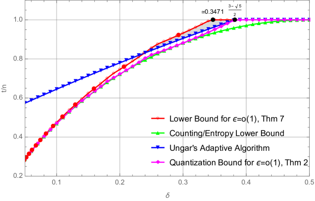
Figure 1: Bounds on $t/n$ vs. $\delta$ for $\epsilon=o(1)$. The lower bound implied by theorem 1 corresponds to the horizontal part of the magenta curve, and the result implied by theorem 2 corresponds to the remainder of the magenta curve (the “Quantization bound”). Both of these are superseded by the more sophisticated (and harder to prove) lower bound in theorem 7, plotted via the red curve. The shaded region (above the blue curve and below the red curve) denotes where there is an “adaptivity gap” – the lower bound for (vanishing-error) NAGT exceeds the rate achievable by (zero-error) AGT [25].

Estimation/inverse problems are the bread and butter of engineering – given a system with a known input-output relationship, an observed output, and statistics on the input, the goal is to infer the input. While much is known about linear estimation problems and their fundamental limits [16, 22], understandably characterizing the fundamental limits of non-linear estimation problems are considerably more challenging.

Arguably one of the “simplest” non-linear estimation problems is that of Group Testing (GT). It is assumed that hidden among a set of $n$ items is a special set ${{\mathcal{D}}}$ of $d$ defective items. The classical problem as posed by Dorfman [8], requires one to exactly estimate ${{\mathcal{D}}}$ via disjunctive measurements (“group tests”) on “pools” of items. That is, the output of each test is positive if the pool contains at least one item from ${{\mathcal{D}}}$, and negative otherwise. Besides its intrinsic appeal as a fundamental estimation problem, group-testing and its generalizations have a variety of diverse applications, such as bioinformatics [21], wireless communications [28, 3], and pattern finding [17].

Group testing problems come in a variety of flavours. In particular:

1. (Non)-Adaptivity: The testing algorithm can be adaptive (tests may be designed depending on previous test outcomes) or non-adaptive (tests must be designed non-adaptively, allowing for parallel testing/standardized hardware).

2. Reconstruction error: The reconstruction algorithm might need to be zero-error (always output the correct answer), or vanishing error (the probability of error goes to zero asymptotically in $n$), or an $\epsilon$ probability of error ($\epsilon$-error) may be allowed.

3. Statistics of ${\mathcal{D}}$: Different works consider different statistical models for ${\mathcal{D}}$. In Combinatorial Group Testing (CGT), it is assumed that any set of $d$ items may be defective, whereas in Probabilistic Group Testing (PGT), items are assumed to be i.i.d. defective with probability $d/n$.

4. Sparsity regime: Finally, it turns out that the specific sparsity regime matters - the regime where $d$ scales sub linearly in $n$ has seen much work, whereas the linear sparsity regime ($d=\delta n$ for some constant $\delta$) is relatively little explored.

In this work we focus on non-adaptive group-testing with $\epsilon$-error in the linear sparsity regime – indeed, this is perhaps the most “natural” version of the problem, especially when viewed through an information-theoretic lens (for instance, the most investigated/used versions of channel codes are: non-adaptive since the encoder does not get to see the decoder’s input; allow for reconstruction error; and typically have constant rate and hence are in the linear regime). Nonetheless, to put our own results in context we first briefly reprise the literature for other flavors of the problem in table 1. Note that, with a slight abuse of notation, we denote by $H(X)$ the entropy of the random variable/vector $X$, as well as the binary entropy function $H(x)=-x\log x-(1-x)\log(1-x)$. This should be clear from the argument of the function.

In particular, let us briefly discuss the existing results of $\epsilon$-error nonadaptive group testing problem, the focus of this paper. It is quite straightforward to come up with a converse result based on counting/Fano’s inequality (for example, see [4]) that says $t\geq(1-\epsilon)\log\binom{n}{d}$. In [1], it has been shown that this bound is also tight for small $\epsilon$, as long as $d=O(n^{1/3})$ by showing randomized achievability schemes. Probabilistic existence of achievability schemes in this regime has also been derived, including for more general settings, in [31] (see Theorem 5.5 therein). If we are allowed to sacrifice a constant factor in the number of tests, then we can have explicit deterministic construction of such achievability schemes [19]. It is to be noted that, there is a surprising lack of study in the regime where the number of defectives varies linearly with the number of elements, i.e., $d=\delta n$. The counting converse bound simply boils down to $t\geq nH(\delta).$ This implies that individual testing of items is optimal when $\delta>0.5$. There is no other nontrivial converse bound that exists for the linear regime. In this paper we aim to close this gap. On the other hand, a recent work by Wadayama [26], provides an achievability scheme in this regime based on sparse-graph codes (and density-evolution analysis). For certain values of $\delta$ (for example $\delta=1-\frac{1}{2^{1/6}}$), this achievability scheme is in direct contradiction with our impossibility result in theorem 7.

It also is worth pointing out that the linear-sparsity regime is well-studied for adaptive group testing starting as early as in the sixties. It has been shown that under a zero probability of error metric, for $\delta>\frac{3-\sqrt{5}}{2}$ individual testing is the optimal strategy [25].  On the other hand, a rather simple adaptive algorithm achieves an expected number of tests equaling at most $0.5(3-(1-\delta)-(1-\delta)^{2})n$ and identifies all defectives [25] – we reprise this algorithm for completeness in section A.2. This is interesting if we contrast this with our converse result. There is a regime of values of $\delta$ (roughly in the range $\delta\in(0.3471,0.3819)$), where zero-error adaptive algorithms on average require fewer than $n$ tests to reconstruct ${\mathcal{D}}$, however our bounds imply that the best nonadaptive algorithm (even with vanishing error) turns out to essentially be individual testing of each element.

[c] Adaptive Non-Adaptive Zero-error^∗1 Zero-error Vanishing Error / $\epsilon$-error sub-linear linear $d=\delta n$ sub-linear $d=n^{\beta}$ linear $d=\delta n$ sub-linear $d=n^{\beta}$ linear $d=\delta n$ Achievability $d\log(n/d)+O(d)$ [14] $0.5(3-(1-\delta)-(1-\delta)^{2})n$ [25] $d^{2}\log n$ [15] $n$ $c(\beta)(1+\epsilon)(1-\beta)d\log(n)$, [1]^∗4 See discussion of [26] Converse $d\log(n/d)$ (folklore) $nH(\delta)$ [4]^∗2, $n-1$ if $\delta>\log_{3}(1.5)\approx 0.3691$, (Max. # tests) [23] ^∗3, $n$ if $\delta>\frac{3-\sqrt{5}}{2}\approx 0.3819$, (Avg. # tests)[25] ^∗3 $\frac{d^{2}}{2\log d}\log n$ [10] $n$ if $\beta\geq 1/2$ [9, Thm 7.2.9] $n$ [9, Thm 7.2.9] $(1-\epsilon)(1-\beta)d\log(n)$ [4] $n(1-\epsilon)$ $\delta\gtrsim 0.3471$ $g_{\delta}^{-1}(H(\delta)-\epsilon)$ $\delta\lesssim 0.3471$ (see theorem 7) • *1 Adaptive algorithms with reconstruction error have not really been considered much in the literature. Most proposed algorithms naturally result in zero-error, and the only known converses that are tighter than the counting bound intrinsically rely on the zero-error nature of the problem. • *2 This bound holds even for $\epsilon$-error. • *3 It is known [25] that $\frac{3-\sqrt{5}}{2}\approx 0.382$ is the correct cutoff point for adaptive PGT, whereas it is conjectured that the cutoff point for adaptive CGT is 1/3 [13] • *4 $c(\beta)\triangleq\begin{cases}=1&\beta<1/3\\ >1&\beta\in(1/3,1)\end{cases}$

Table 1: A comparison of known inner and outer bounds on the number of tests required in a variety of group-testing settings. See also fig. 1.

1.1 Our Contributions and Techniques

The canonical method (variously called the information-theoretic bound, or the counting bound) for proving impossibility results for group-testing problems via information-theoretic methods is quite robust to model perturbations: it works for adaptive and non-adaptive algorithms, zero-error and vanishing error reconstruction error criteria, PGT and CGT, and sub-linear and linear regimes. This method (see the Appendix in [4] for an example) generally proceeds as follows:

1. Entropy bound on input: One first bounds the entropy $H({\boldsymbol{X}}_{[n]})$ of the $n$-length binary vector ${\boldsymbol{X}}_{[n]}$ describing the status of the $n$ items (this means, the entry corresponding to an element in ${\boldsymbol{X}}_{[n]}$ is $1$ if and only if the element is defective): this quantity equals $\log\lparen\binom{n}{d}\rparen$ in the CGT case, and $nH(d/n)$ in the PGT case; then

2. Information (in)equalities/Fano’s inequality: One uses standard information equalities, the data-processing inequality, the chain-rule, and Fano’s inequality to argue that any group-testing scheme must satisfy the inequality $H({\boldsymbol{Y}}_{[t]})\geq H({\boldsymbol{X}}_{[n]})-n\epsilon$ (here ${\boldsymbol{Y}}_{[t]}$ is a binary vector describing the set of $t$ test outcomes (that means an entry in ${\boldsymbol{Y}}_{[t]}$ is $1$ if and only if the corresponding test result is positive), and $\epsilon$ is a lower bound on the probability of error of the group-testing scheme); and then

3. Independence bound. Since ${\boldsymbol{Y}}_{[t]}$ is a binary vector, one uses the independence bound to argue that $H({\boldsymbol{Y}}_{[t]})\leq t$, and thereby obtains a lower bound on the required number of tests $t$, as a function of $\epsilon$, and $H({\boldsymbol{X}}_{[n]})$.

Perhaps surprisingly, even for such a non-linear problem as group-testing, for a variety of group-testing flavors (such as non-adaptive GT with vanishing error when $d={\mathcal{O}}(n^{1/3})$ [1]) such a straightforward approach results in an essentially tight lower bound on the number of tests required. The key contribution of our work is to provide a tightening of the method above for the regimes where it is not known to be tight.

While we believe our generalization technique is also fairly robust to various perturbations of the group-testing model, we focus in this work on the problem of $\epsilon$-error non-adaptive PGT in the linear sparsity regime. Possibly our key insight is that for this problem variant is that step (iii) of the counting bound may be quite loose.

Specifically, we present three novel converse bounds in theorems 1, 2 and 7 for the general non-adaptive PGT problem in the linear regime. The result in theorem 1 follows from the observation that, for $\delta\geq\frac{3-\sqrt{5}}{2}$ the individual test entropies are maximized when each test contains exactly one object. Another simple result, for $\delta\leq\frac{3-\sqrt{5}}{2}$, in theorem 2 follows from the observation that the individual test entropy, satisfies $H(Y_{l})\lneq 1$ for most of the region $\delta\in(0,1)$ because of the constraint that each test must contain an integer number of objects.

Our main result (tighter than either theorem 1 or theorem 2, but also significantly more challenging to prove) in theorem 7 exploits the observation that the tests in the Non Adaptive Group Testing (NAGT) problem must have elements in common. For the linear regime, this observation leads to significant mutual information between the tests when the number of objects in the tests do not scale with $n$. Hence, we can exploit this mutual information to tighten the upper bound on the joint entropy $H({\boldsymbol{Y}}_{[t]})$ in step (iii) above. Figure 1 plots our results in the linear regime along with existing results in the literature.

To bound the joint entropy $H({\boldsymbol{Y}}_{[t]})$ in step (iii), we must look for information inequalities that upper bound the joint entropies of correlated random variables. While the fascinating polymatroidal properties of such joint entropies (Shannon-type inequalities) explored by Zhang and Yeung [30], as well as the non-Shannon-type inequalities that were subsequently found [29] and are not consequences of such polymatroidal properties, are in this direction, they are perhaps too general to offer much guidance as to which specific information-inequalities might prove useful for providing non-trivial lower bounds for NAGT. A more structured characterization in this direction is Han’s inequality [12] (implied by Shannon-type inequalities), that says

$$H({\boldsymbol{Y}}_{[t]})\leq\frac{1}{t-1}\sum_{i=1}^{t}H({\boldsymbol{Y}}_{[t]\setminus\{i\}}),$$

where ${\boldsymbol{Y}}_{[t]\setminus\{i\}}$ contains test results except for the $i$th test.

In this paper we use a significant generalization of Han’s inequality to an asymmetric setting due to Madiman and Tetali [18], that seems well-suited to analyzing the combinatorial structures naturally arising in NAGT. Consider the NAGT matrix $M\in\{0,1\}^{t\times n}$, whose $(i,j)$th element is 1 if and only if the $i$th test includes the $j$th element. Let ${\boldsymbol{Y}}_{S}$ denote the binary random variables corresponding to the test outcomes for $S\subseteq[t]$ and let ${\boldsymbol{X}}_{S}$ denote the indicator random variables corresponding to the objects for $S\subseteq[n]$. To demonstrate that non-trivial correlation between at least some sets of tests that must exist in our setting, we use the Madiman-Tetali inequalities [18],

$$H({\boldsymbol{Y}}_{[t]})\leq\sum_{S\in{\mathcal{C}}}\alpha(S)H({\boldsymbol{Y}}_{S}|{\boldsymbol{Y}}_{S_{-}})$$ (1)

where $S_{-}\triangleq\{i\in[t]:i\lneq j,\forall j\in S\}$ and ${\mathcal{C}}\subseteq 2^{[t]}$. The coefficients $\alpha(S)$ and the set ${\mathcal{C}}$ form a cover of $2^{[t]}$ (more detail on this will be given in section 2). In theorem 7 we use the weak form eq. 24 of the inequality above – see section 4 for a discussion of the strong form and its potential use.

We use a two-step procedure to bound the joint entropy. In the first step, we assume that all the rows of the matrix $M$ has same weight (i.e., all tests contain the same number of elements, section 2.5). The results are then extended to general group testing matrices by considering them as a union of tests of (differing) constant weights. The final result is summarized in theorem 7.

In the rest of the paper, we first describe our converse results section 2, followed by a comparison with earlier bounds section 3 and future directions of this project.

2 Impossibility Results for Nonadaptive Group Testing

2.1 Notation and Model

For integers $a,b$ let $[a,b]\triangleq\{a,a+1,\ldots,b\}$ and $[b]\triangleq[1,b]$. Let $\log(.)$ denote the logarithm to the base 2, unless otherwise stated.

Consider the PGT problem with $n$ objects. Assume that we can tolerate a error probability $\epsilon$ in the decoding. Denote the indicator random variable which corresponds to object $i\in[n]$ being defective by $X_{i}$. Then $X_{i}$ are iid $\operatorname{Bernoulli}(\delta)$. With a slight abuse of notation, we use $X_{i}$ to refer to the random variable and the object $i$ interchangeably, when there is no scope of confusion.

Let $M\in\{0,1\}^{t\times n}$ denote the fixed GT matrix with $t$ tests. Denote the random variable corresponding to the outcome of the test in row $l$ by $Y_{l}$ and let ${\boldsymbol{Y}}_{S}\triangleq\{Y_{l}\}_{l\in S}$ for $S\subset[t]$. For an object set $R\subseteq[n]$, let $Y(R)$ denote the random variable corresponding to the test with object set $R$. For a class of object sets ${\mathcal{R}}\subseteq 2^{[n]}$, let ${\boldsymbol{Y}}({\mathcal{R}})$ denote the random vector corresponding to the test with object sets $R\in{\mathcal{R}}$.

Let $R_{l}\subseteq[n],l\in[t]$ denote the set of objects included in test $Y_{l}$ and let $S_{i}\subseteq[t],i\in[n]$ denote the tests containing the object $i$. Let ${\mathcal{R}}(S),S\subseteq[t]$ denote the class of subsets of $[n]$ corresponding to the object sets of the tests $\{Y_{l}\}_{l\in S}$ ie. ${\mathcal{R}}\lparen S\rparen\triangleq\{R_{l}\}_{l\in S}$. For a class of sets ${\mathcal{X}}\subseteq 2^{\Omega}$, and $A\in 2^{\Omega}$ define ${\mathcal{X}}-A\triangleq\{Q\setminus A:Q\in{\mathcal{X}}\}$ as the class with set $A$ removed from all subsets in ${\mathcal{X}}$ and let $\displaystyle[{\mathcal{X}}]\triangleq\bigcup_{A\in{\mathcal{X}}}A$.

2.2 Simple Converse Bounds

Recall that in the linear sparsity regime each element is defective with probability $d/n=\delta$. The canonical counting bound for the Group Testing problem gives the following upper bound on the number of tests for the $\epsilon$-error case:

$$t/n\geq H(\delta)-\epsilon$$ (2)

This method uses the independence bound to get an upper bound on the joint entropy of the tests, eq. 3, and then uses Fano’s inequality, eq. 4, to get a a lower bound on $t$.

$$H({\boldsymbol{Y}}_{[t]})\leq t$$ (3)

$$\underbrace{H({\boldsymbol{X}}_{[n]})}_{=nH(\delta)}\leq H(Y_{[t]})+\epsilon n.$$ (4)

We tighten eq. 2 by improving the bound in eq. 3 for the non-adaptive PGT problem in the linear regime. We do this by exploiting the fact the in the NAGT problem there would be a significant fraction of tests that have elements in common. Intuitively, we would want to maximize the entropy of the individual tests $\{Y_{l}\}_{l\in{[t]}}$ by choosing $\lvert R_{l}\rvert$ such that $H(Y_{l})=H((1-\delta)^{\lvert R_{l}\rvert})=1$ i.e. $R_{l}\approx k_{0}(\delta)$ for $l\in{[t]}$ where

$$k_{0}(\delta)\triangleq\frac{\log\lparen 1/2\rparen}{\log(1-\delta)}$$ (5)

This implies that all tests contain a constant (with respect to $n$) number of objects. When any set $S\subseteq[t]$ of such tests ${\boldsymbol{Y}}_{S}$ have an object in common, we can bound their joint entropy away from $\lvert S\rvert$. We exploit this fact to bound the joint entropy $H({\boldsymbol{Y}}_{[t]})$ away from $t$. But first, we exploit the nature of the group tests to improve eq. 2.

Theorem 1.

For the PGT problem, we need at least $n(1-\epsilon/H(\delta))$ tests to identify the defective set with error probability $\epsilon$ for $\delta\geq\delta^{\star}$ where

$$\delta^{\star}\triangleq\frac{3-\sqrt{5}}{2}$$

.

Proof.

Using the entropy chain rule, for $\delta\geq\delta^{\star}$, we have,

$$H({\boldsymbol{Y}}_{[t]}) \leq\sum_{l\in[t]}H(Y_{l})$$ (6a)

$$=\sum_{l\in[t]}H((1-\delta)^{\lvert R_{l}\rvert})$$ (6b)

$$\leq tH(1-\delta)=tH(\delta)$$ (6c)

Inequality 6c is obvious for $\delta\geq 1/2$. For $\delta\in[\delta^{\star},1/2)$, $(1-\delta)^{2}\leq\delta<1/2\implies H((1-\delta)^{2})\leq H(\delta)=H(1-\delta)$. Hence, eq. 6c follows here as well. Now, using eq. 4 and eq. 6c we get,

$$t\geq n(1-\epsilon/H(\delta))$$

∎

Thus, for $\delta\geq\delta^{\star}$ we cannot do any better than individual testing. In the rest of the section, we focus on the GT bound for $\delta\leq\delta^{\star}$. Even in this regime, we can use the fact that eq. 5 is not an integer for all values of $\delta$ to improve eq. 2 without much effort.

Theorem 2.

[Quantization Bound]

$$t/n\geq\frac{H(\delta)-\epsilon}{\displaystyle\max_{k\in{\mathbb{N}}}H((1-\delta)^{k})}$$

Proof.

Due to the fact that each test can contain only an integer number of objects, we have

$$H(Y_{l})=H((1-\delta)^{\lvert R_{l}\rvert})\leq\max_{k\in{\mathbb{N}}}H((1-\delta)^{k})$$

$$\implies H({\boldsymbol{Y}}_{[t]})\leq\sum_{l\in[t]}H(Y_{l})\leq t\max_{k\in{\mathbb{N}}}H((1-\delta)^{k})$$ (7)

Hence theorem 2 follows from eq. 4 and section 2.2. ∎

Note that, for $\delta\notin\{1-\frac{1}{2^{1/k}}\}_{k\in{\mathbb{N}}}$, $\max_{k\in{\mathbb{N}}}H((1-\delta)^{k})\lneq 1$. Therefore, the result in theorem 2 improves over the classical counting bound.

2.3 Upper Bound via Madiman Tetali inequality

To improve eq. 3 further for all values of $\delta\leq\delta^{\star}$, we use the Madiman Tetali inequalities in [18] to exploit the correlation between tests,

$$H({\boldsymbol{Y}}_{[t]})\leq\sum_{S\in{\mathcal{C}}}\alpha(S)H({\boldsymbol{Y}}_{S})$$ (8)

where ${\mathcal{C}}$ are a class of subsets of $[t]$ that cover $[t]$, and $\{\alpha(S)\}_{S\in{\mathcal{C}}}$ denote a fractional cover of the hypergraph ${\mathcal{C}}$ on vertex set $[t]$. This means that for each $i\in[t]$, the set of numbers $\{\alpha(S)\}_{S\in{\mathcal{C}}}$ satisfy the relation $\sum_{S\in{\mathcal{C}}:i\in S}\alpha(S)\geq 1$.

Note that using the independence bound for $H({\boldsymbol{Y}}_{S})$ in eq. 8 we have,

$$H({\boldsymbol{Y}}_{[t]})\leq\sum_{S\in{\mathcal{C}}}\alpha(S)\lvert S\rvert$$ (9)

where $\sum_{S\in{\mathcal{C}}}\alpha(S)\lvert S\rvert\geq t$. Therefore, to improve eq. 3 we have to utilize the fact that ${\boldsymbol{Y}}_{S}$ have joint entropy less than $\lvert S\rvert$. Heeding this intuition, first for a fixed set $S\subseteq[t]$, we derive a non-trivial upper bound on $H({\boldsymbol{Y}}_{S})$ in section 2.4, for tests ${\boldsymbol{Y}}_{S}$ such that all of them have at least one object $X\in\{X_{i}\}_{i\in[n]}$ in common ie $X\in\cap_{l\in S}R_{l}$. Next, we use this bound to derive a closed-form expression for the joint entropy $H({\boldsymbol{Y}}_{[t]})$ in eq. 8 for a constant row weight NAGT matrix $M$ in section 2.5. Finally, we generalize the upper bound to derive a closed form expression for arbitrary row weight matrices in section 2.6. Using this expression and eq. 4, we get an improvement over the counting lower bound in theorem 7.

2.4 Upper bound on $H({\boldsymbol{Y}}_{S})$

Consider a set $S\subseteq[t]$ such that there exists an object $X\in\{X_{i}\}_{i\in[n]}$ that is common in all the tests ${\boldsymbol{Y}}_{S}$. Also assume that, $\lvert R_{l}\rvert=k,\forall l\in S$. In this case, we upper bound the joint entropy of the tests ${\boldsymbol{Y}}_{S}$ in theorem 3.

Theorem 3.

Consider $S\subseteq[t]$, such that $\lvert R_{l}\rvert=k$, $\forall l\in S$ and all tests ${\boldsymbol{Y}}_{S}$ have at least one object in common. Then,

$$H({\boldsymbol{Y}}_{S})\leq(1-\delta)\lvert S\rvert H((1-\delta)^{k-1})+H(\delta)-f_{\delta,k}(\lvert S\rvert)$$ (10)

where

$$f_{\delta,k}(s)\triangleq(\delta+(1-\delta){p_{\delta,k}}^{s})H\left(\frac{\delta}{\delta+(1-\delta){p_{\delta,k}}^{s}}\right)$$ (11)

and

$$p_{\delta,k}\triangleq(1-(1-\delta)^{k-1})$$ (12)

In the rest of this section, we give the proof of theorem 3. Assume that the tests ${\boldsymbol{Y}}_{S}$ have object $X\in\{X_{i}\}_{i\in[n]}$ in common. Let ${\boldsymbol{Y}}^{\prime}_{S}$ denote the set of tests containing the same objects as ${\boldsymbol{Y}}_{S}$ but with object $X$ removed from all tests ie. ${\boldsymbol{Y}}^{\prime}_{S}\triangleq{\boldsymbol{Y}}({\mathcal{R}}(S)-\{X\})$. We have,

$$H({\boldsymbol{Y}}_{S})=H({\boldsymbol{Y}}_{S}|X)+H(X)-H(X|{\boldsymbol{Y}}_{S})$$ (13)

$$H({\boldsymbol{Y}}_{S}|X)=(1-\delta)H({\boldsymbol{Y}}^{\prime}_{S})\leq\lvert S\rvert(1-\delta)H((1-\delta)^{k-1})$$ (14)

$$H(X)=H(\delta)$$ (15)

$$H(X|{\boldsymbol{Y}}_{S})=(\delta+(1-\delta)\operatorname{Pr}\left\lparen{\boldsymbol{Y}}^{\prime}_{S}={\bf{1}}\right\rparen)H\left(\frac{\delta}{\delta+(1-\delta)\operatorname{Pr}\left\lparen{\boldsymbol{Y}}^{\prime}_{S}={\bf{1}}\right\rparen}\right)$$ (16)

Therefore, combining eq. 13, eq. 14, eq. 15, and eq. 16, we have

$$H({\boldsymbol{Y}}_{S}) \leq(1-\delta)H((1-\delta)^{k-1})+H(\delta)-H(X|{\boldsymbol{Y}}_{S})$$ (17)

Note that,

$$\frac{\partial(\delta+(1-\delta)x)H(\frac{\delta}{\delta+(1-\delta)x})}{\partial x}=(1-\delta)\log\left\lparen 1+\frac{\delta}{x(1-\delta)}\right\rparen\geq 0$$ (18)

Thus, the expression for $H(X|{\boldsymbol{Y}}_{S})$ in eq. 16 is minimized at the minimum possible value of $\operatorname{Pr}\left\lparen{\boldsymbol{Y}}^{\prime}_{S}={\bf{1}}\right\rparen$. We lower bound the probability $\operatorname{Pr}\left\lparen{\boldsymbol{Y}}^{\prime}_{S}=\bf{1}\right\rparen$ using lemma 4 to get an upper bound on eq. 17.

Lemma 4.

For any $S\subseteq[t]$, we have,

$$\min_{\begin{subarray}{c}R_{l}\in{\mathcal{R}}(S):\\ \lvert R_{l}\rvert=r_{l}\end{subarray}}\operatorname{Pr}\left\lparen{\boldsymbol{Y}}_{S}={\bf 1}\right\rparen=\prod_{l\in S}(1-(1-\delta)^{r_{l}})$$ (19)

Proof.

Note that $\operatorname{Pr}\left\lparen Y_{l}=1\right\rparen=(1-\delta)^{\lvert R_{l}\rvert}$. We show that the minimization in eq. 22 occurs when all object sets $\{R_{l}\}_{l\in S}$ are disjoint. Since, in that case the tests in ${\boldsymbol{Y}}_{S}$ are independent, we must have,

$$\min_{\begin{subarray}{c}R_{l}\in{\mathcal{R}}(S):\\ \lvert R_{l}\rvert=r_{l}\end{subarray}}\operatorname{Pr}\left\lparen{\boldsymbol{Y}}_{S}={\bf 1}\right\rparen =\prod_{l\in S}\operatorname{Pr}\left\lparen Y_{l}={1}\right\rparen$$ (20)

$$=\prod_{l\in S}(1-(1-\delta)^{r_{l}})$$

Without loss of generality, let $S=[s]$. Suppose that, the tests ${\boldsymbol{Y}}_{S}$ are such that there exists an object $i$ that is common among tests $Y_{1},Y_{2},\ldots,Y_{a}$ for some $a\in[2,\lvert S\rvert]$. Then, we show that, we can decrease the probability $\operatorname{Pr}\left\lparen{\boldsymbol{Y}}_{S}=\bf{1}\right\rparen$ by modifying $R_{1}$ to $R_{1}^{\ast}$ by including an object ${i^{\ast}}\in[n]\setminus[{\mathcal{R}}(S)]$ in $Y_{1}$ instead of object $i$ such that $R_{1}^{\ast}=(R_{1}\setminus\{i\})\cup\{i^{\ast}\}$. Denote the modified tests by ${\boldsymbol{Y}}_{S}^{\ast}$. Then, it suffices to prove that,

$$\operatorname{Pr}\left\lparen{\boldsymbol{Y}}_{S}=\bf{1}\right\rparen\geq\operatorname{Pr}\left\lparen{\boldsymbol{Y}}^{\ast}_{S}=\bf{1}\right\rparen$$ (21)

since using eq. 21 recursively for objects contained in more than one tests in ${\boldsymbol{Y}}_{S}^{\ast}$ we can prove eq. 20. We prove eq. 21 in section A.1. ∎

Thus, from lemma 4 we have,

$$\operatorname{Pr}\left\lparen{\boldsymbol{Y}}^{\prime}_{S}=\bf{1}\right\rparen\geq p_{\delta,k}^{\lvert S\rvert},\;\forall i\in[n]$$ (22)

where $p_{\delta,k}$ is defined in eq. 12. Hence, from eq. 16, eq. 18, and eq. 22, we have,

$$H(X|{\boldsymbol{Y}}_{S})\geq f_{\delta,k}(\lvert S\rvert)$$ (23)

Now, combining eqs. 17 and 23 we have,

$$H({\boldsymbol{Y}}_{S})\leq(1-\delta)\lvert S\rvert H((1-\delta)^{k-1})+H(\delta)-f_{\delta,k}(\lvert S\rvert)$$

where $f_{\delta,k}(s)$ is as defined in eq. 11.

2.5 Constant Row Weight Testing Matrix

In this section we assume that matrix $M$ has constant row weight $k$ such that $k\geq 2$. Intuitively, this is a very natural assumption. Since it allows each test in matrix $M$ to be symmetric. This assumption also allows us to easily upper bound the joint entropy of the tests $H({\boldsymbol{Y}}_{[t]})$ using eq. 8, as we see below.

To apply eq. 8, we consider the hypergraph ${\mathcal{C}}$ with $n$ edges and having matrix $M$ as the incidence matrix. Thus, ${\mathcal{C}}\triangleq\{S_{i}\}_{i=1}^{n}$, where $S_{i}$ denotes the support set of column $i$ in $M$. Note that, in this case, $\alpha(S_{i})=\frac{1}{k}$ forms a cover of the hypergraph ${\mathcal{C}}$. Therefore, we have,

$$H({\boldsymbol{Y}}_{[t]})\leq\frac{1}{k}\sum_{i=1}^{n}H({\boldsymbol{Y}}_{S_{i}})$$ (24)

We upper bound the expression on the RHS in eq. 24 to get an asymptotic closed form expression for the joint entropy of the form,

$$\frac{H({\boldsymbol{Y}}_{[t]})}{n}\leq g_{\delta,k}(t/n)$$ (25)

where $g_{\delta,k}(T)$ is shown to be an increasing function of $T$. Thus, using eq. 4, we have,

Theorem 5.

Consider the non-adaptive PGT problem, with tolerable probability of error $\epsilon$. Assume that each object is defective independently with probability $\delta$. Then, for a constant row weight $k$ group testing matrix, we have asymptotically in $n$,

$$\frac{t}{n}\geq g_{\delta,k}^{-1}(H(\delta)-\epsilon)$$ (26)

where $g_{\delta,k}^{-1}(x)\triangleq y$ such that $g_{\delta,k}(y)=x$ and

$$g_{\delta,k}(T)\triangleq T(1-\delta)H((1-\delta)^{k-1})+\frac{1}{k}\left\lparen H(\delta)-f_{\delta,k}(k\;T)\right\rparen$$ (27)

where $f_{\delta,k}(T)$ is defined in eq. 11.

The proof of theorem 5 follows from eq. 25 and eq. 4. The form of $g_{\delta,k}(T)$ in eq. 25 is derived below as

$$H({\boldsymbol{Y}}_{[t]}) \leq t(1-\delta)H((1-\delta)^{k-1})+\frac{n}{k}H(\delta)-\frac{1}{k}\sum_{i=1}^{n}f_{\delta,k}(\lvert S\rvert)$$ (28)

$$\leq t(1-\delta)H((1-\delta)^{k-1})+\frac{n}{k}\left\lparen H(\delta)-f_{\delta,k}\left(\frac{1}{n}\sum_{i=1}^{n}\lvert S\rvert\right)\right\rparen$$ (29)

$$=t(1-\delta)H((1-\delta)^{k-1})+\frac{n}{k}\left\lparen H(\delta)-f_{\delta,k}(kt/n)\right\rparen$$ (30)

$$=ng_{\delta,k}(t/n)$$

where eq. 28 follows from theorem 3 and eq. 24, and eq. 29 follows from the convexity of $f_{\delta,k}(s)$ from lemma 6. Note that since $f_{\delta,k}(s)$ is a convex decreasing function of $s$, $g_{\delta,k}(T)$ must be a concave increasing function of $T$. Thus, eq. 25 and hence theorem 5 follows.

Lemma 6.

$f_{\delta,k}(s)\triangleq(\delta+(1-\delta){p_{\delta,k}}^{s})H(\frac{\delta}{\delta+(1-\delta){p_{\delta,k}}^{s}})$ is a convex decreasing function of $s$

Proof.

We have,

$$\frac{\partial f_{\delta,k}(s)}{\partial s}=(1-\delta)p_{\delta,k}^{s}\ln p_{\delta,k}\log\left\lparen 1+\frac{c}{(1-c)p_{\delta,k}^{s}}\right\rparen<0$$ (31)

and

$$\frac{\partial^{2}f_{\delta,k}(s)}{\partial s^{2}}=\frac{(\ln p_{\delta,k})^{2}}{\ln 2}y\left\lparen\underbrace{\ln(1+\delta/y)-\frac{\delta/y}{1+\delta/y}}_{\Psi(\delta/y)}\right\rparen>0$$ (32)

where $y=(1-\delta)p_{\delta,k}^{s}$. Since $\Psi(z)\triangleq\ln(1+z)-\frac{z}{1+z}$ is always positive for $z>0$, $f_{\delta,k}(s)$ is a decreasing convex function of $s$ from eqs. 32 and 31. ∎

2.6 General Testing Matrix

In this section, we remove the assumption that matrix $M$ has a fixed row weight $k$ and derive an upper bound on $H({\boldsymbol{Y}}_{[t]})$ – better than eq. 3 – for the most general case. We use this upper bound to improve eq. 2 in theorem 7.

We separate the matrix $M$ into submatrices $\{M_{k}\}_{k}\in\{0,1\}^{t_{k}\times n}$ based on the number of objects in the tests. Thus, matrix $M_{k}$ has $t_{k}=\alpha_{k}t$ tests of weight $k$ such that $\sum_{k=1}^{\infty}\alpha_{k}=1$.

Now, we show that the analysis in section 2.5 follows through for each matrix $M_{k}$. Let $t_{0}\triangleq 0$. Assume w.l.o.g. that the tests corresponding to $M_{k}$ are ${\boldsymbol{Y}}_{[t_{k-1}+1,t_{k}]}$. Denote the support sets of column $i$ in $M_{k}$ by $S_{k,i}$. Note that some of the columns in the matrix may be empty, i.e. $\lvert S_{k,i}\rvert=0$. Thus let ${\mathcal{C}}_{k}^{\prime}$ denote the support sets corresponding to the non-empty columns. Let ${\mathcal{C}}_{k}$ denote the class of support sets $\{S_{k,i}\}_{i\in[n]}$ where each empty column is considered a distinct set. Therefore we have,

$$H({\boldsymbol{Y}}_{[t_{k-1}+1,t_{k}]}) \leq\sum_{S_{k,i}\in{\mathcal{C}}_{k}^{\prime}}\alpha(S)H({\boldsymbol{Y}}_{S})$$

$$=\frac{1}{k}\sum_{S_{k,i}\in{\mathcal{C}}_{k}^{\prime}}H({\boldsymbol{Y}}_{S_{k,i}}|X_{i})+H(X_{i})-H(X_{i}|{\boldsymbol{Y}}_{S_{k,i}})$$ (33)

When $\lvert S_{k,i}\rvert=0$, we have $H(X_{i}|{\boldsymbol{Y}}_{S_{k,i}})=H(X_{i})$ and $H({\boldsymbol{Y}}_{S_{k,i}}|X_{i})=0$. Note that for $\lvert S_{k,i}\rvert=0$ the lower bound in eq. 23 also gives $H(X_{i}|{\boldsymbol{Y}}_{S_{k,i}})\leq f_{\delta,k}(0)=H(\delta)$. Therefore,

$$\sum_{S_{k,i}\in{\mathcal{C}}_{k}\setminus{\mathcal{C}}_{k}^{\prime}}\left\lparen H({\boldsymbol{Y}}_{S_{k,i}}|X_{i})+H(X_{i})-H(X_{i}|{\boldsymbol{Y}}_{S_{k,i}})\right\rparen=0$$ (34)

Hence, combining sections 2.6 and 34 we have

$$H({\boldsymbol{Y}}_{[t_{k-1}+1,t_{k}]}) \leq\frac{1}{k}\sum_{S_{k,i}\in{\mathcal{C}}_{k}}\left\lparen H({\boldsymbol{Y}}_{S_{k,i}}|X_{i})+H(X_{i})-H(X_{i}|{\boldsymbol{Y}}_{S_{k,i}})\right\rparen$$ (35)

Remark.

Note that the manipulation in eq. 34, although seemingly unnecessary, is required because $\lvert S_{i}\rvert=0$ is not possible in section 2.5. But since this is possible in this section with non-constant weight GT matrices, the lower bound of $H(X_{i}|{\boldsymbol{Y}}_{S_{k,i}})$ in eq. 23 may not hold in this case. But this algebraic manipulation resolves that problem.

Using the expressions in eq. 14, eq. 15 and eq. 23 in eq. 35, we have,

$$H({\boldsymbol{Y}}_{[t_{k-1}+1,t_{k}]}) \leq\frac{1}{k}\sum_{S_{k,i}\in{\mathcal{C}}_{k}}\left\lparen H({\boldsymbol{Y}}_{S_{k,i}}|X_{i})+H(X_{i})-H(X_{i}|{\boldsymbol{Y}}_{S_{k,i}})\right\rparen$$

$$\leq t_{k}(1-\delta)H((1-\delta)^{k-1})+\frac{n}{k}\left\lparen H(\delta)-f_{\delta,k}\left(\frac{1}{n}\sum_{i\in[n]}\lvert S_{k,i}\rvert\right)\right\rparen$$

$$\iff\frac{H({\boldsymbol{Y}}_{[t_{k-1}+1,t_{k}]})}{n} \leq(t_{k}/n)(1-\delta)H((1-\delta)^{k-1})+\frac{1}{k}\left\lparen H(\delta)-f_{\delta,k}\left(\frac{k\;t_{k}}{n}\right)\right\rparen$$

$$=\alpha_{k}\frac{t}{n}(1-\delta)H((1-\delta)^{k-1})+\frac{1}{k}\left\lparen H(\delta)-f_{\delta,k}\left(k\alpha_{k}\frac{t}{n}\right)\right\rparen$$

$$=g_{\delta,k}\left(\frac{\alpha_{k}t}{n}\right)$$ (36)

where for $k=1$, we define,

$$g_{\delta,1}(T)\triangleq TH(\delta).$$ (37)

Thus, we have from section 2.6,

$$\frac{H({\boldsymbol{Y}}_{[t]})}{n} \leq\sum_{k\geq 1}\frac{H({\boldsymbol{Y}}_{[t_{k-1}+1,t_{k}]})}{n}$$ (38)

$$\leq\sum_{k\geq 1}g_{\delta,k}(\alpha_{k}t/n)$$ (39)

$$\leq\max_{\begin{subarray}{c}\{\alpha_{k}\}_{k}\\ :\sum_{k}\alpha_{k}=1\end{subarray}}\sum_{k\geq 1}g_{\delta,k}(\alpha_{k}t/n)$$ (40)

$$=\max_{k\geq 1}g_{\delta,k}(t/n)$$ (41)

where eq. 41 follows since the maximization in eq. 40 is over a convex polytope and $\sum_{k\geq 1}g_{\delta,k}(\alpha_{k}T)$ is a concave increasing function of $\{\alpha_{k}\}_{k\geq 1}$ from eq. 32 and eq. 37 and the following equations,

$$\frac{\partial^{2}\sum_{k\geq 1}g_{\delta,k}(\alpha_{k}T)}{\partial\alpha_{m}^{2}}=-m\;T^{2}\;\frac{\partial^{2}f_{\delta,m}(x)}{\partial x^{2}}\big{|}_{x=m\;\alpha_{m}T}$$ (42a)

$$\frac{\partial^{2}\sum_{k\geq 1}g_{\delta,k}(\alpha_{k}T)}{\partial\alpha_{m}\partial\alpha_{m^{\prime}}}=0.$$ (42b)

Then, from eq. 41 and eq. 4, we have our main result.

Theorem 7.

Consider the non-adaptive PGT problem with probability of error at most $\epsilon$. Assume that each object is defective independently with probability $\delta$. Then, we have asymptotically in $n$,

$$t/n\geq g_{\delta}^{-1}(H(\delta)-\epsilon)$$ (43)

where

$$g_{\delta}(T)\triangleq\min_{k\in{\mathbb{N}}}g_{\delta,k}(T)$$ (44)

The bound in theorem 7 intersects with $t/n=1$ at $\delta\approx 0.3471$.

Remark: Note that although we have stated the results in this paper for the PGT problem, most arguments in the paper go through for the corresponding CGT problem as well. The only problem arises in the proof of lemma 4 since when $\lvert S\rvert$ is not constant (w.r.t. $n$) $\operatorname{Pr}\left\lparen{\boldsymbol{Y}}_{S}={\bf 0}\right\rparen\neq(1-\delta)^{\lvert[{\mathcal{R}}(S)]\rvert}$. However we believe that with some effort and appropriate approximations, our techniques should also go through for CGT.

3 Discussion and Comparison

In this section we compare the results in theorem 7 with other achievability and impossibility results in the literature. First, to show an adaptivity gap, we consider a simple adaptive algorithm for the GT problem presented in [11] and analyze the expected number of tests required. The algorithm is defined in section A.2. The expected number of tests performed is

$$n\min\left\{1,\frac{1}{2}\left\lparen 3-(1-\delta)-(1-\delta)^{2}\right\rparen\right\}.$$ (45)

The graph in fig. 1 plots the lower bound in theorem 7, the expected number of tests in eq. 45, the quantization bound in theorem 2, and the entropy counting bound,  eq. 2 for vanishing error i.e. $\epsilon=o(1)$. The solid circle markers in the plot represent the bound in eq. 43 for $\delta$ such that $\frac{\log(1/2)}{\log\lparen 1-\delta\rparen}\in{\mathbb{N}}$. From fig. 1, there exists a non-vanishing gap between the lower bound in theorem 7 and the counting bound. The quantization bound in theorem 2 also improves over the counting bound for a significant region of $\delta$. As claimed earlier, we can also see an adaptivity gap in fig. 1 represented by the shaded region.

Even when the results in theorem 7 are plotted for $\epsilon=o(1)$, we can see from eq. 43 and fig. 1 that there would exist a non-vanishing gap between eq. 43 and the counting bound for small values of $\epsilon$ as well. For $\epsilon>\delta$, it would be possible to ignore certain objects altogether during tests, and hence a smaller number of tests could be possible.

The number of objects in each test in the GT matrix is constrained to be an integer. This gives a discrete nature to the bound in eq. 43. This is evident from the piecewise nature of plot for the lower bound in eq. 43.

4 Future Work / Implications

In this work we use the weak form of the Madiman-Tetali inequalities in [18] to upper bound the joint entropy of the test ${\boldsymbol{Y}}_{[t]}$. Since the weak form of the inequalities ignores the gains the conditional form of the entropy function provides, we suspect that there is a lot more to be gained by exploiting the strong form in eq. 1. Motivated by the results in this work, we conjecture that for any constant $\delta>0$, $n-o(n)$ non-adaptive tests are necessary to ensure vanishing error.

From the the plots in fig. 1 and theorem 7 we see that the joint entropy of the tests is minimized for row weight $k_{0}(\delta)=\frac{\log(1/2)}{\log(1-\delta)}$. As $\delta$ decreases (and $k_{0}(\delta)$ increases) the improvement in the first term ($H({\boldsymbol{Y}}_{S}|X_{i})$) in eq. 13 reduces. For eq. 1, the strong form of the Madiman-Tetali inequalities, this term becomes

$$H({\boldsymbol{Y}}_{S}|X_{i},{\boldsymbol{Y}}_{S_{-}}).$$ (46)

Recall the definition of $S_{-}$ from eq. 1. Intuitively, as $k_{0}(\delta)$ increases, the average mutual information between tests ${\boldsymbol{Y}}_{S}$ and ${\boldsymbol{Y}}_{S_{-}}$ increases. Thus, for the conditional Madiman-Tetali form, the term in eq. 46 may be a lot smaller for small $\delta$. Hence we believe that the bound in theorem 7 could potentially be improved significantly by using the conditional form of the Madiman-Tetali inequalities. However, the analytical approximations involved in using these techniques are also non-trivial.

Another way to see that the bound in theorem 7 is loose is by changing the hypergraph ${\mathcal{C}}$ in eq. 24. Instead of taking the support of a single column of $M$ as hyperedges in ${\mathcal{C}}$ in eq. 24, we could use the union of support of $j$ columns, for $j>1$ i.e. ${\mathcal{C}}=\displaystyle\left\{\bigcup_{i\in A}S_{i}\right\}_{A\in\binom{[n]}{j}}$. For large $k_{0}(\delta)$ we can see that a large number of tests $\{{\boldsymbol{Y}}_{S}\}_{S\in{\mathcal{C}}}$ corresponding to the hyperedges $S\in{\mathcal{C}}$ will have more than one object in common. Therefore, we believe there is still room for improvement even just employing the weak degree form of the Madiman-Tetali inequalities.

One more potentially promising direction worth exploring is to consider the rows or columns of the NAGT matrix as codewords of a binary code, use the combinatorial Delsarte inequalities [7] that provide non-trivial bounds on the distance spectrum of codes to appropriately “tighten” the information-theoretic Shannon-type inequalities (specifically the Madiman-Tetali inequalities) in this work. We are motivated by the fact that such an optimization approach has had significant success in providing the essentially tightest known upper bounds on the sizes of binary error-correcting codes [20] – while we freely admit that it is unclear to us what such a fusion of combinatorial and information-theoretic techniques might look like concretely, nonetheless, the prospect is intriguing.

Finally we believe that our technique of lower bounding the number of tests via the Madiman-Tetali inequalities may have wide applicability in similar sparse recovery problems and other variants of group testing, such as threshold group testing [5], the pooled-data problem [27], and potentially even long-standing open problems pertaining to threshold secret-sharing schemes [2].

5 Acknowledgements

The authors would also like to thank Oliver Johnson, Matthew Aldridge, and Jonathan Scarlett for enlightening discussions that significantly improved this work. In particular we would like to acknowledge Oliver Johnson for drawing our attention to [25, 23], to Matthew Aldridge for the observation that our lower bounds imply an adaptivity gap, and to all three for helpful discussions regarding [26].

This work was partially funded by a grant from the University Grants Committee of the Hong Kong Special Administrative Region (Project No.  AoE/E-02/08), RGC GRF grants 14208315 and 14313116 and NSF awards CCF 1642550 and CCF 1618512.

Appendix A Appendix

A.1 Proof of the remainder of Lemma 4

$$\operatorname{Pr}\left\lparen{\boldsymbol{Y}}_{S}=\bf{1}\right\rparen\geq\operatorname{Pr}\left\lparen{\boldsymbol{Y}}^{\ast}_{S}=\bf{1}\right\rparen$$

Proof:

Let $[{\mathcal{R}}(\emptyset)]\triangleq\emptyset$ and let $\mathrm{E}(R)$ denote the event when the test $Y(R)$ is negative, and $\mathrm{E}_{l}$ denote the event $\mathrm{E}(R_{l})$. Let $\overline{\mathrm{E}}$ denote the complement of the event $\mathrm{E}$. Let $\mathrm{E}_{S}\triangleq\bigcup_{l\in S}\mathrm{E}_{l}$.

Using inclusion-exclusion [24, Section 2.1], we have,

$$\operatorname{Pr}\left\lparen{\boldsymbol{Y}}_{S}=\bf{1}\right\rparen =\operatorname{Pr}\left\lparen\bigcap_{l\in S}\overline{\mathrm{E}_{l}}\right\rparen=1-\operatorname{Pr}\left\lparen\mathrm{E}_{S}\right\rparen$$

$$=1-\sum_{U\subseteq{S}:U\neq\emptyset}\operatorname{Pr}\left\lparen\bigcap_{l\in U}\mathrm{E}_{l}\right\rparen(-1)^{\lvert U\rvert-1}$$

$$=\sum_{U\subseteq S}\operatorname{Pr}\left\lparen\bigcap_{l\in U}\mathrm{E}_{l}\right\rparen(-1)^{\lvert U\rvert}$$ (47)

Let $\mathrm{E}(R)$ denote the event when the test $Y(R)$ is negative, and $\mathrm{E}_{l}$ denote the event $\mathrm{E}(R_{l})$. Let $\overline{\mathrm{E}}$ denote the complement of the event $\mathrm{E}$. Let $\mathrm{E}_{S}\triangleq\bigcup_{l\in S}\mathrm{E}_{l}$. Then, for any $a\in[s]$,

$$\operatorname{Pr}\left\lparen Y_{1}=0,{\boldsymbol{Y}}_{[2,a]}\neq{\bf 1},{\boldsymbol{Y}}_{[a+1,s]}={\bf 1}\right\rparen=\sum_{\begin{subarray}{c}U\subseteq[2,s]:\\ U\cap[2,a]\neq\emptyset\end{subarray}}\operatorname{Pr}\left\lparen\bigcap_{l\in U}\mathrm{E}_{l}\cap\mathrm{E}_{1}\right\rparen(-1)^{\lvert U\rvert+1}$$ (48)

Proof.

Using step 1, we have,

$$\operatorname{Pr}\left\lparen{\mathrm{E}}\cap\overline{\mathrm{E}_{[{a+1},s]}}\right\rparen$$

$$=\operatorname{Pr}\left\lparen{\mathrm{E}}\right\rparen-\operatorname{Pr}\left\lparen{\mathrm{E}}\cap\lparen\mathrm{E}_{[{a+1},s]}\rparen\right\rparen$$

$$=\sum_{V\subseteq[a+1,s]}\operatorname{Pr}\left\lparen\mathrm{E}\cap\bigcap_{l\in V}\mathrm{E}_{l}\right\rparen(-1)^{\lvert V\rvert}$$ (49)

Again using step 1 we have,

$$\operatorname{Pr}\left\lparen{\boldsymbol{Y}}_{[a]}\neq{\bf 1},{\boldsymbol{Y}}_{[a+1,s]}={\bf 1}\right\rparen=\operatorname{Pr}\left\lparen{\mathrm{E}_{[a]}}\cap\overline{\mathrm{E}_{[{a+1},s]}}\right\rparen$$

$$=\sum_{U\subseteq[a]:U\neq\emptyset}(-1)^{\lvert U\rvert-1}\operatorname{Pr}\left\lparen{\bigcap_{l\in U}\mathrm{E}_{l}}\cap\overline{\mathrm{E}_{[{a+1},s]}}\right\rparen$$

$$=\sum_{\begin{subarray}{c}U\subseteq[a]:\\ U\neq\emptyset\end{subarray}}\sum_{V\subseteq[a+1,s]}\operatorname{Pr}\left\lparen\bigcap_{l\in U}\mathrm{E}_{l}\cap\bigcap_{l\in V}\mathrm{E}_{l}\right\rparen(-1)^{\lvert U\cup V\rvert-1}$$ (50)

$$=\sum_{\begin{subarray}{c}U\subseteq[s]:\\ U\cap[a]\neq\emptyset\end{subarray}}\operatorname{Pr}\left\lparen\bigcap_{l\in U}\mathrm{E}_{l}\right\rparen(-1)^{\lvert U\rvert-1}$$ (51)

where (50) follows from (A.1). Now (48) directly follows from (51) ∎

We have, using step 1 and step 2,

$$\operatorname{Pr}\left\lparen{\boldsymbol{Y}}_{S}=\bf{1}\right\rparen$$

$$=\sum_{U\subseteq S}(-1)^{\lvert U\rvert}\operatorname{Pr}\left\lparen\bigcap_{i\in U}\mathrm{E}_{l}\right\rparen$$

$$=\sum_{\begin{subarray}{c}U\subseteq S:\\ 1\notin U\mbox{ or }\\ [2,a]\cap U=\emptyset\end{subarray}}(-1)^{\lvert U\rvert}\operatorname{Pr}\left\lparen\bigcap_{l\in U}\mathrm{E}_{l}\right\rparen+\underbrace{\sum_{\begin{subarray}{c}U\subseteq S\setminus\{1\}:\\ [2,a]\cap U\neq\emptyset\end{subarray}}(-1)^{\lvert U\rvert+1}\operatorname{Pr}\left\lparen\bigcap_{l\in U}\mathrm{E}_{l}\cap\mathrm{E}_{1}\right\rparen}_{=\operatorname{Pr}\left\lparen Y_{1}=0,{\boldsymbol{Y}}_{[2,a]}\neq{\bf 1},{\boldsymbol{Y}}_{[a+1,s]}={\bf 1}\right\rparen}$$

$$\geq\sum_{\begin{subarray}{c}U\subseteq S:\\ 1\notin U\mbox{ or }\\ [2,a]\cap U=\emptyset\end{subarray}}(-1)^{\lvert U\rvert}\operatorname{Pr}\left\lparen\bigcap_{l\in U}\mathrm{E}_{l}\right\rparen+(1-\delta)\sum_{\begin{subarray}{c}U\subseteq S\setminus\{1\}:\\ [2,a]\cap U\neq\emptyset\end{subarray}}(-1)^{\lvert U\rvert+1}\operatorname{Pr}\left\lparen\bigcap_{l\in U}\mathrm{E}_{l}\cap\mathrm{E}_{1}\right\rparen$$

$$=\sum_{\begin{subarray}{c}U\subseteq S:\\ 1\notin U\mbox{ or }\\ [2,a]\cap U=\emptyset\end{subarray}}(-1)^{\lvert U\rvert}(1-\delta)^{\lvert[{\mathcal{R}}(U)]\rvert}+\sum_{\begin{subarray}{c}U\subseteq S\setminus\{1\}:\\ [2,a]\cap U\neq\emptyset\end{subarray}}(-1)^{\lvert U\rvert+1}(1-\delta)^{\lvert[{\mathcal{R}}(U)]\cap R_{1}\rvert+1}$$ (52)

$$=\operatorname{Pr}\left\lparen{\boldsymbol{Y}}^{\ast}_{S}=\bf{1}\right\rparen$$

where (52) follows since $\operatorname{Pr}\left\lparen\bigcap_{R\in{\mathcal{R}}}\mathrm{E}(R)\right\rparen=(1-\delta)^{\lvert[{\mathcal{R}}]\rvert}$

∎

A.2 Ungar’s [25] Adaptive Algorithm

Let $\zeta\triangleq 1-\delta$. Below we analyze the expected number of tests required in Algorithm 1

Data: $n$ objects such that each object is defective independently with probability $\delta$

Result: the defective set, $D$

1 $D=\emptyset$

2 if $\delta\geq\frac{3-\sqrt{5}}{2}$ then

3       Test each object individually

4 else

5       Partition the $n$ items into $n/2$ disjoint pairs.

6       while there exist untested pairs $\{i_{1},i_{2}\}$ do

7             $Test=X_{i_{1}}\vee X_{i_{1}}$;

8             if $Test=1$ then

9                   $Test=X_{i_{1}}$ ;

10                  

11             else if $Test=1$ then

12                   $D=D\cup\{i_{1}\}$;

13                   $Test=X_{i_{2}}$ ;

14                  

15             else if $Test=1$ then

16                   $D=D\cup\{i_{2}\}$;

17            

18       end while

19      

Algorithm 1 Adaptive Algorithm for Group Testing

Algorithm 1 conducts tests in lines 1, 1, 1 :

1. The first test in line 1 is always performed,

2. The second test in line 1 is performed iff $X_{i_{1}}\vee X_{i_{2}}=1$.

3. The third test in line 1 is performed iff $X_{i_{1}}=1$.

Thus the expected number of tests performed is

$$n\min\left\{1,\frac{1}{2}\left\lparen 1+(1-\zeta^{2})+(1-\zeta)\right\rparen\right\}=n\min\left\{1,\frac{1}{2}\left\lparen 3-\zeta-\zeta^{2}\right\rparen\right\}$$ (53)

References

• [1] M. Aldridge, O. Johnson, and J. Scarlett, “Improved Group Testing Rates with Constant Column Weight Designs,” in IEEE Int Symp Info, 2016, pp. 1381–1385.
• [2] A. Beimel, “Secret-Sharing Schemes: A Survey,” IWCC, vol. 6639, pp. 11–46, 2011.
• [3] T. Berger, N. Mehravari, D. Towsley, and J. Wolf, “Random Multiple-access Communication and Group Testing,” IEEE T Comm, vol. 32, no. 7, pp. 769–779, 1984.
• [4] C. L. Chan, S. Jaggi, V. Saligrama, and S. Agnihotri, “Non-adaptive Group Testing: Explicit Bounds and Novel Algorithms,” IEEE T Inform Theory, vol. 60, no. 5, pp. 3019–3035, 2014.
• [5] P. Damaschke, “Threshold Group Testing,” in General theory of information transfer and combinatorics.   Springer, 2006, pp. 707–718.
• [6] P. Damaschke and A. S. Muhammad, “Bounds for Nonadaptive Group Tests to Estimate the Amount of Defectives,” in Intl Conf Combinatorial Optimization and Appl.   Springer, 2010, pp. 117–130.
• [7] P. Delsarte, “An Algebraic Approach to the Association Achemes of Coding Theory,” Philips Res. Reports Suppls., vol. 10, 1973.
• [8] R. Dorfman, “The Detection of Defective Members of Large Populations,” Annals of Mathematical Statistics, vol. 14, no. 4, pp. 436–440, 1943.
• [9] D.-Z. Du and F. K. Hwang, Combinatorial Group Testing and its Applications.   World Scientific, 2000.
• [10] A. G. D’yachkov and V. V. Rykov, “Bounds on the Length of Disjunctive Codes,” Problemy Peredachi Informatsii, vol. 18, no. 3, pp. 7–13, 1982.
• [11] P. Fischer, N. Klasner, and I. Wegener, “On the Cut-off Point for Combinatorial Group Testing,” Discrete Applied Mathematics, vol. 91, no. 1-3, pp. 83–92, 1999.
• [12] T. S. Han, “Nonnegative Entropy Measures of Multivariate Symmetric Correlations,” Information and Control, vol. 36, no. 2, pp. 133–156, 1978.
• [13] M. Hu, F. Hwang, and J. K. Wang, “A Boundary Problem for Group Testing,” SIAM J Algebraic Discrete Methods, vol. 2, no. 2, pp. 81–87, 1981.
• [14] F. Hwang, “A Method for Detecting all Defective Members in a Population by Group Testing,” American Statistical Association, vol. 67, no. 339, pp. 605–608, 1972.
• [15] F. Hwang and V. Sós, “Non-adaptive Hypergeometric Group Testing,” Studia Sci. Math. Hungar, vol. 22, pp. 257–263, 1987.
• [16] T. Kailath, A. H. Sayed, and B. Hassibi, Linear estimation.   Prentice Hall Upper Saddle River, NJ, 2000, vol. 1.
• [17] A. J. Macula and L. J. Popyack, “A group testing method for finding patterns in data,” Discrete Applied Mathematics, vol. 144, no. 1, pp. 149–157, 2004.
• [18] M. Madiman and P. Tetali, “Information Inequalities for Joint Distributions, With Interpretations and Applications,” IEEE T Inform Theory, vol. 56, no. 6, pp. 2699–2713, 2010.
• [19] A. Mazumdar, “Nonadaptive Group Testing with Random Set of Defectives,” IEEE T Inform Theory, vol. 62, no. 12, pp. 7522–7531, 2016.
• [20] R. McEliece, E. Rodemich, H. Rumsey, and L. Welch, “New upper bounds on the rate of a code via the Delsarte-MacWilliams inequalities,” IEEE T Inform Theory, vol. 23, no. 2, pp. 157–166, 1977.
• [21] H. Q. Ngo and D.-Z. Du, “A Survey on Combinatorial Group Testing Algorithms with Applications to DNA Library Screening,” Discrete Math Problems with Medical Appl, vol. 55, pp. 171–182, 2000.
• [22] G. Reeves and M. C. Gastpar, “Approximate Sparsity Pattern Recovery: Information-theoretic Lower Bounds,” IEEE T Inform Theory, vol. 59, no. 6, pp. 3451–3465, 2013.
• [23] L. Riccio and C. J. Colbourn, “Sharper Bounds in Adaptive Group Testing,” Taiwanese Journal of Mathematics, pp. 669–673, 2000.
• [24] R. P. Stanley, “Enumerative Combinatorics. Vol. 1, Cambridge Studies in Advanced Mathematics,” 2012.
• [25] P. Ungar, “The Cutoff Point for Group Testing,” Communications on Pure and Applied Math, vol. 13, no. 1, pp. 49–54, 1960.
• [26] T. Wadayama, “Nonadaptive Group Testing Based On Sparse Pooling Graphs,” IEEE T Inform Theory, vol. 63, no. 3, pp. 1525–1534, 2017.
• [27] I.-H. Wang, S.-L. Huang, K.-Y. Lee, and K.-C. Chen, “Data Extraction via Histogram and Arithmetic Mean Queries: Fundamental Limits and Algorithms,” in IEEE Int Symp Info, 2016, pp. 1386–1390.
• [28] J. Wolf, “Born Again Group Testing: Multiaccess Communications,” IEEE T Inform Theory, vol. 31, no. 2, pp. 185–191, 1985.
• [29] Z. Zhang and R. W. Yeung, “A non-Shannon-type Conditional Inequality of Information Quantities,” IEEE T Inform Theory, vol. 43, no. 6, pp. 1982–1986, 1997.
• [30] ——, “On Characterization of Entropy Function via Information Inequalities,” IEEE T Inform Theory, vol. 44, no. 4, pp. 1440–1452, 1998.
• [31] A. Zhigljavsky, “Probabilistic existence theorems in group testing,” J Statistical Planning and Inference, vol. 115, no. 1, pp. 1–43, 2003.