Graphical Structure of Hadronization and Factorization in Hard Collisions

Abstract

Models of hadronization of hard jets in QCD are often presented in terms of Feynman-graph structures that can be thought of as effective field theory approximations to dynamical non-perturbative physics in QCD. Such models can be formulated as a kind of multiperipheral model. We obtain general constraints on such models in order for them to be self-consistent, and we relate the constraints to the space-time structure of hadronization. We show that appropriate models can be considered as implementing string-like hadronization. When the models are put in a multiperipheral form, the effective vertices and/or lines must be momentum non-conserving: they take 4-momentum from the external string-like field.

I Introduction

An important topic in QCD is to properly understand the interface between non-perturbative hadronization and factorization physics (with its perturbative content). This is especially important with the current widespread interest on the details of partonic interactions in hadronic and nuclear physics. An immediate motivation for the work described in this paper is the need for incorporating non-perturbative polarization effects in Monte-Carlo event generators. (See Ref. Sjöstrand (2016) for an up-to-date overview of MCEGs.)

The polarization effects at issue are those responsible for the much studied Sivers and Collins functions and related quantities. The primary complications concerning event generators arise because event generators are formulated in terms of probabilistic processes for the different components of a reaction. In contrast, interesting polarization effects involve quantum-mechanical entanglement between different parts of the reaction. A simple example is given by the azimuthal correlation between back-to-back pairs of hadrons in $e^{+}e^{-}$ annihilation Artru and Collins (1996), where the correlation (via polarized dihadron fragmentation functions for a primary quark-antiquark pair) arises because the quark and antiquark are in an entangled spin state. Such entanglement implies that the fragmentation of the two jets is not literally independent even if the cross section is written as the product of two fragmentation functions.

Work proposing implementations of non-perturbative polarization effects in event generators is found in Kerbizi et al. (2017); Matevosyan et al. (2017); Bentz et al. (2016); Kerbizi et al. (2018). To treat polarization in a way that is fully consistent with the underlying principles of quantum theory, the formulations are made in terms of Feynman graph structures. These structures can be treated as manifestations of an effective field theory that usefully approximates the true non-perturbative behavior of QCD in the relevant kinematic regime. One notable feature of this framework is the determination of the most general polarization structure in the elementary splitting functions Matevosyan et al. (2017).

The work in Kerbizi et al. (2017) provides in a preliminary version a phenomenologically successful Monte-Carlo simulation of the hadronization of the jet produced by a transversely polarized quark. Of the model’s 5 free parameters, 4 concern unpolarized fragmentation, and were fitted to unpolarized data in semi-inclusive deeply inelastic lepton-hadron scattering (SIDIS). The single remaining parameter needed for the polarized process was obtained from data on the Collins asymmetry in $e^{+}e^{-}$ annihilation to hadrons. The model then successfully predicted the Collins asymmetry in SIDIS data from the COMPASS experiment Adolph et al. (2015), with 18 data points, as well as the dihadron asymmetry in the same experiment. The model was based on a string-model formulation by Artru and Belghobsi Artru (2012, 2010); Artru and Belghobsi (2013). While the success is encouraging, the method is yet to be incorporated in a full event generator. In addition, the effects of primary vector meson production were not incorporated, so the non-perturbative mechanisms implemented are not the whole story.

Now factorization theorems do incorporate non-perturbative effects in the form of parton densities and fragmentation functions. However, as one of us explained in Collins (2017), there is a mismatch between the measured properties of hadronization of hard jets and the order-by-order asymptotic properties used in existing factorization proofs. In the asymptotics of individual graphs, there arises strong ordering of kinematics between different parts of the graphs, and the resulting large rapidity differences are used in an essential way in the proofs, notably to factor out the effects of soft gluon subgraphs from collinear subgraphs. But in reality, hadronization gives rise to approximately uniform distributions in rapidity with no large gaps. Event generators need to model such event structures.

Related to this is the following conceptual mismatch. Intuitively one explains the process in a space-time picture. There is first a hard collision in which a state of some number of partons is generated over a small distance and time scale. Only at distinctly later times does the partonic state turn into observed hadrons. In contrast, factorization proofs as well as actual calculations are made in terms of ordinary momentum-space Feynman graphs.

The primary purpose of this paper is therefore to provide an analysis of the structures in models of hadronization that are presented in Feynman-graph form, such as those found in or implied by Kerbizi et al. (2017); Matevosyan et al. (2017); Bentz et al. (2016); Kerbizi et al. (2018), and to determine which kinds of model are appropriate and which are not. We will concentrate exclusively on the application to $e^{+}e^{-}$ annihilation to hadrons in the 2 jet case, although the principles are more general.

There are two areas that form essential background to our treatment.

The first concerns standard string models of hadronization models such as were introduced long ago by Artru and Mennessier Artru and Mennessier (1974) and by Field and Feynman Field and Feynman (1978). A particularly attractive qualitative description in the context of QCD was given in Field and Feynman (1978) for the case of two-jet production in $e^{+}e^{-}$ annihilation: The high-energy outgoing quark and antiquark form a tube or string of color flux between them. Quark-antiquark pairs are generated in the strong color field, and then reassemble themselves into color-singlet hadrons. A detailed quantitative dynamical description in semi-classical form in space-time was provided in Artru and Mennessier (1974). Later elaborations Andersson et al. (1983); Artru (1983); Andersson (1998) led to the Lund string model, used in the PYTHIA event generator Sjöstrand et al. (2006, 2008). Closely related are cluster models Field and Wolfram (1983); Webber (1984) of hadronization. See Fig. 1 for the space-time structure.

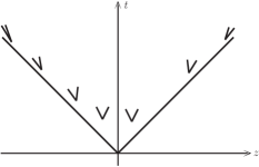
Figure 1: String model Artru (1983); Andersson et al. (1983) for hadronization of quark-antiquark pair in $e^{+}e^{-}$ annihilation, pictured in space-time. A string (or flux tube) is created between the outgoing quark and antiquark. Quark-antiquark pairs are created in the color field in the flux tube, and then combine into color singlet hadrons. The formation of the pairs occurs dominantly near a space-like hyperbola an invariant distance of order 1 $\textrm{fm}/c$ to the future of the approximately trajectories of the original quark and antiquark.

General features of string models include the chain decay ansatz, independent fragmentation, and an iterative scheme for generating final state hadrons Field and Feynman (1978). However, these classic hadronization models leave certain interesting issues, notably hadronization of polarized partons, unaddressed. This has led to recent proposals for extending hadronization models to include spin effects Kerbizi et al. (2017); Matevosyan et al. (2017); Bentz et al. (2016); Kerbizi et al. (2018).

A second background area to our work stems from the experimental observation that the particles observed in the final states of jets are approximately uniformly distributed in rapidity, e.g., Adolph et al. (2015), with the number of hadrons per unit rapidity depending weakly on the high-energy scale $Q$ or $\sqrt{s}$.

In the case of soft/minimum-bias hadron-hadron collisions, a simple and natural initial candidate model in Feynman-graph form is a multiperipheral model (MPM) Eden et al. (1966). Applied to $e^{+}e^{-}$ annihilation, using the structure of the MPM would give Fig. 2. Here, a quark-antiquark pair is generated from a virtual photon; the quark and antiquark go outwards. In the Feynman graph, the quark line is formed into a loop, and the hadrons are generated along that line, at momentum-conserving quark-hadron-quark vertices (which should be effective vertices in QCD). Because the line exchanged in the vertical channel is of a spin-half field, a single graph of fixed order is power suppressed as $Q$ increases. But the typical number of particles produced is intended to increase with $Q$ proportionally to $\ln(Q^{2}/m^{2})$, and in a strong-coupling situation this allows the result to be unsuppressed. The core idea of the MPM is a hypothesis Kogut et al. (1973) that the relevant interactions only occur between quanta with nearby kinematics.

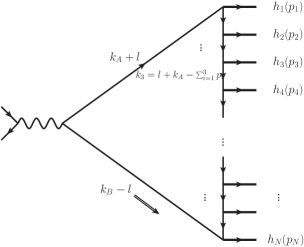
Figure 2: Elementary multiperipheral model for hadronization of quark-antiquark pair in $e^{+}e^{-}$ annihilation.

We emphasize the MPM because it corresponds to graphical structures that appear to be used in the work on polarized event generators Kerbizi et al. (2017); Matevosyan et al. (2017); Bentz et al. (2016); Kerbizi et al. (2018). In the case of the work by Artru, Kerbizi and collaborators Artru (2010); Artru and Belghobsi (2013); Artru (2012); Kerbizi et al. (2018), MPM graphs are explicitly given. In the case of Matevosyan et al. Matevosyan et al. (2017), the connection is less direct. They present their work as involving a sequence of splitting vertices, and in earlier work from the same group, Bentz et al. (2016) and especially Ito et al. (2009), the splitting vertices are treated as vertices in an effective theory. Assembling the vertices to make a model for the amplitude for the whole process gives MPM graphs. In both cases, these appearances are misleading.

In this paper, we first show that taking the MPM, Fig. 2, literally does not work. We show that the loop momentum can be deformed out of the intended region of kinematics into a region where short-distance pQCD physics is valid and the model, with its effective non-perturbative vertices is invalid. We then show that a motivated, minimal modification that does work is Fig. 3 with extra gluon lines; this matches both cluster hadronization and models of the Lund-string type, but now in Feynman-graph form. We will point out that models of this form could be considered a MPM, but with the quark-quark-hadron vertices and the associated connecting quark lines no longer being momentum conserving. Instead they should be considered as absorbing energy and momentum from the color flux tube. This dramatically changes the space-time structure.

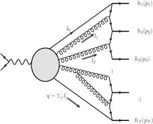
Figure 3: Modified multiperipheral model. It is modified from Fig. 2 by allowance for the emission of gluons. Note that the gluons may arise not only directly from the initial quark and antiquark lines but also, for example, from a splitting, as shown.

Consequently, the interpretation of apparently MPM-like structures in work on hadronization like Refs. Kerbizi et al. (2017); Matevosyan et al. (2017); Bentz et al. (2016); Kerbizi et al. (2018) must be modified to match string physics. Careful examination of these papers shows that this is indeed the case: Implementation of the kinematics of multiple splitting involves momentum non-conservation at the level of MPM graphs that corresponds to implementations of a string model.

Many elements of our work can be found in the literature, e.g., a graph like Fig. 3 for cluster hadronization. Just before QCD was formulated, Kogut, Sinclair, and Susskind Kogut et al. (1973) showed that multi-peripheral models cannot be applicable to hadronization in deep-inelastic scattering and $e^{+}e^{-}$ annihilation. Shortly afterwards, Casher, Kogut, and Susskind Casher et al. (1973, 1974), still before the advent of QCD, proposed what can now be called a string model. Our argument is a modernized version of those old arguments taking account of the much better knowledge we now have of QCD, and putting it in a new context.

The importance of formulating a hadronization model in terms of Feynman graphs (with effective vertices and propagators) is that it automatically obeys general principles of quantum mechanics and quantum field theory, of causality and of Lorentz invariance. They are natural arenas for consistently incorporating spin effects, especially with entangled spin states, which are hard to formulate purely semi-classically.

There is interesting work on effective field theory for chiral symmetry breaking Schweitzer et al. (2013). A better understanding of the imperatives of Feynman graph implementations of hadronization should lead to suggestions as to appropriate ways of applying the chiral models to hadronization.

II The elementary MPM

II.1 Basic Setup

Consider the graph shown in Fig. 2, as a possible model for production of hadronic final states in $e^{+}e^{-}$ annihilation. In accordance with data, we assume that a small number of particles (around three pions) is produced per unit rapidity, and with a limited transverse momentum all with respect to a jet axis (e.g., the thrust axis). The typical transverse momentum is perhaps 0.3 or 0.4 GeV.

We will work in a center-of-mass frame, and label the particles in order of rapidity along the jet axis. To define the $z$-axis, we choose hadron 1 to have zero transverse momentum and positive rapidity. Let the center-of-mass energy be $Q$. In light-front coordinates $(+,-,T)$, the virtual photon’s momentum is $q=(Q/\sqrt{2},Q/\sqrt{2},0_{T})$. Then we write the hadron momenta in terms of rapidity and transverse momentum:

$$p_{j}=\left(\frac{E_{j,T}}{\sqrt{2}}e^{y_{j}},\frac{E_{j,T}}{\sqrt{2}}e^{-y_{j}},\boldsymbol{p}_{j,T}\right),$$ (1)

where $E_{j,T}=\sqrt{p_{j,T}^{2}+m_{h}^{2}}$ and $m_{h}$ is the mass of the hadron. We have chosen $\boldsymbol{p}_{1,T}=0$. The momenta must obey momentum conservation: $\sum_{j=1}^{N}p_{j}=q$.

Given the assumptions of the model, a rough estimate of the hadron rapidities is given by

$$y_{j}\sim\frac{(N+1)-2j}{N-1}\ln\frac{Q}{m},$$ (2)

with the number of produced particles $N$ being approximately proportional to $\ln(Q^{2}/m^{2})$, with a coefficient of around 3, as already mentioned. (The coefficient could be rather less if the primary hadrons are mostly vector mesons instead of pions.)

For the purposes of the model, we assume that the internal loop line of Fig. 2 is for a quark, and that the hadrons are pions. But we will not use that assumption in any detail, since our concern is only with analytic properties, as determined by propagator denominators.

We define the origin of the loop momentum $l$ by writing the quark momenta from the electromagnetic vertex as $k_{A}+l$ and $k_{B}-l$, and defining

$$k_{A}=(Q/\sqrt{2},0,\boldsymbol{0}_{T}),\qquad k_{B}=(0,Q/\sqrt{2},\boldsymbol{0}_{T}),$$ (3)

which would be the quark and antiquark momenta if they were free and massless. Thus $l$ parameterizes the deviation of quark kinematics from parton-model values.

The momentum $k_{j}$ of the line between hadron $j$ and hadron $j+1$ is

$$k_{j}={} l+k_{A}-\sum_{i=1}^{j}p_{i}$$

$$={} l-k_{B}+\sum_{i=j+1}^{N}p_{i}.$$ (4)

Hence

$$k_{j}^{+}=l^{+}+\sum_{i=j+1}^{N}p_{i}^{+}~{}=~{}l^{+}+\Theta(me^{y_{j}})$$ (5)

and

$$k_{j}^{-}=l^{-}-\sum_{i=1}^{j}p_{i}^{-}~{}=~{}l^{-}-\Theta(me^{-y_{j}}).$$ (6)

In the last term in each equation, estimates are given with the aid of Knuth’s notation Knuth (1976) $\Theta(\dots)$ rather than the conventional order notation $O(\dots)$ to emphasize that the estimates are to within a finite factor. The usual “big $O$” notation would allow the actual result to be arbitrarily much smaller, which is not the case here. The estimates arise as follows: Because of the approximately uniform distribution of hadrons in rapidity, the sum in the equations is of an approximately geometrical series. Then the sums are dominated by the few terms whose index $i$ is nearest to $j$.

In analyzing the properties of the graph, we find it useful to consider first a baseline case given by $l=0$. The power counting for all lines, i.e., the sizes of their propagator denominators is then established by the above estimates. Each $k_{j}^{+}$ is strictly positive and each $k_{j}^{-}$ is strictly negative. This implies that the hadrons get their (mostly large) plus-momentum component from the upper quark line, and their minus momentum from the lower line. These conditions, and the sizes calculated, ensure that the virtualities of all the lines are of order $\Theta(m^{2})$, as is appropriate for a model of non-perturbative physics in QCD.

II.2 Integral over loop momentum $l$

Within the above description, the virtualities in the graph in Fig. 2 appear to be consistent with what one might expect for a model of non-perturbative physics, at least if $l=0$. However, $l$ is an integration variable.

Consider the process as having evolution in space-time from a quark-antiquark pair at short distances to a hadronic state at large distance. Then the conversion to hadrons occurs with unit probability. So the power law for making the quark-antiquark pair is the same as power counting for the full $e^{+}e^{-}\to\text{hadrons}$ cross section. That is, hadronization is a leading power effect. This also implies that the size of the non-perturbative effective quark-quark-hadron vertex must be such as to self-consistently give exactly the unit probability of hadronization.

Furthermore, for the MPM to implement the intended non-perturbative physics, $k_{A}+l$ and $k_{B}-l$ must have a normal non-perturbative virtuality,

$$(k_{A}+l)^{2}=\Theta(m^{2})\,,\qquad(k_{B}-l)^{2}=\Theta(m^{2})\,.$$ (7)

This also indicates that hadronization occurs long after the hard vertex.

If the integral were to stay in the region relevant for the assumed non-perturbative physics, then the transverse components of $l$ would be $\Theta(m)$, while the longitudinal components would be $\Theta(m^{2}/Q)$, i.e., $l$ would be in the Glauber region:

$$l=\left(\Theta\left(\frac{m^{2}}{Q}\right),\Theta\left(\frac{m^{2}}{Q}\right),\Theta(\boldsymbol{m}_{T})\right)\,.$$ (8)

This is simply because the virtualities of the $k_{A}+l$ and $k_{B}-l$ lines are:

$$(k_{A}+l)^{2}=2k_{A}^{+}l^{-}+l^{2}\,,\qquad(k_{B}-l)^{2}=-2k_{B}^{-}l^{+}+l^{2}\,,$$ (9)

and $k_{A}^{+}$ and $k_{B}^{-}$ are of order $Q$. If, however, $l$ is merely normal-soft (i.e., $l=(O(m),O(m),O(\boldsymbol{m}_{T}))$) then

$$(k_{A}+l)^{2}=\Theta\left(mQ\right)\,,\qquad(k_{B}-l)^{2}=\Theta\left(mQ\right)\,.$$ (10)

These are far off-shell, and therefore in a relatively short-distance region where standard weak coupling pQCD physics applies.

We will now show that we can apply a contour deformation that takes the integration out of the Glauber region, so that $l$ is at least soft and Eq. (10) is fulfilled. This is a standard result in the theory of factorization, but the detailed demonstration is slightly modified. The modification takes care of the fact that we have an array of hadrons filling in a rapidity range with no big gaps, whereas the usual arguments in factorization theory have configurations only with widely separated momenta.

To exhibit the contour deformation conveniently, we write each $k_{j}$ in the form $q_{j}+l$, where $q_{j}$ is the value obtained by computing $k_{j}$ from the external momenta when $l=0$, i.e.,

$$q_{j}=k_{A}-\sum_{i=1}^{j}p_{i}=-k_{B}+\sum_{i=j+1}^{N}p_{i}.$$ (11)

We deform the contour by adding an imaginary part to $l^{\pm}$:

$$l^{+}=l_{R}^{+}-i\Delta(l_{R}),\qquad l^{-}=l_{R}^{-}+i\Delta(l_{R}),$$ (12)

where $l_{R}^{\pm}$ are the real parts. The deformation is implemented by increasing the real number $\Delta$ from zero to a positive value. In general, we will allow $\Delta$ to depend on $l_{R}$, and we can also allow a different imaginary part of the two components of $l$. But initially, for use in the Glauber region, we will assume the 2 imaginary parts to be approximately equal and constant. Once $l_{R}^{\pm}$ is well outside the Glauber region, different amounts of deformation are allowed than in the Glauber region. But here we are only concerned with the deformation in the Glauber region, since that is the region in which the MPM is intended to be applied as a useful approximation to non-perturbative strong interactions.

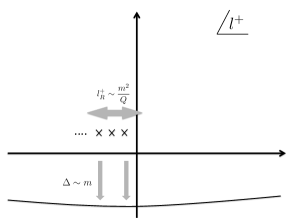
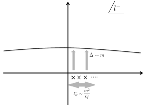
Figure 4: Singularity structure and contour deformations on $l^{+}$ and $l^{-}$ when $l$ is in the Glauber region ($|l^{+}l^{-}|\ll m^{2}$). On the deformed contour, some propagators are off-shell by order $\Theta(mQ)$—see Eqs. (15)–(17).

The denominator $k_{j}^{2}-m_{q}^{2}+i\epsilon=(q_{j}+l)^{2}-m_{q}^{2}+i\epsilon$ is

$$2(q_{j}^{+}+l^{+})(q_{j}^{-}+l^{-})-(\boldsymbol{q}_{j,T}+\boldsymbol{l}_{T})^{2}-m_{q}^{2}+i\epsilon,$$ (13)

whose real part is

$$2(q_{j}^{+}+l_{R}^{+})(q_{j}^{-}+l_{R}^{-})-(\boldsymbol{q}_{j,T}+\boldsymbol{l}_{T})^{2}-m_{q}^{2}+2\Delta^{2},$$ (14)

and whose imaginary part is

$$\epsilon+2(q_{j}^{+}-q_{j}^{-}+l_{R}^{+}-l_{R}^{-})\Delta\\ =\epsilon+2\left[\Theta(m\cosh(y_{j}))+l_{R}^{+}-l_{R}^{-}\right]\Delta,$$ (15)

given the estimates of $q_{j}^{\pm}$ that follow from (5) and (6). Also, the imaginary parts of the propagator denominators $(k_{A}+l)^{2}-m^{2}+i\epsilon$ and $(k_{B}-l)^{2}-m^{2}+i\epsilon$ are, respectively,

$$2\Delta\left(k_{A}^{+}-l^{+}_{R}+l_{R}^{-}\right)+\epsilon {}=2\Delta\left(\Theta(Q)-l_{R}^{+}+l_{R}^{-}\right)\,,$$ (16)

$$2\Delta\left(k_{B}^{-}-l^{+}_{R}+l_{R}^{-}\right)+\epsilon {}=2\Delta\left(\Theta(Q)-l_{R}^{+}+l_{R}^{-}\right)\,.$$ (17)

When $l_{R}^{\pm}$ are both smaller in size than $m$, as in the Glauber region, the imaginary part of every denominator is positive, so we have a successful deformation.

In the integration over $l_{R}$, once $l_{R}^{+}$ or $l_{R}^{-}$ gets to be bigger than order $m$ in size (and negative or positive, respectively), the imaginary part no longer retains its sign. For these larger values of $l_{R}^{\pm}$, a different deformation is needed; this traps the integral over $l^{\pm}$ in a region where the two components are of order $m$. But this is a region far beyond where the MPM was intended to be appropriate, for at least one quark line goes far off-shell, with a virtuality of order $Qm$ or more.

When $l_{R}^{\pm}$ is smaller than $m$, and especially much smaller, the allowed deformation enables us to get an imaginary part for $l^{\pm}$ that is of order $m$, by taking $\Delta$ of order $m$. It therefore follows that everywhere on the (deformed) integration contour, at least one of the longitudinal components of $l$ is at least of order $m$, and that we have propagators that are far off-shell, with virtuality of order $Qm$. (See Fig. 4.)

It might be naturally supposed that a model for non-perturbative physics would have some appropriate cut offs to remove any contribution from far off-shell propagators. But the cut offs should still obey standard relativistic causal and analytic properties. Therefore we can still deform out of the Glauber region into a region where the model is inappropriate.

Notice that most of the other quark lines also go far off-shell, since on the deformed contour $(q_{j}+l)^{2}-m_{q}^{2}=\Theta(m^{2}\cosh y_{j})$. Only the propagators for the low rapidity lines stay at low virtuality. Thus we get a strong suppression of the graph, compared with the power-counting estimate obtained from the power-counting that would be appropriate for the Glauber region.

It follows from the above arguments that the unadorned MPM does not adequately model the phenomena that it was intended to describe.

Note that this objection does not apply to the MPM applied to soft hadron-hadron collisions. To allow the contour deformation we needed a loop momentum that circulated through the hard scattering vertex; but a relevant loop does not exist in the case of hadron-hadron scattering.

III String-like MPM

In reality, a gluon field is created between the outgoing quark-antiquark pair. To allow for this, and for the creation of quark antiquark pairs in the gluon field, a simple model has the structure of Fig. 3. Here gluons are emitted from the quark and antiquark, and then we have attached one gluon to each of what in the MPM were quark lines joining neighboring hadrons. We will show that the integration is trapped in a region where the explicitly shown lines in Fig. 3 all have virtuality of order $m^{2}$. We will also show that in this region there is a radical change in the directions of the flow of longitudinal momentum on these quark lines, compared with the simple MPM. The quark lines are given different arrows than in the MPM; this is a mnemonic to indicate an important flow of positive components of momentum that is very different than in the simple MPM. There will remain lines that are far off shell, but these are in the shaded blob in Fig. 3.

To get these results, it is not necessary that exactly one gluon attach to each quark-line segment between hadrons; our results will apply also if multiple gluons attach to a segment, or if not too high a proportion of the segments have no gluon. The particular case in Fig. 3, with one gluon per segment, simply provides one specific case to illustrate the principles.

It should be observed that not only can the diagrammatic structure of Fig. 3 be considered as implementing the string model, but that it is also related to a diagrammatic formulation of the cluster-hadronization model Corcella et al. (2001); Bahr et al. (2008). Cluster hadronization is the other major hadronization model used in Monte-Carlo event generators.

A possible set of $N$ independent loop variables are the momentum of the upper quark, $l_{0}$, and the momentum $l_{j}$ of each of the $N-1$ gluon lines that connect to the (now modified) multiperipheral ladder. In accordance with the general features of the hadron kinematics, we assume that transverse momenta of these lines are of order $m$, and that the rapidity of $l_{j}$ is similar to the rapidity $y_{j}$ of a hadron near where it connects. That is, each gluon connects to a part of the ladder with similar rapidity to that of the gluon. These assumptions are appropriate to the non-perturbative physics we wish to model. We will term this region of kinematics the canonical region for the model. Integration outside the canonical region puts some propagators in the ladder much further off shell than $m^{2}$ and corresponds to different physics. The important issue is now to determine whether or not the integration is trapped in the canonical region, and we will find that it is indeed trapped.

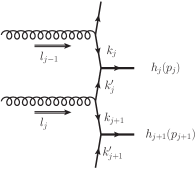
Figure 5: Component of string-like MPM.

We label the quark-line momenta as follows: $k_{j}$ is the momentum entering the vertex for hadron $j$ from above, and $k^{\prime}_{j}$ is the momentum entering from below — Fig. 5. By momentum conservation,

$$p_{j} =k_{j}+k^{\prime}_{j};\qquad 1<j<N$$ (18)

$$l_{j} =k^{\prime}_{j}+k_{j+1};\qquad 0<j<N$$ (19)

$$p_{1} =l_{0}+k_{1}^{\prime}$$ (20)

$$p_{N} =l_{N}+k_{N}\,,$$ (21)

where

$$l_{N}:=q-\sum_{j=0}^{N-1}l_{j}\,.$$ (22)

To further analyze the kinematics of the canonical region and to locate the conditions for the integration to be trapped there, we find it useful to change variables. We define fractional momentum variables at each quark-hadron vertex by:

$$x_{j}=k_{j}^{+}/p_{j}^{+};\qquad 1<j\leq N\,,$$ (23)

$$y_{j}={k^{\prime}}_{j}^{-}/p_{j}^{-};\qquad 1\leq j<N\,.$$ (24)

(The use of $k^{\prime}_{j}$ instead of $k_{j}$ in the second equation is to give a kind of symmetry under exchange of the roles of the initial quark and antiquark.) We define $x_{1}$ and $y_{N}$ by writing

$$l_{0}^{+}=x_{1}p_{1}^{+},\qquad l_{N}^{-}=q^{-}-\sum_{j=0}^{N-1}l_{j}^{-}=y_{N}p_{N}^{-}\,.$$ (25)

For the middle hadrons, $1<j<N$,

$$k_{j}^{+}=x_{j}p_{j}^{+},\quad k_{j}^{-}=(1-y_{j})p_{j}^{-},$$ (26)

$${k^{\prime}}_{j}^{+}=(1-x_{j})p_{j}^{+},\quad{k^{\prime}}_{j}^{-}=y_{j}p_{j}^{-},$$ (27)

and hence

$$l_{j}^{+}={} (1-x_{j})p_{j}^{+}+x_{j+1}p_{j+1}^{+},$$ (28)

$$l_{j}^{-}={} y_{j}p_{j}^{-}+(1-y_{j+1})p_{j+1}^{-},$$ (29)

while for $j=1$ and $j=N$, we have

$${k^{\prime}}_{1}^{+} =p_{1}^{+}-l_{0}^{+}=(1-x_{1})p_{1}^{+}; {k^{\prime}}_{1}^{-} =y_{1}p_{1}^{-}$$ (30)

$$k_{N}^{+} =x_{N}p_{N}^{+}; k_{N}^{-} =(1-y_{N})p_{N}^{-}\,.$$ (31)

(Note that there is no $k_{1}$ and no $k^{\prime}_{N}$.)

The momentum on the bottom quark line has plus component

$$l_{N}^{+}=q^{+}-\sum_{j=0}^{N-1}l_{j}^{+}={} p_{N}^{+}(1-x_{N})\,,$$ (32)

while the momentum of the top quark line has minus component

$$l_{0}^{-}=p_{1}^{-}(1-y_{1})\,.$$ (33)

The integration over the longitudinal components of the $l_{j}$ can be changed to integration over $x_{j}$ and $y_{j}$ with a simple Jacobian:

$$\prod_{j=0}^{N-1}(dl_{j}^{+}dl_{j}^{-})={} \prod_{j=1}^{N}(p_{j}^{+}p_{j}^{-})\prod_{j=1}^{N}(dx_{j}dy_{j})$$

$$={} \prod_{j=1}^{N}\left(\frac{E_{j,T}^{2}}{2}\right)\prod_{j=1}^{N}(dx_{j}dy_{j}).$$ (34)

As in the previous section, we use the term “canonical region” to refer to the momentum region that is consistent with the spacetime picture of hadronization. Thus, in the canonical region, Eqs. (25)–(33) mean that all the transverse momenta are of order $m$ and the $x_{j}$ and $y_{j}$ variables of order unity, and hence all the propagator denominators are of order $m^{2}$.

What we would mean if the integration were not trapped would be the following: There would be an allowed contour deformation such that everywhere on the contour at least one of the quark lines shown in Fig. 3 is much further off-shell than order $m^{2}$. We will find that in fact no such deformation is possible.

To specify an allowed deformation, we parameterize the surface of integration by the real parts of the values of the integration variables. We restrict our attention to the longitudinal momentum components, and work in terms of the fractional momenta $x_{j}$ and $y_{j}$. We use a real value $\lambda$ taking values in the range $0\leq\lambda\leq 1$ to parameterize the deformation starting from real momenta. We therefore write

$$x_{j} =x_{R,j}+i\lambda x_{I,j}(x_{R},y_{R}),$$ (35)

$$y_{j} =y_{R,j}+i\lambda y_{I,j}(x_{R},y_{R}).$$ (36)

By Cauchy’s theorem (generalized to multiple variables), the value of the integral is independent of $\lambda$ provided that the deformation is allowed, i.e., that no poles are crossed by the contour when $\lambda$ is increased from 0 to 1. There must be inserted in the integral a factor of the Jacobian for the transformation of variables from $x_{R,j}$ and $y_{R,j}$ to the complex variables $x_{j}$ and $y_{j}$.

Let us consider the region of integration where $x_{R}$ and $y_{R}$ are between $0$ and $1$. Then, from Eqs. (25)–(33), the contour of integration passes through the canonical region if $\lambda=0$. We will show that the integral is trapped in this region, and to do this we must show that there exists no choice of $x_{I,j}(x_{R},y_{R})$ and $y_{I,j}(x_{R},y_{R})$ such that we can increase $\lambda$ from 0 to 1, without crossing any poles, and such that the deformations obey $x_{I,j}\gg 1$ and $y_{I,j}\gg 1$ for at least some values of $j$. If such a deformation were to exist it would take the integration outside the canonical region. We will also require that the sizes of the derivatives, $|\partial x_{I,j}/\partial x_{R,k}|$ etc all stay bounded, say below 1, so that strongly varying structures in the imaginary parts don’t exist, and the Jacobian remains of order unity.

There do indeed exist non-trivial allowed deformations, but these all have $x_{I,j}$ and $y_{I,j}$ of order unity at most, and therefore stay in the canonical region.

Consider the relevant denominators:

$$k_{j}^{2}-m_{q}^{2}+i\epsilon={} 2x_{j}p_{j}^{+}(1-y_{j})p_{j}^{-}-k_{j,T}^{2}-m_{q}^{2}+i\epsilon$$

$$={} E_{j,T}^{2}x_{j}(1-y_{j})-k_{j,T}^{2}-m_{q}^{2}+i\epsilon,$$ (37)

$${k^{\prime}}_{j}^{2}-m_{q}^{2}+i\epsilon={} 2(1-x_{j})p_{j}^{+}y_{j}p_{j}^{-}-{k^{\prime}}_{j,T}^{2}-m_{q}^{2}+i\epsilon$$

$$={} E_{j,T}^{2}(1-x_{j})y_{j}-{k^{\prime}}_{j,T}^{2}-m_{q}^{2}+i\epsilon,$$ (38)

$$l_{j}^{2}-m_{g}^{2}+i\epsilon={} 2[(1-x_{j})p_{j}^{+}+x_{j+1}p_{j+1}^{+}]\times$$

$$\times[y_{j}p_{j}^{-}+(1-y_{j+1})p_{j+1}^{-}]-l_{j,T}^{2}-m_{g}^{2}+i\epsilon.$$ (39)

(Here, $m_{g}$ is a mass scale of order $\Lambda_{\rm QCD}^{2}$ representing the effects of confinement in cutting off soft gluons.) The transverse momenta and masses are of order $m$, as are the products of $p_{j}^{+}$ and $p_{j+1}^{+}$ with $p_{j}^{-}$ and $p_{j+1}^{-}$.

If we could find an allowed deformation out of the canonical region, at least one of the denominators would need to be much larger than $m^{2}$ on the deformed contour. As mentioned above, we are considering the part of the integration region where the real parts $x_{R,j}$ and $y_{R,j}$ are between zero and one. Then all of $x_{R,j}$, $1-x_{R,j}$, $y_{R,j}$, and $1-y_{R,j}$ are positive. Both of the momenta $k_{j}$ and $k^{\prime}_{j}$ are therefore future-pointing as regards both their (real) plus- and minus-components, which is unlike corresponding momenta in the pure MPM of Fig. 2.

Furthermore, to give an easy demonstration the non-existence of this hypothesized deformation, we restrict to the case that all of $x_{R,j}$, $1-x_{R,j}$, $y_{R,j}$, and $1-y_{R,j}$ are order unity rather than some being much less than unity.

The large size of $x_{j}$ or $y_{j}$ is achieved by the imaginary part, i.e., $|x_{I,j}|\gg 1$ and/or $|y_{I,j}|\gg 1$. The imaginary parts of the denominators for $k_{j}$ and $k^{\prime}_{j}$ are

$$\Im(k_{j}^{2}-m_{q}^{2}+i\epsilon)$$

$$\hskip 28.45274pt=\lambda E_{j,T}^{2}[x_{I,j}(1-y_{R,j})-y_{I,j}x_{R,j}]+\epsilon,$$ (40)

$$\Im({k^{\prime}}_{j}^{2}-m_{q}^{2}+i\epsilon)$$

$$\hskip 28.45274pt=\lambda E_{j,T}^{2}[-x_{I,j}y_{R,j}+y_{I,j}(1-x_{R,j})]+\epsilon.$$ (41)

Since $\epsilon>0$, then, starting at $\lambda=0$, to be able to deform off the real axis without crossing a pole the coefficients of $\lambda$ must be positive when the real parts of the momenta are at the corresponding pole. At the pole on the $k_{j}$ propagator, with $\lambda=0$, we have $1-y_{R,j}=(k_{j,T}^{2}+m_{q}^{2})/(E_{j,T}^{2}x_{R,j})$. So positivity of the imaginary part of the propagator for $k_{j}$, as we deform the contour off the real axis requires that

$$(k_{j,T}^{2}+m_{q}^{2})\frac{x_{I,j}}{x_{R,j}}-E_{j,T}^{2}x_{R,j}y_{I,j}$$ (42)

be positive for all $x_{R,j}$ between zero and one. Hence $x_{I,j}>0$ and $y_{I,j}<0$. But exactly the opposite condition applies to get a positive imaginary part for the denominator for the other line, $k^{\prime}_{j}$. That is, at the pole for $k^{\prime}_{j}$ with $\lambda=0$, we have $1-x_{R,j}=({k^{\prime}}_{j,T}^{2}+m_{q}^{2})/(E_{j,T}^{2}y_{R,j})$. The condition for doing a deformation without crossing a pole is

$$({k^{\prime}}_{j,T}^{2}+m_{q}^{2})\frac{y_{I,j}}{y_{R,j}}-E_{j,T}^{2}y_{R,j}x_{I,j}>0\,.$$ (43)

This requires $x_{I,j}<0$ and $y_{I,j}>0$. Thus, allowed deformations for $k_{j}$ lines clash with allowed deformations for $k^{\prime}_{j}$ lines. So no deformation far out of the canonical region is possible for any set of $x_{I,j}$ or $y_{I,j}$.

The poles on the two lines $k_{j}$ and ${k^{\prime}}_{j}$ are at different locations in $x_{j}$ and $y_{j}$. We could therefore imagine avoiding them by changing the sign of the imaginary part of one or more integration variables between the poles. But since to get a large denominator the imaginary part of the variable has to be much larger than unity, the derivative with respect to the real part would also be much larger than unity, which violates the smoothness requirement adopted earlier.

We have found that examination of the $k_{j}$ and $k^{\prime}_{j}$ denominators is sufficient to show that the integration is trapped in the canonical region, with the denominators being of order $m^{2}$. In this region, the denominators for the gluon lines $l_{j}$ are also of order $m^{2}$. In fact these denominators also participate in the trapping. For example, if we have the $x_{I,j}$ positive and the $y_{I,j}$ negative to avoid the poles of the $k_{j}$ lines, as above, then the imaginary part of the $l_{j}$ denominator (III) does not have a fixed sign, and so the hypothesized deformation is not allowed.

Notice that getting a situation where the contour is trapped in the canonical region depends on the gluons being able to inject appropriate amounts of momentum into the would-be multiperipheral ladder. Then about half the plus- and minus- momentum components on the quark lines are reversed in sign compared with the elementary MPM.

IV Discussion

We have shown that in the elementary MPM for non-perturbative hadronization in $e^{+}e^{-}$ annihilation, the loop integration can be deformed far out of the momentum region appropriate to its hypothesized validity. A minimal requirement for an appropriate non-perturbative model of a Feynman-graph kind, is that it incorporate the effects of gluon emission in a string-like way, as in Fig. 3.

There are dramatic differences in the directions of momentum flow and in the space-time structure between that graph and the elementary MPM Fig. 2. In the MPM, quark lines, like $k_{A}+l$, are far off-shell after the contour deformation. So the fastest hadrons are formed first. This is in complete contrast Casher et al. (1974) to string-like models, where the fastest hadrons are formed last, on an appropriate time-dilated scale.

The importance of these results is for the formulation and interpretation of models of non-perturbative hadronization of hard jets. For example, the successful string-inspired model of Refs. Kerbizi et al. (2017); Artru (2012, 2010); Artru and Belghobsi (2013) is formulated in terms of multiperipheral graphs. The use of a Feynman graph formulation allows the systematic and consistent incorporation of spin effects. This is in contrast to purely semi-classical formulations of a string hadronization, where the use of the ideas of classical, non-quantum physics makes it much harder to see how to incorporate the intrinsically quantum mechanical phenomenon of quark spin. The results in the present paper indicate that the graphs must be interpreted as containing momentum-non-conserving vertices or propagators in an external gluon field. The consequences can be seen in Ref. Kerbizi et al. (2018), where there is an explicit allowance for transfer of energy and momentum between the quarks and the string, with a non-trivial identification of the momentum to use in the vertices of the multi-peripheral graph.

The results in Ref. Matevosyan et al. (2017); Bentz et al. (2016) are developed from earlier work Ito et al. (2009) that used a chiral model of the Nambu-Jona-Lasinio (NJL) Nambu and Jona-Lasinio (1961a, b) type applied to a lowest order graph for fragmentation of a quark into a pion plus a quark. After iteration to apply to multiple splittings, such a model gives graphical structures like that of the MPM. Calculations such as those in Ito et al. (2009) applied to a splitting $q_{j}\to\pi_{j}+q_{j+1}$, have the final quark on-shell, and the initial quark off-shell. But to iterate Matevosyan et al. (2017) the splitting, the final quark, $q_{j+1}$ is changed to be off-shell. This is formulated according to the Field-Feynman structure; it amounts to a kind of momentum non-conservation appropriate to implementing a string model. Another useful resources is Ref. Accardi et al. (2010), which addresses the spacetime structure of hadronization in the Lund string model in Sec. 2.4. Such methods might help further clarify the relationship between Feynman graph structures and hadronization.

Chiral models can be argued to be useful as effective low-energy approximations to QCD. These models are important because they aim to capture the properties of QCD associated with chiral symmetry breaking. The results in this paper suggest an important direction for enhancing models such as the one in Ref. Schweitzer et al. (2013) to apply to high-energy dynamical processes like the non-perturbative hadronization of hard jets. This is to formulate the theories to apply to processes that occur in the background of an non-vacuum state that corresponds to a gluonic flux-tube. There are probably some useful tools to relate strings and field theory in the paper by Artru and Bowler (1988) on the quantization of the string by a sum-over-histories method.

Appendix A Estimate of number of particles per unit rapidity

In Ref. Braunschweig et al. (1990), the TASSO experiment reported results on the distribution of charged hadrons in jets in $e^{-}e^{-}$ annihilation at $Q$ between 14 and 44 GeV. In Table 9 are shown values for the normalized cross section $(1/\sigma_{\text{tot}})d\sigma/d\ln(1/x)$. Here $x=2p/Q$, where $p$ is the momentum of the detected particle; to a leading approximation, $x$ corresponds to the fragmentation variable $z$. We now roughly extract from this data the number of hadrons per unit rapidity in a jet.

For hadrons of high rapidity, Eq. (1) gives a corresponding $x$ value:

$$x=\frac{E_{j,T}}{Q}e^{y_{j}}.$$ (44)

Hence the rapidity distribution in fragmentation is given by $dN/dy=(1/2\sigma_{\text{tot}})d\sigma/d\ln(1/x)$. The extra factor of $1/2$ is to compensate the fact that the $x$ distribution gets a contribution from each jet. The most common particles in jets are pions. Isospin and charge conjugation symmetry show that the neutral pion fragmentation function in a $u$ or $d$ quark is half the charged pion fragmentation function: $f_{\pi^{0}/u}=(f_{\pi^{+}/u}+f_{\pi^{-}/u})/2$, etc. Thus the total hadronic number distribution is $3/2$ times the charged hadron distribution. Hence $dN^{\text{all}}/dy=(1/2\sigma_{\text{tot}})d\sigma^{\text{ch.}}/d\ln(1/x)$. In Table 9 of Ref. Braunschweig et al. (1990), the values of this quantity first increase as $\ln(1/x)$ is increased from 0 (which corresponds to $x=1$ or $z=1$). They reach a peak and then decrease. Now, once the rapidity is lower than a unit or two, it is not appropriate to apply the above approximations. So we take the peak value as the relevant one. Furthermore, as $Q$ increases, perturbative gluon emission becomes more important; this increases the hadron multiplicity beyond what it appears appropriate to attribute to purely non-perturbative QCD. So we take the peak in $(1/\sigma_{\text{tot}})d\sigma/d\ln(1/x)$ at $Q=14\,\mathrm{GeV}$ as the relevant one to estimate $dN/dy\simeq 3$. This is the number of hadrons per unit rapidity in the interior of the string.

References

- Sjöstrand (2016) T. Sjöstrand, “Status and developments of event generators,” Proceedings, 4th Large Hadron Collider Physics Conference (LHCP 2016): Lund, Sweden, June 13-18, 2016, PoS LHCP2016, 007 (2016), arXiv:1608.06425 [hep-ph] .
- Artru and Collins (1996) X. Artru and J. C. Collins, “Measuring transverse spin correlations by 4-particle correlations in ,” Z. Phys. C69, 277–286 (1996), arXiv:hep-ph/9504220 .
- Kerbizi et al. (2017) A. Kerbizi, X. Artru, Z. Belghobsi, F. Bradamante, A. Martin, and E. R. Salah, “Recursive Monte Carlo code for transversely polarized quark jet,” in 22nd International Symposium on Spin Physics (SPIN 2016) Urbana, IL, USA, September 25–30, 2016 (2017) arXiv:1701.08543 [hep-ph] .
- Matevosyan et al. (2017) H. H. Matevosyan, A. Kotzinian, and A. W. Thomas, “Monte Carlo implementation of polarized hadronization,” Phys. Rev. D95, 014021 (2017), arXiv:1610.05624 [hep-ph] .
- Bentz et al. (2016) W. Bentz, A. Kotzinian, H. H. Matevosyan, Y. Ninomiya, A. W. Thomas, and K. Yazaki, “Quark-jet model for transverse momentum dependent fragmentation functions,” Phys. Rev. D94, 034004 (2016), arXiv:1603.08333 [nucl-th] .
- Kerbizi et al. (2018) A. Kerbizi, X. Artru, Z. Belghobsi, F. Bradamante, and A. Martin, “Recursive model for the fragmentation of polarized quarks,” Phys. Rev. D97, 074010 (2018), arXiv:1802.00962 [hep-ph] .
- Adolph et al. (2015) C. Adolph et al. (COMPASS), “Collins and Sivers asymmetries in muonproduction of pions and kaons off transversely polarised protons,” Phys. Lett. B744, 250–259 (2015), arXiv:1408.4405 [hep-ex] .
- Artru (2012) X. Artru, “String fragmentation model with quark spin,” Proceedings, 3rd International Conference on Quantum Electrodynamics and Statistical Physics (QEDSP 2011): Kharkov, Ukraine, August 29-September 2, 2011, Prob. Atomic Sci. Technol. 2012N1, 173–178 (2012).
- Artru (2010) X. Artru, “Recursive fragmentation model with quark spin. application to quark polarimetry,” (2010), arXiv:1001.1061 [hep-ph] .
- Artru and Belghobsi (2013) X. Artru and Z. Belghobsi, “Theoretical considerations for a jet simulation with spin,” in XV Advanced Research Workshop on High Energy Spin Physics, edited by A. Efremov and S. Goloskokov (Dubna, Russia, 2013) pp. 33–40.
- Collins (2017) J. Collins, “Do fragmentation functions in factorization theorems correctly treat non-perturbative effects?” Proceedings, QCD Evolution Workshop (QCD 2016): Amsterdam, Netherlands, May 30-June 3, 2016, PoS QCDEV2016, 003 (2017), arXiv:1610.09994 [hep-ph] .
- Artru and Mennessier (1974) X. Artru and G. Mennessier, “String model and multiproduction,” Nucl. Phys. B70, 93–115 (1974).
- Field and Feynman (1978) R. D. Field and R. P. Feynman, “A parametrization of the properties of quark jets,” Nucl. Phys. B136, 1 (1978).
- Andersson et al. (1983) B. Andersson, G. Gustafson, G. Ingelman, and T. Sjostrand, “Parton fragmentation and string dynamics,” Phys. Rept. 97, 31–145 (1983).
- Artru (1983) X. Artru, “Classical string phenomenology. How strings work,” Phys. Rept. 97, 147–171 (1983).
- Andersson (1998) B. Andersson, The Lund Model (Cambridge University Press, Cambridge, 1998).
- Sjöstrand et al. (2006) T. Sjöstrand, S. Mrenna, and P. Z. Skands, “PYTHIA 6.4 physics and manual,” JHEP 05, 026 (2006), arXiv:hep-ph/0603175 .
- Sjöstrand et al. (2008) T. Sjöstrand, S. Mrenna, and P. Z. Skands, “A brief introduction to PYTHIA 8.1,” Comput. Phys. Commun. 178, 852–867 (2008), arXiv:0710.3820 [hep-ph] .
- Field and Wolfram (1983) R. D. Field and S. Wolfram, “A QCD Model for Annihilation,” Nucl. Phys. B213, 65–84 (1983).
- Webber (1984) B. R. Webber, “A QCD Model for Jet Fragmentation Including Soft Gluon Interference,” Nucl. Phys. B238, 492–528 (1984).
- Eden et al. (1966) R. J. Eden, P. V. Landshoff, D. I. Olive, and J. C. Polkinghorne, The Analytic S-matrix (Cambridge University Press, Cambridge, 1966).
- Kogut et al. (1973) J. B. Kogut, D. K. Sinclair, and L. Susskind, “Hadronic final states of deep-inelastic processes in simple quark-parton models,” Phys. Rev. D7, 3637–3657 (1973), [Erratum: Phys. Rev.D8,3709(1973)].
- Ito et al. (2009) T. Ito, W. Bentz, I. C. Cloet, A. W. Thomas, and K. Yazaki, “The NJL-jet model for quark fragmentation functions,” Phys. Rev. D80, 074008 (2009), arXiv:0906.5362 [nucl-th] .
- Casher et al. (1973) A. Casher, J. B. Kogut, and L. Susskind, “Vacuum polarization and the quark parton puzzle,” Phys. Rev. Lett. 31, 792–795 (1973).
- Casher et al. (1974) A. Casher, J. B. Kogut, and L. Susskind, “Vacuum polarization and the absence of free quarks,” Phys. Rev. D10, 732–745 (1974).
- Schweitzer et al. (2013) P. Schweitzer, M. Strikman, and C. Weiss, “Intrinsic transverse momentum and parton correlations from dynamical chiral symmetry breaking,” JHEP 1301, 163 (2013), arXiv:1210.1267 [hep-ph] .
- Braunschweig et al. (1990) W. Braunschweig et al. (TASSO), “Global jet properties at 14 GeV to 44 GeV center-of-mass energy in annihilation,” Z. Phys. C47, 187–198 (1990).
- Knuth (1976) D. E. Knuth, “Big omicron and big omega and big theta,” ACM SIGACT News 8, 18–24 (1976).
- Corcella et al. (2001) G. Corcella et al., “HERWIG 6.5: an event generator for hadron emission reactions with interfering gluons (including supersymmetric processes),” JHEP 01, 010 (2001), arXiv:hep-ph/0011363 .
- Bahr et al. (2008) M. Bahr et al., “Herwig++ physics and manual,” Eur. Phys. J. C58, 639–707 (2008), arXiv:0803.0883 [hep-ph] .
- Nambu and Jona-Lasinio (1961a) Y. Nambu and G. Jona-Lasinio, “Dynamical model of elementary particles based on an analogy with superconductivity. 1.” Phys. Rev. 122, 345–358 (1961a).
- Nambu and Jona-Lasinio (1961b) Y. Nambu and G. Jona-Lasinio, “Dynamical model of elementary particles based on an analogy with superconductivity. II,” Phys. Rev. 124, 246–254 (1961b).
- Accardi et al. (2010) A. Accardi, F. Arleo, W. K. Brooks, D. D’Enterria, and V. Muccifora, “Parton Propagation and Fragmentation in QCD Matter,” Riv. Nuovo Cim. 32, 439–553 (2010), arXiv:0907.3534 [nucl-th] .
- Artru and Bowler (1988) X. Artru and M. G. Bowler, “Quantization of the string fragmentation model,” Z. Phys. C37, 293 (1988).