OPARC: Optimal and Precise Array Response Control Algorithm – Part II: Multi-points
and Applications

Abstract

In this paper, the optimal and precise array response control (OPARC) algorithm proposed in Part I of this two paper series is extended from single point to multi-points. Two computationally attractive parameter determination approaches are provided to maximize the array gain under certain constraints. In addition, the applications of the multi-point OPARC algorithm to array signal processing are studied. It is applied to realize array pattern synthesis (including the general array case and the large array case), multi-constraint adaptive beamforming and quiescent pattern control, where an innovative concept of normalized covariance matrix loading (NCL) is proposed. Finally, simulation results are presented to validate the superiority and effectiveness of the multi-point OPARC algorithm.

I Introduction

In the companion paper [1], optimal and precise array response control (OPARC) algorithm was proposed and analyzed. OPARC provides a new mechanism to control array responses at a given set of angles, by simply assigning virtual interference one-by-one. The optimality (in the sense of array gain) of OPARC in each step is guaranteed. Nevertheless, OPARC only controls one point per step and may be inefficient if multiple points are needed to be precisely adjusted. Moreover, how to use the OPARC algorithm in practical cases (where real data commonly exists) remains.

This paper first extends the OPARC algorithm from single point response control per step to multi-point response control per step. Note that a multi-point accurate array response control (${\textrm{M}}{\textrm{A}}^{2}\textrm{RC}$) algorithm has been recently developed in [2]. Nevertheless, since it is built on the basis of the accurate array response control (${\textrm{A}}^{2}\textrm{RC}$) algorithm [3], the ${\textrm{M}}{\textrm{A}}^{2}\textrm{RC}$ suffers from the similar drawbacks to ${\textrm{A}}^{2}\textrm{RC}$, i.e., a solution is empirically adopted and hence a satisfactory performance cannot be always guaranteed as analyzed in details in [1]. In this paper, we first carry out a careful investigation on the change rule of the optimal beamformer when multiple virtual interferences are simultaneously assigned. Then, a generalized methodology of the weight vector update is observed and utilized for the realization of the multi-point array response control. Similar to the OPARC in [1], we formulate a constrained optimization problem such that the array response levels of multiple points can be optimally (in the sense of array gain) and precisely controlled. Then, two different solvers, by either taking advantage of the OPARC algorithm or employing the recently developed consensus alternating direction method of multipliers (C-ADMM) approach in [4], are provided to find an approximate solution of the established optimization problem. Note that since the OPARC in [1] only optimally controls the array response at one point in each step, it has a closed-form solution, while this is not the case for the multi-point OPARC in this paper. In other words, this paper does not cover [1]. The differences between the proposed multi-point OPARC and ${\textrm{M}}{\textrm{A}}^{2}\textrm{RC}$ are similar to those between OPARC and ${\textrm{A}}^{2}\textrm{RC}$ as described in [1] in details. Meanwhile, for the proposed multi-point OPARC, its applications to, such as, array pattern synthesis, multi-constraint adaptive beamforming and quiescent pattern control, are also presented as detailed below.

Application to Array Pattern Synthesis: Array pattern synthesis is a fundamental problem for radar, communication and remote sensing. Most of the existing pattern synthesis approaches, for instance, the global optimization based methods in [5, 6, 7], the convex programming (CP) methods in [8, 9, 10], and the adaptive array theory based method in [11], have no ability to precisely control the beampattern according to a given requirement. In this paper, the above shortcoming is overcome by synthesizing desirable patterns with the proposed multi-point OPARC algorithm. We start the synthesis procedure from the quiescent pattern, and iteratively adjust the responses of multiple angles to their desired levels. Simulation results show that it only requires a few steps of iteration to complete the syntheses of well-shaped beampatterns.

In addition to the consideration for a general array, large array pattern synthesis problem [12], where the existing methods consume a large amount of computing resources or even not work at all, is particularly discussed. We will see that the large array pattern synthesis can be readily realized with the multi-point OPARC algorithm, in a computationally attractive manner.

Application to Multi-constraint Adaptive Beamforming: Adaptive beamforming plays an important role in various application areas, since it enables us to receive a desired signal from a particular direction while it simultaneously blocks undesirable interferences. Multi-constraint adaptive beamforming, i.e., designing an adaptive beamformer with several fixed directional constraints, is a common strategy to improve the robustness of the adaptive beamformer, see [13, 14, 15] for example. The existing methods may cause distorted beampatterns, due to their imperfections on model building or parameter optimization. Based on the proposed multi-point OPARC algorithm, a new approach to multi-constraint adaptive beamforming is presented in this paper. We modify the traditional adaptive beamformer to make the prescribed amplitude constraints satisfied by utilizing the multi-point OPARC algorithm. In the proposed algorithm, the total signal-to-interference-plus-noise ratio (SINR) (taking both real interferences and assigned virtual interferences into consideration) is maximized, and the real unexpected components can be well rejected without leading to any undesirable pattern distortion. Inspired by this, a new concept of normalized covariance matrix loading (NCL), which can be regarded as a generalization of the conventional diagonal loading (DL) in [16, 17, 18], is developed. Moreover, NCL is also exploited to realize quiescent pattern control as introduced next.

Application to Quiescent Pattern Control: In brief, when an adaptive array operates in the presence of white noise only, the resultant adaptive beamformer is referred to as the quiescent weight vector, and the corresponding array response is termed as the quiescent pattern. As pointed out in [19], having overall low sidelobes is important to adaptive arrays and how to specify a quiescent response pattern is worthwhile investigating. Most of the existing quiescent pattern control methods [19, 20, 21] are established on the foundation of the linearly constrained minimum variance (LCMV) framework, where the unnecessary phase constraints of array response are implicitly imposed. In this paper, a simple yet effective quiescent pattern control algorithm is proposed. We synthesize a satisfactory deterministic pattern, i.e., the ultimate quiescent pattern, by adopting the multi-point OPARC algorithm, and meanwhile, collect the resulting virtual normalized covariance matrix (VCM) for later use. Under the real data circumstance, the quiescent pattern control is completed by conducting a simple NCL operator to the existed VCM, and the weight vector can be obtained accordingly.

This paper is organized as follows. The proposed multi-point OPARC algorithm is presented in Section II. The three applications of the multi-point OPARC are discussed in Section III. Representative experiments are carried out in Section IV and conclusions are drawn in Section V.

Notations: The same as [1], we use bold upper-case and lower-case letters to represent matrices and vectors, respectively. In particular, we use ${\bf I}$ to denote the identity matrix. $j\triangleq\sqrt{-1}$. $(\cdot)^{\mathop{\rm T}}$ and $(\cdot)^{\mathop{\rm H}}$ stand for the transpose and Hermitian transpose, respectively. $|\cdot|$ denotes the absolute value and $\|\cdot\|_{2}$ denotes the $l_{2}$ norm. We use $({\bf g})_{i}$ to stand for the $i$th element of vector ${\bf g}$. $\Re(\cdot)$ and $\Im(\cdot)$ denote the real and imaginary parts, respectively. $\oslash$ represents the element-wise division operator. We use ${\rm Diag}(\cdot)$ to stand for the diagonal matrix with the components of the input vector as the diagonal elements. $\mathbb{R}$ and $\mathbb{C}$ denote the sets of all real and all complex numbers, respectively. Finally, $\cup$ denotes the set union and ${\rm card}(\cdot)$ returns the number of elements in a set.

II Multi-point OPARC Algorithm

To present our multi-point OPARC algorithm, we first make a detailed analysis on the optimal weight vector.

II-A Multi-interference Optimal Beamformer

Consider an array with $N$ elements. The same as [1], the optimal weight vector:

$${\bf w}_{\rm opt}={\bf T}^{-1}_{n+i}{\bf a}(\theta_{0})$$ (1)

maximizes both the output signal-to-interference-plus-noise ratio (SINR) and the array gain of an array system, where SINR and array gain are defined, respectively, as [22]

$${\rm SINR}\triangleq\dfrac{{\sigma}^{2}_{s}|{\bf w}^{\mathop{\rm H}}{\bf a}(\theta_{0})|^{2}}{{\bf w}^{\mathop{\rm H}}{\bf R}_{n+i}{\bf w}},~{}~{}~{}G\triangleq\dfrac{|{\bf w}^{\mathop{\rm H}}{\bf a}(\theta_{0})|^{2}}{{\bf w}^{\mathop{\rm H}}{\bf T}_{n+i}{\bf w}}$$ (2)

where ${\bf a}(\theta)$ stands for the array steering vector:

$${\bf a}(\theta)=[g_{1}(\theta)e^{-j\omega\tau_{1}(\theta)},\cdots,g_{N}(\theta)e^{-j\omega\tau_{N}(\theta)}]^{\mathop{\rm T}}$$ (3)

where $g_{n}(\theta)$ denotes the pattern of the $n$th element, $\tau_{n}(\theta)$ is the time-delay between the $n$th element and the reference point, $n=1,\cdots,N$, $\omega$ denotes the operating frequency. In the above notations, $\theta_{0}$ is the beam axis, ${\bf R}_{n+i}$ denotes the $N\times N$ noise-plus-interference covariance matrix, ${\bf T}_{n+i}$ stands for the normalized covariance matrix satisfying

$${\bf T}_{n+i}=\frac{{\bf R}_{n+i}}{\sigma_{n}^{2}}={\bf I}+\sum_{l=1}^{Q}{\beta}_{l}{\bf a}(\theta_{l}){\bf a}^{\mathop{\rm H}}(\theta_{l})$$ (4)

where ${\beta}_{l}\triangleq{{\sigma}^{2}_{l}}/{{\sigma}^{2}_{n}}$ denotes the interference-to-noise ratio (INR), $Q$ is the number of interferences, ${\bf a}(\theta_{l})$ is the steering vector of the $l$th interference, ${\sigma}^{2}_{s}$, ${\sigma}^{2}_{n}$ and ${\sigma}^{2}_{l}$ stand for the powers of signal, noise and the $l$th interference, respectively. Note that $G$ in (2) represents the amplification factor of the input signal-to-noise ratio (SNR) ${\sigma_{s}^{2}}/{\sigma_{n}^{2}}$, and the criterion of array gain maximization is adopted to achieve the optimal weight vector.

$${\bf w}_{k,\star}={\bf w}_{k-1,{\star}}-{\bf T}^{-1}_{k-1}{\bf A}_{k}\left({\bf I}+{\bf\Sigma}_{k,\star}{\bf A}^{\mathop{\rm H}}_{k}{\bf T}^{-1}_{k-1}{\bf A}_{k}\right)^{-1}{\bf\Sigma}_{k,\star}{\bf A}^{\mathop{\rm H}}_{k}{\bf T}^{-1}_{k-1}{\bf a}(\theta_{0})$$ (15)

From (1)-(2), one can see that the optimal weight vector ${\bf w}_{\rm opt}$ depends on ${{\bf R}_{n+i}}$ or ${\bf T}_{n+i}$, which is normally data-dependent. For this reason, ${{\bf R}_{n+i}}$ or ${\bf T}_{n+i}$ may not be available if we need to design a data-independent array response pattern $L(\theta,\theta_{0})\triangleq{|{\bf w}^{\mathop{\rm H}}{\bf a}(\theta)|^{2}}\big{/}{|{\bf w}^{\mathop{\rm H}}{\bf a}(\theta_{0})|^{2}}$ that satisfies some specific requirements. In this case, for a given response design task, the concept of virtual normalized noise-plus-interference covariance matrix (VCM) was introduced in [1]. Moreover, it was shown in [1] that a VCM can be constructed by assigning suitable virtual interferences one-by-one. In this paper, for a given response control task, we assign multiple virtual interferences (instead of a single virtual interference) at one step, and study how the optimal weight vector in (1) changes.

We use induction to describe the problem. Suppose that we have already assigned interferences for $(k-1)$ times, the total number of interferences is accumulated as $Q_{k-1}$ and ${\bf T}_{k-1}$ denotes the total VCM upto the $(k-1)$th step. The corresponding optimal weight vector at the $(k-1)$th step is given by

$${\bf w}_{k-1}={\bf T}^{-1}_{k-1}{\bf a}(\theta_{0})$$ (5)

where the subscript $(\cdot)_{\rm opt}$ has been omitted for notational simplicity. Then, we carry out the $k$th step by assigning $M_{k}$ interferences from directions $\theta_{k,m}$ with INR to be ${\beta}_{k,m}$, $m=1,\cdots,M_{k}$, where $\theta_{k,m}$ are renamed from those $\theta_{l}$ in (4). Then,

$${\bf T}_{k} ={\bf T}_{k-1}+\sum_{m=1}^{M_{k}}{\beta}_{k,m}{\bf a}(\theta_{k,m}){\bf a}^{\mathop{\rm H}}(\theta_{k,m})$$

$$={\bf T}_{k-1}+{\bf A}_{k}{\bf\Sigma}_{k}{\bf A}^{\mathop{\rm H}}_{k}$$ (6)

where

$${\bf A}_{k} =[{\bf a}(\theta_{k,1}),\cdots,{\bf a}(\theta_{k,M_{k}})]$$ (7)

$${\bf\Sigma}_{k} ={\rm Diag}([{\beta_{k,1},\cdots,{\beta}_{k,M_{k}}}])$$ (8)

and ${\bf T}_{k}$ is the resulting VCM after implementing the $k$th step of the interference assigning. Clearly, if $M_{k}=1$, (II-A) degenerates to Eqn. (6) of [1], and the related discussions return to our previous work in [1]. To make the discussion meaningful, the matrix ${\bf A}_{k}$ in this paper is assumed to have a full column rank.

By applying the Generalized Woodbury Lemma [23] to (II-A), we obtain that

$${\bf T}^{-1}_{k} ={\bf T}^{-1}_{k-1}-$$

$$~{}~{}~{}{\bf T}^{-1}_{k-1}{\bf A}_{k}\left({\bf I}+{\bf\Sigma}_{k}{\bf A}^{\mathop{\rm H}}_{k}{\bf T}^{-1}_{k-1}{\bf A}_{k}\right)^{-1}{\bf\Sigma}_{k}{\bf A}^{\mathop{\rm H}}_{k}{\bf T}^{-1}_{k-1}.$$ (9)

Accordingly, the obtained optimal weight vector satisfies

$${\bf w}_{k}={\bf T}^{-1}_{k}{\bf a}(\theta_{0})={\bf w}_{k-1}+{\bf T}^{-1}_{k-1}{\bf A}_{k}{\bf h}_{k}$$ (10)

where ${\bf h}_{k}\in\mathbb{C}^{M_{k}}$ is

$${\bf h}_{k}=-\left({\bf I}+{\bf\Sigma}_{k}{\bf A}^{\mathop{\rm H}}_{k}{\bf T}^{-1}_{k-1}{\bf A}_{k}\right)^{-1}{\bf\Sigma}_{k}{\bf A}^{\mathop{\rm H}}_{k}{\bf T}^{-1}_{k-1}{\bf a}(\theta_{0}).$$ (11)

As shown in (10), the current optimal weight ${\bf w}_{k}$ is obtained by making a modification to the previous weight ${\bf w}_{k-1}$.

Recalling the adaptive array theory, the weight ${\bf w}_{k}$ performs optimally in maximizing the array gain $G_{k}$ defined as

$$G_{k}\triangleq{|{\bf w}^{\mathop{\rm H}}_{k}{\bf a}(\theta_{0})|^{2}}/{|{\bf w}^{\mathop{\rm H}}_{k}{\bf T}_{k}{\bf w}_{k}|}$$ (12)

although the response levels at $\theta_{k,m}$, $m=1,\cdots,M_{k}$, may not reach their expected values. To precisely adjust the array responses of $\theta_{k,m}$ to their desired levels $\rho_{k,m}$, the INRs $\beta_{k,m}$, $m=1,\cdots,M_{k}$, or equivalently the diagonal matrix ${\bf\Sigma}_{k}$, should be carefully selected. In the meantime, the array gain $G_{k}$ in (12) should be maximized. Note also that ${\bf h}_{k}$ in (11) acts as a mapping of ${{\bf\Sigma}_{k}}$, and we can express ${\bf\Sigma}_{k}$ by ${\bf h}_{k}$ as

$${\bf\Sigma}_{k}={\rm Diag}\left(-{\bf h}_{k}\oslash\left({\bf A}^{\mathop{\rm H}}_{k}{\bf T}^{-1}_{k-1}\left({\bf a}(\theta_{0})+{\bf A}_{k}{\bf h}_{k}\right)\right)\right).$$ (13)

From (11) and (13), one can see that ${\bf\Sigma}_{k}$ and ${\bf h}_{k}$ are one-one mapping. Therefore, the multi-point optimal and precise array response control (OPARC) can be realized by either finding a suitable ${\bf\Sigma}_{k}$ or selecting an appropriate ${\bf h}_{k}$.

II-B Multi-point OPARC Problem Formulation

Let us first formulate the multi-point OPARC by optimizing ${{\bf\Sigma}_{k}}$ as:

$$\max_{{\bf\Sigma}_{k}} ~{}~{}~{}G_{k}={|{\bf w}^{\mathop{\rm H}}_{k}{\bf a}(\theta_{0})|^{2}}/{|{\bf w}^{\mathop{\rm H}}_{k}{\bf T}_{k}{\bf w}_{k}|}$$ (14a)

$${\rm subject~{}to} ~{}~{}~{}L(\theta_{k,m},{\theta_{0}})={\rho}_{k,m},~{}m=1,\cdots,M_{k}$$ (14b)

$$~{}~{}~{}{\bf w}_{k}={\bf w}_{k-1,\star}+{\bf T}^{-1}_{k-1}{\bf A}_{k}{\bf h}_{k}$$ (14c)

where ${\bf w}_{k-1,\star}$ is the resultant weight vector of the $(k-1)$th step (we use the star symbol to indicate it as the ultimate selection of ${\bf w}_{k-1}$), the vector ${\bf h}_{k}$ is given by (11). Once the optimal ${\bf\Sigma}_{k,\star}$ has been obtained, we can express the ultimate weight vector ${\bf w}_{k,\star}$ as (15) on the top of this page. To find the solution of problem (14), an iterative method is first provided below.

II-C Iterative Approach

The OPARC algorithm, developed in the companion paper [1], is able to optimally and precisely adjust one-point response level at a time. Thus, we may apply it to the $M_{k}$-point OPARC problem (14) as follows. For a fixed $k>0$, we apply the OPARC algorithm for $M_{k}$ steps. In the $m$th step, OPARC is to realize $L(\theta_{k,m},\theta_{0})={\rho_{k,m}}$, $m=1,\cdots,M_{k}$. Unfortunately, OPARC brings inevitable pattern variations on the previous controlled angles as we have discussed in [1]. More specifically, the response levels of $\theta_{k,i}$, $i=1,\cdots,m-1$, vary after accurately controlling the response level of $\theta_{k,m}$ to its desired level $\rho_{k,m}$, $2\leq m\leq M_{k}$. To reduce the undesirable pattern variations on the pre-adjusted angles, we propose to iteratively apply the $M_{k}$-point OPARC for a number of times, until a certain termination criterion is met. A temporary variable ${\bf\Xi}={\bf T}_{k-1}$ and ${{\bf\Sigma}_{k}}={\bf 0}$ are taken as the initializations in the first iteration. Then, in each iteration, an $M_{k}$-step OPARC is carried out. More specifically, in the $m$th step, we adjust the response level of $\theta_{k,m}$ to be $\rho_{k,m}$, by calculating the INR of the newly assigned virtual interference at $\theta_{k,m}$, denoted as $\beta_{k,m,\star}$, $m=1,\cdots,M_{k}$, from Eqn. (38) of [1], and then update the associated VCM as ${\bf\Xi}={\bf\Xi}+{\beta}_{k,m,\star}{\bf a}(\theta_{k,m}){\bf a}^{\mathop{\rm H}}(\theta_{k,m})$. Once an iteration, i.e., an $M_{k}$-step OPARC, is completed, $\beta_{k,m,\star}$ is added to the $m$th diagonal element of ${{\bf\Sigma}_{k}}$, and then we set the resulting ${\bf\Xi}$ as the initial VCM in the next iteration. Note that ${\bf T}_{0}={\bf I}$.

Naturally, whether the response levels of the adjusted angles $\theta_{k,m}$, $m=1,\cdots,M_{k}$, are close enough to their desired levels can be a criterion to terminate the iteration of OPARC. However, this strategy needs to calculate all the intermediate weight vectors that may be computationally inefficient. To improve the computational efficiency, we propose to terminate the iteration of OPARC by examining whether the magnitudes of INRs of the newly assigned virtual interferences approximate enough to zero, since there is no need to assign virtual interferences if their values are small enough.

Finally, we summarize the above iterative solver of problem (14) in Algorithm 1, where ${\beta}_{\epsilon}$ stands for a small tolerance parameter. Note that ${\beta}_{k,m,\star}$ in Algorithm 1 is calculated with Eqn. (38) of [1]. In addition, we can express the ultimate ${\bf\Sigma}_{k,\star}$ as

$${\bf\Sigma}_{k,\star}={\rm Diag}([\bar{\beta}_{k,1,\star},\cdots,\bar{\beta}_{k,M_{k},\star}])$$ (16)

where $\bar{\beta}_{k,m,\star}$ represents the total INR of the virtual interference assigned at $\theta_{k,m}$ in the $k$th step, and equals to the summation of all ${\beta}_{k,m,\star}$’s of different iterations for a fixed $m=1,\cdots,M_{k}$. As discussed earlier, once the optimal ${\bf\Sigma}_{k,\star}$ has been obtained, we can use ${\bf\Sigma}_{k,\star}$ to obtain the VCM ${\bf T}_{k}$ by Eqn. (II-A), update ${\bf h}_{k}$ in (11) and (14c), and calculate ${\bf w}_{k,\star}$ by Eqn. (15). It shall be noted that an inverse of normalized covariance matrix is indispensable in determining $\beta_{k,m,\star}$’s by Eqn. (38) of [1]. This may lead to a high cost in memory or/and computation especially for a large array, although it may not need a large number of iterations.

Algorithm 1 Iterative Approach to Problem (14)

1:give ${\bf a}(\theta_{0})$, $\theta_{k,m}$, ${\rho_{k,m}}$, $m=1,\cdots,M_{k}$, and ${\bf A}_{k}$, set ${\beta}_{\epsilon}>0$, ${\beta}_{\rm MAX}>{\beta}_{\epsilon}$, ${\bf\Xi}={\bf T}_{k-1}$, ${\bf\Sigma}_{k}={\bf 0}$

2:while ${\beta}_{\rm MAX}>{\beta}_{\epsilon}$ do

3:     for $m=1,\cdots,M_{k}$ do

4:         calculate ${\beta}_{k,m,\star}$ from Eqn. (38) of [1], by setting $~{}~{}~{}~{}~{}~{}~{}~{}\!~{}~{}L(\theta_{k,m},\theta_{0})={\rho}_{k,m}$

5:         update VCM ${\bf\Xi}={\bf\Xi}+{\beta}_{k,m,\star}{\bf a}(\theta_{k,m}){\bf a}^{\mathop{\rm H}}(\theta_{k,m})$

6:     end for

7:     update ${\bf\Sigma}_{k}$ as ${\bf\Sigma}_{k}={\bf\Sigma}_{k}+{\rm Diag}([{\beta_{k,1,\star},\cdots,{\beta}_{k,M_{k},\star}}])$

8:     obtain $\beta_{\rm MAX}=\max\limits_{1\leq m\leq M_{k}}|{\beta}_{k,m,\star}|$

9:end while

10:obtain ${\bf\Sigma}_{k,\star}={\bf\Sigma}_{k}$

II-D C-ADMM Approach

We next propose another approach to solve problem (14). We first reformulate the original problem (14) as a quadratically constrained quadratic program (QCQP) problem. Then, the recently developed consensus-ADMM (C-ADMM) [4] approach is employed to find its solution.

II-D1 Problem Reformulation

Since ${\bf h}_{k}$ is a one-one mapping of ${\bf\Sigma}_{k}$, we can formulate the multi-point OPARC, i.e., problem (14), by finding ${\bf h}_{k}$ as

$$\max_{{\bf h}_{k}\in\mathbb{C}^{M_{k}}} ~{}~{}~{}G_{k}={|{\bf w}^{\mathop{\rm H}}_{k}{\bf a}(\theta_{0})|^{2}}/{|{\bf w}^{\mathop{\rm H}}_{k}{\bf T}_{k}{\bf w}_{k}|}$$ (17a)

$${\rm subject~{}to} ~{}~{}~{}L(\theta_{k,m},{\theta_{0}})={\rho}_{k,m},~{}m=1,\cdots,M_{k}$$ (17b)

$$~{}~{}~{}{\bf w}_{k}={\bf w}_{k-1,\star}+{\bf T}^{-1}_{k-1}{\bf A}_{k}{\bf h}_{k}.$$ (17c)

We substitute the constraint (17c) into $G_{k}$ and obtain

$$G^{2}_{k} =\big{|}{\bf a}^{\mathop{\rm H}}(\theta_{0})({\bf w}_{k-1,\star}+{\bf T}^{-1}_{k-1}{\bf A}_{k}{\bf h}_{k})\big{|}^{2}$$

$$=-{\bf h}^{\mathop{\rm H}}_{k}{\widetilde{\bf C}}{\bf h}_{k}+2{\Re}\left({\widetilde{\bf c}}^{\mathop{\rm H}}{\bf h}_{k}\right)+|{\bf a}^{\mathop{\rm H}}(\theta_{0}){\bf w}_{k-1,\star}|^{2}$$ (18)

where ${\bf w}_{k}={\bf T}^{-1}_{k}{\bf a}(\theta_{0})$ is used, ${\widetilde{\bf C}}$ and ${\widetilde{\bf c}}$ are defined as

$${\widetilde{\bf C}} \triangleq-({\bf T}^{-1}_{k-1}{\bf A}_{k})^{\mathop{\rm H}}{\bf a}(\theta_{0}){\bf a}^{\mathop{\rm H}}(\theta_{0}){\bf T}^{-1}_{k-1}{\bf A}_{k}\in{\mathbb{C}}^{{M_{k}}\times{M_{k}}}$$ (19a)

$${\widetilde{\bf c}} \triangleq({\bf T}^{-1}_{k-1}{\bf A}_{k})^{\mathop{\rm H}}{\bf a}(\theta_{0}){\bf a}^{\mathop{\rm H}}(\theta_{0}){\bf w}_{k-1,\star}\in{\mathbb{C}}^{M_{k}}.$$ (19b)

Since $|{\bf a}^{\mathop{\rm H}}(\theta_{0}){\bf w}_{k-1,\star}|^{2}$ is a constant, the maximization of $G_{k}$ is thus equivalent to the minimization of ${\bf h}^{\mathop{\rm H}}_{k}{\widetilde{\bf C}}{\bf h}_{k}-2{\Re}\left({\widetilde{\bf c}}^{\mathop{\rm H}}{\bf h}_{k}\right)$.

On the other hand, recalling the expression of $L(\theta,\theta_{0})$, we can rewrite the constraint (17b) as

$${\bf w}^{\mathop{\rm H}}_{k}{\bf S}_{k,m}{\bf w}_{k}=0,~{}m=1,\cdots,M_{k}$$ (20)

where ${\bf S}_{k,m}={\bf a}(\theta_{k,m}){\bf a}^{\mathop{\rm H}}(\theta_{k,m})-{\rho}_{k,m}{\bf a}(\theta_{0}){\bf a}^{\mathop{\rm H}}(\theta_{0})$. Substituting the constraint (17c) into (20), we have

$${\bf h}^{\mathop{\rm H}}_{k}{\widetilde{\bf D}_{m}}{\bf h}_{k}-2{\Re}({\widetilde{\bf d}}^{\mathop{\rm H}}_{m}{\bf h}_{k})={\alpha}_{m},~{}m=1,\cdots,M_{k}$$ (21)

where

$${\widetilde{\bf D}_{m}} =({\bf T}^{-1}_{k-1}{\bf A}_{k})^{\mathop{\rm H}}{\bf S}_{k,m}{\bf T}^{-1}_{k-1}{\bf A}_{k}\in{\mathbb{C}}^{{M_{k}}\times{M_{k}}}$$ (22a)

$${\widetilde{\bf d}_{m}} =-({\bf T}^{-1}_{k-1}{\bf A}_{k})^{\mathop{\rm H}}{\bf S}_{k,m}{\bf w}_{k-1,\star}\in{\mathbb{C}}^{M_{k}}$$ (22b)

$${\alpha}_{m} =-{\bf w}^{\mathop{\rm H}}_{k-1,\star}{\bf S}_{k,m}{\bf w}_{k-1,\star}\in{\mathbb{R}}.$$ (22c)

Thus, problem (17) can be reformulated as

$$\min_{{\bf h}_{k}} ~{}~{}~{}{\bf h}^{\mathop{\rm H}}_{k}{\widetilde{\bf C}}{\bf h}_{k}-2{\Re}\left({\widetilde{\bf c}}^{\mathop{\rm H}}{\bf h}_{k}\right)$$ (23a)

$${\rm subject~{}to} ~{}~{}~{}{\bf h}^{\mathop{\rm H}}_{k}{\widetilde{\bf D}_{m}}{\bf h}_{k}-2{\Re}({\widetilde{\bf d}}^{\mathop{\rm H}}_{m}{\bf h}_{k})={\alpha}_{m}$$ (23b)

$$~{}~{}~{}m=1,\cdots,M_{k}.$$

In the sequel, we adopt the newly developed C-ADMM approach [4] to solve problem (23).

II-D2 C-ADMM Solver

We first convert (23) into its real domain as

$$\min_{{\bf z}} ~{}~{}~{}{\bf z}^{\mathop{\rm T}}{\bf C}{\bf z}-2{\bf c}^{\mathop{\rm T}}{\bf z}$$ (24a)

$${\rm subject~{}to} ~{}~{}~{}{\bf z}^{\mathop{\rm T}}{\bf D}_{m}{\bf z}-2{\bf d}^{\mathop{\rm T}}_{m}{\bf z}={\alpha}_{m}$$ (24b)

$$~{}~{}~{}m=1,\cdots,M_{k}$$

where

$${\bf z} =\begin{bmatrix}{\Re}({\bf h}^{\mathop{\rm T}}_{k})&{\Im}({\bf h}^{\mathop{\rm T}}_{k})\end{bmatrix}^{\mathop{\rm T}}\in{\mathbb{R}}^{2{M_{k}}}$$ (25a)

$${\bf c} =\begin{bmatrix}{\Re}({\widetilde{\bf c}}^{\mathop{\rm T}})&{\Im}({\widetilde{\bf c}}^{\mathop{\rm T}})\end{bmatrix}^{\mathop{\rm T}}\in{\mathbb{R}}^{2{M_{k}}}$$ (25b)

$${\bf d}_{m} =\begin{bmatrix}{\Re}({\widetilde{\bf d}_{m}}^{\mathop{\rm T}})&{\Im}({\widetilde{\bf d}_{m}}^{\mathop{\rm T}})\end{bmatrix}^{\mathop{\rm T}}\in{\mathbb{R}}^{2{M_{k}}}$$ (25c)

$${\bf C} =\begin{bmatrix}{\Re}({\widetilde{\bf C}})&-{\Im}({\widetilde{\bf C}})\\ {\Im}({\widetilde{\bf C}})&{\Re}({\widetilde{\bf C}})\end{bmatrix}\in{\mathbb{R}}^{2{M_{k}}\times 2{M_{k}}}$$ (25d)

$${\bf D}_{m} =\begin{bmatrix}{\Re}({\widetilde{\bf D}_{m}})&-{\Im}({\widetilde{\bf D}_{m}})\\ {\Im}({\widetilde{\bf D}_{m}})&{\Re}({\widetilde{\bf D}_{m}})\end{bmatrix}\in{\mathbb{R}}^{2{M_{k}}\times 2{M_{k}}}.$$ (25e)

To tackle (24), we introduce the auxiliary variable vectors ${\bf p}_{m}$, $m=1,\cdots,M_{k}$, and then formulate (24) as

$$\min_{{\bf z},\{{\bf p}_{m}\}^{M_{k}}_{m=1}} ~{}~{}~{}{\bf z}^{\mathop{\rm T}}{\bf C}{\bf z}-2{\bf c}^{\mathop{\rm T}}{\bf z}$$ (26a)

$${\rm subject~{}to} ~{}~{}~{}{\bf p}_{m}={\bf z}$$ (26b)

$$~{}~{}~{}{\bf p}^{\mathop{\rm T}}_{m}{\bf D}_{m}{\bf p}_{m}-2{\bf d}^{\mathop{\rm T}}_{m}{\bf p}_{m}={\alpha}_{m}$$ (26c)

$$~{}~{}~{}m=1,\cdots,M_{k}.$$

Note that the non-convex constraint in problem (26) is only imposed on ${\bf p}_{m}$ and not related to ${\bf z}$. Moreover, for any given $m=1,\cdots,M_{k}$, the nonconvex-constraint, i.e., (26c), is a QCQP with only one constraint (QCQP-1), which can be easily solved as pointed out in [4]. Thus, the newly formulated problem (26) simplifies the original problem (24) to solve.

To see the details, we first devise the augmented Lagrangian by ignoring the constraint (26c):

$$\mathcal{L}_{\eta}({\bf z},{\bf p},{\bm{\lambda}})= {\bf z}^{\mathop{\rm T}}{\bf C}{\bf z}-2{\bf c}^{\mathop{\rm T}}{\bf z}+$$

$$\sum_{i=1}^{M_{k}}{\bm{\lambda}}^{\mathop{\rm T}}_{m}({\bf z}-{\bf p}_{m})+\sum_{i=1}^{M_{k}}\frac{\eta}{2}\|{\bf z}-{\bf p}_{m}\|^{2}_{2}$$ (27)

where $\eta>0$ is the penalty parameter, ${\bm{\lambda}}_{m}\in{\mathbb{R}}^{2{M_{k}}}$ are Lagrange multiplier vectors. Note that the augmented Lagrangian (II-D2) acts as the (unaugmented) Lagrangian associated with the following problem:

$$\min_{{\bf z},\{{\bf p}_{m}\}^{M_{k}}_{m=1}} ~{}~{}~{}{\bf z}^{\mathop{\rm T}}{\bf C}{\bf z}-2{\bf c}^{\mathop{\rm T}}{\bf z}+\sum_{i=1}^{M_{k}}\frac{\eta}{2}\|{\bf z}-{\bf p}_{m}\|^{2}_{2}$$ (28a)

$${\rm subject~{}to} ~{}~{}~{}{\bf p}_{m}={\bf z},~{}m=1,\cdots,M_{k}$$ (28b)

which is equivalent to problem (26a)-(26b), since for any feasible ${\bf z}$ and ${\bf p}_{m}$, $m=1,\cdots,M_{k}$, the added term, i.e., the last term in (28a), to the objective function is zero. As mentioned in [24], the augmented Lagrangian brings robustness to the dual ascent method adopted later.

Since the constraints (26c) are imposed on ${\bf p}_{m}$ and not related to ${\bf z}$, they only play roles in finding ${\bf p}_{m}$, $m=1,\cdots,M_{k}$. For this reason, we don’t include (26c) in the above augmented Lagrangian intentionally. Instead, we take the constraints in (26c) into consideration when minimizing $\mathcal{L}_{\eta}({\bf z},{\bf p},{\bm{\lambda}})$ as shown next.

The alternating direction method of multipliers (ADMM) [24], which is an operator splitting algorithm originally devised to solve convex optimization problems, has been explored as a heuristic method to solve non-convex problems [4]. Following the decomposition-coordination procedure of ADMM in [24], we can determine $\left\{{\bf z},{\bf p}_{m},{\bm{\lambda}}\right\}$ via the alternative and iterative steps below.

$\bf Step~{}1$: Update ${\bf z}$

$${\bf z}(t+1) ={\rm arg}~{}\min_{\bf z}~{}\mathcal{L}_{\eta}({\bf z},{\bf p}(t),{\bm{\lambda}}(t))$$

$$={\rm arg}~{}\min_{\bf z}~{}{\bf z}^{\mathop{\rm T}}({\bf C}+\frac{\eta{M}_{k}}{2}{\bf I}){\bf z}-2{\bf g}^{\mathop{\rm T}}(t+1){\bf z}$$

$$=({\bf C}+\frac{\eta{M}_{k}}{2}{\bf I})^{-1}{\bf g}(t+1)$$ (29)

where ${\bf g}(t+1)={\bf c}-(1/2)\sum\limits_{m=1}^{M_{k}}({\bm{\lambda}}_{m}(t)-{\eta}{\bf p}_{m}(t))$.

$\bf Step~{}2$: Update ${\bf p}$

For $m=1,\cdots,M_{k}$, we update the vector ${\bf p}_{m}$ as

$$\!\!{\bf p}_{m}(t+1)={\rm arg}~{}\min_{{\bf p}_{m}} ~{}\mathcal{L}_{\eta}({\bf z}(t+1),{\bf p},{\bm{\lambda}}(t))$$

$$={\rm arg}~{}\min_{{\bf p}_{m}} ~{}{\eta}{\bf p}^{\mathop{\rm T}}_{m}{\bf p}_{m}-2({\eta}{\bf z}(t+1)+{\bm{\lambda}}_{m}(t))^{\mathop{\rm T}}{\bf p}_{m}$$

$$={\rm arg}~{}\min_{{\bf p}_{m}} ~{}\|{\bf p}_{m}-{\bm{\zeta}}_{m}(t+1)\|^{2}_{2}$$ (30a)

$${\rm subject~{}to} ~{}{\bf p}^{\mathop{\rm T}}_{m}{\bf D}_{m}{\bf p}_{m}-2{\bf d}^{\mathop{\rm T}}_{m}{\bf p}_{m}={\alpha}_{m}$$ (30b)

where ${\bm{\zeta}}_{m}(t+1)={\bf z}(t+1)+(1/{\eta}){\bm{\lambda}}_{m}(t)$. Since the above problem is QCQP-1 which is equivalent to solving a polynomial as mentioned in [4], the bisection or Newton s method can be adopted to find its (approximate) solution, see [4] and [25] for reference.

$\bf Step~{}3$: Update ${\bm{\lambda}}$

For $m=1,\cdots,M_{k}$, we update the vector ${\bm{\lambda}}_{m}$ as

$${\bm{\lambda}}_{m}(t+1)={\bm{\lambda}}_{m}(t)+{\eta}({\bf z}(t+1)-{\bf p}_{m}(t+1)).$$ (31)

The above steps 1 to 3 are repeated until a stopping criterion is reached, e.g., a maximum iteration number is attained and/or

$$\delta>\delta_{\rm MAX}\triangleq\max\limits_{1\leq m\leq M_{k}}\|{\bf z}(t+1)-{\bf p}_{m}(t+1)\|_{2}$$ (32)

where $\delta>0$ is a small tolerance parameter.

Algorithm 2 C-ADMM Approach to Problem (14)

1:give ${\bf a}(\theta_{0})$, ${\bf T}_{k-1}$, ${\bf w}_{k-1,\star}={\bf T}^{-1}_{k-1}{\bf a}(\theta_{0})$, $\theta_{k,m}$, ${\rho_{k,m}}$, $m=1,\cdots,M_{k}$, and ${\bf A}_{k}$, obtain ${\bf c}$, ${\bf C}$, ${\bf d}_{m}$, ${\bf D}_{m}$ from (25), initialize ${\bf p}_{m}$, $m=1,\cdots,M_{k}$, by (34), set $\delta_{\rm MAX}>\delta>0$ and $\eta>0$

2:while $\delta_{\rm MAX}>\delta$ do

3:     update ${\bf z}$ by (II-D2)

4:     update ${\bf p}_{m}$, $m=1,\cdots,M_{k}$, by (30)

5:     update ${\bm{\lambda}}_{m}$, $m=1,\cdots,M_{k}$, by (31)

6:     calculate $\delta_{\rm MAX}$ by (32)

7:end while

8:obtain ${\bf z}_{\star}={\bf z}$

9:obtain ${\bf h}_{k,\star}$ by (25a)

II-D3 Initialization of C-ADMM

Note that due to the non-convexity of problem (26), typical convergence results on ADMM do not apply and the ultimate ${\bf z}$ is not guaranteed to be optimal. Nevertheless, an appropriate initialization makes the above iterative algorithm [4] work well and even converge to a Karush-Kuhn-Tucker (KKT) point. Following [4], we initialize ${\bf p}_{m}$ as

$${\bf p}_{m}=\begin{bmatrix}{\Re}({\widetilde{\bf p}_{m}}^{\mathop{\rm T}})&{\Im}({\widetilde{\bf p}_{m}}^{\mathop{\rm T}})\end{bmatrix}^{\mathop{\rm T}},~{}m=1,\cdots,M_{k}$$ (33)

where

$${\widetilde{\bf p}_{m}}=[\underbrace{0,\cdots,0}_{m-1},{\gamma}_{m,\star},0,\cdots,0]^{\mathop{\rm T}}\in\mathbb{C}^{M_{k}}.$$ (34)

In (34), ${\gamma}_{m,\star}$ is obtained by the OPARC algorithm and satisfies

$$\dfrac{\big{|}({\bf w}_{k-1,\star}+{\gamma}_{m,\star}{\bf T}^{-1}_{k-1}{\bf a}(\theta_{k,m}))^{\mathop{\rm H}}{\bf a}(\theta_{k,m})\big{|}^{2}}{\big{|}({\bf w}_{k-1,\star}+{\gamma}_{m,\star}{\bf T}^{-1}_{k-1}{\bf a}(\theta_{k,m}))^{\mathop{\rm H}}{\bf a}(\theta_{0})\big{|}^{2}}={\rho}_{k,m}.$$ (35)

It can be verified that, the constraints (26c) can be satisfied if the initial settings ${\bf p}_{m}$, $m=1,\cdots,M_{k}$, take (33). This makes it easier to find an approximate solution of problem (26).

Once the solution ${\bf z}_{\star}$ has been obtained, we can reconstruct ${\bf h}_{k,\star}$ by (25a) and obtain ${\bf w}_{k,\star}$ as

$${\bf w}_{k,\star}={\bf w}_{k-1,\star}+{\bf T}^{-1}_{k-1}{\bf A}_{k}{\bf h}_{k,\star}.$$ (36)

The INRs of the newly assigned virtual interferences can by calculated via

$$\!\!\!{\bf\Sigma}_{k,\star}={\rm Diag}\left(-{\bf h}_{k,\star}\oslash\left({\bf A}^{\mathop{\rm H}}_{k}{\bf T}^{-1}_{k-1}\left({\bf a}(\theta_{0})+{\bf A}_{k}{\bf h}_{k,\star}\right)\right)\right).$$ (37)

To make the above procedure clear, we summarize the C-ADMM approach to solve problem (14) in Algorithm 2. Notice from [4] that the C-ADMM approach is memory-efficient and can be implemented in a parallelized or distributed manner. Thus, for a large array, the C-ADMM approach in Algorithm 2 may be a better choice to solve problem (14) compared to the iterative approach in Algorithm 1, although more iterations may be needed.

II-E Update of Covariance Matrix

Similar to the OPARC algorithm, the VCM ${\bf T}_{k}$ also needs to be renewed so as to facilitate the next execution of multi-point OPARC. From the above discussions, ${\bf T}_{k}$ is updated as

$${\bf T}_{k}={\bf T}_{k-1}+{\bf A}_{k}{\bf\Sigma}_{k,\star}{\bf A}^{\mathop{\rm H}}_{k}.$$ (38)

Accordingly, the weight vector is

$${\bf w}_{k,\star}={\bf T}^{-1}_{k}{\bf a}(\theta_{0}).$$ (39)

This completes the procedure of multi-point OPARC. Finally, we describe the steps of multi-point OPARC in Algorithm 3.

Note that in our proposed multi-point OPARC algorithm, we carry out the parameter determination in a subspace with dimension $M_{k}$, not in the whole space of dimension $N$. The benefit is the reduced amount of calculation. In addition, one can see that at most $M_{\rm max}=N-1$ points can be precisely controlled, due to the limited degrees of freedom in problem (14) or (17).

As a remark, the differences between the recent ${\textrm{M}}{\textrm{A}}^{2}\textrm{RC}$ in [2] and the proposed multi-point OPARC in this paper are similar to those between ${\textrm{A}}^{2}\textrm{RC}$ and OPARC described in [1] in details.

Algorithm 3 Multi-point OPARC Algorithm

1:give ${\bf a}(\theta_{0})$, ${\bf T}_{k-1}$ and the weight vector ${\bf w}_{k-1,\star}={\bf T}^{-1}_{k-1}{\bf a}(\theta_{0})$, prescribe the angle ${\theta_{k,m}}$ and the corresponding desired level ${\rho_{k,m}}$, $m=1,\cdots,M_{k}$

2:calculate ${\bf\Sigma}_{k,\star}$ or ${\bf h}_{k,\star}$ using Algorithm 1 or Algorithm 2

3:obtain ${\bf T}_{k}$ by (38) and calculate ${\bf w}_{k,\star}$ by (15) or (36)

III Applications of Multi-point OPARC

In this section, we present three applications of multi-point OPARC to array signal processing.

III-A Array Pattern Synthesis

Given the beam axis $\theta_{0}$, the problem of array pattern synthesis is to find an appropriate $N\times 1$ weight vector that makes the response $L(\theta,\theta_{0})$ meet some specific requirements. For simplicity, we denote the desired pattern as $L_{d}(\theta)$. Basically, the proposed algorithm herein shares a similar concept of pattern synthesis using ${\textrm{A}}^{2}\textrm{RC}$ in [3]. However, it is able to significantly reduce the number of iterations and improve the performance.

III-A1 General Case

Generally, the array pattern synthesis can be started by setting $k=0$ and the initial weight as ${\bf w}_{0,\star}={\bf a}(\theta_{0})$. For $k>0$, multiple directions are selected by comparing $L_{k-1}(\theta,\theta_{0})$:

$$L_{k-1}(\theta,\theta_{0})\triangleq{|{\bf w}^{\mathop{\rm H}}_{k-1}{\bf a}(\theta)|^{2}}\big{/}{|{\bf w}^{\mathop{\rm H}}_{k-1}{\bf a}(\theta_{0})|^{2}}$$ (40)

with the desired pattern $L_{d}(\theta)$ as follows. These angles can be in either the sidelobe region or the mainlobe region. For sidelobe synthesis, we only choose the peak angles in the set

$${\Omega}_{k,S} =\left\{\theta\big{|}L_{k-1}(\theta,\theta_{0})>L_{k-1}(\theta-\varepsilon,\theta_{0}){~{}\rm and}\right.$$

$$~{}~{}~{}~{}~{}~{}~{}\left.L_{k-1}(\theta,\theta_{0})>L_{k-1}(\theta+\varepsilon,\theta_{0}),~{}\theta\in\Omega_{S}\right\}$$ (41)

where $\varepsilon$ is a small positive quantity, $\Omega_{S}$ denotes the sidelobe sector of the desired pattern. Different from the angle selection method in ${\textrm{A}}^{2}\textrm{RC}$ where the chosen peak angles have larger response levels than their desired values, a selected peak angle in set ${\Omega}_{k,S}$ may have a less response level than its desired one. For mainlobe synthesis, some discrete angles where the responses deviate considerably from the desired ones are chosen, and we denote the set of selected angles in the mainlobe region as ${\Omega}_{k,M}$. Then, we take:

$${\Omega}_{k}={\Omega}_{k,S}\cup{\Omega}_{k,M}\triangleq\{\theta_{k,1},\cdots,\theta_{k,M_{k}}\}$$ (42)

where $M_{k}={\rm card}({\Omega}_{k})$. The multi-point OPARC algorithm can thus be applied to adjust the corresponding responses of angles $\theta_{k,m}$ to their desired values $\rho_{k,m}=L_{d}(\theta_{k,m})$, $m=1,\cdots,M_{k}$, and the current response pattern $L_{k}(\theta,\theta_{0})$ can be obtained by using the resulting weight of multi-point OPARC. Then, set $k=k+1$ and repeat the above process until the response is satisfactorily synthesized. Note that the above iteration procedure is different from that in Section II.C where $k$ is fixed and an internal iteration within the $k$th step is conducted. To summarize, we describe the multi-point OPARC based array pattern synthesis algorithm in Algorithm 4. As mentioned earlier, ${\Omega}_{k}$ is forced to satisfy ${\rm card}({\Omega}_{k})<N$. Otherwise, we can simply reduce ${\rm card}({\Omega}_{k})$ by modifying ${\Omega}_{k}$ similar to what is done next.

III-A2 Particular Consideration for Large Arrays

As aforementioned, the proposed multi-point OPARC algorithm operates in an $M_{k}$-dimensional subspace of the original $N$-dimensional space. This provides us an effective strategy to pattern synthesis for large arrays, where the traditional approaches may not work well or require extensive computation due to the large dimension.

More specifically, for a large array and a pre-determined angle set ${\Omega}_{k}$ (whose cardinality normally approaches to $N$) in (42), we construct a new angle set ${\Theta}_{k}$ as

$${\Theta}_{k}=\left\{{\bar{\theta}}_{k,1},{\bar{\theta}}_{k,2},\cdots,{\bar{\theta}}_{k,C_{k}}\right\}$$ (43)

where $C_{k}$ is a prescribed number that is much smaller than $N$, ${\bar{\theta}}_{k,c}$, $c=1,\cdots,C_{k}$, is the $c$th element of the vector:

$${\rm Sort}({\Omega}_{k})\in\mathbb{R}^{{\rm card}({\Omega}_{k})}$$ (44)

where ${\rm Sort}({\Omega}_{k})$ re-arranges the elements of ${\Omega}_{k}$ in the following way: the larger $|L_{k-1}({\bar{\theta}},\theta_{0})-L_{d}({\bar{\theta}})|$ for ${\bar{\theta}}\in{\Omega}_{k}$ is, the smaller index of ${\bar{\theta}}$ in ${\rm Sort}({\Omega}_{k})$ is, which makes ${\bar{\theta}}$ more likely to be chosen as an element in the angle set ${\Theta}_{k}$ in (43). The reason for this is that we expect to reduce the overall difference between the resulting pattern and the desired one.

Once the new angle set ${\Theta}_{k}$ is obtained, the multi-point OPARC algorithm can be applied to realize $L_{k}({\bar{\theta}},\theta_{0})=L_{d}({\bar{\theta}})$ for ${\bar{\theta}}\in{\Theta}_{k}$. Then, set $k=k+1$ and repeat the above process until the response is satisfactorily synthesized, and the cardinality of set ${\Theta}_{k}$, i.e., $C_{k}$, can be flexibly varied with the iteration number $k$. Finally, the above-described large-array pattern synthesis can be readily realized via Algorithm 4, by simply replacing ${\Omega}_{k}$ in the 4th line of Algorithm 4 with the new angle set ${\Theta}_{k}$ in (43).

Since the above proposed algorithm, in either the general case or the large-array scenario, iteratively adjusts the responses of sidelobe peaks, it is able to make all the sidelobe peaks align with the desired values. Thus, all the sidelobe responses can be well controlled to be lower than the given thresholds, and a satisfactory sidelobe shape can be well maintained. Nevertheless, array pattern synthesis works in a data-independent way, the resulting weight or its corresponding beampattern is lack of adaptivity in suppressing undesirable interference and noise, which can be well rejected by the adaptive beamformer as discussed next.

Algorithm 4 Multi-point OPARC based Array Pattern Synthesis Algorithm

1:give $L_{d}(\theta)$, ${\bf w}_{0,\star}={\bf a}(\theta_{0})$, set $k=1$, ${\bf T}_{0}={\bf I}$, $\varepsilon>0$

2:while $1$ do

3:     determine ${\Omega}_{k}$ from (42)

4:     apply multi-point OPARC algorithm to realize $~{}~{}~{}~{}~{}L_{k}(\theta,\theta_{0})=L_{d}(\theta)$ ($\theta\in{\Omega}_{k}$), update ${\bf w}_{k,\star}$ and ${\bf T}_{k}$

5:     if $L_{k}(\theta,\theta_{0})$ meets the requirement then

6:         break

7:     end if

8:     set $k=k+1$

9:end while

10:output ${\bf w}_{k,\star}$ and $L_{k}(\theta,\theta_{0})$

III-B Multi-constraint Adaptive Beamforming

The linearly constrained minimum variance (LCMV) beamformer is commonly used to enhance the robustness of array systems [13, 14, 15]. In LCMV beamformer, several linear constraints are imposed when minimizing the output variance, i.e.,

$$\min_{\bf w} ~{}~{}~{}{\bf w}^{\mathop{\rm H}}{\bf R}_{n+i}{\bf w}$$ (45a)

$${\rm subject~{}to} ~{}~{}~{}{\bf C}^{\mathop{\rm H}}{\bf w}={\bf g}$$ (45b)

where ${\bf C}$ is the constraint matrix that consists of $D$ spatial steering vectors corresponding to the $D$ constrained directions $\theta_{d}$, $d=0,\cdots,D-1$, i.e., ${\bf C}=[{\bf a}(\theta_{0}),{\bf a}(\theta_{1}),\cdots,{\bf a}(\theta_{D-1})]$, ${\bf g}$ is a prescribed $D$-dimensional vector usually satisfying $({\bf g})_{1}=1$. The solution of problem (45) is given by

$${\bf w}_{\rm LCMV}={\bf R}^{-1}_{n+i}{\bf C}({\bf C}^{\mathop{\rm H}}{\bf R}^{-1}_{n+i}{\bf C})^{-1}{\bf g}.$$ (46)

From (45b), we can clearly see that both the amplitude and the phase of the array output, i.e., ${\bf w}^{\mathop{\rm H}}{\bf a}(\theta)$, have been strictly constrained at $\theta_{d}$, $d=0,\cdots,D-1$. As a matter of fact, a less restrictive quadratically constrained minimum variance (QCMV) beamformer should be formulated by removing the unnecessary phase constraints, i.e.,

$$\min_{\bf w} ~{}{\bf w}^{\mathop{\rm H}}{\bf R}_{n+i}{\bf w}$$ (47a)

$${\rm subject~{}to} ~{}|({\bf C}^{\mathop{\rm H}}{\bf w})_{d}|^{2}=|({\bf g})_{d}|^{2},~{}d=1,\cdots,D.$$ (47b)

Note that in this subsection the variable $d$ is an index and does not mean “desired” as used previously. Comparing to the QCMV in (47), we can see that the LCMV beamformer in (45) strictly limits the optimization of the weight vector to a smaller space, although it has a closed-from solution. It, thus, may cause the output SINR of LCMV beamformer to suffer from a loss, and the resulting pattern may be distorted.

We adopt the multi-point OPARC algorithm to solve the QCMV problem (47), in the hope that the resulting output SINR can be improved (comparing to LCMV). If $D=1$, i.e., one constraint $|{\bf a}^{\mathop{\rm H}}(\theta_{0}){\bf w}|^{2}=1$ is imposed in (47b), the optimal solution of (47) is given by

$${\bf w}=\dfrac{{\bf R}^{-1}_{n+i}{\bf a}(\theta_{0})}{{\bf a}^{\mathop{\rm H}}(\theta_{0}){\bf R}^{-1}_{n+i}{\bf a}(\theta_{0})}.$$ (48)

If $D>1$, based on the first constraint that $|{\bf a}^{\mathop{\rm H}}(\theta_{0}){\bf w}|^{2}=1$, we have $L(\theta_{d-1},\theta_{0})={|{{\bf w}^{\mathop{\rm H}}}{\bf a}(\theta_{d-1})|^{2}}$ in (47b). Then, the additional $(D-1)$ constraints can be taken into account by imposing the following constraints:

$$L(\theta_{d-1},\theta_{0})=|({\bf g})_{d}|^{2},~{}d=2,\cdots,D.$$ (49)

Then, the problem becomes how to realize the above described multi-point response control, starting from the optimal weight vector in (48). To apply the multi-point OPARC algorithm, we rewrite ${\bf w}$ in (48) as

$${\bf w}=\dfrac{1}{{\sigma}^{2}_{n}{\bf a}^{\mathop{\rm H}}(\theta_{0}){\bf R}^{-1}_{n+i}{\bf a}(\theta_{0})}{\bf T}^{-1}_{n+i}{\bf a}(\theta_{0})\triangleq c{\bf w}_{0}$$ (50)

where $c$ is a constant satisfying $c=({\sigma}^{2}_{n}{\bf a}^{\mathop{\rm H}}(\theta_{0}){\bf R}^{-1}_{n+i}{\bf a}(\theta_{0}))^{-1}$, ${\bf T}_{n+i}$ and ${\bf w}_{0}={\bf T}^{-1}_{n+i}{\bf a}(\theta_{0})$ act as the initial VCM in (4) and the initial weight vector in multi-point OPARC, respectively. Then, a multi-point OPARC procedure can be applied to fulfill the response requirement described in (49), and the ultimate weight vector of QCMV (denoted as ${\bf w}_{\rm QC}$) can be obtained accordingly.

$${{\bf w}^{\mathop{\rm H}}_{\rm QC}}{\bf T}_{\rm QC}{\bf w}_{\rm QC}={{{\bf w}^{\mathop{\rm H}}_{\rm QC}}\left({\bf T}_{n+i}+{\sum\limits_{d=2}^{D}}{\beta_{d-1}}{\bf a}(\theta_{d-1}){\bf a}^{\mathop{\rm H}}(\theta_{d-1})\right){\bf w}_{\rm QC}} ={{\bf w}^{\mathop{\rm H}}_{\rm QC}}{\bf T}_{n+i}{\bf w}_{\rm QC}+\underbrace{|{{\bf w}^{\mathop{\rm H}}_{\rm QC}}{\bf a}(\theta_{0})|^{2}{\left({\sum\limits_{d=2}^{D}}{{\beta_{d-1}}|({\bf g})_{d}|^{2}}\right)}}_{=0}$$

$$={{\bf w}^{\mathop{\rm H}}_{\rm QC}}{\bf T}_{n+i}{\bf w}_{\rm QC}=\dfrac{{{\bf w}^{\mathop{\rm H}}_{\rm QC}}{\bf R}_{n+i}{\bf w}_{\rm QC}}{\sigma^{2}_{n}}$$ (54)

Note that in practical applications, ${\bf R}_{n+i}$ can be estimated from data ${\bf x}(t)$:

$${\hat{\bf R}}_{n+i}=\dfrac{1}{T}\sum_{t=1}^{T}{\bf x}(t){\bf x}^{\mathop{\rm H}}(t)$$ (51)

where $T$ is the number of snapshots. In addition, ${\sigma}^{2}_{n}$ can be estimated by [26]

$${\hat{\sigma}}^{2}_{n}=\dfrac{1}{N-J_{r}}\sum_{n=J+1}^{N}\lambda_{n}$$ (52)

where $J_{r}$ is the number of interferences, $\lambda_{1}\geq\lambda_{2}\geq\cdots\geq\lambda_{N}$ are eigenvalues of ${\hat{\bf R}}_{n+i}$. Replacing ${\bf R}_{n+i}$ and ${\sigma}^{2}_{n}$ with ${\hat{\bf R}}_{n+i}$ and ${\hat{\sigma}}^{2}_{n}$, respectively, we have summarized the proposed algorithm in Algorithm 5.

To have a better understanding, we denote the corresponding VCM of ${\bf w}_{\rm QC}$ as ${\bf T}_{\rm QC}$. Recalling the property (39) of multi-point OPARC, ${\bf w}_{\rm QC}$ and ${\bf T}_{\rm QC}$ satisfy

$${\bf w}_{\rm QC}={\bf T}^{-1}_{\rm QC}{\bf a}(\theta_{0}).$$ (53)

We can see that the obtained weight ${\bf w}_{\rm QC}$ minimizes the total variance ${\bf w}^{\mathop{\rm H}}{\bf T}_{\rm QC}{\bf w}$ with the constraints (47b), rather than minimizing ${\bf w}^{\mathop{\rm H}}{\bf T}_{n+i}{\bf w}$ or its equivalent term ${\bf w}^{\mathop{\rm H}}{\bf R}_{n+i}{\bf w}$ (for a fixed $\sigma^{2}_{n}$) in (47a). Nevertheless, we know from Proposition 7 of the companion paper [1] that the obtained weight of OPARC also minimizes the variance at the previous step. Thus, ${\bf w}_{\rm QC}$ is the optimal solution of problem (47) for the special case when $D=2$, i.e., only one extra constraint is imposed besides the constraint $|{\bf a}^{\mathop{\rm H}}(\theta_{0}){\bf w}|^{2}=1$. In addition, the obtained ${\bf w}_{\rm QC}$ offers the optimal solution of problem (47) if we impose null constraint at $\theta_{d-1}$, $d=2,\cdots,D$, based on the following argument. In this case, we set $|({\bf g})_{d}|^{2}=0$, $d=2,\cdots,D$, and thus obtain (III-B) on the top of this page, where we have used the fact that

$$\dfrac{|{{\bf w}^{\mathop{\rm H}}_{\rm QC}}{\bf a}(\theta_{d-1})|^{2}}{|{{\bf w}^{\mathop{\rm H}}_{\rm QC}}{\bf a}(\theta_{0})|^{2}}=|({\bf g})_{d}|^{2}=0,~{}d=2,\cdots,D$$ (55)

and

$${\bf T}_{\rm QC}={\bf T}_{n+i}+{\sum\limits_{d=2}^{D}}{\beta_{d-1}}{\bf a}(\theta_{d-1}){\bf a}^{\mathop{\rm H}}(\theta_{d-1})$$ (56)

with $\beta_{d-1}$ denoting the INR of the assigned virtual interference at $\theta_{d-1}$. From (III-B) we know that ${{\bf w}_{\rm QC}}$ also minimizes ${\bf w}^{\mathop{\rm H}}{\bf R}_{n+i}{\bf w}$. The optimality (in the sense of output SINR) of the proposed algorithm is guaranteed in the above two scenarios. Otherwise, the proposed algorithm performs better than LCMV algorithm in most cases as we shall see from the simulations later.

Algorithm 5 Multi-point OPARC based Multi-constraint Adaptive Beamforming Algorithm

1:give interference number $J_{r}$, constraint matrix $\bf C$ and vector ${\bf g}$, estimate ${\hat{\bf R}}_{n+i}$ and ${\hat{\sigma}}^{2}_{n}$ by (51) and (52), respectively, calculate ${\bf T}_{n+i}={\hat{\bf R}}_{n+i}/{\hat{\sigma}}^{2}_{n}$ and ${\bf w}_{0}={\bf T}^{-1}_{n+i}{\bf a}(\theta_{0})$

2:apply multi-point OPARC algorithm to realize $L(\theta_{d-1},\theta_{0})=|({\bf g})_{d}|^{2}$, $d=2,\cdots,D$, by setting ${\bf T}_{n+i}$ and ${\bf w}_{0}$ as the initial VCM and the initial weight vector, respectively, to obtain ${\bf w}_{\rm QC}$

Moreover, (53) and (56) indicate that the resulting weight vector ${\bf w}_{\rm QC}$ is obtained by making a normalized covariance matrix loading (NCL), which can be regarded as a generalization of the diagonal loading (DL) in [16, 17, 18], on the initial ${\bf T}_{n+i}$. The loading quantity is precisely determined by multi-point OPARC algorithm as

$${\bf\Delta}={\sum_{d=2}^{D}}{\beta_{d-1}}{\bf a}(\theta_{d-1}){\bf a}^{\mathop{\rm H}}(\theta_{d-1}).$$ (57)

Recalling Eqn. (38) of [1], one learns in OPARC that the INR of a newly assigned virtual interference depends on the previous normalized covariance matrix and also contributes to the current one. Then, revisiting Algorithm 1, where OPARC is iteratively applied, and Eqn. (16), one can see that the resulting $\beta_{d-1}$, $d=2,\cdots,D$, depend on the initial ${\bf T}_{n+i}$. Thus, the loading quantity ${\bf\Delta}$ in (57) is related to the given constraints in (47b) and also the real data.

Note that the above-described multi-constraint adaptive beamforming algorithm improves the robustness of array systems while blocking the unexpected interference and noise. However, different from the method in the preceding subsection where the sidelobe peaks can be controlled iteratively, the algorithm in this subsection only has constraints on the response levels of several pre-assigned angles $\theta_{0},\theta_{1},\cdots,\theta_{D-1}$. It cannot control/guarantee an overall sidelobe pattern.

III-C Quiescent Pattern Control

In adaptive beamforming, weight vector is designed in a data-dependent manner. However, the traditional adaptive beamforming methods usually yield a beampattern with high sidelobes. To obtain low sidelobes in adaptive arrays, the concept of quiescent pattern control is introduced in [19], by combining the adaptive beamforming and deterministic pattern synthesis techniques. In brief, when an adaptive array operates in the presence of white noise only, the resultant adaptive beamformer is named as the quiescent weight vector, and the corresponding array response is termed as the quiescent pattern. Following the concept of quiescent pattern control in [19, 20, 21], it is required to find a mechanism to design a beamformer having the ability to reject an interference (if it exists) and noise, and meanwhile, maintaining the desirable shape of the quiescent pattern when only white noise presents.

Note that the quiescent weight vector of LCMV beamformer in (46) is ${\bf w}_{q}={\bf C}({\bf C}^{\mathop{\rm H}}{\bf C})^{-1}{\bf g}$ that can be readily obtained by setting ${\bf R}_{n+i}=\sigma^{2}_{n}{\bf I}$. Unfortunately, for a given desired quiescent pattern, which usually has specific constraints on the upper level of sidelobes, it is not easy to have a satisfactory quiescent pattern via LCMV by specifying ${\bf C}$ and ${\bf g}$, since LCMV only imposes constraints on a fixed set of pre-assigned finite angles as mentioned at the end of Section III.B. This is similarly true for the multi-point OPARC algorithm presented in the preceding Section III.B. Moreover, if we employ the iterative approach adopted in deterministic pattern synthesis in Section III.A to modify the shape of the obtained beampattern, nulls may not be always formed at the directions of unknown real interferences, and the adaptivity in suppressing undesirable components is thus not well guaranteed.

In this subsection, a systematic approach to quiescent pattern control is proposed. A two-stage procedure is developed, by taking advantage of the deterministic pattern synthesis approach in Section III.A and also the concept of NCL mentioned in Section III.B. More specifically, given a desired quiescent pattern, denoted as $L_{d}(\theta)$, the multi-point OPARC based pattern synthesis algorithm in Section III.A, see, Algorithm 4, is adopted in the first stage to design a desirable quiescent pattern off-line. Denote by ${\bf w}_{q}$, ${\bf T}_{q}$ and $L_{q}(\theta,\theta_{0})$ the obtained (quiescent) weight vector, the associated VCM and the resulting response pattern, respectively. It satisfies

$${\bf w}_{q}={\bf T}^{-1}_{q}{\bf a}(\theta_{0}).$$ (58)

As mentioned earlier, the resulting $L_{q}(\theta,\theta_{0})$ performs well in maintaining the shape of $L_{d}(\theta)$, however, the above weight ${\bf w}_{q}$ has no ability to reject the potential interferences and noise. A strategy of finding weight vector is thus required in quiescent pattern control to, not only maintain the shape of $L_{d}(\theta)$ if only white noise exists, but also suppress a possible real interference and noise. From the adaptive array theory, a data-dependent loading quantity ${\bf\Delta}$ needs to be added to the VCM ${\bf T}_{q}$, such that the potential interferences and noise can be rejected. Moreover, in the white noise only case, ${\bf\Delta}$ should be zero such that the weight ${\bf w}_{q}$ in (58) can be retrieved. To do so, we carry out the second stage, by taking a real data into consideration and carrying out an NCL operator to the VCM ${\bf T}_{q}$ via setting the associated loading quantity ${\bf\Delta}$ as

$${\bf\Delta}=-{\bf I}+{\bf T}_{n+i}$$ (59)

where ${\bf T}_{n+i}={\bf R}_{n+i}/{\sigma^{2}_{n}}$. The ultimate (adaptive) weight vector is thus calculated as

$${\bf w}_{a}=({\bf T}_{q}-{\bf I}+{\bf T}_{n+i})^{-1}{\bf a}(\theta_{0}).$$ (60)

The corresponding response pattern of ${\bf w}_{a}$ (denoted as $L_{a}(\theta,\theta_{0})$) can be obtained accordingly.

One can see that there are two components being suppressed by ${\bf w}_{a}$ in (60). The first one is the component of the virtual interference which corresponds to ${\bf T}_{q}-{\bf I}$ and helps to maintain the shape of $L_{d}(\theta)$. The second component is ${\bf T}_{n+i}$, which contains the real interference and noise that need to be rejected. In the noise only scenario, the loading quantity ${\bf\Delta}$ offsets zero automatically and the quiescent weight vector ${\bf w}_{q}$ in (58) appears, provided that the real noise shares the same structure as the virtual noise, i.e., ${\bf R}_{n+i}={\sigma}^{2}_{n}{\bf I}$ or ${\bf T}_{n+i}={\bf I}$. Therefore, we can see that the weight vector ${\bf w}_{q}$ in (58) and its corresponding beampattern $L_{q}(\theta,\theta_{0})$ are exactly the quiescent weight vector and quiescent pattern, respectively. Also, we should replace the unknown ${\bf R}_{n+i}$ and $\sigma^{2}_{n}$ with ${\hat{\bf R}}_{n+i}$ in (51) and ${\hat{\sigma}}^{2}_{n}$ in (52), respectively, and set ${\bf T}_{n+i}={\hat{\bf R}}_{n+i}/{\hat{\sigma}}^{2}_{n}$ in practical applications.

Algorithm 6 Multi-point OPARC based Quiescent Pattern Control Algorithm

1:give $L_{d}(\theta)$, synthesize a desirable quiescent pattern $L_{q}(\theta,\theta_{0})$ using Algorithm 4, obtain ${\bf w}_{q}$ and ${\bf T}_{q}$

2:estimate ${\hat{\bf R}}_{n+i}$ and ${\hat{\sigma}}^{2}_{n}$ by (51) and (52), respectively, set ${\bf T}_{n+i}={\hat{\bf R}}_{n+i}/{\hat{\sigma}}^{2}_{n}$

3:obtain adaptive weight vector ${\bf w}_{a}$ by Eqn. (60)

4:if extra constraints needed, modify ${\bf w}_{a}$ by conducting the multi-point OPARC algorithm

5:output the obtained weight ${\bf w}_{a}$ and its corresponding response pattern $L_{a}(\theta,\theta_{0})$

It should be emphasized that we do not impose extra constraints (e.g., fixed null constraints considered in [19]) on the resulting response pattern $L_{a}(\theta,\theta_{0})$, since such kind of constraints can be aforehand considered in the first stage of the above procedure. In addition, we can also make the fixed constraints satisfied by performing the multi-point OPARC algorithm starting from the obtained ${\bf w}_{a}$ in (60) and its corresponding normalized covariance matrix ${\bf T}={\bf T}_{q}-{\bf I}+{\bf T}_{n+i}$. This is similar to the idea used in the preceding subsection. To make it clear, we have summarized the multi-point OPARC based quiescent pattern control algorithm in Algorithm 6.

IV Numerical Results

We next present some simulations to demonstrate the proposed multi-point OPARC algorithm and its applications. Unless otherwise specified, we set $\omega=6\pi\times 10^{8}~{}{\rm rad/s}$ and consider an 11-element nonuniform spaced linear array with nonisotropic elements. Both the element locations $x_{n}$ and the element patterns $g_{n}(\theta)$ are listed in Table I in Part I [1], and the same array configuration has been adopted in Part I [1]. The beam axis is steered to $\theta_{0}=20^{\circ}$. We set ${\beta}_{\epsilon}=10^{-10}$ in conducting the iterative approach, and take $\delta=10^{-15}$ and $\eta=900$ for the C-ADMM approach. In addition, ${\bf f}_{n}$ is specified as the all-zero vector for the ${\textrm{MA}}^{2}{\textrm{RC}}$ algorithm in [2] for comparison, SNR is taken as $10{\rm dB}$ when it applies.

IV-A Illustration of Multi-point OPARC

In this subsection, we demonstrate the multi-point OPARC algorithm. Both the iterative approach and the C-ADMM approach are conducted, and then compared with the ${\textrm{M}}{\textrm{A}}^{2}{\textrm{RC}}$ algorithm. For convenience, we carry out two steps of the array response control algorithms with each step controlling two angles, i.e., $M_{1}=M_{2}=2$, and denote the adjusted angles and the corresponding desired levels of the $k$th ($k=1,2$) step as $\theta_{k,m}$ and ${\rho}_{k,m}$, $m=1,\cdots,M_{k}$, respectively. Following the evaluation strategy adopted in [1], we define

$$D_{m}\triangleq|L_{2}(\theta_{1,m},\theta_{0})-L_{1}(\theta_{1,m},\theta_{0})|$$ (61)

to measure the response level differences between two consecutive response controls at $\theta_{1,m}$, $m=1,\cdots,M_{1}$, where $L_{k}(\theta,\theta_{0})$ represents the resultant response after finishing the $k$-th step of weight update, $k=1,2$. In addition, the deviation $J$:

$$J\buildrel\Delta\over{=}\sqrt{\dfrac{1}{I}\sum\limits^{I}_{i=1}\begin{vmatrix}L_{2}(\vartheta_{i},\theta_{0})-L_{1}(\vartheta_{i},\theta_{0})\end{vmatrix}^{2}}$$ (62)

is also considered, where $\vartheta_{i}$ stands for the $i$th sampling point in the angle sector, $I$ denotes the number of sampling points.

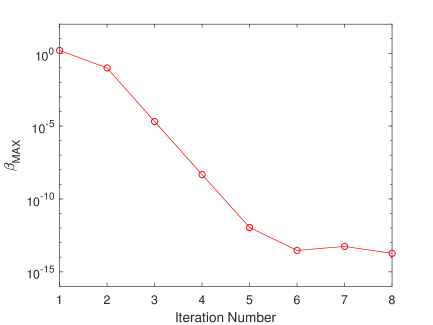
Figure 1: Curve of $\beta_{\rm MAX}$ versus the iteration number.

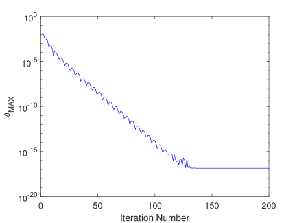
Figure 2: Curve of $\delta_{\rm MAX}$ versus the iteration number.

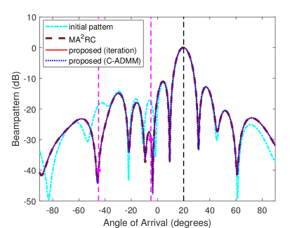
((a)) The first step

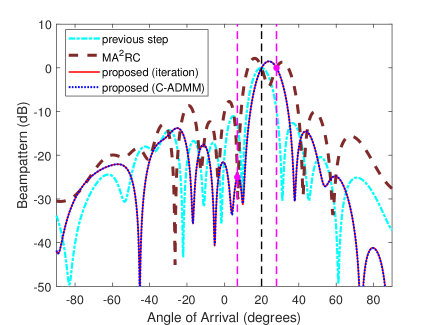
((b)) The second step

Figure 3: Illustration of multi-point OPARC algorithm.

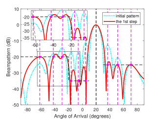
((a)) Synthesized pattern at the 1st step

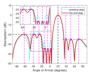
((b)) Synthesized pattern at the 2nd step

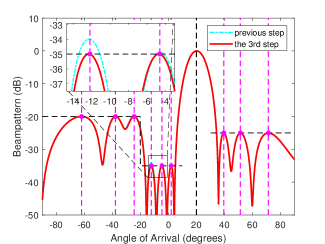
((c)) Synthesized pattern at the 3rd step

Figure 4: Resultant patterns at different steps when carrying out a nonuniform sidelobe synthesis for a nonuniform linear array.

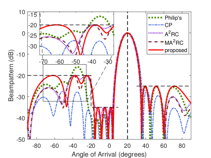
Figure 5: Resultant pattern comparison.

More specifically, we set $\theta_{1,1}=-45^{\circ}$, ${\rho}_{1,1}=-40{\rm dB}$, $\theta_{1,2}=-5^{\circ}$ and ${\rho}_{1,2}=-30{\rm dB}$ for the first step of the response control. Note that the same settings have been adopted in Section V.A in Part I [1], where the single-point response control is realized in sequence. In this part, we first conduct multi-point OPARC algorithm by using the iterative method described in Algorithm 1. In the first iteration, the OPARC algorithm in [1] is applied to control the responses of $\theta_{1,m}$ to their desired levels $\rho_{1,m}$, $m=1,2$, one-by-one on $m$. We have ${\beta}_{1,1,\star}=1.5683$, ${\beta}_{1,2,\star}=0.2504$, which is the same as the results obtained in Section V.A in Part I [1]. Then, we continue our multi-point OPARC algorithm by conducting the above iteration procedure for a number of times. The curve of $\beta_{\rm MAX}$ versus the iteration number is depicted in Fig. 1. Note that the parameter $\beta_{\rm MAX}$ measures the maximal magnitudes of INRs of the newly assigned virtual interferences in the current iteration, as shown in the 8th line of Algorithm 1. From Fig. 1, one can see that $\beta_{\rm MAX}$ decreases with iteration. Moreover, observation shows that it only requires five iterations to converge, i.e., ${\beta}_{\rm MAX}\leq{\beta}_{\epsilon}$, and the result is $\bar{\beta}_{1,1,\star}=1.4700$ and $\bar{\beta}_{1,2,\star}=0.2506$, which is, respectively, close to ${\beta}_{1,1,\star}$ and ${\beta}_{1,2,\star}$. Now we test the performance of the C-ADMM approach. The obtained $\delta_{\rm MAX}$ in (32) reduces with the iteration, i.e., the procedure described in (II-D2)-(31), as shown in Fig. 2, and ${\delta}_{\rm MAX}\leq{\delta}$ is met after about 130 iterations. We obtain ${\bf h}_{1,\star}=[-0.1458-j0.0203,-0.0687-j0.0397]^{\mathop{\rm T}}$. Not surprisingly, it can be checked that the results of the above two approaches correspond to the same weight vector. Hence, the same beampatterns are synthesized for these two approaches as shown in Fig. 3(a), from which one can see that the responses of the two adjusted angles have been precisely controlled to their desired values. Interestingly, when testing the ${\textrm{M}}{\textrm{A}}^{2}{\textrm{RC}}$, the resulting pattern is completely the same as that of the multi-point OPARC algorithm. We believe that this occurs not accidentally but with a reason that is, unfortunately, not clear yet.

TABLE I: Obtained Parameter Comparison

	${\textrm{M}}{\textrm{A}}^{2}{\textrm{RC}}$	Multi-point OPARC
$D_{1}({\rm dB})$	$21.3110$	$5.7620$
$D_{2}({\rm dB})$	$13.5149$	$10.0816$
$J$	$0.3132$	$0.1909$
$G_{1}({\rm dB})$	$10.0078$	$10.0078$
$G_{2}({\rm dB})$	$9.9192$	$11.2550$

In the second step of the response control, we take $\theta_{2,1}=7^{\circ}$, ${\rho}_{2,1}=-25{\rm dB}$, $\theta_{2,2}=28^{\circ}$ and ${\rho}_{2,2}=0{\rm dB}$. When conducting the multi-point OPARC algorithm, we obtain $\bar{\beta}_{2,1,\star}=0.2555$ and $\bar{\beta}_{2,2,\star}=-0.0804$ for the iterative approach, and find ${\bf h}_{2,\star}=[-0.1803-j0.0653,-0.5434-j0.9252]^{\mathop{\rm T}}$ after implementing the C-ADMM method. Again, the above two sets of results correspond to the same beampattern as shown in Fig. 3(b), where the resulting pattern of ${\textrm{M}}{\textrm{A}}^{2}{\textrm{RC}}$ is also displayed. From Fig. 3(b), one can see that all the adjusted angles have been accurately controlled as expected, for the three approaches. However, the mainlobe of the ultimate pattern of ${\textrm{M}}{\textrm{A}}^{2}{\textrm{RC}}$ is distorted and a high sidelobe level is resulted. For comparison purpose, we have listed several parameter measurements in Table I, from which one can see that the ${\textrm{M}}{\textrm{A}}^{2}{\textrm{RC}}$ method brings large values on both $D_{k}$ ($k=1,2$) and $J$, and results a less array gain compared to the proposed multi-point OPARC algorithm.

IV-B Array Pattern Synthesis Using Multi-point OPARC

Starting from this subsection, the applications of multi-point OPARC are simulated and the iterative approach in Section II. C is adopted to illustrate the results. In this subsection, we focus upon the application of multi-point OPARC to array pattern synthesis and give two representative examples for demonstration.

IV-B1 Nonuniform Sidelobe Synthesis

In the first example, the desired pattern has nonuniform sidelobes. Fig. 4 shows the synthesized patterns of the proposed algorithm at different steps. Clearly, in each synthesis step, all the sidelobe peaks, i.e., ${\Omega}_{k}$ in (42), are first determined from the previously synthesized pattern. Notice that the response level of a selected sidelobe peak can be either higher or lower (see Fig. 4(a) for reference) than its desired level. It has been shown in Fig. 4 that it only requires 3 steps, i.e., $k=3$, to synthesize a satisfactory beampattern.

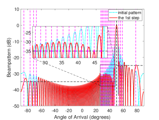
((a)) Synthesized pattern at the 1st step

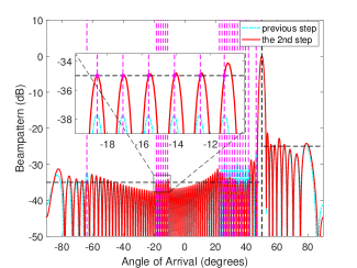
((b)) Synthesized pattern at the 2nd step

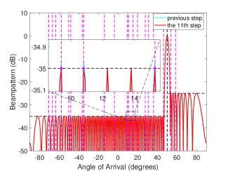
((c)) Synthesized pattern at the 11th step

Figure 6: Resultant patterns at different steps when carrying out a nonuniform sidelobe synthesis for a large uniform linear array.

For comparison, the resulting patterns of the proposed algorithm, Philip’s method in [11], convex programming (CP) method in [8], ${\textrm{A}}^{2}\textrm{RC}$ method (after carrying out 30 steps) in [3] and ${\textrm{M}}{\textrm{A}}^{2}\textrm{RC}$ method (after carrying out 3 steps) in [2] are displayed in Fig. 5. As expected, we can see that the pattern envelopes of Philip ’s method and CP method are not aligned with the desired level, since they cannot control the beampattern precisely according to the required specifications. Although ${\textrm{A}}^{2}\textrm{RC}$ and ${\textrm{M}}{\textrm{A}}^{2}\textrm{RC}$ have the ability to precisely control the given array responses, the obtained sidelobe peaks are not aligned with the desired ones either, since only the sidelobe peaks higher than the desired levels are selected and adjusted in these two approaches.

TABLE II: Execution Time Comparison When Conducting a Large-array Pattern Synthesis

	Philip’s	CP	$~{}{\textrm{A}}^{2}\textrm{RC}~{}$	${\textrm{M}}{\textrm{A}}^{2}\textrm{RC}$	proposed
$T(\rm sec)$	2.22	12.36	3.55	2.55	0.05

IV-B2 Large Array Consideration

In this example, pattern synthesis for a large linearly half-wavelength-spaced array with $N=80$ isotropic elements is considered. The desired pattern steers at $\theta_{0}=50^{\circ}$ with nonuniform sidelobes. More specifically, the upper level is $-35{\rm dB}$ in the sidelobe region $[-90^{\circ},50^{\circ})$ and $-25{\rm dB}$ in the rest of the sidelobe region.

Fig. 6 demonstrates several intermediate results of the proposed algorithm. In every step, we select $C_{k}=20$ sidelobe peak angles (see Eqn. (43) and (44) for details) and then adjust their responses to the desired levels by using multi-point OPARC algorithm. Simulation result shows that it only requires $11$ steps, i.e., $k=11$, to synthesize a qualified pattern, see the ultimate pattern in Fig. 6(c) for reference. The execution times of various methods are provided in Table II, where the superiority of the proposed algorithm can be clearly observed.

IV-C Multi-constraint Adaptive Beamforming Using Multi-point OPARC

In this subsection, the multi-constraint adaptive beamforming is realized by using the multi-point OPARC algorithm. For simplicity, a perfect knowledge of the data covariance matrix is assumed.

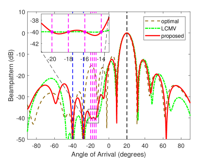
((a)) The first case

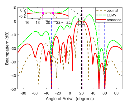
((b)) The second case

Figure 7: Result comparison of multi-constraint adaptive beamforming.

IV-C1 Sidelobe Constraint

In the first case, four sidelobe constraints are required. More specifically, the response levels of $-20^{\circ}$, $-18^{\circ}$, $-16^{\circ}$ and $-14^{\circ}$ are expected to be all $-40{\rm dB}$. Two interferences are impinged from $-40^{\circ}$ and $-28^{\circ}$ with INRs $30{\rm dB}$ and $25{\rm dB}$, respectively.

Fig. 7(a) displays the results of the optimal beamformer with no sidelobe constraint, the LCMV method [13] and the proposed one. Clearly, both the LCMV beamformer and the proposed algorithm are able to shape deep nulls at the directions of interferences (see the blue line). Meanwhile, the given sidelobe constraints are well satisfied for both. When considering the output SINR, we have ${\rm SINR}=19.5601{\rm dB}$ for the LCMV method and ${\rm SINR}=19.6906{\rm dB}$ for the proposed one. We can see that the proposed beamformer brings an improvement on the output SINR compared to the LCMV beamformer.

IV-C2 Mainlobe Constraint

In the second case, two constraints are imposed in the mainlobe region. The constraint angles are $19^{\circ}$ and $21^{\circ}$, and both of the desired levels are $0{\rm dB}$. There are three interferences coming from $-32^{\circ}$, $50^{\circ}$ and $60^{\circ}$ with an identical INR $30{\rm dB}$.

Fig. 7(b) depicts the resultant patterns. One can see that the obtained pattern of the LCMV method is severely distorted, although the two prescribed constraints are satisfied and the three interferences are rejected. The corresponding output SINR is $11.1767{\rm dB}$. Observing the resulting pattern of the proposed algorithm, the two-point constraint is well satisfied and a flat-top mainlobe is shaped with no distortion occurred. The corresponding output SINR is $17.1260{\rm dB}$, which is much higher than that of the LCMV method.

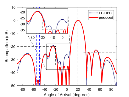
((a)) The first case

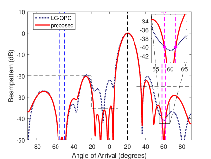
((b)) The second case

Figure 8: Result comparison of quiescent pattern control.

IV-D Quiescent Pattern Control Using Multi-point OPARC

In this subsection, we test the performance of the multi-point OPARC based quiescent pattern control algorithm. The desired quiescent pattern has a nonuniform sidelobe level as depicted with black dash lines in Fig. 5.

In our proposed algorithm, quiescent pattern synthesis and quiescent pattern control are jointly designed by the multi-point OPARC algorithm. We have detailed the off-line synthesis procedure in Section IV.B and illustrated the obtained quiescent pattern by red line in Fig. 5. Suppose that two interferences come from $-55^{\circ}$ and $-49^{\circ}$ with INRs $30{\rm dB}$. The obtained adaptive response pattern is shown in Fig. 8(a), where we can observe that two nulls are formed at the directions of the real interferences, and the resultant sidelobe is close to the quiescent one. The obtained output SINR is $19.2984{\rm dB}$ for the proposed algorithm.

For comparison purpose, the classical linearly-constraint based quiescent pattern control approach (denoted as LC-QPC method for briefness) in [19] is also demonstrated, by using the same synthesized quiescent pattern in Fig. 5. The resulting pattern of LC-QPC is displayed in Fig. 8(a), where we find that an obvious perturbation is caused in the sector $[-15^{\circ},0^{\circ}]$ and the overall shape can not be well maintained compared to the desired one. The obtained output SINR is $19.2161{\rm dB}$, which is lower than that of the proposed algorithm.

Now we take extra fixed constraints into consideration by restricting the response levels at directions $58^{\circ}$ and $62^{\circ}$ to be all $-40{\rm dB}$. The results of the proposed algorithm and the LC-QPC method are presented in Fig. 8(b), where we observe that both of these two methods are able to reject the undesirable interferences with the prescribed constraints being satisfied. The same as before, the proposed algorithm maintains a more desirable shape than that of the LC-QPC method. When taking the output SINR into account, the corresponding values are, respectively, $19.2382{\rm dB}$ (for the proposed algorithm) and $19.0967{\rm dB}$ (for the LC-QPC method). The advantage of the proposed algorithm is verified again.

V Conclusions

In this paper, the optimal and precise array response control (OPARC) algorithm proposed in Part I [1] has been extended from a single point per step to a multi-points per step. Two computationally attractive multi-point OPARC algorithms have been proposed, by which the responses of multiple angles can be adjusted. In addition, several applications of the multi-point OPARC algorithm to array signal processing have been presented, and an innovate concept of normalized covariance matrix loading (NCL) has been developed. Simulation results have been provided to validate the effectiveness and superiority of the proposed algorithms under different situations.

References

- [1] X. Zhang, Z. He, X.-G. Xia, B. Liao, X. Zhang, and Y. Yang, “OPARC: optimal and precise array response control algorithm – Part I: Fundamentals,” preprint, Dec. 2017.
- [2] X. Zhang, Z. He, B. Liao, X. Zhang, and W. Peng, “Pattern synthesis with multipoint accurate array response control,” IEEE Trans. Antennas Propag., vol. 65, pp. 4075-4088, 2017.
- [3] X. Zhang, Z. He, B. Liao, X. Zhang, Z. Cheng, and Y. Lu, “: an accurate array response control algorithm for pattern synthesis,” IEEE Trans. Signal Process., vol. 65, pp. 1810-1824, 2017.
- [4] K. Huang and N. D. Sidiropoulos, “Consensus-ADMM for general quadratically constrained quadratic programming,” IEEE Trans. Signal Process., vol. 64, pp. 5297-5310, 2016.
- [5] K. Chen, X. Yun, Z. He, and C. Han, “Synthesis of sparse planar arrays using modified real genetic algorithm,” IEEE Trans. Antennas Propag., vol. 55, pp. 1067-1073, 2007.
- [6] V. Murino, A. Trucco, and C. S. Regazzoni, “Synthesis of unequally spaced arrays by simulated annealing,” IEEE Trans. Signal Process., vol. 44, pp. 119-122, 1996.
- [7] D. W. Boeringer and D. H. Werner, “Particle swarm optimization versus genetic algorithms for phased array synthesis,” IEEE Trans. Antennas Propag., vol. 52, pp. 771-779, 2004.
- [8] H. Lebret and S. Boyd, “Antenna array pattern synthesis via convex optimization,” IEEE Trans. Signal Process., vol. 45, pp. 526-532, 1997.
- [9] W. Fan, V. Balakrishnan, P. Y. Zhou, J. J. Chen, R. Yang, and C. Frank, “Optimal array pattern synthesis using semidefinite programming,” IEEE Trans. Signal Process., vol. 51, pp. 1172-1183, 2003.
- [10] B. Fuchs, “Application of convex relaxation to array synthesis problems,” IEEE Trans. Antennas Propag., vol. 62, pp. 634–640, 2014.
- [11] P. Y. Zhou and M. A. Ingram, “Pattern synthesis for arbitrary arrays using an adaptive array method,” IEEE Trans. Antennas Propag., vol. 47, pp. 862-869, 1999.
- [12] K. Yang, Z. Zhao, and Q. H. Liu, “Fast pencil beam pattern synthesis of large unequally spaced antenna arrays,” IEEE Trans. Antennas Propag., vol. 61, pp. 627-634, 2013.
- [13] O. L. Frost, III, “An algorithm for linearly constrained adaptive array processing,” Proc. IEEE, vol. 60, pp. 926-935, 1972.
- [14] J. Xu, G. Liao, S. Zhu, and L. Huang, “Response vector constrained robust lcmv beamforming based on semidefinite programming,” IEEE Trans. Signal Process., vol. 63, pp. 5720-5732, 2015.
- [15] C. Y. Chen and P. P. Vaidyanathan, “Quadratically constrained beamforming robust against direction-of-arrival mismatch,” IEEE Trans. Signal Process., vol. 55, pp. 4139-4150, 2007.
- [16] H. Cox, R. Zeskind, and M. Owen, “Robust adaptive beamforming,” IEEE Trans. Acoust., Speech, Signal Process., vol. 35, pp. 1365-1376, 1987.
- [17] B. D. Carlson, “Covariance matrix estimation errors and diagonal loading in adaptive arrays,” IEEE Trans. Aerosp. Electron. Syst., vol. 24, pp. 397-401, 1988.
- [18] J. Li, P. Stoica, and Z. Wang, “On robust Capon beamforming and diagonal loading,” IEEE Trans. Signal Process., vol. 51, pp. 1702-1715, 2003.
- [19] L. Griffiths and K. Buckley, “Quiescent pattern control in linearly constrained adaptive arrays,” IEEE Trans. Acoust., Speech, Signal Process., vol. 35, pp. 917-926, 1987.
- [20] B. D. V. Veen, “Optimization of quiescent response in partially adaptive beamformers,” IEEE Trans. Acoust., Speech, Signal Process., vol. 38, pp. 471-477, 1990.
- [21] C. Y. Tseng and L. J. Griffiths, “A unified approach to the design of linear constraints in minimum variance adaptive beamformers,” IEEE Trans. Antennas Propag., vol. 40, pp. 1533-1542, 1992.
- [22] H. K. Van Trees, Optimum Array Processing. New York: Wiley, 2002.
- [23] G. H. Golub and C. F. V. Loan, Matrix Computations. Baltimore, MD: The Johns Hopkins Univ. Press, 1996.
- [24] S. Boyd, N. Parikh, E. Chu, B. Peleato, and J. Ecksein, “Distributed optimization and statistical learning via the alternating direction method of multipliers,” Found. Trends Mach. Learn., vol. 3, no. 1, pp. 1 C122, 2011.
- [25] J. Park and S. Boyd, “General heuristics for nonconvex quadratically constrained quadratic programming,” available online: http://stanford.edu/~boyd/papers/pdf/qcqp.pdf.
- [26] A. Liu, G. Liao, C. Zeng, Z. Yang, and Q. Xu, “An eigenstructure method for estimating DOA and sensor gain-phase errors,” IEEE Trans. Signal Process., vol. 59, pp. 5944-5956, 2011.