GRAY RADIATION HYDRODYNAMICS WITH THE FLASH CODE FOR ASTROPHYSICAL APPLICATIONS

Abstract

We present the newly–incorporated gray radiation hydrodynamics capabilities of the FLASH code based on a radiation flux–limiter aware hydrodynamics numerical implementation designed specifically for applications in astrophysical problems. The implemented numerical methods consist of changes in the unsplit hydrodynamics solver and adjustments in the flux–limited radiation diffusion unit. Our approach can handle problems in both the strong and weak radiation–matter coupling limits as well as transitions between the two regimes. Appropriate extensions in the “Helmholtz” equation of state are implemented to treat two–temperature astrophysical plasmas involving the interaction between radiation and matter and the addition of a new opacity unit based on the OPAL opacity database, commonly used for astrophysical fluids. A set of radiation–hydrodynamics test problems is presented aiming to showcase the new capabilities of FLASH and to provide direct comparison to other similar software instruments available in the literature. To illustrate the capacity of FLASH to simulate phenomena occurring in stellar explosions, such as shock break–out, radiative precursors and supernova ejecta heating due to the decays of radioactive ⁵⁶Ni and ⁵⁶Co, we also present 1D supernova simulations and compare the computed lightcurves to those of the SNEC code. The latest public release of FLASH with these enhanced capabilities is available for download and use by the broader astrophysics community.

1. INTRODUCTION

The analysis and interpretation of electromagnetic signals is by far the main source of information used to study astrophysical phenomena. In this regard, the importance to understand the interaction between radiation and matter and the physics of radiation transfer is pivotal to gaining comprehensive insights about the underlying physical mechanisms.

Due to the complexity of radiation transport physics combined with the dynamics of strongly ionized plasmas that can, in some cases, possess supersonic motions, most astrophysical problems require numerical simulations for proper examination. A number of codes have been designed that use a multitude of numerical techniques to calculate model light–curves (LCs), spectra, polarization spectra and radiation–driven hydrodynamic flows for direct comparison with observations.

To model the diffusion of light through expanding matter for the purposes of computing supernova (SN) LCs, there are codes that use multi–group time–dependent non–equilibrium radiative transfer (for example, the STELLA code of Blinnikov et al. 1998, that incorporates a radiation intensity moments scheme). Frequently, there are simpler numerical approaches used that are based on the flux–limited diffusion approximation (FLD; Minerbo 1978; Levermore & Pomraning 1981; Clarke 1996). Examples of such codes that are often used to compute SN LCs include the SPECTRUM code (Frey et al., 2013), and the publicly available SNEC code (Morozova et al., 2015).

The radiation diffusion approximation is useful in providing us with the general emission properties and model LCs for SNe, but a more rigorous approach requires accurate, time–dependent spectroscopic modeling. Spectroscopic modeling can be computationally expensive, especially in 2D and 3D geometries, because it involves making use of large databases of line opacities in order to calculate emission and absorption line profiles taking into account many factors including material composition, density, temperature and velocity. Currently, many spectral modeling codes are used in a post–processing manner; pure or radiation hydrodynamical “snapshot” profiles are extracted from other codes and then used as inputs to the (usually) Lagrangian grids of radiation transport codes yielding model spectra. Some spectral sythesis codes employ Monte Carlo techniques to model radiation transfer and are optimized for both the local (LTE) and non–local thermal equillibrium (nLTE) limits. Examples of some of the most popular codes used include CMFGEN (Hillier & Dessart, 2012), SEDONA (Kasen et al., 2006), PHOENIX (Hauschildt & Baron, 1999; Hauschildt, 1992; Hauschildt & Baron, 2004; van Rossum, 2012), SuperNu (Wollaeger et al., 2013) and the open–source CLOUDY (Ferland et al., 1998) and TARDIS (Kerzendorf & Sim, 2014) codes. Some of these codes have been routinely used to study emission from expanding SN photopsheres and have been succesfully compared to a lot of observations.

Radiation hydrodynamics (Mihalas & Mihalas, 1984; Castor, 2007) is necessary to study the propagation and properties of radiative shocks, supernova remnant (SNR) emission, supernova (SN) shock breakout, and radiation–driven mass loss from massive stars near the Eddington limit, to name just a few phenomena. The applicability of the concepts of radiation hydrodynamics in sensitive fields like nuclear weapons simulations and high-energy-density laser experiments has led to the development of codes with such capabilities in government laboratories like the Los Alamos National Laboratory and the Lawrence Berkeley National Laboratory, several of which are inaccessible for use by most academic researchers.

However, the advent of open–source or publicly available computational astrophysics codes like MESA (Paxton et al., 2011, 2013, 2015) for stellar evolution, FLASH for hydrodynamics, SNEC for equilibrium–diffusion radiation transport and TARDIS for spectral synthesis has energized the field of computational astrophysics by making these essential modeling tools available for use to everyone in the community, from graduate students to senior researchers, and thus fostering collaboration and transparency. Other notable examples of open–access radiation hydrodynamics codes include ZEUS (Stone et al., 1992), HERACLES (González et al., 2007), RAGE (Gittings et al., 2008), CRASH (van der Holst et al., 2011), RAMSES (Commerçon et al., 2011), ENZO (Wise & Abel, 2011) and CASTRO (Zhang et al., 2011, 2013).

The FLASH (Fryxell et al., 2000; Dubey et al., 2012) adaptive–mesh refinement magnetohydrodynamics (MHD) code is very popular amongst the numerical astrophysics community – especially in the supernova field – with applications ranging from studies of Type Ia SNe (Calder et al., 2004; Townsley et al., 2007), core–collapse SNe (Couch, 2013a; Couch & O’Connor, 2013), pair–instability SNe (Chatzopoulos et al., 2013) and pre–SN convection (Couch, 2013b; Chatzopoulos et al., 2014). In addition, FLASH is amongst the best documented software instruments online with continuous development and support provided through an active mailing list. Nonetheless, the important component of a two–temperature (2T) radiation hydrodynamics treatment was missing from the code thus restricting the capacity to simulate a variety of interesting problems and obtain predictions, such as numerical SN LCs, that can be directly compared with observations. For this reason, and to contribute to the open computational astrophysics community, we introduce our recently implemented gray FLD radiation hydrodynamics scheme of the FLASH code optimized for astrophysical applications and designed with emphasis on simulating physical processes that are important within the supernova field: the Radiation Flux–Limiter Aware Hydrodynamics scheme (RadFLAH). Our approach and numerical methods are tested in a variety of contexts and physical domains and benchmarked against analytical predictions and published results of other codes. The latest release of FLASH (version 4.5) includes RadFLAH and is available for download. Some documentation is also available within the FLASH user’s guide.

The paper is organized as follows. In § 2 we present the set of radiation–hydrodynamics equations in the gray FLD limit that we are numerically solving. In § 3 we discuss in more detail the numerical techniques implemented in the FLASH framework to solve that system of equations, namely our radiation flux–limiter aware hydrodynamics (RadFLAH) method. A set of test problems illustrating the new capabilities of the code is presented in § 4, and a special application for 1D spherical supernova explosions is discussed in § 5. Finally, in § 6 we discuss our conclusions and the importance of having an open–source tool to study radiation–hydrodynamics in astrophysics.

2. RADIATION HYDRODYNAMICS IN THE FLUX-LIMITED DIFFUSION LIMIT

Our implementation is based on gray FLD methods that are suitable in avoiding the main issue of faster–than–light signal propagation when the diffusion equation is applied in the optically–thin regime. Although FLD is one of the most commonly–used and well–established methods (Minerbo, 1978; Levermore & Pomraning, 1981; Clarke, 1996) it has known limitations such as the treatment of radiation flows in the free–streaming limit. In this regime various implementations of FLD rely on different forms of flux–limiters that often result in notably different results when simulating standard radiation hydrodynamics test problems (see, for example 4.4).

As a starting point, we take the equations for mixed-frame FLD radiation hydrodynamics developed in Krumholz et al. (2007). Adopting notation for our purposes, we write

$$\frac{\partial\rho}{\partial t}+\nabla\cdot(\rho{\mathitbf{v}})=0\,,\,$$ (1)

$$\frac{\partial(\rho{\mathitbf{v}})}{\partial t}+\nabla\cdot(\rho{\mathitbf{v}}\mathop{\otimes}\mathop{{\mathitbf{v}}})+\nabla p+\lambda\nabla E_{\mathrm{r}}=0\,,\,$$ (2)

$$\frac{\partial E_{\mathrm{m}}}{\partial t}+\nabla\cdot\left[(E_{\mathrm{m}}+p){\mathitbf{v}}\right]-\lambda\left(2\frac{\kappa_{\rm P}}{\kappa_{\rm R}}-1\right){\mathitbf{v}}\cdot\nabla E_{\mathrm{r}}$$

$$=-\kappa_{\rm P}(4\pi B-cE_{\mathrm{r}})\,,\,$$ (3)

$$\frac{\partial E_{\mathrm{r}}}{\partial t}+\nabla\cdot\left[(1+\lambda^{\prime})E_{\mathrm{r}}{\mathitbf{v}}\right]+\lambda\left(2\frac{\kappa_{\rm P}}{\kappa_{\rm R}}-1\right){\mathitbf{v}}\cdot\nabla E_{\mathrm{r}}$$

$$=\nabla\cdot\left(\frac{c\lambda}{\kappa_{\rm R}}\nabla E_{\mathrm{r}}\right)+\kappa_{\rm P}(4\pi B-cE_{\mathrm{r}})\,.\,$$ (4)

Here $\kappa_{\rm P}$ and $\kappa_{\rm R}$ are the Planck (absorption) and Rosseland (transport) coefficients respectively and $B$ is the Planck function. Also, $E_{\mathrm{m}}$ is the matter energy density, defined by the relation $E_{\mathrm{m}}=\rho e_{\mathrm{m}}+\rho\frac{{\mathitbf{v}}^{2}}{2}$ (where $e_{\mathrm{m}}$ is specific internal matter energy), and $E_{\mathrm{r}}$ is the radiation energy density. We make the approximation that the flux limiter $\lambda$ depends on radiation energy density $E_{\mathrm{r}}$ in the lab frame (rather than a comoving density $E_{\mathrm{r}}^{(0)}$). Thus $\lambda=\lambda(R)$ depends on the quantity $R=\frac{\left|\nabla E_{\mathrm{r}}\right|}{\kappa_{R}E_{\mathrm{r}}}$, and we have further introduced the abbreviation $\lambda^{\prime}=\frac{1-f}{2}$, where $f=\lambda+\lambda^{2}R^{2}$ is the Eddington factor. Note that both $\lambda$ and $\lambda^{\prime}$ have similar asympotic behavior for both the diffusion limit ($\lambda,\lambda^{\prime}\rightarrow 1/3$ for $R\rightarrow 0$) and the free–streaming limit ($\lambda,\lambda^{\prime}\rightarrow 0$ for $R\rightarrow\infty$); moreover, as pointed out in Zhang et al. (2011); their difference remains small for all $0<R<\infty$.

Our implementation uses operator splitting to separate this system of equations into an “enhanced hydro” subsystem and a “radiation transfer” subsystem. The latter describes the effect of the terms written on the right–hand side in Equations 1– 4 above, and is equivalent to

$$\rho\frac{\partial e_{\mathrm{m}}}{\partial t} = -\kappa_{\rm P}(4\pi B-cE_{\mathrm{r}})\,,\,$$ (5)

$$\frac{\partial E_{\mathrm{r}}}{\partial t} = \nabla\cdot\left(\frac{c\lambda}{\kappa_{\rm R}}\nabla E_{\mathrm{r}}\right)+\kappa_{\rm P}(4\pi B-cE_{\mathrm{r}})\,.\,$$ (6)

The former consists of Equations. 1–4 with right hand sides set to 0; we call our approach to solving this system Radiation Flux–Limiter Aware Hydrodynamics (RadFLAH). By adding the last two of those modified equations,

$$\frac{\partial E_{\mathrm{m}}}{\partial t}+\nabla\cdot[(E_{\mathrm{m}}+p){\mathitbf{v}}]-\lambda(2\frac{\kappa_{\rm P}}{\kappa_{\rm R}}-1){\mathitbf{v}}\cdot\nabla E_{\mathrm{r}}=0\,,\,$$ (7)

$$\frac{\partial E_{\mathrm{r}}}{\partial t}+\nabla\cdot[(1+\lambda^{\prime})E_{\mathrm{r}}{\mathitbf{v}}]+\lambda(2\frac{\kappa_{\rm P}}{\kappa_{\rm R}}-1){\mathitbf{v}}\cdot\nabla E_{\mathrm{r}}=0\,,\,$$ (8)

we get the following equation:

$$\frac{\partial}{\partial t}(E_{\mathrm{m}}+E_{\mathrm{r}})+\nabla\cdot\left[(E_{\mathrm{m}}+p+(1+\lambda^{\prime})E_{\mathrm{r}}){\mathitbf{v}}\right]=0\,.\,$$ (9)

This can also be written

$$\frac{\partial E_{\mathrm{tot}}}{\partial t}+\nabla\cdot\left[(E_{\mathrm{tot}}+P_{\mathrm{tot}}+p_{\Lambda}){\mathitbf{v}}\right]=0\,,\,$$ (10)

with $E_{\mathrm{tot}}=E_{\mathrm{m}}+E_{\mathrm{r}}$ and $P_{\mathrm{tot}}=p+\lambda E_{\mathrm{r}}$ and a small correction term $p_{\Lambda}=(\lambda^{\prime}-\lambda)E_{\mathrm{r}}$.

For further reference, we also write an equivalent equation for matter internal specific energy:

$$\frac{\partial(\rho e_{\mathrm{m}})}{\partial t}+\nabla\cdot(\rho e_{\mathrm{m}}{\mathitbf{v}})+p\nabla\cdot{\mathitbf{v}}-2\lambda\frac{\kappa_{\rm P}}{\kappa_{\rm R}}{\mathitbf{v}}\cdot\nabla E_{\mathrm{r}}=0\,.\,$$

3. NUMERICAL METHODS

The goal of the RadFLAH code is to solve the (overdetermined) system of five equations (1),(2),(7),(8),(10). This could be done by directly implementing a hyperbolic solver for a system consisting of equations (1), (2), and any two of (7), (8), and (10). We will instead first solve the system of three equations (1),(2),(10) numerically for a time step, thus computing new values of $\rho$, ${\mathitbf{v}}$, and total energy $E_{\mathrm{tot}}$, and then use this solution together with (2) and (8) to distribute the total energy change (computed directly from (10)) to the energies $E_{\mathrm{m}}$ and $E_{\mathrm{r}}$.

FLASH already provides a variety of directionally unsplit methods for solving the system of Euler equations of hydrodynamics (HD), as well as the equations of magnetohydrodynamics (MHD). These are based on the Godunov approach and feature a variety of Riemann solvers, orders of reconstruction, slope limiters, and related features. The HD and MHD solvers can work with a variety of equation of state (EOS) models by using a formulation derived from Colella & Glaz (1985). In addition to advancing the core variables of HD or MHD, FLASH can also advect arbitrary additional variables $X$ (“mass scalars”), equivalent to solving additional equations

$$\frac{\partial(\rho X)}{\partial t}+\nabla\cdot(\rho X{\mathitbf{v}})=0\,.\,$$ (12)

Our approach has been to reuse as much of this existing code as possible. Here we outline this approach; some more implementation details can be found in the appendix.

First, we write the fluid state in conservative form as

$${\mathitbf{U}}=\begin{pmatrix}\rho\cr\rho{\mathitbf{v}}\cr E_{\mathrm{tot}}\cr\rho e_{\mathrm{m}}\cr E_{\mathrm{r}}\cr X_{1}\rho\cr\vdots\cr X_{n}\rho\end{pmatrix}$$ (13)

and our evolution equations as

$$\frac{\partial}{\partial t}{\mathitbf{U}}=f^{[1]}+f^{[2]}+f^{[3]}+f^{[4]}\\ =f_{hyperbolic}+f_{fixup}+f_{Lorentz}+f_{transp}.$$ (14)

Here

$$f^{[1]}=f_{hyperbolic}=\begin{pmatrix}-\nabla\cdot(\rho{\mathitbf{v}})\cr-\nabla\cdot(\rho{\mathitbf{v}}{\mathitbf{v}})-\nabla p-\lambda\nabla E_{\mathrm{r}}\cr-\nabla\cdot\left[(E_{\mathrm{tot}}+P_{\mathrm{tot}}+p_{\Lambda}){\mathitbf{v}}\right]\cr-\nabla\cdot\left(\rho e_{\mathrm{m}}{\mathitbf{v}}\right)\cr-\nabla\cdot\left[(1+\lambda^{\prime})E_{\mathrm{r}}{\mathitbf{v}}\right]\cr-\nabla\cdot(\rho X_{1}{\mathitbf{v}})\cr\vdots\cr-\nabla\cdot(\rho X_{n}{\mathitbf{v}})\cr\end{pmatrix},$$ (15)

$$f^{[2]}=f_{fixup}=\begin{pmatrix}0\cr\mathbf{0}\cr 0\cr-p\,\nabla\cdot{\mathitbf{v}}\cr\lambda{\mathitbf{v}}\cdot\nabla E_{\mathrm{r}}\cr 0\cr\vdots\cr 0\end{pmatrix},$$ (16)

$$f^{[3]}=f_{Lorentz}=\begin{pmatrix}0\cr\mathbf{0}\cr 0\cr 2\lambda\frac{\kappa_{\rm P}}{\kappa_{\rm R}}{\mathitbf{v}}\cdot\nabla E_{\mathrm{r}}\cr-2\lambda\frac{\kappa_{\rm P}}{\kappa_{\rm R}}{\mathitbf{v}}\cdot\nabla E_{\mathrm{r}}\cr 0\cr\vdots\cr 0\end{pmatrix},$$ (17)

and

$$f^{[4]}=f_{transp}=\begin{pmatrix}0\cr\mathbf{0}\cr\nabla\cdot\left(\frac{c\lambda}{\kappa_{\rm R}}\nabla E_{\mathrm{r}}\right)\cr-\kappa_{\rm P}(4\pi B-cE_{\mathrm{r}})\cr\nabla\cdot\left(\frac{c\lambda}{\kappa_{\rm R}}\nabla E_{\mathrm{r}}\right)+\kappa_{\rm P}(4\pi B-cE_{\mathrm{r}})\cr 0\cr\vdots\cr 0\end{pmatrix}.$$ (18)

The numerical advance of the solution from state $U^{(n)}$ to $U^{(n+1)}$ by a time step $\Delta t$ can then be performed in several successive phases $\rm p\in\{1,2,3,4\}$:

$$U^{(n)[1]}=U^{(n)}+\Delta t\\ f^{[1]},$$ (19)

$$U^{(n)[p]}=U^{(n)[\rm p-1]}+\Delta t\\ f^{[\rm p]},\\ \\ \ \rm p=2,...,4,$$ (20)

$$U^{(n+1)}=U^{(n)[4]},$$ (21)

where the term $f^{[1]}$ corresponds to divergence of fluxes while the other terms $f^{[2,3,4]}$ are not. We now briefly describe the meaning of each term:

• $U^{(n)[1]}$: This term corresponds to the conservative form of our modified hydrodynamics implementation that is described in detail below (Section 3.1).

• $U^{(n)[2]}$: Non–hyperbolic additional modified–hydro term. In practice, these steps are computed within the regular FLASH unsplit hydrodynamics unit, as an add–on action after the main update. Note, that this term only modifies the component energies, not conserved totals.

• $U^{(n)[3]}$: An additional coupling term of relativistic nature. This term is also computed within the hydrodynamics unit, as an add–on action after the main update; but could also be separated out of hydro and be done as part of phase 4 (we plan to include this capability in a future version). This term only modifies the individual (radiation, matter) component energies, not the conserved totals.

• $U^{(n)[4]}$: The radiation transport component. This is completely separate from the hydrodynamics component and is included here to facilitate term–by–term comparison with other papers.

We must add that the implementation of $U^{(n)[4]}$ is not the central subject of this paper, since we are using two pre–existing methods of previous versions of FLASH. What is new is that we are using them in the context of the 2T RadFLAH implementation. These original methods include a flux limiter and allow us to expand to alternative flux limiter implementations. As such, we are using the same flux–limiter formulation for additional purposes within the modified hydrodynamics implementation.

3.1. Modified hydrodynamics.

The system (1),(2),(10) to be solved already looks like the Euler system FLASH can solve, for a fluid consisting of matter and radiation components, with just a few differences:

1. The momentum equation (2) contains a term $\lambda\nabla E_{\mathrm{r}}$ (instead of $\nabla\lambda E_{\mathrm{r}}$; a non–flux limiter–aware hydro formulation would have the term $\nabla\frac{1}{3}E_{\mathrm{r}}$ here).

   We account for this by advecting additional information from which (for, e.g., the $i$–drection) the radiation energy ${E_{\mathrm{r}}}_{i\pm 1/2,j,k}$ at cell interfaces can be reconstructed, and then computing $\displaystyle\lambda_{i,j,k}\frac{{E_{\mathrm{r}}}_{i+1/2,j,k}-{E_{\mathrm{r}}}_{i-1/2,j,k}}{2}$ using $\lambda$ values computed from the previous solution state.

2. The pressure of the radiation field in the $P_{\mathrm{tot}}$ term of the energy equation (10) is reduced to an effective pressure $P_{\mathrm{rad\,eff}}=\lambda E_{\mathrm{r}}$ by scaling with $3\lambda$. (A non–flux limiter–aware hydro formulation would have $P_{\mathrm{rad}}=\frac{1}{3}E_{\mathrm{r}}$.)

   We account for this by replacing $P_{\mathrm{rad}}$ by $P_{\mathrm{rad\,eff}}$ in the state that is fed to the hydro solver for reconstruction, flux compuyation, and updating of conservative variables.

3. The difference between $\lambda$ and $\lambda^{\prime}$ leads to the $p_{\Lambda}$ term of energy equation (10). We navigate this by advecting a correction and adding it to the fluxes for the energy equation.

3.1.1 Flux computation

Following Zhang et al. (2011) on the gray radiation hydrodynamics implementation in the CASTRO code, we note $\lambda\approx\lambda^{\prime}$ in particular for the Levermore & Pomraning (1981) (LP) flux limiter; we assume in the following that this approximate equality holds true for the flux limiter used. The Godunov method ultimately involves computing fluxes by solving 1D Riemann problems at cell interfaces. Each Riemann problem yields a solution consisting of a “fan” made up of several waves; the number of waves is determined by the number of distinct eigenvalues of a Jacobian matrix of the form:

$$\begin{pmatrix}v&\rho&0&0\cr 0&v&{{1}\over{\rho}}&{{\lambda}\over{\rho}}\cr 0&\gamma\,p&v&\left(1-\gamma\right)\,v\,K\,\lambda\cr 0&\left(\lambda+1\right)E_{\mathrm{r}}&0&v\,\left(K\,\lambda+1\right)\cr\end{pmatrix}$$

derived from the equations, where $\gamma$ is an effective adiabatic index of the matter that determines the matter–only sound speed, and we use the abbreviation $K=\frac{\kappa_{\rm P}}{\kappa_{\rm R}}$.

As shown in Zhang et al. (2011), the set of eigenvalues for a full hyperbolic system, say (1),(2),(7),(8), degenerates to the smaller set of eigenvalues of our system (1),(2),(10) under the approximation $\lambda^{\prime}=\lambda$, if we further assume $K=0$. The eigenvalues in this case, $u-c_{s},u,u+c_{s}$ (where $u$ is a velocity component normal to the cell face for which a Riemann problem is solved), depend on the modified sound speed

$$c_{s}=\sqrt{\gamma\frac{p}{\rho}+(1+\lambda)\frac{P_{\mathrm{rad\,eff}}}{\rho}}$$ (22)

We note that this is the same sound speed we get with FLASH for a fluid composed of matter and (appropriately scaled) radiation.

3.2. Flux-limited diffusion solver.

We are using the FLD solver already available in previous versions of FLASH. While the default implementation provides for radiation transport in multiple energy groups, we do not yet make use of this multigroup feature for RadFLAH applications.

In addition to this default multigroup implementation, FLASH also includes an iterative solver for strong radiation–matter coupling as an experimental alternative (ExpRelax). This is a module within the RadTrans unit and is based on the RAGE code paper (Gittings et al., 2008). ExpRelax can handle the coupling of energy and radiation at high temperatures via an exponential relaxation method resulting in better accuracy, larger timesteps and therefore reduced computing time. The exponential differencing of the material energy equation is useful in a class of problems in which radiation floods a region of space and serves to heat a contained body, and allows a smooth transition to equilibrium diffusion.

3.3. Extended 2T Helmholtz Equation of State

In general, the EOS is implemented as a subroutine that, given a set of variables describing the fluid state at a physical location, updates some of them as functions of some others, ensuring that the resulting set of values represents a consistent state. To be generally usable to the rest of the code, The EOS routine must be callable in several modes, which differ by which variables are considered as the independent (input) ones: at least, a mode in which temperatures are inputs (”dens_temp”) and another one in which energy variables are inputs (”dens_ei”) are required. Additionally there is the question of the “number of temperatures”. In the standard hydrodynamics version of FLASH, a one–temperature model (1T) is assumed. The EOS then simply provides $E_{\rm m}(T_{\rm m})$, and $T_{\rm m}(E_{\rm m})$.

A configuration variant available since FLASH version 4.0 tailored for high–energy density physics (HEDP) applications uses a three–temperature model (3T), with separate state variables – temperatures, energies, and also pressures – for three separate components (ions (“i”), electrons (“e”) and radiation (“r”)). The EOS routine then provides $E_{\rm i}(T_{\rm i})$, $E_{\rm e}(T_{\rm e})$, $E_{\rm r}(T_{\rm r})$ and $T_{\rm i}(E_{\rm i})$, $T_{\rm e}(E_{\rm e})$, $T_{\rm r}(E_{\rm r})$.

For the current work, in which we want to represent two separate components, we have created another variant of the Eos interface. We refer to this approach as 2T(M+R). The EOS routine provides $E_{\rm m}(T)$, $T(E_{\rm m})$, $E_{\rm r}(T_{\rm r})$ and $T_{\rm r}(E_{\rm r})$ in this case. While the last two equations (for the radiation component) have a rather simple implemention given by Planck’s law and could be easily handled completely outside of the EOS code unit (leaving the latter to deal exclusively with “matter”), we have chosen not to do so; this is for practical purposes (minimization of interface changes), to emphasize the continuity with configurations of FLASH in 1T and 3T modes, and to avoid introducing knowledge of radiation physics into parts of the code that are so far ignorant thereof.

This new implementation is based on existing FLASH code capabilities for 3T EOS models that deal with three independent components (ions, electrons, radiation) of input and output variables, modified to now act on two independent components (matter and radiation). The variable slot previously used for electrons is reinterpreted to stand for matter, while the slot for ions is ignored. In particular, we have created a 2T variant of the Helmholtz EOS implementation described in (Fryxell et al., 2000) and in the FLASH users guide. We emphasize that what is new here is merely the interface provided by the EOS unit to other parts of the code. The underlying lower–level code, including the essential code and tables used for interpolating the Helmholtz free energy of the electron component, are still the same as in 1T FLASH.

In addition, some changes were made to make the Helmholtz EOS more robust: when called with a $T<10^{4}\,\mathrm{K}$, the table–based values are extented according to ideal–gas law.

3.4. Summary of Code Changes

A summary of additions and changes to the FLASH code that were implemented as part of this work:

• Modified Hydro:

  • Made “flux–limiter aware” by implementing additional terms described in this paper

  • Optional spatial smoothing of flux limiter variable in Hydro. In gathering practical experience with the method as described, we found that the addition of flux–limiter dependent terms to the hyperbolic system sometimes lead to strong oscillatory behavior of the solution in some locations (usually in the low–density gas regions). We found that applying one or more passes of a simple 3-point smoother to the discrete grid representation of the flux limiter would remedy such unstable behavior.

• 2T (M+R) Helmholtz equation of state.

• Improved Eos robustness.

• OUTSTREAM boundary for free–streaming radation conditions at the outer boundary of a spherical domain.

• Added Opacity implementation that uses OPAL tables (Iglesias & Rogers, 1996).

4. TEST PROBLEMS

The following problems aim to test the newly implemented RadFLAH method in FLASH as described in the previous sections. All test problem simulations are done in a 1D spherical grid (except the shock–tube test problem (Section 4.7) in 1D Cartesian geometry), and the main simulation parameters (domain size, simulation time, resolution, opacities and boundary conditions) are summarized in Table 1. For all tests, the Levermore & Pomraning (1981) (LP) flux–limiter is used. Aside from testing the newly implemented FLASH capabilities, we choose our test simulation parameters in a way that we can directly benchmark our results against those of other codes and available analytical results, namely the ones presented by Krumholz et al. (2007) and CASTRO (Zhang et al., 2011), among others.

Table 1Simulation parameters for the RadFLAH test problems.

Test problem (§)	$\Delta R$ (cm)	$t_{\rm sim}$ (sec)	CFL	$\Delta r_{\rm min}$ (cm)	$\kappa_{\rm R}$ (cm-1)$\dagger$	$\kappa_{\rm P}$ (cm-1)$\dagger$	BChydro (inner/outer)	BCrad (inner/outer)
§ 4.1	1.0	$10^{-5}$	0.8	0.1	$4.0\times 10^{-8}$	$4.0\times 10^{-8}$	reflect	reflecting
							reflect	reflecting
§ 4.2	20.0	$10^{-10}$	0.8	$6.77\times 10^{-2}$	1.0	1.0	reflect	marshak
							outflow	outflow
§ 4.3	0.06	$2\times 10^{-11}$	0.8	$5.0\times 10^{-5}$	788.03	422.99	outflow	outflow
							outflow	outflow
§ 4.4	$7.0\times 10^{10}$	$5.80\times 10^{4}$	0.8	$1.38\times 10^{8}$	$3.12\times 10^{-10}$	$3.12\times 10^{-10}$	reflect	reflecting
							outflow	vacuum
§ 4.5$\dagger$	$10^{12}$	$10^{6}$	0.5	$1.95\times 10^{9}$	$4\times 10^{-6}$	$4.0\times 10^{-10}$	reflect	reflecting
							extrapolate	outstream
§ 4.6$\dagger$	$2.50\times 10^{13}$	$1.54\times 10^{7}$	0.8	$9.77\times 10^{10}$	0.4	0.0	user	dirichlet
							user	dirichlet
§ 4.7	100.0	$10^{-6}$	0.8	0.78	$1\times 10^{8}$	$1\times 10^{6}$	outflow	vacuum
							outflow	vacuum
§ 4.8 – Case 1	$10^{14}$	$10^{6}$	0.6	$9.766\times 10^{10}$	$2.0\times 10^{-10}$	$2.0\times 10^{-16}$	reflect	vacuum
							outflow	vacuum
§ 4.8 – Case 2	$10^{14}$	$10^{6}$	0.6	$9.766\times 10^{10}$	$2.0\times 10^{-10}$	$2.0\times 10^{-7}$	reflect	vacuum
							outflow	vacuum

Note. — Where $\Delta R$ is the size of the computational domain (in 1D spherical coordinates), $t_{\rm sim}$ the total simulation time, CFL the CFL number, $\Delta r_{\rm min}$ the maximum resolution (or minimum cell size), $\kappa_{\rm R}$ and $\kappa_{\rm P}$ the transport (Rosseland) or absorption (Planck) mean opacity accordingly and BC_hydro, BC_rad the outer boundary condition chosen for hydrodynamics and radiation respectively. $\dagger$ The chosen input opacities for these tests are in units of cm² g^-1. For more details on the specifics of the chosen boundary conditions please refer to the FLASH user guide.

4.1. Thermal equilibration

The first setup that we reproduce in order to test our RadFLAH implementation was introduced by (Turner & Stone, 2001) and is used to examine how accurately the code can model the approach to thermal equilibrium between radiation and matter in a static uniform field of gas and radiation. Our simulation setup is using the same initial conditions as those used by Zhang et al. (2011); a uniform density $\rho=10^{-7}$ g cm^-3, a Planck (absorption) coefficient $\kappa_{\rm P}=4\times 10^{-8}$ cm^-1, a mean molecular weight $\mu=$ 0.6 and an adiabatic index $\gamma=$ 5/3. The initial radiation temperature is set to $T_{\rm r}=3.39\times 10^{6}$ K (equivalent to radiation energy density $E_{\rm r}=10^{12}$ erg cm^-3). A fixed timestep of $10^{-11}$ s is chosen for the simulation. We run two cases for two different choices for the initial internal energy density of the gas: $10^{10}$ erg cm^-3 (corresponding to initial gas temperature $T_{\rm m}=4.81\times 10^{8}$ K) and 100 erg cm^-3. Assuming that only a small fraction of the radiation energy is exchanged into gas energy, an analytic solution can be derived by solving the ordinary differential equation:

$$\frac{d(\rho e)}{dt}=-c\kappa_{\rm P}\left(aT^{4}-E_{\rm r}\right).$$ (23)

The results of our test are plotted against the analytic solution in Figure 1. Very good agreement is found for both choices for the initial gas energy density and in both cases, equilibration is reached in $\simeq 10^{-7}$ s.

4.2. Non–equilibrium Marshak wave

A useful test to evaluate the coupling between matter and radiation is the non–equilibrium Marshak wave problem. In this test the initial setup is a simulation domain with no radiation and a static, uniform–density, zero temperature gas. An incident radiation flux, $F_{\rm inc}$, is introduced on the left boundary of the domain (at $x=0$) leading to the formation of a wave that progapates toward the right boundary. Analytic solutions to the non–equilibrium Marshak wave test problem are derived by Su & Olson (1996) and can be expressed in a dimensionless form as follows (Pomraning, 1979) :

$$x^{\prime}\equiv\sqrt{3}\kappa x,$$ (24)

$$\tau\equiv\left(\frac{4ac\kappa}{\alpha}\right)t,$$ (25)

$$u(x^{\prime},\tau)\equiv\left(\frac{c}{4}\right)\left(\frac{E_{\rm r}(x^{\prime},t)}{F_{\rm inc}}\right),$$ (26)

$$v(x^{\prime},\tau)\equiv\left(\frac{c}{4}\right)\left(\frac{aT^{4}(x^{\prime},t)}{F_{\rm inc}}\right),$$ (27)

where $x^{\prime}$, $\tau$, $u$ and $v$ are the dimensionless spatial coordinate, time, radiation and matter energy density accordingly and $\alpha$ is a parameter controlling the volumetric heat capacity, and therefore the EOS of the matter: $c_{\rm V}=\alpha T^{3}$ with $4a/\alpha=\epsilon$. In our test run we use $\epsilon=$ 0.1 and and the matter is assumed to be gray with $\kappa_{\rm P}=\kappa_{\rm R}=$ 1.0 cm^-1.

In order to properly setup this test problem we had to introduce a new marshak radiation boundary condition ($BC_{\rm rad}$) in FLASH identical to the one represented by Equation 3 of Su & Olson (1996). This new BC is essentially a combination of the already available vacuum and dirichlet BCs in the code. Figure 2 shows the results of our simulation in dimensionless units for two different choices of dimensionless time ($\tau=$ 0.01 and $\tau=$ 0.3). Comparison with the contemporaneous analytic solutions shows excellent agreement.

4.3. Steady radiative shock structure

Another common stress–test for radiation hydrodynamics codes is that of the structure of steady radiative shocks. Radiation–matter interactions can change the radiation and matter temperature profiles as well as the density profile of a shock. Furthermore, numerical results for this test can be verified against semi–analytical solutions that were presented by Lowrie & Edwards (2008). This evaluation test has been used by many radiation hydrodynamics implementations (González et al., 2007; Zhang et al., 2011; Roth & Kasen, 2015) thus it is critical that we successfully reproduce it with RadFLAH.

We closely follow the initial setup described in Lowrie & Edwards (2008) and run this test problem for two shock strength cases: a subcritical (“Mach 2”; $\mathcal{M}=$ 2) case and a supercritical (“Mach 5”; $\mathcal{M}=$ 5) case. The analytical solutions for the shock structures (radiation, matter temperature and density) are shown in Figures 8 and 11 of Lowrie & Edwards (2008) respectively. Our 1D simulation domain extends in the range $-0.03<x<0.03$ cm and consists of ideal gas with $\gamma=$ 5/3 and mean molecular weight $\mu=$ 1.0. The Planck and Rosseland coefficients are set to $\kappa_{\rm P}=$ 422.99 cm^-1 and $\kappa_{\rm R}=$ 788.03 cm^-1 respectively. A discontinuity is placed at $x=$ 0.0 cm separating the domain in left (“L”) and right (“R”) states with the following properties:

• Mach 2 case: $\rho_{\rm L}=$ 1.0 g cm^-3, $T_{\rm L}=$ 100 eV, $\rho_{\rm R}=$ 2.286 g cm^-3, $T_{\rm R}=$ 207.756 eV.

• Mach 5 case: $\rho_{\rm L}=$ 1.0 g cm^-3, $T_{\rm L}=$ 100 eV, $\rho_{\rm R}=$ 3.598 g cm^-3, $T_{\rm R}=$ 855.720 eV.

The simulation is run for a timescale that allows the new shock structure to relax to a steady state and the final profiles, in dimensionless units, are directly compared against the semi–analytic solutions of Lowrie & Edwards (2008) in Figures 3 and 4. As can be seen, our results are in good agreement with the semi–analytic predictions showcasing the capability of RadFLAH to handle this problem correctly both in the subcritical and the supercritical case where the temperature spike is recovered in good precision.

4.4. Non–steady subcritical and supercritical shocks

Given that the treatment of radiative shocks is an important aspect of implementations like RadFLAH that are designed to study astrophysical shocks, we opt to execute yet another similar test problem as introduced by Ensman (1994) dealing with the structure of non–steady subcritical and supercritical shocks. This benchmark test was used to evaluate a number of previous radiation hydrodynamics implementations (Hayes & Norman, 2003; González et al., 2007; Klassen et al., 2014; Roth & Kasen, 2015). In our test we adopt an initial setup nearly identical to that presented by Klassen et al. (2014) and compare our results against approximate analytic arguments by Mihalas & Mihalas (1984).

In this configuration the initially uniform in temperature and density fluid is compressed and a shock wave travels in the upstream direction. The hot part of the fluid radiates thermally and as a result the radiation pre–heats the incoming (downstream) fluid. This way, a subcritical or a supercritical shock can be formed depending on whethere there is sufficient upstream radiation flux so that the preshock and the postshock temperature become equal. We adopt the following initial conditions: ideal fluid with $\gamma=$ 5/3, $\mu=$ 1.0, uniform density and temperature of $\rho=7.78\times 10^{-10}$ g cm^-3 and $T=$ 10 K respectively and $\kappa_{\rm R}=\kappa_{\rm P}=3.12\times 10^{-10}$ cm^-1. The domain size is $\Delta R=7\times 10^{10}$ cm. As with 4.3, we investigate two cases: one of a subcritical shock, where the fluid moves with $v_{\rm sh}=$ 6 km s^-1 and one of a supercritical shock with $v_{\rm sh}=$ 20 km s^-1 as in Klassen et al. (2014).

The radiation and matter temperature profiles computed in our simulation with RadFLAH are shown in Figure 5. The left corresponds to the subcritical case at $t=5.80\times 10^{4}$ s and the right panel to the supercritical case at $t=5.08\times 10^{3}$ s. Mihalas & Mihalas (1984) present approximate analytic solutions for the preshock ($T_{\rm 1}$) and the postshock ($T_{\rm 2}$) temperature as well as the temperature spike ($T_{\rm*}$). In the subcritical case these are given by the following expressions:

$$T_{\rm 1}\simeq\frac{\gamma-1}{\rho v_{\rm sh}R}\frac{2\sigma_{\rm B}T_{\rm 2}^{4}}{\sqrt{3}},$$ (28)

$$T_{\rm 2}\simeq\frac{2(\gamma-1)v_{\rm sh}^{2}}{R(\gamma+1)^{2}},$$ (29)

$$T_{\rm*}\simeq T_{\rm 2}+\frac{3-\gamma}{\gamma+1}T_{\rm 1},$$ (30)

where $\sigma_{B}$ is the Stefan–Boltzmann constant, $R=k_{\rm B}/\mu m_{\rm H}$ the ideal gas constant, $k_{\rm B}$ the Boltzmann constant and $m_{\rm H}$ the mass of the hydrogen atom. Using the values adopted in our test simulation, Equations 28, 29 and 30 yield $T_{\rm 1}\simeq$ 279 K, $T_{\rm 2}\simeq$ 812 K and $T_{\rm*}\simeq$ 874 K accordingly. For comparison, our simulation yields $T_{\rm 1}=$ 189 K, $T_{\rm 2}=$ 716 K and $T_{\rm*}=$ 797 K indicating agreement within 9–32% of the analytical estimates. In the supercritical case the temperature spike can be approximated by:

$$T_{\rm*,super}\simeq\left(3-\gamma\right)T_{\rm 2},$$ (31)

and, using the parameters adopted in our simulation corresponds to $T_{\rm*,super}\simeq$ 4612 K. In contrast, our simulation suggests $T_{\rm*,super}=$ 5778 K which is within 25% of the approximate analytical result.

The source of the discrepancies between our numerical results and the approximate analytical predictions is not due to mesh resolution since we performed a resolution study and the same results hold in good precision. However we note that the sensitivity to the choice of flux limiter (we use Levermore & Pomraning 1981) that controls differences in regions of intermediate to low optical depth can account for these differences (Turner & Stone, 2001). Similar issues and conclusions were found by Klassen et al. (2014).

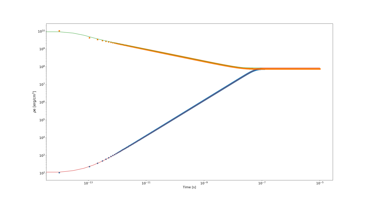
Figure 1.— Approach to thermal equilibrium test problem ( 4.1). The evolution of gas internal energy density is shown for two cases: initial gas energy density of $10^{10}$ erg cm^-3 (upper solid curve and filled square symbols) and initial gas energy density of 100 erg cm^-3 (lower solid curve and filled circle symbols). Solid curves represent the results of our test simulation with RadFLAH and symbols the analytic solutions of Turner & Stone (2001).

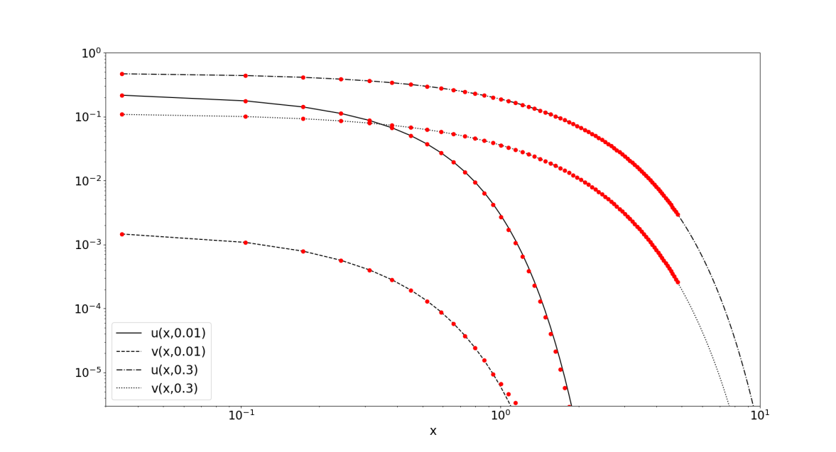
Figure 2.— The non–equilibrium Marshak wave test problem (4.2). Curves represent our numerical results with RadFLAH while filled red circles the analytic results as described by Su & Olson (1996). Dimensionless radiation ($u$) and matter ($v$) energy density is plotted for two choices of dimensionless time: $\tau=$ 0.01 and $\tau=$ 0.3.

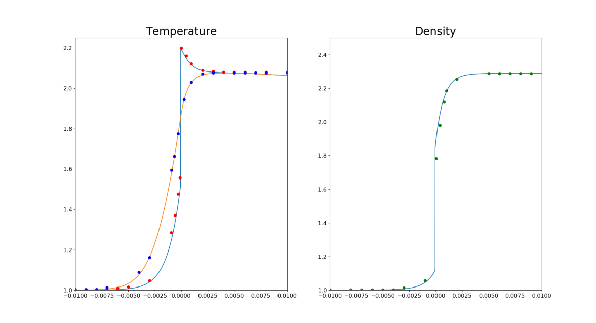
Figure 3.— Temperature (left panel) and density (right panel) profiles for a Mach 2 ($\mathcal{M}=$ 2) subcritical radiative shock (4.3). The orange and blue curves in the left panel correspond to radiation and material temperature respectively.The filled circles correspond to the semi–analytical results of Lowrie & Edwards (2008).

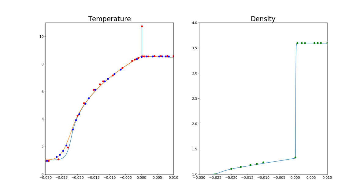
Figure 4.— Same as 3 but for the Mach 5 case ($\mathcal{M}=$ 5).

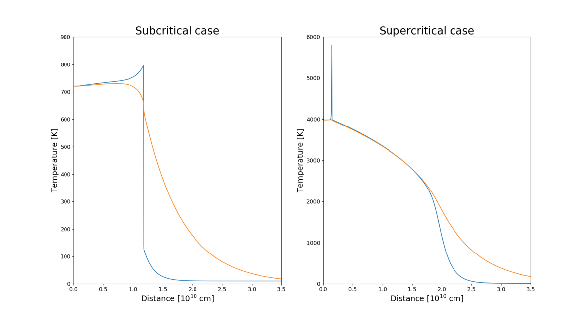
Figure 5.— Radiation (orange curves) and material (blue curves) temperature profiles for a non–steady subcritical radiative shock (left panel, $v_{\rm sh}=$ 6 km s^-1, $t=5.80\times 10^{4}$ s) and a non–steady critical radiative shock (right panel, $v_{\rm sh}=$ 20 km s^-1, $t=5.08\times 10^{3}$ s). Our RadFLAH setup closely follows the one described in Klassen et al. (2014) and comparison against approximate analytical predictions is outlined in (4.4).

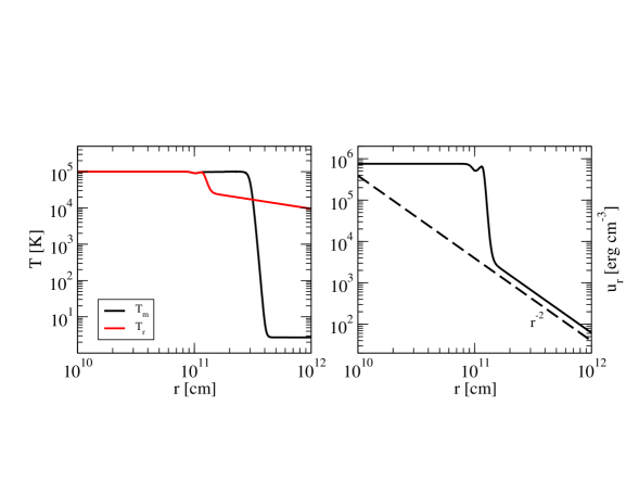
Figure 6.— Profiles of matter ($T_{\rm m}$; solid black curve) and radiation ($T_{\rm r}$; solid red curve) temperature (left panel) and radiation energy density ($u_{\rm r}$; solid black curve, right panel) for the radiating sphere test problem (§ 4.5) at the end of the simulation ($t=10^{6}$ s). The dashed black curve in the right panel denotes a $u_{\rm r}\sim r^{-2}$ decline law.

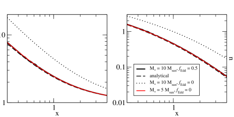
Figure 7.— Profiles of scaled density (left panel) and scaled radial velocity (right panel) for the radiation-inhibited Bondi accretion test problem (§ 4.6) at the end of the simulation ($t=1.538\times 10^{7}$ s or five Bondi times). The solid black and red curves correspond to central source mass of 10 $M_{\odot}$ and 5 $M_{\odot}$ accordingly. The black dashed curve shows the analytic solution and the black dotted curve the case of accretion in the absence of radiation.

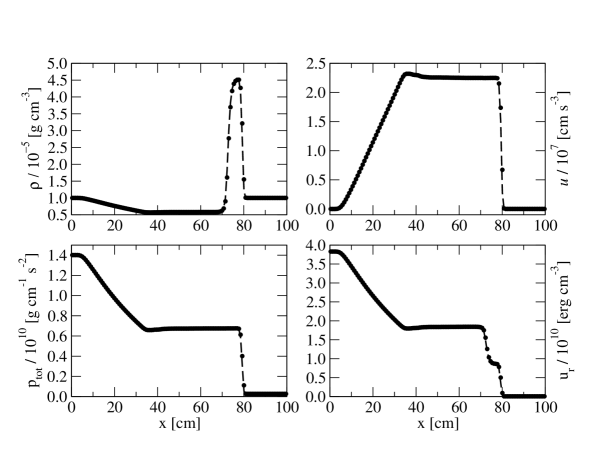
Figure 8.— Profiles of density ($\rho$, upper left panel), velocity ($u$,upper right panel), total pressure ($p_{\rm tot}$, lower left panel) and radiation energy density ($u_{\rm r}$, lower right panel) for the shock-tube problem in the strong coupling limit (§ 4.7) at the end of the simulation ($t=10^{-6}$ sec). Black dashed curves denote the pure hydrodynamics and filled circles the full radiation hydrodynamics simulation.

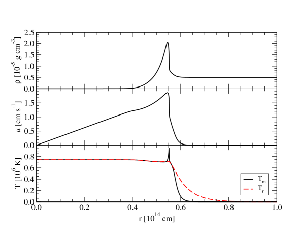
Figure 9.— Profiles of density ($\rho$, upper panel), velocity ($u$, middle panel) and matter ($T_{\rm m}$; black curves) and radiation ($T_{\rm r}$; red curves) temperature (lower panel) for the radiative shock test problem in the weak coupling limit (§ 4.8) at the end of the simulation ($t=10^{6}$ s).

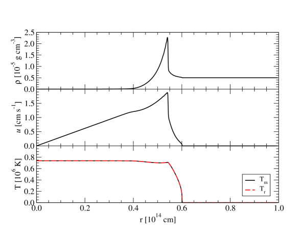
Figure 10.— Same as Figure 9 but for the strong coupling limit (§ 4.8).

4.5. Propagation of radiation front in the optically-thin regime

In this test problem, we examine the capacity of our implementation to correctly calculate the properties of a radiation front streaming in the optically–thin limit and its behavior at large distances from the radiating source, tied to the outer radiation boundary conditions. We initialize our grid with a matter temperature and a density profile given by the sigmoid function:

$$X=X_{\rm s}+\frac{X_{\rm vac}-X_{\rm s}}{1+e^{-\frac{\beta}{r_{\rm*}}(r-r_{\rm*})}},$$ (32)

where $X=\rho,T_{\rm m}$ and the subscripts “vac” and “s” are used for “vacuum” (the outer, optically-thin region of the domain) and “sphere” (the inner, radiating sphere region) accordingly. The parameter $r_{\rm*}$ controls the radius where the profile transitions from the sphere to the vacuum and $\beta$ sets the steepness of this transition. We select $\beta=30$ and $r_{\rm*}=1,3\times 10^{11}$ cm for the $\rho$ and $T_{\rm m}$, accordingly. We allow the temperature profile to break at a larger radius than the density profile in order to probe the effects of radiation matter coupling in the intermediate region. The radiation temperature ($T_{\rm r}$) is initialized to zero throughout the domain in order to force the system to start in an out of equillibrium state. We assume a fully ionized H gas that follows the $\gamma$ law equation of state (EOS) with $\gamma=$ 5/3. We also assume $\rho_{\rm s}=$ 1 g cm^-3, $\rho_{\rm vac}=10^{-9}$ g cm^-3, $T_{\rm s}=10^{5}$ K and $T_{\rm vac}=$ 2.7 K. For the absorption and the transport coefficients, we set $\kappa_{\rm P}=4\times 10^{-10}$ and $\kappa_{\rm R}=4\times 10^{-6}$ cm^-1 accordingly but use the op_constcm2g Opacity implementation in FLASH that adjusts the opacity in a way that depends on the density profile given by Equation 32 (opacity $=\kappa/\rho$, in units of cm² g^-1). For example, deep inside the sphere the transport opacity is $4\times 10^{-6}$ cm² g^-1 (since $\rho_{\rm s}=$ 1 g cm^-3) while far in the vacuum it is $4\times 10^{3}$ cm² g^-1 (since $\rho_{\rm vac}=10^{-9}$ g cm^-3). Our Rosseland and Plack mean opacity choices (1) imply weak coupling between radiation and matter. In addition, the material is optically–thin outside the radius of the radiating sphere.

Figure 6 shows the final state of our simulation ($t=10^{6}$ s). The radiation temperature has fully equillibrated with matter temperature within the optically–thick dense sphere and the radiation energy density ($u_{\rm r}$) declines following a $r^{-2}$ law at large distances. This is consistent with the behavior of radiative flux at large distances from a radiating source (the “inverse–square law”: $u_{\rm r}=L/4\pi r^{2}$, where $L$ is the intrinsic luminosity of the source and $r$ the distance from the center).

4.6. Radiation-inhibited Bondi accretion

To study the dynamical effects of radiation pressure on matter in the optically–thin limit we simulate the process of radiation–inhibited Bondi accretion (Bondi, 1952). A radiating point source of mass $M$ is assumed in the center of the domain, surrounded by a low–density medium. Radiation from the point source free–streams into the surrounding material exerting force on it, causing the inward spherical accretion onto the gravitating mass to decelerate. The magnitude of the specific (per mass) radiating force on the ambient gas is given by the following expression:

$$f_{\rm r}=\frac{\kappa_{R}L}{4\pi r^{2}c},$$ (33)

where $L$ is the luminosity of the point source. The ratio of the radiative to the gravitational force is equal to the fraction of the Eddington luminosity with which the central source is radiating:

$$f_{\rm Edd}=\frac{\kappa_{R}L}{4\pi GMc},$$ (34)

where $G$ the gravitational constant. Radiation inhibits accretion in a way that is equivalent to the gravitational force by a non–radiating point–source with mass $\left(1-f_{\rm Edd}\right)M$. The time–scale for the accretion system to settle is $\simeq r_{\rm B}/c_{\rm s}$ where $r_{\rm B}$ is the Bondi radius ($r_{\rm B}=\left(1-f_{\rm Edd}\right)GM/c_{\rm s}^{2}$) and $c_{\rm s}$ the speed of sound in the ambient medium. Assuming an isothermal gas, analytical solutions for the final density and velocity radial profiles can be found by solving the following system of equations (Shu, 1992):

$$x^{2}\alpha u=\xi$$ (35)

$$\frac{u^{2}}{2}+\ln\alpha-\frac{1}{x}=0,$$ (36)

where $\xi=e^{1.5}/4$ is a constant specific for an isothermal gas, $x=r/r_{\rm B}$ is the dimensionless radius, $\alpha=\rho/\rho_{\rm vac}$ the dimensionless density and $u=v/c_{\rm s}$ the dimensionless velocity.

In this test problem, we use the exact same initial setup as (Krumholz et al., 2007) in order to compare our code with their mixed–frame implementation for radiation hydrodynamics. More specifically, we adopt $\rho_{\rm vac}=10^{-18}$ g cm^-3, $T_{\rm r,vac}=T_{\rm m,vac}=10^{6}$ K corresponding to $c_{\rm s}=1.3\times 10^{7}$ cm s^-1. For the radiating point–source we set $M=$ 10 $M_{\odot}$ and $L=1.6\times 10^{5}$ $L_{\odot}$. Since we are not treating the central source as a sink particle, in contrast with the Krumholz et al. (2007) approach, we employ the Dirichlet option in FLASH for the inner boundary condition for radiation, effectively fixing the radiation and matter temperature in that boundary in a way that it corresponds to the same $L$. We also enforce radiation–matter coupling by setting $\kappa_{\rm P}=$ 0. With this choice of parameters, $f_{\rm Edd}=$ 0.5, meaning that the effects of radiation–inhibited accretion are equivalent to pure accretion onto a non–radiating point–source with mass 5 $M_{\odot}$.

The simulation is run for five Bondi time–scales and the results are shown in Figure 7. We compare accretion with and without radiation included for the original point source, the analytical solution and accretion without radiation included for a point source of half mass (5 $M_{\odot}$). Our results are in very good agreement with the analytical solution and compare well with those of Krumholz et al. (2007) (their Figure 9).

4.7. Shock–Tube problem in the strong coupling limit

To study our implementation in the limit of strong equillibrium and no diffusion we simulate the shock–tube problem. To compare our implementation with results from the CASTRO gray radiation hydrodynamics framework, we use the same initial setup as the one presented in Zhang et al. (2011). We divide an 1D Cartesian grid into two distinct regions, separated in the center of the domain at 50 cm that is coincident with a temperature discontinuity. The initial density is uniform throughout the domain and set to $\rho(x)=10^{-5}$ g cm^-3. The initial velocity is zero everywhere and the initial matter and radiation temperature are set to be equal and initialized in the following way:

$$T_{\rm r,m}=1.5\times 10^{6}\theta(50-x)+3.0\times 10^{5}\theta(x-50),$$ (37)

where $\theta(x-x^{\prime})$ is the unit step function. We assume the gas to be ideal ($\gamma=$ 5/3) with a mean molecular weight $\mu=$ 1. Due to the large values for $\kappa_{\rm P}$, $\kappa_{\rm R}$ (1), matter and radiation are in strong equillibrium and the domain is optically–thick.

Figure 8 shows the final density, velocity, total (radiation plus gas) pressure and radiation energy density. The full radiation hydrodynamics simulation (filled circles) is compared against a pure hydrodynamics simulation that in the strong–coupling limit gives almost identical results because of the fact that the pure hydrodynamic calculation uses an EOS which includes a radiation contribution while the full radiation hydrodynamic calculation does not. Our results are in very good agreement with the results presented in Figure 8 of (Zhang et al., 2011).

4.8. Radiative shock in the weak and strong–coupling limit

Given that radiative blast waves are quite common in astrophysical systems and of direct relevance to SNe, this test problem aims to validate the capacity of our implementation to treat shocks both in the weak and the strong radiation–matter coupling limit. More specifically, we evaluate our two implementations for the treatment of radiation transfer: the flux–limited diffusion solver presented in § 3.2 and the iterative solver for strong radiation–matter coupling (the new ExpRelax implementation in FLASH, § 3.2). The motivation for using ExpRelax in the strong coupling case is to take advantage of the reduced timesteps and stability it offers in this regime and simultaneously test its performance as well. To benchmark against CASTRO we use the same simulation setups as those presented by Zhang et al. (2011). Specifically, we initialize our domain in 1D spherical coordinates and with a constant–density material, $\rho(r)=5\times 10^{-6}$ g cm^-3, at rest ($v(r)=$ 0 cm s^-1) and with a constant radiation and matter temperature set to the same value ($T_{\rm r,m}=$ 1000 K). The shock is initalized in the left (inner) part of the domain by setting both the radiation and matter temperature to $10^{7}$ K for $r\leq 2\times 10^{12}$ cm. This is 10,000 times higher than the temperature in the ambient material. We assume ideal gas ($\gamma=$ 5/3) with $\mu=$ 1. We select our refinement parameters in a way that corresponds to a maximum resolution of $9.766\times 10^{10}$ cm, intermediate between the low and high–resolution cases presented in (Zhang et al., 2011).

In the weak–coupling limit we take the ratio of the emission/absorption to the transport opacity to be $\kappa_{\rm P}/\kappa_{\rm R}=10^{-6}$. In this case, radiation is free to escape in front of the shock forming a radiative precursor and, over time, the radiation and matter temperature depart from equillibrium. In the strong–coupling limit we take the opacity ratio to be $\kappa_{\rm P}/\kappa_{\rm R}=$ 1000. In this case, $T_{\rm r}$ and $T_{\rm m}$ remain in equillibrium throughout the simulation and the result is expected to be identical to the corresponding pure 1–T hydrodynamics case. Figures 9 and 10 show the results at the end of the simulations for the weak–coupling and the strong–coupling case accordingly. Again, a great agreement is reproduced between the results of RadFLAH and those of Zhang et al. (2011).

5. APPLICATION: 1D SUPERNOVA EXPLOSION

In order to illustrate the capacity of RadFLAH to model astrophysical phenomena, we model the LCs of SNe coming from two different progenitor stars: a red supergiant (RSG) star with an extended hydrogen envelope and a more compact star stripped of its hydrogen envelope (“stripped”). The RSG model is expected to produce a Type IIP SN LC with a long ($\sim$ 100 d) plateau phase of nearly constant bolometric luminosity ($L_{\rm bol}$) followed by the late–time decline due to the radioactive decays of ⁵⁶Ni and ⁵⁶Co. The “stripped” model on the other hand, due to the lack of an extended hydrogen envelope and the smaller mass, will produce a fast–evolving LC with an 1-2 week long re–brightening phase due to heating by radioactivity. Our model LCs will be compared against those of the SuperNova Explosion Code (SNEC) (Morozova et al., 2015) using the same input RSG and “stripped” SN profiles.

5.1. Heating due to radioactive decay of ⁵⁶Ni and SN ejecta opacity

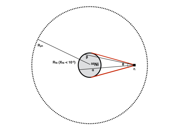
Figure 11.— Illustration of the method used to calculate updated specific internal energy in the star due to heating by the ⁵⁶Ni and ⁵⁶Co radioactive decays. $R_{\rm ph}$ and $R_{\rm Ni}$ refer to the radii of the photosphere and the ⁵⁶Ni sphere respectively defined by the location where $X_{\rm Ni}<10^{-5}$. The zone in location $r_{\rm 1}$ in the SN ejecta is heated by the decay of radioactive material spanning an angle $\theta$. We consider an angular resolution ($\theta/N_{\rm angular}$), where $N_{\rm angular}$ the number of rays extending from the ⁵⁶Ni sphere to $r_{\rm 1}$. For each path (example paths $\alpha$ and $\beta$ are shown, we also consider a “radial resolution”, $N_{\rm radial}$, along the path to sum contributions due to heating from all regions of the ⁵⁶Ni sphere.

A new Heat physics unit was implemented in FLASH to treat the heating of the SN ejecta due to $\gamma$–rays produced by the radioactive decays of ⁵⁶Ni and ⁵⁶Co. The method used to re–calculate the specific internal energy added in each zone is entirely based on Swartz et al. (1995) and it is the same technique incorporated in SNEC and described in the code’s users guide online .

This method involves solving the radiation transfer equation in the gray approximation assuming $\gamma$–ray opacity, $\kappa_{\rm\gamma}=0.06Y_{\rm e}$ cm² g^-1, where $Y_{\rm e}$ is the electron fraction. The algorithm loops through all radial zones and calculates the integrated intensity of radiation coming from paths originating from a central spherical region where ⁵⁶Ni is concentrated (Figure 11). To determine the radius of the ⁵⁶Ni sphere we set a threshold on the ⁵⁶Ni mass fraction of $10^{-5}$. We then define a radial ($N_{\rm radial}$) resolution along each path and an angular ($N_{\rm angular}$) resolution that determines the number of paths originating from the ⁵⁶Ni sphere that contribute to the heating of each zone. For the models discussed later we use $N_{\rm radial}=N_{\rm angular}=$ 100. Finally, the internal energy of each zone is updated accordingly by adding that extra heating source term. To preserve a fast running–time, we only add the radioactive decay heating periodically, every one day (86,400 s) throughout the run.

Given our objective to model radiation diffusion through SN ejecta, a new FLASH Opacity was developed that takes advantage of the Lawrence Livermore National Laboratory (LANL) OPAL opacity database (Iglesias & Rogers, 1996). We specifically used opacity tables in two temperature regimes: the low ($\log T<4.5$; Ferguson et al. 2005) and the high–temperature ($\log T>4.5$; Grevesse & Sauval 1998) regime based on solar metal abundances. We directly linked the OPAL tables from the stellar evolution MESA code opacity database in order to take advantage of the consistent and succinct formatting in these files. This way, all values for the Rosseland mean opacity directly correspond to the OPAL values for each zone in the initialization of the supernova runs. For the Planck mean opacity, on the other hand, we adopted a fiducial constant value by assuming Thompson scattering as the main source of opacity. As such, for the (H–rich) “RSG” run we have used $\kappa_{\rm P}=$ 0.4 cm² g^-1 and for the (H–poor) “stripped” run $\kappa_{\rm P}=$ 0.2 cm² g^-1. In order to be provided with a robust comparison against the results of SNEC, we had to impose their adopted opacity floor given by:

$$\kappa_{\rm floor}(r)=\frac{0.24Z_{\rm env}-0.01-0.23Z(r)}{Z_{\rm env}-1},$$ (38)

where $Z_{\rm env}$ is the metallicity of the stellar envelope and $Z(r)$ the metallicity as a function of radius.

5.2. Input SN ejecta profiles

Figure 12 shows the initial structural properties ($\rho$, $T$ and composition) of the basic RSG and “stripped models used taken from the available profiles within the SNEC source tree (15Msol_RSG and stripped_star therein). In SNEC it is emphasized that these models were evolved to the pre–SN stage using the MESA code. The RSG model represents a red supergiant star that was 15 $M_{\odot}$ at Zero Age Main Sequence (ZAMS) while the “stripped model a compact blue star from a 15 $M_{\odot}$ ZAMS model where the convective envelope was stripped during the evolution (Piro & Morozova, 2014). Considering mass–loss during the evolution, the final, pre–explosion models had total masses of 12.2 $M_{\odot}$ (RSG) and 4.9 $M_{\odot}$ (“stripped”).

SNEC provides the user with the option to set a total ⁵⁶Ni mass as an input and the option to apply one–dimensional parameterized mixing due to the Rayleigh–Taylor and Richtmyer–Meshkov instabilities the SN ejecta using the boxcar smoothing method (Kasen & Woosley, 2009). In order to investigate these effects we run three SNEC models for each progenitor: one with $M_{\rm Ni}=$ 0.05 $M{\odot}$ using the original SN ejecta profiles, one with $M_{\rm Ni}=$ 0.05 $M{\odot}$ but with boxcar smoothing applied, and one with no ⁵⁶Ni radioactive decay contributions for a total of six SNEC models. For all three RSG’ models and the “stripped” model with boxcar mixing applied run in SNEC, we extract density, temperature and velocity profiles at a time prior to SN shock break–out and when the shock front is a few tenths of a solar mass within the photosphere (taken to be at optical depth of 2/3). Also, since SNEC does not use nuclear reaction networks and no nucleosynthesis is performed after the explosion, the initial input model abundance profiles are assumed fixed except for the models for which modifications were applied using boxcar averaging. All SNEC pre–SN break–out profiles are then mapped into the 1D Adaptive Mesh Refinement (AMR) grid of FLASH and their evolution is modeled using the RadFLAH implementation yielding the computation of gray LCs. We note that in the latest release of RadFLAH we have also included the capability for the user to initiate a “thermal bomb”–driven explosion in the inner regions of the initial SN profile without having to do that step within another code like SNEC.

For the FLASH simulations we used a simulation box of length $4\times 10^{16}$ cm, large enough to follow the expansion of the SN ejecta for a few hundred days. For this reason we had to inlcude a low–mass circumstellar wind with density scaling as $r^{-2}$ outside the star. The temperature of the wind was kept constant at 100 K and the composition was taken to be the same as that of the outer zone of the stellar model. The wind was constructed by assuming a mass–loss rate of $10^{-5}$ $M_{\odot}$ yr^-1 and a wind velocity of 250 km s^-1. The density of the wind followed an $\sim r^{-2}$ profile consistent with the observed properties of RSG–type winds (see Figure 3 in Smith (2014)). The presence of wind material around the SN progenitor makes the effects of the interaction between the SN ejecta and that wind inevitable, yet minimized in our runs given the relatively low wind density and total mass. For a more thorough review on the effects of pre–SN winds for high mass–loss rates ($>10^{-4}$ $M_{\odot}$ yr^-1) on the LCs of SNe the reader is encouraged to review (Moriya et al., 2014). To calculate the bolometric gray LCs in RadFLAH, a photosphere–locating algorithm was employed that tracks the location of the optical depth $\tau=$ 2/3 surface over time and uses the local conditions there to estimate the emergent luminosity.

5.3. SN lightcurves with RadFLAH

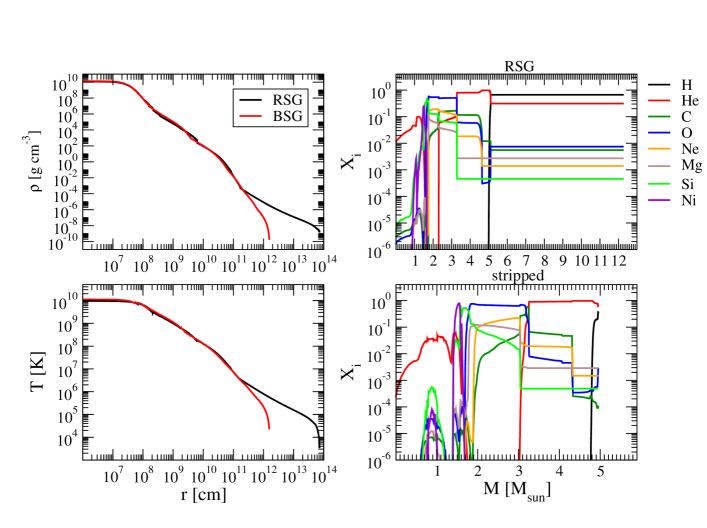
Figure 12.— The inital SN profiles used for the calculation of gray LCs with FLASH RadFLAH. Density (upper left panel) and temperature (lower left panel) for the RSG (black curves) and “stripped” (red curves) models. Composition profiles for the RSG (upper right panel) and the “stripped” (lower right panel) models where no boxcar mixing is applied (5.2).

Figure 13 shows comparisons between the SNEC and FLASH RadFLAH LCs for the RSG (upper panels) and “stripped” (lower panels) models. The left panels are a zoom–in to the early shock break–out and “fireball” expansion phase while the right panels show the total LC evolution, including re–heating of the SN ejecta due to the radioactive decay of ⁵⁶Ni. The comparison between the shock–breakout LCs indicates that the FLASH RadFLAH models exhibit a less luminous yet longer–lasting break–out phase for both the RSG and “stripped” model, although the total radiated energy is about the same. These differences are attributed to two factors. First and foremost, the two–temperature (2T) treatment where we allow the material and radiation temperature to de–couple in RadFLAH while there is just one combined temperature used in SNEC. During shock break–out in SNe, 2T effects are strong in the weak coupling limit (see also 4.8). This includes the effect of a radiative precursor leaking ahead of the shock and heating the surrounding medium thus driving the radiation temperature at the photosphere to lower values. Secondly, in contrast with the SNEC setup we include a low–density wind around the star that can also influence the properties of shock brek–out emission.

The later, re–brightening phases due to the deposition of gamma–rays to the SN ejecta by ⁵⁶Co decay are in good agreement with the SNEC results for both models. The $\sim$ 100 d plateau phase for the RSG models is reproduced at a luminosity of $\sim$ $3\times 10^{42}$ erg s^-1 that is typical for Type IIP SN LCs. Also, the late–time ($>$ 100 d) radioactive decay tail that has a characteristic constant decline rate for ⁵⁶Co is reproduced and is consistent with the SNEC results. For the RSG model with $M_{\rm Ni}=$ 0 there are considerable differences between the SNEC and FLASH RadFLAH results at late times after the plateau, with the FLASH RadFLAH models exhibiting a much faster decline in luminosity. The FLASH RadFLAH result is more in line with the predictions of analytical models for Type IIP LCs like that of Arnett & Fu (1989), given that the effective opacity drops to zero after the end of the hydrogen recombination phase and luminosity should quickly decline during the nebular phases. Similar “tail–less” Type IIP SN LC models in the context of pulsational pair–instability explosions from massive progenitor stars were computed by Woosley (2017) featuring rapid decline rates once the hydrogen recombination front recedes inwards. Another source of this discrepancy is the post–plateau opacities adopted in the SNEC code attempting to take into account effects due to dust formation in the SN ejecta at late times and low–temperature conditions (Ferguson & Dotter, 2008).

The “stripped” LC models are also in good agreement between the two codes and are characterized by a faster LC evolution attributable to the smaller initial radius and envelope mass for these progenitors. The same effect of a more smeared–out shock break–out LC is observed here as was the case for the “RSG” model but the later evolution and the ⁵⁶Ni decay tail are in great agreement between SNEC and FLASH RadFLAH.

Given the many differences in the treatment of radiation diffusion between the two codes, the initial setup requiring the presence of a circumstellar wind in FLASH and discrepancies in the overall numerical implementation, the agreement between the two codes is intriguing and illustrates the capacity of the new RadFLAH implementation to provide basic 2T modeling for explosive astrophysical flows including SNe and interaction of SN ejecta with circumstellar matter (CSM).

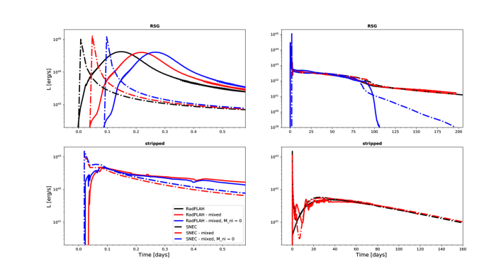
Figure 13.— Comparison between FLASH RadFLAH (solid curves) and SNEC (dashed curves) SN LCs. The upper panels show the results for the “RSG” models and the lower panels those for those “stripped” model. The left panels show a 0.8 day zoom–in the early shock–breakout LCs while the right panels the full LC. The agreement between the two codes is reasonably good given differences in the numerical treatment of radiation diffusion and microphysics.

6. DISCUSSION

The multi–physics, multi–dimensional AMR code FLASH has been used for studies of the hydrodynamics of astrophysical systems extensively in the past (Calder, 2005; Chatzopoulos et al., 2013; Couch & Ott, 2013; Chatzopoulos et al., 2014; Klassen et al., 2014; Couch & Ott, 2015; Couch et al., 2015; Chatzopoulos et al., 2016; Klassen et al., 2016). Although a three–temperature (electron, ion and radiation temperature) radiation diffusion scheme was already present in FLASH, it was tailored for the treatment of high energy density and laser physics problems and direct application for physical regimes that are appropriate for astrophysical objects like supernovae was not feasible.

For this reason, we extended the hydrodynamics capabilities of the unsplit hydrodynamics solver available in FLASH and implemented the new Radiation Flux–limiter Aware Hydrodynamics (RadFLAH) framework able to treat astrophysical problems by evolving the radiation and matter separately in a two–temperature approach and in the gray approximation using the Levermore–Pomraning approximation for the flux limiter.

To be able to utilize our method for astrophysical applications, we implemented an extension of the existing “Helmholtz” equation of state in FLASH to lower temperature and density regimes characteristic of stellar photospheres and circumstellar environments. We also introduced a new opacity unit linking the OPAL opacity database to obtain transport opacity values as a function of local temperature, density and composition. Finally, we introduced a commonly–used method to treat the deposition of gamma–rays to the SN ejecta due to the ⁵⁶Co and ⁵⁶Ni radioactive decay heating as necessary in order to calculate complete SN LCs to late times after the explosion.

We compared FLASH RadFLAH to flux–limited diffusion implementation used in other codes like CASTRO (Zhang et al., 2011) and the Krumholz et al. (2007) code as well as analytical solutions by running standard radiation hydrodynamics and radiation diffusion test problems identical to some of those presented in their methods papers and found very consistent results. Finally, we performed a direct code–to–code comparison with the Supernova Explosion Code (SNEC Morozova et al. (2015)) in order to assess our computed SN LCs for two modes: a red supergiant progenitor with an extended hydrogen envelope and a more compact blue supergiant progenitor that experienced strong mass–loss during its evolution, originally performed with the MESA stellar evolution code. Given differences in the numerical treatment of hydrodynamics (two–temperture in RadFLAH versus one–temperature in SNEC) and radiation transfer as well as initial setup (in FLASH we had to use a large simulation box and provide data for a low–density circumstellar wind around the progenitor star models), RadFLAH LCs were consistent with those computed by SNEC for the same inital SN profiles. More specifically, we were able to reproduce the characteristics of the main (post break–out) and late–time (radioactive decay “tail”) phase for both models very well. The differences due to our two–temperature treatment and the existence of a low–density wind around the progenitor causing some SN ejecta–circumstellar matter interaction effects, are more prevalent during the early bright shock–break out phase of the LCs. More specifically, we computed shock–break out LCs that reach lower peak luminosities and last longer than the ones found by SNEC, yet the total radiated energy throughout this early burst remained consistent.

6.1. Applicability of RadFLAH approach

The RadFLAH method is applicable to a variety of astrophysical radiation hydrodynamics problems beyond simple SN LC computations like, for example, studies of SN ejecta–CSM interaction. In a future release we plan to expand the RadFLAH capabilities to treat problems in two and three dimensions and for different geometries as well as to incorporate a multi–group treatment for radiation diffusion allowing the user to compute band–specific SN LCs. Given the open access to the public release of the FLASH code and its popularity amonst numerical astrophysicists, we hope that this new, open framework finds good use in the community.

Based on the associated approximations and assumptions, we expect our method to be particularly useful in regimes that are either close to diffusive or close to free–streaming. The accuracy and stability of the method under conditions of dynamical diffusion (for example, when $v/c<<1$ does not apply) has not been examined and should not be assumed. We expect the method to give good solutions in diffusion–dominated and free–streaming regions of a simulation domain; and to sensibly connect such different regions if they exist. We do not expect the solution to particularly good in regions that cannot be viewed as close to either (statically) diffusive or free–streaming radiation.

Stability of simulations is not always given, in particular due to the time–lagged handling of some quantities in the equations (in particular the flux limiter $\lambda$). This is subject to further research.

APPENDIX

To discuss our implementation in more detail, in a 2T(M+R) formulation, we write our state in (mostly) conservative form as introduced above,

$${\mathitbf{U}}=\begin{pmatrix}\rho\cr\rho{\mathitbf{v}}\cr E_{\mathrm{tot}}\cr\rho e_{\mathrm{m}}\cr E_{\mathrm{r}}\cr X_{1}\rho\cr\vdots\cr X_{n}\rho\end{pmatrix}$$ (39)

and our evolution equations as

$$\frac{\partial}{\partial t}{\mathitbf{U}}=f_{hyperbolic}+f_{fixup1}+f_{fixup2}+f_{Lorentz}+f_{transp}\,.$$ (40)

To allow for different choices for the implementation of some terms, and allow for parametric control of these for the purpose of experimentation, we introduce numerical parameters $\alpha_{\mathrm{m}},\alpha_{\mathrm{r}},\beta_{\mathrm{m}},\beta_{\mathrm{r}}\in[0,1]$. These control, separately for both matter and radiation components of energy, whether (and, if we allow them to have non-integer values, to what degree):

• pressure terms are included in the conservative fluxes ($\alpha_{\rm m,r}$),

• work terms are implemented explicitly ($\beta_{\rm m,r}$),

and we require

$$\alpha_{c}+\beta_{c}\leq 1\quad\mbox{for $c\in\{{\mathrm{m}},{\mathrm{r}}\}$}.$$

In case we want the dominant changes of $E_{\mathrm{m}},E_{\mathrm{r}}$ that go beyond simple advection to be completely represented by explicit terms in $f_{hyperbolic}$ and $f_{fixup1}$, we have to set $\alpha_{c}+\beta_{c}=1$. If, on the other hand, we want those changes to be handled by the $f_{fixup2}$ term, we set $\alpha_{c}=\beta_{c}=0$. For the tests presented in this paper, we have typically chosen either the latter or $\beta_{r}=$ 0, $\beta_{m}=$ 1, $\alpha_{m}=$ 0, $\alpha_{r}=$ 1.

Then

$$f_{hyperbolic}=\begin{pmatrix}-\nabla\cdot(\rho{\mathitbf{v}})\cr-\nabla\cdot(\rho{\mathitbf{v}}{\mathitbf{v}})-\nabla p-\lambda\nabla E_{\mathrm{r}}\cr-\nabla\cdot\left[(E_{\mathrm{tot}}+P_{\mathrm{tot}}+p_{\Lambda}){\mathitbf{v}}\right]\cr-\nabla\cdot\left(\rho e_{\mathrm{m}}{\mathitbf{v}}+\alpha_{\mathrm{m}}p{\mathitbf{v}}\right)\cr-\nabla\cdot\left[(1+\alpha_{\mathrm{r}}\lambda)E_{\mathrm{r}}{\mathitbf{v}}+p_{\Lambda}{\mathitbf{v}}\right]\cr-\nabla\cdot(\rho X_{1}{\mathitbf{v}})\cr\vdots\cr-\nabla\cdot(\rho X_{n}{\mathitbf{v}})\cr\end{pmatrix},$$ (41)

$$f_{fixup1}=\begin{pmatrix}0\cr\mathbf{0}\cr 0\cr-\beta_{\mathrm{m}}p\,\nabla\cdot{\mathitbf{v}}+\alpha_{\mathrm{m}}{\mathitbf{v}}\cdot\nabla p\cr-\beta_{\mathrm{r}}\lambda E_{\mathrm{r}}\,\nabla\cdot{\mathitbf{v}}-(1-\alpha_{\mathrm{r}})\left(E_{\mathrm{r}}{\mathitbf{v}}\cdot\nabla\lambda\right)+\,\alpha_{\mathrm{r}}\lambda\,{\mathitbf{v}}\cdot\nabla E_{\mathrm{r}}\cr 0\cr\vdots\cr 0\end{pmatrix},$$ (42)

$$f_{fixup2}=\begin{pmatrix}0\cr\mathbf{0}\cr 0\cr w_{\mathrm{m}}\cr w_{\mathrm{r}}\cr 0\cr\vdots\cr 0\end{pmatrix},$$ (43)

Here we have introduced “work-like” quantities $w_{m}$ and $w_{r}$ that represent any changes in the thermal and radiation energies that are not already included in the explicit terms of $f_{hyperbolic}+f_{fixup1}$. In numerical application, we first apply the updates $f_{hyperbolic}+f_{fixup1}$ terms to a discretized version of $\mathitbf{U}^{n}$ at a time $t_{n}$ to compute an intermediate state:

$${\mathitbf{\widetilde{U}}}^{n+1}=\mathitbf{U}^{n}+(f_{hyperbolic}+f_{fixup1})\,\Delta t.$$

This is done by first using a (slightly modified) traditional Godunov method for a conservative update as per $f_{hyperbolic}$, and then applying additional terms. An important modification is the $-\lambda\nabla E_{\mathrm{r}}$ term in the momentum equation. We currently use precomputed $\lambda^{n}$ values based on the previous time step in the implementation, represented on the same discrete grid used for cell-centered conservative variables. We have implemented numerical spatial smoothing of this flux-limiter variable to counteract instabilities that we found in some simulations.

For the components of $\mathitbf{U}^{n}$ we have $E_{\mathrm{tot}}=\rho e_{\mathrm{m}}+E_{\mathrm{r}}+\rho\frac{{\mathitbf{v}}^{2}}{2}$, this will in general not be true for the components of ${\mathitbf{\widetilde{U}}}^{n+1}$, and we compute the energy mismatch

$$\Delta E_{\mathrm{tot}}=\widetilde{E_{\mathrm{tot}}}-\left(\tilde{\rho}\tilde{e_{\mathrm{m}}}+\tilde{E_{\mathrm{r}}}+\tilde{\rho}\frac{{\mathitbf{\tilde{\mathitbf{v}}}}^{2}}{2}\right),$$

where tilde indicates components of ${\mathitbf{\widetilde{U}}}^{n+1}$.

Next we reestablish consistency between the energy components by applying the $f_{fixup2}$ term. Note that we trust the value of $\widetilde{E_{\mathrm{tot}}}$ (as well as $\tilde{\rho}$ and ${\mathitbf{\tilde{\mathitbf{v}}}}^{2}$), which come from the conservative update of the hyperbolic system, more than the updated values of $\tilde{e_{\mathrm{m}}}$ and $\tilde{E_{\mathrm{r}}}$, so we adjust the latter by partitioning the energy mismatch among then, such that $\Delta E_{\mathrm{tot}}=\left(w_{\mathrm{m}}+w_{\mathrm{r}}\right)\Delta t$. We have implemented various strategies for effecting this partitioning. We briefly describe here “RAGE-like energy partitioning” (RLEP), which is based on the same approach that has been implemented in the FLASH code (Release 4 and later) for partitioning of energies between electron and ion components, which in turn is described in Gittings et al. (2008).

Let $q_{c}=w_{c}\Delta t$ for $c\in\{{\mathrm{m}},{\mathrm{r}}\}$. Let $p^{+}$, $P_{\mathrm{rad\,eff}}^{+}=\lambda\tilde{E_{\mathrm{r}}}$, and $P_{\mathrm{tot}}^{+}=p^{+}+P_{\mathrm{rad\,eff}}^{+}$ be predicted values of matter, effective radiation, and total pressures, respectively, at time $t_{n+1}$ that can be computed by Eos calls on the ${\mathitbf{\widetilde{U}}}^{n+1}$ state. Then define

$$q_{\mathrm{m}} = \frac{p^{+}}{P_{\mathrm{tot}}^{+}}\Delta E_{\mathrm{tot}},\quad q_{\mathrm{r}}=\frac{P_{\mathrm{rad\,eff}}^{+}}{P_{\mathrm{tot}}^{+}}\Delta E_{\mathrm{tot}},$$ (44)

i.e., simply partition the energy mismatch in proportion to the pressure ratios. We also use additional fallbacks and heuristics, e.g., to recover from unphysical nonpositive energy values.

References

- Arnett & Fu (1989) Arnett, W. D., & Fu, A. 1989, ApJ, 340, 396
- Blinnikov et al. (1998) Blinnikov, S. I., Eastman, R., Bartunov, O. S., Popolitov, V. A., & Woosley, S. E. 1998, ApJ, 496, 454
- Bondi (1952) Bondi, H. 1952, MNRAS, 112, 195
- Calder (2005) Calder, A. C. 2005, Ap&SS, 298, 25
- Calder et al. (2004) Calder, A. C., Plewa, T., Vladimirova, N., Lamb, D. Q., & Truran, J. W. 2004, Astrophysical Journal, Letters, submitted
- Castor (2007) Castor, J. I. 2007, Radiation Hydrodynamics (Cambridge University Press)
- Chatzopoulos et al. (2016) Chatzopoulos, E., Couch, S. M., Arnett, W. D., & Timmes, F. X. 2016, ApJ, 822, 61
- Chatzopoulos et al. (2014) Chatzopoulos, E., Graziani, C., & Couch, S. M. 2014, arXiv preprint arXiv:1405.4873
- Chatzopoulos et al. (2014) Chatzopoulos, E., Graziani, C., & Couch, S. M. 2014, ApJ, 795, 92
- Chatzopoulos et al. (2013) Chatzopoulos, E., Wheeler, J. C., & Couch, S. M. 2013, The Astrophysical Journal, 776, 129
- Chatzopoulos et al. (2013) Chatzopoulos, E., Wheeler, J. C., & Couch, S. M. 2013, ApJ, 776, 129
- Clarke (1996) Clarke, D. A. 1996, ApJ, 457, 291
- Colella & Glaz (1985) Colella, P., & Glaz, H. M. 1985, Journal of Computational Physics, 59, 264
- Commerçon et al. (2011) Commerçon, B., Teyssier, R., Audit, E., Hennebelle, P., & Chabrier, G. 2011, A&A, 529, A35
- Couch (2013a) Couch, S. M. 2013a, The Astrophysical Journal, 765, 29
- Couch (2013b) —. 2013b, The Astrophysical Journal, 775, 35
- Couch et al. (2015) Couch, S. M., Chatzopoulos, E., Arnett, W. D., & Timmes, F. X. 2015, ApJL, 808, L21
- Couch & O’Connor (2013) Couch, S. M., & O’Connor, E. P. 2013, arXiv preprint arXiv:1310.5728
- Couch & Ott (2013) Couch, S. M., & Ott, C. D. 2013, ApJL, 778, L7
- Couch & Ott (2015) —. 2015, ApJ, 799, 5
- Dubey et al. (2012) Dubey, A., Daley, C., ZuHone, J., Ricker, P. M., Weide, K., & Graziani, C. 2012, ApJS, 201, 27
- Ensman (1994) Ensman, L. 1994, ApJ, 424, 275
- Ferguson et al. (2005) Ferguson, J. W., Alexander, D. R., Allard, F., Barman, T., Bodnarik, J. G., Hauschildt, P. H., Heffner-Wong, A., & Tamanai, A. 2005, ApJ, 623, 585
- Ferguson & Dotter (2008) Ferguson, J. W., & Dotter, A. 2008, in IAU Symposium, Vol. 252, The Art of Modeling Stars in the 21st Century, ed. L. Deng & K. L. Chan, 1–11
- Ferland et al. (1998) Ferland, G. J., Korista, K. T., Verner, D. A., Ferguson, J. W., Kingdon, J. B., & Verner, E. M. 1998, PASP, 110, 761
- Frey et al. (2013) Frey, L. H., Even, W., Whalen, D. J., Fryer, C. L., Hungerford, A. L., Fontes, C. J., & Colgan, J. 2013, ApJS, 204, 16
- Fryxell et al. (2000) Fryxell, B., et al. 2000, ApJS, 131, 273
- Gittings et al. (2008) Gittings, M., et al. 2008, Computational Science and Discovery, 1, 015005
- González et al. (2007) González, M., Audit, E., & Huynh, P. 2007, A&A, 464, 429
- Grevesse & Sauval (1998) Grevesse, N., & Sauval, A. J. 1998, Space Sci. Rev., 85, 161
- Hauschildt (1992) Hauschildt, P. H. 1992, J. Quant. Spec. Radiat. Transf., 47, 433
- Hauschildt & Baron (1999) Hauschildt, P. H., & Baron, E. 1999, Journal of Computational and Applied Mathematics, 109, 41
- Hauschildt & Baron (2004) —. 2004, A&A, 417, 317
- Hayes & Norman (2003) Hayes, J. C., & Norman, M. L. 2003, ApJS, 147, 197
- Hillier & Dessart (2012) Hillier, D. J., & Dessart, L. 2012, MNRAS, 424, 252
- Iglesias & Rogers (1996) Iglesias, C. A., & Rogers, F. J. 1996, ApJ, 464, 943
- Kasen et al. (2006) Kasen, D., Thomas, R. C., & Nugent, P. 2006, ApJ, 651, 366
- Kasen & Woosley (2009) Kasen, D., & Woosley, S. E. 2009, ApJ, 703, 2205
- Kerzendorf & Sim (2014) Kerzendorf, W. E., & Sim, S. A. 2014, MNRAS, 440, 387
- Klassen et al. (2014) Klassen, M., Kuiper, R., Pudritz, R. E., Peters, T., Banerjee, R., & Buntemeyer, L. 2014, ApJ, 797, 4
- Klassen et al. (2016) Klassen, M., Pudritz, R. E., Kuiper, R., Peters, T., & Banerjee, R. 2016, ApJ, 823, 28
- Krumholz et al. (2007) Krumholz, M. R., Klein, R. I., McKee, C. F., & Bolstad, J. 2007, ApJ, 667, 626
- Levermore & Pomraning (1981) Levermore, C. D., & Pomraning, G. C. 1981, ApJ, 248, 321
- Lowrie & Edwards (2008) Lowrie, R. B., & Edwards, J. D. 2008, Shock Waves, 18, 129
- Mihalas & Mihalas (1984) Mihalas, D., & Mihalas, B. W. 1984, Foundations of radiation hydrodynamics (Oxford University Press)
- Minerbo (1978) Minerbo, G. N. 1978, J. Quant. Spec. Radiat. Transf., 20, 541
- Moriya et al. (2014) Moriya, T. J., Maeda, K., Taddia, F., Sollerman, J., Blinnikov, S. I., & Sorokina, E. I. 2014, MNRAS, 439, 2917
- Morozova et al. (2015) Morozova, V., Piro, A. L., Renzo, M., Ott, C. D., Clausen, D., Couch, S. M., Ellis, J., & Roberts, L. F. 2015, ApJ, 814, 63
- Paxton et al. (2011) Paxton, B., Bildsten, L., Dotter, A., Herwig, F., Lesaffre, P., & Timmes, F. 2011, ApJS, 192, 3
- Paxton et al. (2013) Paxton, B., et al. 2013, ApJS, 208, 4
- Paxton et al. (2015) —. 2015, ApJS, 220, 15
- Piro & Morozova (2014) Piro, A. L., & Morozova, V. S. 2014, ApJL, 792, L11
- Pomraning (1979) Pomraning, G. C. 1979, J. Quant. Spec. Radiat. Transf., 21, 249
- Roth & Kasen (2015) Roth, N., & Kasen, D. 2015, ApJS, 217, 9
- Shu (1992) Shu, F. H. 1992, The physics of astrophysics. Volume II: Gas dynamics. (University Science Books)
- Smith (2014) Smith, N. 2014, ARAA, 52, 487
- Stone et al. (1992) Stone, J. M., Mihalas, D., & Norman, M. L. 1992, ApJS, 80, 819
- Su & Olson (1996) Su, B., & Olson, G. L. 1996, J. Quant. Spec. Radiat. Transf., 56, 337
- Swartz et al. (1995) Swartz, D. A., Sutherland, P. G., & Harkness, R. P. 1995, ApJ, 446, 766
- Townsley et al. (2007) Townsley, D. M., Calder, A. C., Asida, S., Seitenzahl, I. R., Peng, F., Vladimirova, N., Lamb, D. Q., & Truran, J. W. 2007, Astrophysical Journal, 668, 1118+
- Turner & Stone (2001) Turner, N. J., & Stone, J. M. 2001, ApJS, 135, 95
- van der Holst et al. (2011) van der Holst, B., et al. 2011, ApJS, 194, 23
- van Rossum (2012) van Rossum, D. R. 2012, ApJ, 756, 31
- Wise & Abel (2011) Wise, J. H., & Abel, T. 2011, MNRAS, 414, 3458
- Wollaeger et al. (2013) Wollaeger, R. T., van Rossum, D. R., Graziani, C., Couch, S. M., Jordan, IV, G. C., Lamb, D. Q., & Moses, G. A. 2013, ApJS, 209, 36
- Woosley (2017) Woosley, S. E. 2017, ApJ, 836, 244
- Zhang et al. (2011) Zhang, W., Howell, L., Almgren, A., Burrows, A., & Bell, J. 2011, ApJS, 196, 20
- Zhang et al. (2013) Zhang, W., Howell, L., Almgren, A., Burrows, A., Dolence, J., & Bell, J. 2013, ApJS, 204, 7