Simulating a Topological Transition in a Superconducting Phase Qubit by Fast Adiabatic Trajectories

Abstract

The significance of topological phases has been widely recognized in the community of condensed matter physics. The well controllable quantum systems provide an artificial platform to probe and engineer various topological phases. The adiabatic trajectory of a quantum state describes the change of the bulk Bloch eigenstates with the momentum, and this adiabatic simulation method is however practically limited due to quantum dissipation. Here we apply the ‘shortcut to adiabaticity’ (STA) protocol to realize fast adiabatic evolutions in the system of a superconducting phase qubit. The resulting fast adiabatic trajectories illustrate the change of the bulk Bloch eigenstates in the Su-Schrieffer-Heeger (SSH) model. A sharp transition is experimentally determined for the topological invariant of a winding number. Our experiment helps identify the topological Chern number of a two-dimensional toy model, suggesting the applicability of the fast adiabatic simulation method for topological systems.

Introduction
The study of topological phases has been an emerging field in condensed matter physics since the discovery of the integer quantum Hall effect klitzingPRL80 . In the traditional Landau theory of phase transition, each phase is characterized by an order parameter. Instead, various phases in a topological material are distinguished by their different topological invariants. In the theory of Thouless, Kohmoto, Nightingale and den Nijs, the integer Chern number is a topological invariant to interpret a quantized Hall conductivity of a two-dimensional (2D) electronic gas ThoulessPRL82 . Similar topological invariants are defined in other topological systems. For the one-dimensional (1D) Su-Schrieffer-Heeger (SSH) model SSHmodel79 , the topologically nontrivial phase with edge states is characterized by a unity winding number of the bulk structure according to the bulk-boundary correspondence Asboth2016short .

The rapid progress of quantum manipulation techniques has attracted much attention of simulating topological phases using controllable quantum systems, such as cold atoms, superconducting qubits and nitrogen-vacancy (NV) center in diamond  KitagawaNatCommu11 ; AtalaNatPhy13 ; JotzuNat14 ; AidelsburgerNatPhys15 ; DucaSci15 ; MittalNatPhoton16 ; FlaschnerSci16 ; GoldmanNatPhys16 ; RoushanNat14 ; SchroerPRL14 ; Flurin2016 ; KongFeiPRL16 . For the SSH model and other two-band systems, the bulk Hamiltonian in the momentum space is equivalently described by a spin-half particle subject to a changing magnetic field. An adiabatic trajectory of the spin simulates the bulk Bloch eigenstates as the momentum traverses the first Brillouin zone (FBZ). The topological invariant of a Bloch band is subsequently obtained by integrating a local geometric quantity over the closed area of the FBZ ThoulessPRL82 ; Asboth2016short ; HasanRMP10 . The key of this adiabatic simulation is to realize the adiabatic evolution of a quantum state, which is also relevant in quantum information and quantum computation Farhi2000 ; ChuangBook .

However, a slow adiabatic operation is practically challenging since the surrounding environment inevitably destroys quantum coherence at a long time scale. Several strategies have been proposed to speed-up the operation while maintaining adiabaticity DemirplakJPCA03 ; Berry2009 ; XiChenPRL10 ; Masuda2009 ; Torrontegui2013ShortcutReview ; TorosovPRL11 ; MartinisPRA14 . The ‘shortcut to adiabaticity’ (STA) protocol is a general methodology, in which a counter-diabatic Hamiltonian cancels the non-adiabatic deflection of a quantum state DemirplakJPCA03 ; Berry2009 ; XiChenPRL10 ; Masuda2009 ; Torrontegui2013ShortcutReview . The STA protocol has been implemented in a few quantum systems, such as cold atoms and a nitrogen-vacancy center in a diamond BasonNatPhys12 ; JFZhangPRL13 ; ZhouNatPhys16 ; AnNatCommu16 . In a recent experiment, we applied the STA protocol to make a fast measurement of the Berry phase in a superconducting phase qubit ZZXPRA17 .

In this article, we simulate the topological transition of the SSH model based on fast adiabatic trajectories of a superconducting phase qubit under the STA protocol. To remove the influence of higher excited states, the fast adiabatic state transfer is improved by the derivative removal by adiabatic gates (DRAG) method MotzoiPRL09 ; GambettaPRA11 ; Lucero10 . To simulate the evolution of the bulk Bloch eigenstates, the fast adiabatic trajectories are generated and measured in both real-time and virtual ways. As the intracell hopping amplitude varies, the change of the adiabatic trajectories illustrates the transition from a topologically nontrivial to trivial phase. An integration over the measured trajectory of the quantum state leads to a sharp change of the winding number. Our investigation is extended to a 2D model, where the transition of the Chern number is observed.

Results
Fast adiabatic state transfer following the STA protocol. In the rotating frame of a microwave drive pulse, a two-level superconducting qubit is mapped onto a spin-half particle. The Hamiltonian is written as $H(t)=(\hbar/2)\bm{B}_{0}(t)\cdot\bm{\sigma}$, where $\bm{\sigma}=(\sigma_{x},\sigma_{y},\sigma_{z})$ is the vector of Pauli operators and $\bm{B}_{0}(t)$ is an effective magnetic field in the unit of angular frequency. A slowly-varying external field $\bm{B}_{0}(t)$ drives the spin to follow an instantaneous eigenstate of $H(t)$. For instance, we consider a rotating field, $\bm{B}_{0}(t)=(\Omega\sin\theta(t),0,\Omega\cos\theta(t))$, in the $x$-$z$ plane, where $\Omega$ is the drive amplitude and $\theta(t)$ is the time-varying polar angle. Through the evolution of the instantaneous spin-up state, a quantum state transfer from the qubit ground ($|0\rangle$) to excited state ($|1\rangle$) is realized when $\theta(t)$ is evolved from 0 to $\pi$. In a simple manner, we apply a sinusoidal pulse where the polar angle is linearly increased with time, i.e., $\theta(t)=(\pi/T_{a})t$ LuPRA11 . To satisfy the adiabatic theorem, a long operation time $T_{a}$ is required, which is however difficult in our phase qubit due to relatively short relaxation time ($T_{1}=310$ ns) and pure decoherence time ($T^{\ast}_{2}=120$ ns).

Instead, we implement the STA protocol to achieve a fast adiabatic state transfer (see Methods). An additional counter-diabatic field, $\bm{B}_{\mathrm{cd}}(t)=(0,\dot{\theta}(t),0)$ with $\dot{\theta}(t)=\pi/T_{a}$, is included and the modified Hamiltonian becomes $H(t)=(\hbar/2)\bm{B}(t)\cdot\bm{\sigma}$ with $\bm{B}(t)=\bm{B}_{0}(t)+\bm{B}_{\mathrm{cd}}(t)$. In an ideal scenario, $\bm{B}_{\mathrm{cd}}(t)$ cancels the non-adiabatic transition so that the spin follows exactly the same path of $\bm{B}_{0}(t)$ Berry2009 . The drive amplitude is set as $\Omega/2\pi=30$ MHz, and the operation time is $T_{a}=15$ ns which is on the same time scale as a fast $\pi$-pulse. The qubit is initially reset at the ground state. The STA field $\bm{B}(t)$ is interrupted every 0.5 ns to measure the population in the framework of a two-level system. As shown in Fig. 1a, the population of the excited state is increased with time, close to the theoretical prediction, $P_{1}(t)=(1/2)[1-\cos\theta(t)]$. The final population transferred is $P_{1}(t=T_{a})=0.943$, with a small deviation from an ideal result. The numerical calculation of the Lindblad equation is used to inspect the influence of qubit dissipation ChuangBook . In Fig. 1a, a small but visible difference is observed between the experimental measurement and the Lindblad calculation, mainly in the second half of the STA operation.

Figure 1: Population evolutions subject to a sinusoidal STA field in the frameworks of the (a) two-level and (b) three-level systems. Population evolutions subject to a Hanning-window STA field in the frameworks of the (c) two-level and (d) three-level systems. In a-d, the populations of the ground ($|0\rangle$), first excited ($|1\rangle$) and second excited ($|2\rangle$) states are shown in black, red and blue colors, respectively. The symbols are the experimental measurements while the solid lines are the corresponding Lindblad calculations.

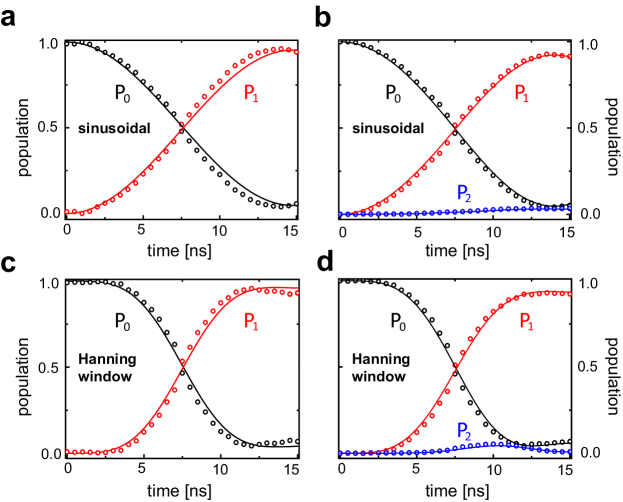
Since the phase qubit arises from a multi-level anharmonic oscillator MartinisReview , a three-level system, $\{|0\rangle,|1\rangle,|2\rangle\}$, is employed to re-examine the state transfer process. The Hamiltonian is changed to $H(t)=(\hbar/2)\bm{B}(t)\cdot\bm{S}+\hbar\Delta_{2}|2\rangle\langle 2|$. The vector $\bm{S}=(S_{x},S_{y},S_{z})$ is defined as $S_{x}=\sum_{n=0}^{1}\sqrt{n+1}(|n+1\rangle\langle n|+h.c.)$, $S_{y}=\sum_{n=0}^{1}\sqrt{n+1}(i|n+1\rangle\langle n|+h.c.)$, and $S_{z}=\sum_{n=0}^{2}(1-2n)|n\rangle\langle n|$. A large anharmonic frequency shift, $\Delta_{2}/2\pi=-200$ MHz, exists in our system. By experimentally projecting onto the three quantum states, the corrected population evolutions are plotted in Fig. 1b. A small but nonzero population $P_{2}(t)$ of the second excited state is increased with time, causing a population leakage out of $\{|0\rangle,|1\rangle\}$. The actual populations transferred in the STA operation are $P_{1}(t=T_{a})=0.907$ and $P_{2}(t=T_{a})=0.036$. The necessarity of the three-level system is also confirmed by good agreement between the Lindblad calculation and the experimental measurement.

The final population at the second excited state is approximated as $P_{2}(t=T_{a})\approx\dot{\theta}(t=T_{a})^{2}/[2(\Delta_{2}+\Omega)^{2}]$ (see Methods). To reduce its influence, we apply an constraint of $\dot{\theta}(t=T_{a})=0$ to re-design the polar angle in a Hanning-window form, i.e., $\theta(t)=(\pi/2)[1-\cos(\pi t/T_{a})]$. The counter-diabatic field, $\bm{B}_{\rm cd}(t)=(0,\dot{\theta}(t),0)$, is modified accordingly. The experimental population evolutions subject to the new STA field $\bm{B}(t)$ are plotted in Fig. 1c,d in the frameworks of the two-level and three-level systems, respectively. The population at the first excited state is increased to $P_{1}(t=T_{a})=0.923$ while the population at the second excited state is decreased to $P_{2}(t=T_{a})=0.009$. Due to a more efficient control on the population leakage, the Hanning-window pulse rather than the simpler sinusoidal pulse will be under investigation in the rest of this paper.

Derivative removal by adiabatic gates. To visualize the trajectory of the entire state transfer process, the quantum state tomography (QST) is performed every 0.5 ns to extract the density matrix $\rho(t)$ LuceroNatPhys12 . For convenience, the QST measurement is restricted to the qubit subspace, $\{|0\rangle,|1\rangle\}$. The experimental Bloch vector, $\bm{r}(t)=(\langle x(t)\rangle,\langle y(t)\rangle,\langle z(t)\rangle)$, is determined by the three projections, $\langle\zeta(t)\rangle=\mathrm{Tr}\{\rho(t)\sigma_{\zeta}\}$ with $\zeta=x,y,z$. The trajectory of $\bm{r}(t)$ is depicted on the Bloch sphere in Fig. 2a, while the time evolutions of the three projections are plotted in Fig. 2b-d respectively. Compared to the ideal trajectory, $\bm{r}(t)=(\cos\theta(t),0,\sin\theta(t))$, the experimental qubit vector gradually shrinks inside the Bloch sphere due to the qubit dissipation. A severer distortion is observed in the $x$-$y$ plane, where both $\langle x(t)\rangle$ and $\langle y(t)\rangle$ deviate from the ideal path (black crosses versus green lines in Fig. 2b,c). This phase error in the $x$-$y$ plane arises mainly from the interaction with the second excited state instead of the qubit dissipation Lucero10 .

Figure 2: (a) The trajectories of the qubit vector depicted on the Bloch sphere. The time evolutions of the three projections: (b) $\langle x(t)\rangle$, (c) $\langle y(t)\rangle$ and (d) $\langle z(t)\rangle$. In a-d, black crosses denote the experimental result without the DRAG correction and under the $\mathcal{R}$-frame, red circles denote the experimental result with the DRAG correction and under the $\mathcal{D}$-frame, and the green lines denote the theoretical prediction of an ideal adiabatic state transfer.

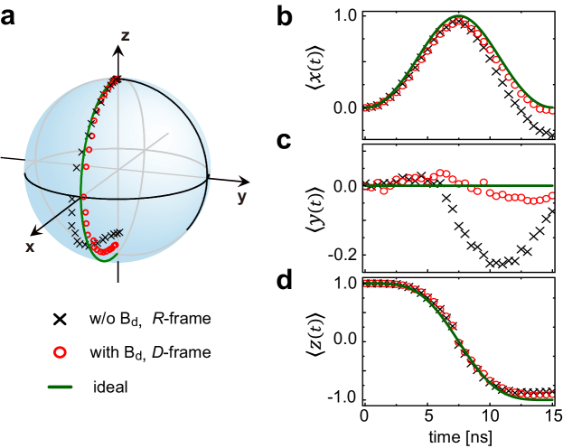
The DRAG method has been theoretically proposed to remove the influence of higher excited states MotzoiPRL09 ; GambettaPRA11 . As described in Methods, an extra pulse $\bm{B}_{\mathrm{d}}(t)$ is supplemented to the STA pulse $\bm{B}(t)$, leading to the modified field as $\bm{B}^{\prime}(t)=\bm{B}(t)+\bm{B}_{\mathrm{d}}(t)$. Under a specified rotating frame characterized by its reference time propagator $\mathcal{D}(t)$, the transformed Hamiltonian is factorized as $H_{\mathcal{D}}(t)=\left[\varepsilon(t)I_{2}+(\hbar/2)\bm{B}(t)\cdot\bm{\sigma}\right]\oplus\varepsilon_{2}(t)|2\rangle\langle 2|$, where $I_{2}=|0\rangle\langle 0|+|1\rangle\langle 1|$ is an identity operator, and $\varepsilon(t)$ and $\varepsilon_{2}(t)$ are two shifted energies MotzoiPRL09 ; GambettaPRA11 . The qubit subspace of $\{|0\rangle,|1\rangle\}$ becomes isolated with the second excited state $|2\rangle$. The quantum operations of the two-level qubit are accomplished under the $\mathcal{D}$-frame. The forms of $\bm{B}_{\mathrm{d}}(t)$ and $\mathcal{D}(t)$ are difficult to be solved exactly. Here we take an approximate DRAG correction GambettaPRA11 . By assuming a zero correction along $z$-direction, the DRAG field is analytically written as $\bm{B}_{\mathrm{d}}(t)=(B_{\mathrm{d};x}(t),B_{\mathrm{d};y}(t),0)$ with $B_{\mathrm{d};x}(t)=(1/4\Delta_{2})[2\ddot{\theta}(t)-\Omega^{2}\sin 2\theta(t)]$ and $B_{\mathrm{d};y}(t)=-(\Omega/\Delta_{2})\dot{\theta}(t)\cos\theta(t)$. The detailed $3\times 3$ matrix form of $\mathcal{D}(t)$ is provided in Supplementary Information.

Next we perform the QST to measure the experimental trajectory subject to the external field $\bm{B}^{\prime}(t)$ after the DRAG correction. The density matrix under the $\mathcal{D}$-frame, $\rho_{\mathcal{D}}(t)=\mathcal{D}^{+}(t)\rho(t)\mathcal{D}(t)$, is calculated using the counterpart $\rho(t)$ under the $\mathcal{R}$-frame. For the $3\times 3$ density matrix $\rho(t)$, an approximation, $\rho_{n2}(t)=\rho_{2n}(t)=\sqrt{P_{n}(t)P_{2}(t)}$ with $n=0,1$, is applied which is acceptable due to a large anharmonicity parameter $\Delta_{2}$ and a small value of $P_{2}(t)$. The trajectory, $\bm{r}_{\mathcal{D}}(t)=\mathrm{Tr}\{\rho_{\mathcal{D}}(t)\bm{\sigma}\}$, calculated under the $\mathcal{D}$-frame is depicted in Fig. 2a, while the projections $\langle\zeta_{\mathcal{D}}(t)\rangle$ along the three directions ($\zeta=x,y,z$) are plotted in Fig. 2b-d respectively. Compared to the result without the DRAG correction, the phase error in the $x$-$y$ plane is significantly suppressed. The $x$-projection $\langle x_{\mathcal{D}}(t)\rangle$ agrees very well with the ideal result and the maximum error of $\langle y_{\mathcal{D}}(t)\rangle$ becomes less than 0.05. The final populations at the two excited states are further improved to $P_{1}(T_{a})=0.95$ and $P_{2}(T_{a})=0.004$. A fast adiabatic trajectory is thus reliably achieved in our phase qubit with the assistance of the STA protocol and the DRAG correction.

Simulating the topological transition by real-time fast adiabatic trajectories. For the SSH model, each unit cell consists of two inequivalent sites ($A$ and $B$, see Supplementary Material). The single-spinless-electron Hamiltonian reads

$$H=(\hbar\Omega_{1}/2)\sum_{n}\left(|n,A\rangle\langle n,B|+h.c.\right)+(\hbar\Omega_{2}/2)\sum_{n}\left(|n,B\rangle\langle n+1,A|+h.c.\right),$$ (1)

where $|n,A\rangle$ ($|n,B\rangle$) is the electronic wavefunction of site $A$ ($B$) in the $n$-th unit cell, and $\Omega_{1}$ ($\Omega_{2}$) is twice the intracell (intercell) hopping amplitude in the unit of angular frequency Asboth2016short . With a periodic boundary condition, the bulk Hamiltonian in Eq. (1) is block diagonalized in a quasi-momentum space, i.e., $H=\sum_{\theta}H(\theta)$. The block element at each quasi-momentum $\theta$ is given by $H(\theta)=(\hbar/2)\bm{B}_{0}(\theta)\cdot\bm{\sigma}$ with $\bm{B}_{0}(\theta)=(\Omega_{1}+\Omega_{2}\cos\theta,\Omega_{2}\sin\theta,0)$ and $0\leq\theta\leq 2\pi$. To be consistent with the above adiabatic state transfer, the external field is rotated to be $\bm{B}_{0}(t)=(\Omega_{2}\sin\theta(t),0,\Omega_{1}+\Omega_{2}\cos\theta(t))$. The time evolution of $\theta(t)$ mimics a pathway of the quasi-momentum traversing the FBZ.

Figure 3: The trajectories of the qubit vector $\bm{r}_{\mathcal{D}}(\theta)|_{\theta=\theta(t)}$ on the Bloch sphere. (a) With the hopping amplitude ratio $\alpha=\Omega_{1}/\Omega_{2}=0$. (b) With $\alpha=1.2$. (c) The polar angle $\theta_{\rm q}$ of the Bloch eigenstate versus the quasi-momentum $\theta$. From top to bottom, symbols are experimental results of $\alpha=0$ (black circles), $\alpha=0.6$ (red up-triangles), $\alpha=1$ (blue down-triangles), $\alpha=1.2$ (green diamonds) and $\alpha=1.6$ (purple pluses). The solid lines are the theoretical predictions under the ideal conditions. (d) The topological invariants as the functions of $\alpha$. The red circles and blue up-triangles denote the experimental result of the winding number for the 1D SSH model and the Chern number for a toy 2D model, respectively. The green solid line is the theoretical prediction of the ideal topological transitions in these two systems.

In our experiment, the intercell hopping amplitude is fixed at $\Omega_{2}/2\pi=30$ MHz while the intracell hopping amplitude $\Omega_{1}$ is varied to simulate the topological transition. The phase qubit is initially reset at the ground state. The Hanning-window form, $\theta(t)=(\pi/2)[1-\cos(\pi t/T_{a})]$, is chosen for the time evolution of the quasi-momentum. Due to the intrinsic symmetry of the Hamiltonian, the operation is limited to a half-circle transition with $0\leq\theta(t)\leq\pi$. The STA protocol with the counter-diabatic field $\bm{B}_{\mathrm{cd}}(t)$ is applied for a fast adiabatic manipulation, in which the operation time is set as $T_{a}=20$ ns. The DRAG field $\bm{B}_{\mathrm{d}}(t)$ is also included to suppress the influence of highly excited states. The QST measurement is performed every 0.5 ns so that the total $M=41$ quasi-momenta are probed. The measured density matrix is subsequently transformed into $\rho_{\mathcal{D}}(t)=\mathcal{D}^{+}(t)\rho(t)\mathcal{D}(t)$ under the $\mathcal{D}$-frame.

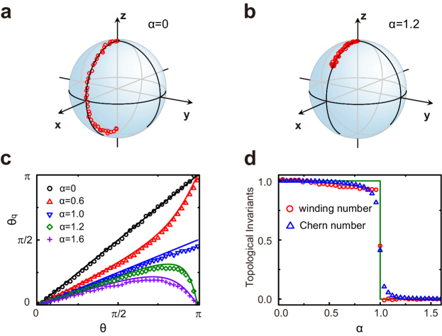
For the SSH model, the dispersion relation of the two bulk Bloch bands is unchanged if the values of $\Omega_{1}$ and $\Omega_{2}$ are swapped. However, the topology of the SSH model is sensitive to the ratio of the two hopping amplitudes, $\alpha=\Omega_{1}/\Omega_{2}$. In the case of $\alpha>1$, the SSH model behaves as a conventional insulator. In the opposite case of $\alpha<1$, two eigenstates with almost-zero eigenenergies appear at the two ends of the SSH model (see Supplementary Information). Following the bulk-boundary correspondence, the emergence of the edge states can be understood alternatively from the change of the bulk Bloch eigenstates. As an illustration, we present the experimental evolutions at two typical ratios, $\alpha=0$ and $\alpha=1.2$. The trajectories of the qubit vector, $\bm{r}_{\mathcal{D}}(t)=\mathrm{Tr}\{\rho_{\mathcal{D}}(t)\bm{\sigma}\}$, are depicted in Fig. 3a,b respectively. As the quasi-momentum evolves from 0 to $\pi$, the qubit vector evolves from the north to south pole for $\alpha=0$ while the qubit vector is retracted to the initial north pole for $\alpha=1.2$. The separation of the two topological phases are visualized by the different trajectories of $\bm{r}_{\mathcal{D}}(t)$.

The polar angle, $\theta_{\rm q}(\theta)=\arccos\left[\langle z_{\mathcal{D}}(t)\rangle/\sqrt{\langle x_{\mathcal{D}}(t)\rangle^{2}+\langle z_{\mathcal{D}}(t)\rangle^{2}}\right]$, is experimentally determined to characterize the bulk Bloch eigenstate $|u(\theta)\rangle$. The $y$-projection $\langle y_{\mathcal{D}}(t)\rangle$ is discarded to reduce the phase error in the estimation. In Fig. 3c, we present the results of $\theta_{\rm q}(\theta)$ for the five hopping amplitude ratios. Under each condition, the experimental measurement agrees quantitatively well with the theoretical prediction, $\theta_{\rm q}(\theta)=\arccos\left[(\alpha+\cos\theta)/\sqrt{1+\alpha^{2}+2\alpha\cos\theta}\right]$. For $\alpha=0$ and $\alpha=0.6$, the two polar angles monotonically increase with $\theta$ and reach the almost same value, $\theta_{\rm q}(\theta=\pi)\approx\pi$, at the end of the trajectory. For $\alpha=1.2$ and $\alpha=1.6$, the two polar angles decrease to zero after an initial increase. The linear line, $\theta_{\rm q}(\theta)\approx\theta/2$ at $\alpha=1$, represents the transition behavior separating the two topological phases. For the other half of the FBZ ($\pi\leq\theta\leq 2\pi$), the dependence of $\theta_{\rm q}(\theta)$ on the quasi-momentum $\theta$ can be deduced using a symmetry argument. The periodic condition of the bulk Bloch eigenstate, $|u(\theta+2\pi)\rangle=|u(\theta)\rangle$, requires $\theta_{\rm q}(\theta+2\pi)=\theta_{\rm q}(\theta)+2\nu\pi$ with $\nu$ an integer. In the SSH model, this integer is given by $\nu=0$ for $\alpha>1$ and $\nu=1$ for $\alpha<1$. The topological invariant $\nu$ is equivalent to the winding number of the curve $\bm{r}_{\mathcal{D}}(\theta)$ circulating around the center of the Bloch sphere. Under the ideal condition, the winding number is defined as

$$\nu=\frac{1}{2\pi}\int_{0}^{2\pi}\bm{e}_{y}\cdot\left[\tilde{\bm{B}}_{0}(\theta)\times d_{\theta}\tilde{\bm{B}}_{0}(\theta)\right]d\theta,$$ (2)

where $\tilde{\bm{B}}_{0}(\theta)=\bm{B}_{0}(\theta)/|\bm{B}_{0}(\theta)|$ is a normalized vector and $\bm{e}_{y}$ is the unit vector along the $y$-direction Asboth2016short . Experimentally, this number is estimated using $\nu=(1/\pi)[\theta_{\rm q}(\theta=\pi)-\theta_{\rm q}(\theta=0)]$. As shown in Fig. 3d, a sharp topological transition of the SSH model is identified by our experimental measurement of $\nu$, which is very close to the theoretical prediction.

Similar to two earlier studies RoushanNat14 ; SchroerPRL14 , the external field can be extended to be $\bm{B}_{0}(\theta,\phi)=(\Omega_{2}\sin\theta\cos\phi,\Omega_{2}\sin\theta\sin\phi,\Omega_{1}+\Omega_{2}\cos\theta)$, where the vector of $(\theta,\phi)$ defines a 2D quasi-momentum. To cover the entire 2D FBZ of the spherical surface, we can perform the adiabatic state transfer driven by $\bm{B}_{0}(\theta(t),\phi(t)=\phi)$ and then the constant azimuthal angle $\phi$ is increased by small steps to form a closed circle of $0\leq\phi\leq 2\pi$. The Chern number,

$$\mathcal{C}h=\frac{1}{4\pi}\int\int\tilde{\bm{B}}_{0}(\theta,\phi)\cdot\left[\partial_{\theta}\tilde{\bm{B}}_{0}(\theta,\phi)\times\partial_{\phi}\tilde{\bm{B}}_{0}(\theta,\phi)\right]d\theta d\phi,$$ (3)

is the topological invariant of 2D systems HasanRMP10 . For our given FBZ, Eq. 3 is simplified to be $\mathcal{C}h=(1/2)\int_{0}^{\pi}\sin\theta_{\rm q}(\theta)(\partial_{\theta}\theta_{\rm q})d\theta$, which can thus be simulated by the adiabatic trajectory subject to the 1D control parameter $\theta(t)$. In our experiment, we use the data in Fig. 3c to estimate the Chern number using a summation, $\mathcal{C}h=(1/2)\sum_{m=0}^{M-1}[\theta_{\rm q}(m+1)-\theta_{\rm q}(m)]\sin[(\theta_{\rm q}(m+1)+\theta_{\rm q}(m))/2]$. Figure 3d demonstrates a quantitative agreement between the experimental measurement and the theoretical prediction: $\mathcal{C}h=1$ for $\alpha<1$ and $\mathcal{C}h=0$ for $\alpha>1$. The fast adiabatic trajectories obtained in our 1D experiment thus simulate the topological transition in a simple 2D model.

Figure 4: The trajectories of the qubit vector $\bm{r}_{\mathcal{D}}(\theta)|_{\theta=\theta_{m}(t=T_{a})}$ on the Bloch sphere. (a) With $\alpha=0$. (b) With $\alpha=1.2$. (c) The polar angle $\theta_{\rm q}$ of the bulk Bloch eigenstate versus the quasi-momentum $\theta$. The parameters are the same as those in Fig. 3c. (d) The topological invariants as the functions of $\alpha$. In a-d, all the symbols and lines are defined in the same way as their counterparts in Fig. 3.

Simulating the topological transition by virtual fast adiabatic trajectories. For an ideal adiabatic process, each segment can be regarded as an independent adiabatic process. A complete adiabatic trajectory is alternatively achieved by a series of adiabatic state transfers when the control parameter is terminated at intermediate positions along its designed pathway. Following this simulation scheme, the time evolution of the control parameter is changed to be $\theta_{m}(t)=(\pi/2m)[1-\cos(\pi t/T_{a})]$, which mimics an even distribution of the quasi-momentum by $\theta_{m}(t=T_{a})=\pi/m$. The total $M=41$ ($0\leq m\leq M$) external fields, $\bm{B}_{0}(t)=(\Omega_{2}\sin\theta_{m}(t),0,\Omega_{1}+\Omega_{2}\cos\theta_{m}(t))$, are applied to generate a virtual adiabatic trajectory in our experiment. For each $m$-th field, both counter-diabatic and DRAG fields, $\bm{B}_{\mathrm{cd}}(t)$ and $\bm{B}_{\mathrm{d}}(t)$, are supplemented for a fast adiabatic state transfer. The QST measurement is performed only at the end of the STA operation with $T_{a}=20$ ns. In Fig. 4, we present in detail the experimental results based on the virtual trajectories of $\bm{r}_{\mathcal{D}}(\theta)|_{\theta=\theta_{m}(t=T_{a})}$. All the figures are drawn in the same way as their counterparts in Fig. 3 based on the real-time trajectories of $\bm{r}_{\mathcal{D}}(\theta)|_{\theta=\theta(t)}$. By comparing the results in Fig. 3 and Fig. 4, we find that the accuracies of these two simulation methodologies are close to each other. Therefore, the virtual adiabatic trajectories provide an alternative method to reliably simulating the topological transition.

Discussion and conclusion
The quantum simulation in this article is built on the technique of fast adiabatic state transfers. The underlined STA protocol and its extensions have been shown to maintain adiabaticity in a fast operation, which can help establish practical applications of adiabatic procedures. As our experiment is focused on a single qubit, it will be worth exploring in the future the STA protocol in multi-qubit systems. The multi-level effect is common in many practical quantum systems. The DRAG correction applied in our experiment is an efficient way to exclude the influence of highly excited states. The implementation of the STA protocol and the DRAG correction often requires a complicated drive pulse, which can however be reliably generated in a superconducting qubit system with a sophisticated microwave control technique.

In perivous studies of simulating the topological transition, the experiments were performed by measuring local non-adiabatic responses, integrated phases and transport quantities. Alternatively, the fast adiabatic evolution of the spin-up state in our experiment is a simple but transparent method of visualizing the bulk Bloch eigenstates which include all the geometric and topological information. The sharp transitions in our measurements of the winding number and the Chern number verify a strong protection of topological phases unless the energy gap is closed and reopened around the transition point. The virtual construction of the adiabatic trajectory in addition to the real-time approach provides the flexibility in mimicking the FBZ. Although a 1D quasi-momentum is considered in our study, this simulation method can be straightforwardly extended to a realistic 2D system. After collecting multiple adiabatic trajectories, we may obtain the Bloch eigenstates over the entire 2D FBZ, which will be explored in the future.

Methods
Experimental setup. The superconducting phase qubit used in this experiment is the same as that in our previous experiment ZZXPRA17 . An anharmonic LC resonator is formed by an Al/AlOx/Al Josephson junction coupled with a parallel capacitor ($C_{\mathrm{q}}=1$ pF) and a loop inductor ($L_{\mathrm{q}}=720$ pH). The lowest two energy levels ($\varepsilon_{0}$ and $\varepsilon_{1}$) are used as the ground and excited states of a qubit, and their resonance frequency is $\omega_{10}=(\varepsilon_{1}-\varepsilon_{0})/\hbar$. The second excited state with energy $\varepsilon_{2}$ induces an ahhamonic frequency shift, $\Delta_{2}=\omega_{21}-\omega_{10}=(\varepsilon_{2}+\varepsilon_{0}-2\varepsilon_{1})/\hbar$. In our experiment, these two parameters are given by $\omega_{10}/{2\pi}=5.7$ GHz and $\Delta_{2}/{2\pi}=-200$ MHz. The microwave drive signal is synthesized by an IQ mixer in which two low-frequency quadratures are mixed with a local oscillator signal. A on-chip superconducting quantum interference device (SQUID) is used to measure the population of various qubit states (see Supplementary Information). The density matrix is further extracted by the QST method.

Counter-diabatic field in the STA protocol. A non-degenerate reference Hamiltonian $H_{0}(t)$ is diagonalized in the instantaneous eigen basis set, leading to $H_{0}(t)=\sum_{n}\varepsilon_{n}(t)|n(t)\rangle\langle n(t)|$ where $|n(t)\rangle$ is the $n$-th instantaneous eigenstate and $\varepsilon_{n}(t)$ is its eigenenergy. In a slow adiabatic operation, a quantum system initially at $|n(t=0)\rangle$ can remain at this eigenstate. The system wavefunction is given by $|\psi(t)\rangle=\exp[i\varphi(t)]|n(t)\rangle$, where $\varphi(t)$ is an accumulated phase. The non-adiabatic transitions can however destroy adiabaticity. To speed-up the adiabatic operation while maintaining adiabaticity, the STA protocol requires an additional counter-diabatic Hamiltonian $H_{\mathrm{cd}}(t)$. The wavefunction is expanded as $|\psi(t)\rangle=\sum_{n}a_{n}(t)|n(t)\rangle$. With respect to the total Hamiltonian, $H(t)=H_{0}(t)+H_{\mathrm{cd}}(t)$, the time evolution of each coefficient $a_{n}(t)$ follows

$$\hbar\dot{a}_{n}(t) = -i\left[\varepsilon_{n}(t)-i\hbar\langle n(t)|\partial_{t}n(t)\rangle\right]a_{n}(t)-i\langle n(t)|H_{\mathrm{cd}}(t)|n(t)\rangle a_{n}(t)$$ (4)

$$-i\sum_{m(\not=n)}\left[-i\hbar\langle n(t)|\partial_{t}m(t)\rangle+\langle n(t)|H_{\mathrm{cd}}(t)|m(t)\rangle\right]a_{m}(t).$$

To recover the adiabatic evolution under the reference Hamiltonian, the constraints,

$$\langle n(t)|H_{\mathrm{cd}}(t)|m(t)\rangle=\left\{\begin{array}[]{ll}0&~{}~{}\mathrm{for}~{}~{}~{}m=n\\ i\hbar\langle n(t)|\partial_{t}m(t)\rangle&~{}~{}~{}\mathrm{for}~{}~{}~{}m\neq n\end{array}\right.,$$ (7)

are required for the counter-diabatic Hamiltonian, which is satisfied by

$$H_{\mathrm{cd}}(t)=i\hbar\sum_{n}\big{[}|\partial_{t}n(t)\rangle\langle n(t)|-\langle n(t)|\partial_{t}n(t)\rangle|n(t)\rangle\langle n(t)|\big{]}.$$ (8)

For a spin-half particle, the reference Hamiltonian in general follows $H_{0}(t)=\hbar\bm{B}_{0}(t)\cdot\bm{\sigma}/2$ with $\bm{B}_{0}(t)=|\bm{B}_{0}(t)|(\sin\theta(t)\cos\phi(t),\sin\theta(t)\sin\phi(t),\cos\theta(t))$. The amplitude of this external field, $|\bm{B}_{0}(t)|$, gives rise to the two eigenenergies, $\varepsilon_{\uparrow,\downarrow}(t)=\pm\hbar|\bm{B}_{0}(t)|/2$, while the two angle variables, $\{\theta(t),\phi(t)\}$, determine the two eigenstates,

$$\left\{\begin{array}[]{ccc}|s_{\uparrow}(t)\rangle&=&\cos\left[\frac{\theta(t)}{2}\right]|0\rangle+\sin\left[\frac{\theta(t)}{2}\right]e^{i\phi(t)}|1\rangle\\ |s_{\downarrow}(t)\rangle&=&-\sin\left[\frac{\theta(t)}{2}\right]e^{-i\phi(t)}|0\rangle+\cos\left[\frac{\theta(t)}{2}\right]|1\rangle\end{array}\right..$$ (11)

Next we substitute Eq. 11 into Eq. 8 and obtain the three elements of the counter-diabatic field, which are given by

$$\left\{\begin{array}[]{ccl}B_{\mathrm{cd};x}(t)&=&-\dot{\theta}(t)\sin\phi(t)-\dot{\phi}(t)\sin\theta(t)\cos\theta(t)\cos\phi(t)\\ B_{\mathrm{cd};y}(t)&=&\dot{\theta}(t)\cos\phi(t)-\dot{\phi}(t)\sin\theta(t)\cos\theta(t)\sin\phi(t)\\ B_{\mathrm{cd};z}(t)&=&\dot{\phi}(t)\sin^{2}\theta(t)\end{array}\right..$$ (15)

Equation 15 can be further rewritten in a cross product form as

$$\bm{B}_{\mathrm{cd}}(t)=\frac{1}{|\bm{B}_{0}(t)|^{2}}\bm{B}_{0}(t)\times\dot{\bm{B}}_{0}(t),$$ (16)

which is always orthogonal to the reference field $\bm{B}_{0}(t)$. For the special case of $\bm{B}_{0}(t)=(\Omega\sin\theta(t),0,\Omega\cos\theta(t))$, the counter-diabatic field is written as $\bm{B}_{\mathrm{cd}}(t)=(0,\dot{\theta}(t),0)$.

Population evolution of the second excited state. The anharmonicity in our phase qubit cannot be ignored and the framework of a three-level system is necessary. Under the $\mathcal{R}$-frame, the three-level Hamiltonian of an anharmonic oscillator is given by $H(t)=(\hbar/2)\bm{B}(t)\cdot\bm{S}+\hbar\Delta_{2}|2\rangle\langle 2|$ with the STA field $\bm{B}(t)=\bm{B}_{0}(t)+\bm{B}_{\mathrm{cd}}(t)=(\Omega\sin\theta(t),\dot{\theta}(t),\Omega\cos\theta(t))$. A diagonalization is applied to the qubit subspace, $\{|0\rangle,|1\rangle\}$, giving the instantaneous spin-up ($|s_{\uparrow}(t)\rangle$) and spin-down ($|s_{\downarrow}(t)\rangle$) states subject to the reference field $\bm{B}_{0}(t)$. The time-varying basis set is changed to $\{|s_{\uparrow}(t)\rangle,|s_{\downarrow}(t)\rangle,|2\rangle\}$, and the Hamiltonian is transformed accordingly. If the qubit is designed to follow the adiabatic trajectory of the spin-up state, we can focus on the subspace of $\{|s_{\uparrow}(t)\rangle,|2\rangle\}$ and omit $|s_{\downarrow}(t)\rangle$. The partial Hamiltonian governing the state evolution within this subspace is given by

$$H(t)=(\hbar\Omega/2)|s_{\uparrow}(t)\rangle\langle s_{\uparrow}(t)|+\hbar\Delta^{\prime}_{2}(t)|2\rangle\langle 2|+\hbar\left[J_{\uparrow 2}(t)|s_{\uparrow}(t)\rangle\langle 2|+h.c.\right],$$ (17)

with $\Delta^{\prime}_{2}(t)=\Delta_{2}-(3/2)\Omega\cos\theta(t)$ and $J_{\uparrow 2}(t)=(\sqrt{2}/2)\sin[\theta(t)/2]\left[\Omega\sin\theta(t)-i\dot{\theta}(t)\right]$. Next we assume an adiabatic evolution beginning with the initial state $|s_{\uparrow}(t=0)\rangle=|0\rangle$. The population of the second excited state is then approximated as

$$P_{2}(t) \approx \frac{1}{2}\left[1-\frac{|\Delta^{\prime}_{2}(t)-\Omega/2|}{\sqrt{[\Delta^{\prime}_{2}(t)-\Omega/2]^{2}+4|J_{\uparrow 2}(t)|^{2}}}\right]$$ (18)

$$\approx \frac{|J_{\uparrow 2}(t)|^{2}}{[\Delta^{\prime}_{2}(t)-\Omega/2]^{2}},$$

where the second equation is obtained under the consideration of $|\Delta_{2}|\gg\Omega,|\dot{\theta}(t)|$. For a polar angle with $\theta(t=T_{a})=\pi$, the final population of the second excited state becomes $P_{2}(t=T_{a})\approx\dot{\theta}(t=T_{a})^{2}/[2(\Delta_{2}+\Omega)^{2}]$ .

First-order approximation of the DRAG correction. For a multi-level anharmonic oscillator, the DRAG method is proposed to isolate the qubit subspace $\{|0\rangle,|1\rangle\}$ from higher excited states (detailed in Supplementary Information). In the case of the three-level system, the above STA Hamiltonian is expanded over a perturbation parameter $\Delta^{-1}_{2}$, giving $H(t)=H^{(-1)}(t)+H^{(0)}(t)$ with $H^{(-1)}(t)=\hbar\Delta_{2}|2\rangle\langle 2|$ and $H^{(0)}(t)=(\hbar/2)\bm{B}(t)\cdot\bm{S}$. The DRAG field $\bm{B}_{\rm d}(t)$ is responsible for higher order corrections, $H_{\rm d}(t)=H^{(1)}(t)+\cdots=(\hbar/2)[\bm{B}^{(1)}_{\rm d}(t)+\cdots]\cdot\bm{S}$. The modified total Hamiltonian is written as $H^{\prime}(t)=H(t)+H_{\rm d}(t)$. The time evolution of this three-level system is inspected under an alternative $\mathcal{D}$-frame, which is defined by its reference time propagator, $\mathcal{D}(t)=\exp[-i\mathcal{M}(t)]$. The same expansion over $\Delta^{-1}_{2}$ is applied to the exponent term $\mathcal{M}(t)$, giving $\mathcal{M}(t)=\mathcal{M}^{(1)}(t)+\mathcal{M}^{(2)}(t)+\cdots$. The transformation from the original $\mathcal{R}$-frame to the new $\mathcal{D}$-frame changes the total Hamiltonian to be

$$H_{\mathcal{D}}(t)=\mathcal{D}^{+}(t)H^{\prime}(t)\mathcal{D}(t)+i\dot{\mathcal{D}}^{+}(t)\mathcal{D}(t),$$ (19)

and the density matrix follows $\rho_{\mathcal{D}}(t)=\mathcal{D}^{+}(t)\rho(t)\mathcal{D}(t)$.

Under the construction of the DRAG method, we expect a factorized form, $H_{\mathcal{D}}(t)=[\varepsilon(t)I_{2}+(\hbar/2)\bm{B}(t)\cdot\bm{\sigma}]\oplus\varepsilon_{2}(t)|2\rangle\langle 2|$, for the transformed Hamiltonian. The two energies also follow the expansion over $\Delta^{-1}_{2}$, giving $\varepsilon(t)=\varepsilon^{(1)}(t)+\cdots$ and $\varepsilon_{2}(t)=\hbar\Delta_{2}+\varepsilon^{(0)}_{2}(t)+\varepsilon^{(1)}_{2}(t)+\cdots$. Two additional constraints, $\mathcal{D}(t=0)=1$ and $\mathcal{D}(t=T_{a})=1$, are considered so that the $\mathcal{D}$-frame recovers the $\mathcal{R}$-frame at the initial and final moments of the operation. Next we expand both sides of Eq. 19 over $\Delta^{-1}_{2}$ order by order, which results in a series of equations for $\{\bm{B}^{(i)}_{\rm d}(t)\}$ and $\{\mathcal{M}^{(i)}(t)\}$. These equations are however difficult to be solved exactly. In our experiment, we truncate the expansion of Eq. 19 up to the first order of $\Delta^{-1}_{2}$. Consequently, we obtain $\bm{B}_{\rm d}(t)\approx\bm{B}^{(1)}_{\rm d}(t)$ and $\mathcal{D}(t)\approx\exp\{-i[\mathcal{M}^{(1)}(t)+\mathcal{M}^{(2)}(t)]\}$ while the explicit forms of the three perturbations are provided in Supplementary Information.

Acknowledgements
The work reported here is supported by the National Basic Research Program of China (2014CB921203, 2015CB921004), the National Natural Science Foundation of China (NSFC-11374260, NSFC-21173185), and the Fundamental Research Funds for the Central Universities in China (2016XZZX002-01). Devices were made at John Martinis’s group using equipments of UC Santa Barbara Nanofabrication Facility, a part of the NSF-funded National Nanotechnology Infrastructure Network.

Conflicts of interest
The authors declare that they have no competing interests.

References

- (1) Klitzing KV, Dorda G, Pepper M (1980) New method for high-accuracy determination of the fine-structure constant based on quantized hall resistance. Phys Rev Lett 45:494-497
- (2) Thouless D, Kohmoto M, Nightingale M, Den Nijs M (1982) Quantized hall conductance in a two-dimensional periodic potential. Phys Rev Lett 49:405-408
- (3) Su WP, Schrieffer JR, Heeger AJ (1979) Solitons in polyacetylene. Phys Rev Lett 42:1698-1701
- (4) Asbóth JK, Oroszlány, L, Pályi A (2016) A short course on topological insulators. Lecture Notes in Physics (Springer International Publishing)
- (5) Kitagawa T et al (2011) Observation of topologically protected bound states in photonic quantum walks. Nat Commun 3:882
- (6) Atala M et al (2013) Direct measurement of the zak phase in topological bloch bands. Nat Phys 9:795-800
- (7) Jotzu G et al (2014) Experimental realization of the topological haldane model with ultracold fermions. Nature 515:237-240
- (8) Aidelsburger M et al (2015) Measuring the chern number of hofstadter bands with ultracold bosonic atoms. Nat Phys 11:162-166
- (9) Duca L et al (2015) An aharonov-bohm interferometer for determining bloch band topology. Science 347:288-292
- (10) Mittal S, Ganeshan S, Fan J, Vaezi A, Hafezi M (2016) Measurement of topological invariants in a 2d photonic system. Nat Photon 10:180-183
- (11) Fläschner N et al (2016) Experimental reconstruction of the Berry curvature in a Floquet Bloch band. Science 352:1092-1094
- (12) Goldman N, Budich JC, Zoller P (2016) Topological quantum matter with ultracold gases in optical lattices. Nat Phys 12:639-645
- (13) Roushan P et al (2014) Observation of topological transitions in interacting quantum circuits. Nature 515:241-244
- (14) Schroer M et al (2014) Measuring a topological transition in an artificial spin-1/2 system. Phys Rev Lett 113:050402
- (15) Flurin E et al (2016) Observing topological invariants using quantum walk in superconducting circuits. Phys Rev X 7:031023
- (16) Kong, Fei et al (2016) Direct measurement of topological numbers with spins in diamond. Phys Rev Lett 117:060503
- (17) Hasan MZ, Kane CL (2010) Colloquium: topological insulators. Rev Mod Phys 82:3045-3067
- (18) Farhi E, Goldstone J, Gutmann S, Sipser M (2000) Quantum computation by adiabatic evolution.. Preprint at https://arxiv.org/abs/quant-ph/0001106
- (19) Nielsen MA, Chuang IL (2000) Quantum computation and quantum information. Cambridge Univ Press Canbridge
- (20) Demirplak M, Rice SA (2003) Adiabatic population transfer with control fields. J Phys Chem A 107:9937-9945
- (21) Berry M (2009) Transitionless quantum driving. J Phys A 42:365303
- (22) Chen X, Lizuain I, Ruschhaupt A, Guéry-Odelin D, Muga J (2010) Shortcut to adiabatic passage in two-and three-level atoms. Phys Rev Lett 105:123003
- (23) Masuda S, Nakamura K (2009) Fast-forward of adiabatic dynamics in quantum mechanics. Proc R Soc A 466:1135-1154
- (24) Torrontegui E et al (2013) Shortcuts to adiabaticity. Adv At Mol Opt Phys 62:117-169
- (25) Torosov BT, Guérin S, Vitanov NV (2011) High-fidelity adiabatic passage by composite sequences of chirped pulses. Phys Rev Lett 106:233001
- (26) Martinis JM, Geller MR (2014) Fast adiabatic qubit gates using only control. Phys Rev A 90:022307
- (27) Bason MG et al (2012) High-fidelity quantum driving. Nat Phys 8:147-152
- (28) Zhang J et al (2013) Experimental implementation of assisted quantum adiabatic passage in a single spin. Phys Rev Lett 110:240501
- (29) Zhou BB et al (2017) Accelerated quantum control using superadiabatic dynamics in a solid-state lambda system. Nat Phys 13:330-334
- (30) An SM et al (2016) Shortcuts to adiabaticity by counterdiabatic driving for trapped-ion displacement in phase space. Nat Commun 7:12999
- (31) Zhang ZX et al (2017) Measuring the Berry phase in a superconducting phase qubit by a ‘shortcut to adiabaticity’. Phys Rev A 95:042345
- (32) Motzoi F, Gambetta JM, Rebentrost P, Wilhelm FK (2009) Simple pulses for elimination of leakage in weakly nonlinear qubits. Phys Rev Lett 103:110501
- (33) Gambetta JM, Motzoi F, Merkel ST, Wilhelm FK (2011) Analytic control methods for high-fidelity unitary operations in a weakly nonlinear oscillator. Phys Rev A 83:012308
- (34) Lucero E et al (2010) Reduced phase error through optimized control of a superconducting qubit. Phys Rev A 82:042339
- (35) Lu T (2011) Population inversion by chirped pulses. Phys Rev A 84:033411
- (36) Martinis JM (2009) Superconducting phase qubits Quantum Inf Process 8:81
- (37) Lucero E et al (2012) Computing prime factors with a Josephson phase qubit quantum processor. Nat Phys 8:719-723