Galaxy-Galaxy Weak-Lensing Measurements from SDSS: II. Host Halo properties of galaxy groups
Abstract
As the second paper of a series on studying galaxy-galaxy lensing signals using the Sloan Digital Sky Survey Data Release 7 (SDSS DR7), we present our measurement and modelling of the lensing signals around groups of galaxies. We divide the groups into four halo mass bins, and measure the signals around four different halo-center tracers: brightest central galaxy (BCG), luminosity-weighted center, number-weighted center and X-ray peak position. For X-ray and SDSS DR7 cross identified groups, we further split the groups into low and high X-ray emission subsamples, both of which are assigned with two halo-center tracers, BCGs and X-ray peak positions. The galaxy-galaxy lensing signals show that BCGs, among the four candidates, are the best halo-center tracers. We model the lensing signals using a combination of four contributions: off-centered NFW host halo profile, sub-halo contribution, stellar contribution, and projected 2-halo term. We sample the posterior of 5 parameters i.e., halo mass, concentration, off-centering distance, sub halo mass, and fraction of subhalos via a MCMC package using the galaxy-galaxy lensing signals. After taking into account the sampling effects (e.g. Eddington bias), we found the best fit halo masses obtained from lensing signals are quite consistent with those obtained in the group catalog based on an abundance matching method, except in the lowest mass bin.
Subject headings:
(cosmology:) gravitational lensing; galaxies: clusters: general1. Introduction
Modern galaxy formation theory suggests that dark matter halos form first, which provide gravitational potential for galaxies to form. The mass of dark matter halo is thus a critical quantity to understand galaxy formation and constrain the cosmological parameters. There are many methods that can be used to constrain halo mass in observations. The luminosity of X-ray emission from the Intra Cluster Medium (ICM) due to the thermal bremsstrahlung is scaled with the dark matter halo mass assuming an hydro equilibrium state of the gas (Pratt et al., 2009). The Sunyaev-Zeldovich (Sunyaev & Zeldovich, 1972) effect, i.e. the inverse Compton scattering between the high energy electrons from clusters and the CMB photons, is another indicator of cluster mass (Bleem et al., 2015).
Optically, from large photometric galaxy surveys, clusters are selected and assigned with dark matter halo masses in large sky coverages and large redshift ranges. Based on SDSS, SDSS-C4 (Miller et al., 2005) and RedMaPPer (Rykoff et al., 2014) select clusters using photometric data alone, whereas MaxBCG sample (Koester et al., 2007) adds spectroscopic redshift as extra information in selection criteria. All of those samples use an empirical scaling relation between the effective number of member galaxies (richness) and halo mass, a.k.a richness-mass relation, to assign halo masses to clusters. Such methods are mainly applicable for those very massive clusters and need to be scaled with additional measurements.
Based on spectroscopic redshift surveys, galaxy groups can be extracted from halos of much lower mass either by the traditional Friends-Of-Friends (FOF) method (e.g. Eke et al., 2004), or by sophisticated adaptive halo-based group finder(e.g. Yang et al., 2005, 2007, hereafter Y07), which is more reliable in their membership determination. From the group catalogs, a wide variety of mass estimation methods are developed. Y07 applied a luminosity ranking and stellar mass ranking method to obtain halo mass estimation. For poor systems, Lu et al. (2015) introduced an empirical mass estimation method applying the gap between BCG luminosity and satellites luminosity. Assuming a Gaussian velocity distribution, satellite kinematics (van den Bosch et al., 2004) measure the dynamical mass of galaxy groups. Similarly galaxy infall kinematics (Zu & Weinberg, 2013; Zu et al., 2014, GIK) can also be used to constrain the halo mass.
Weak gravitational lensing signal, though statistical in nature, is considered to be another powerful tool to study the property of dark matter distributions due to the fact that the signal is sensitive to all the intervening mass between the observer and the source. The successful measurement of weak lensing signals require high quality imaging of background galaxies. Many recent surveys like CFHTLens (Heymans et al., 2012), DES (Jarvis et al., 2015), and KIDS (Kuijken et al., 2015; Viola et al., 2015), etc., take weak lensing as one of their key scientific projects. Future large surveys, either ground-based or space-based such as EUCLID (Refregier et al., 2010) and LSST (LSST Science Collaboration et al., 2009) also take weak lensing as one of their key projects. The high quality and deep galaxy images in terms of galaxy number per square arc minutes enables one to measure the second order weak lensing studies, a.k.a cosmic shear (Fu et al., 2008; Kilbinger et al., 2013), which are now constantly used to constrain the cosmological parameters such as and .
Sloan Digital Sky Survey (York et al., 2000) initiates the galaxy-galaxy lensing analysis since Fischer et al. (2000). It is followed by Sheldon et al. (2004), who chose MaxBCG sample as lenses binned by richness. Hirata & Seljak (2003) and Mandelbaum et al. (2005, 2006) not only studied the halo properties of lenses from SDSS main sample, but also analysed sources of systematics caused by PSF, selection effect, noise rectification effect and claimed that the final signal should subtract the signal from random sample. Simet et al. (2016) used redMaPPer as lenses and tested the consistency of the mass-richness relation. These galaxy-galaxy lensing signals provided us another method to measure the halo mass of lens systems in consideration.
To obtain reliable galaxy-galaxy lensing measurements, accurate image processing of source galaxies are essential. Many groups have developed image processing pipelines devoted to improving the accuracy of shape measurements (Kaiser et al., 1995; Bertin & Arnouts, 1996; Maoli et al., 2000; Rhodes et al., 2000; van Waerbeke, 2001; Bernstein & Jarvis, 2002; Bridle et al., 2002; Refregier, 2003; Bacon & Taylor, 2003; Hirata & Seljak, 2003; Heymans et al., 2005; Zhang, 2010, 2011; Bernstein & Armstrong, 2014; Zhang et al., 2015). Among these, Lensfit (Miller et al., 2007, 2013; Kitching et al., 2008) applies a Bayesian based model-fitting approach; BFD (Bayesian Fourier Domain) method (Bernstein & Armstrong, 2014) carries out Bayesian analysis in the Fourier domain, using the distribution of un-lensed galaxy moments as a prior, and the Fourier_Quad method developed by (Zhang, 2010, 2011; Zhang et al., 2015; Zhang, 2016) uses image moments in the Fourier Domain.
Very recently, Luo et al. (2017) developed an image processing pipeline and applied it to the SDSS DR7 imaging data. The galaxy-galaxy lensing signals were measured for lens galaxies that are separated into different luminosity bins and stellar mass bins. As the second paper of a series, here we measure the galaxy-galaxy lensing signals using the group catalogs constructed by Yang et al. (2007). We will measure the galaxy-galaxy lensing signals around groups in different mass bins, as well as for four types of halo-center tracers: brightest central galaxy (BCG), luminosity-weighted center (LwCen), number-weighted center (NwCen) and X-ray peak position. We focus on the estimation of halo properties of the groups in consideration such as their halo masses, concentrations and off-center effects, etc.
The structure of this paper is organized as follows. In section 2, we first present the data set and the main results of galaxy-galaxy lensing signals measured around galaxy groups. We show our modelling and parameter constraints in section 3. We discuss the Eddington bias that the group mass estimation may have in section 4. We summarize our results in section 5. Unless stated otherwise, we adopt a LCDM cosmology with , and .
2. The Galaxy-Galaxy Lensing Signals of Galaxy Groups
2.1. Sources
We use the shape catalog created by Luo et al. (2017) based on SDSS DR7 imaging data. The DR7 imaging data, with u, g, r, i and z band, covers about 8423 square degrees of the LEGACY sky (230 million distinct photometric objects). The total number of objects identified as galaxies is around 150 million. These galaxies are further selected and processed by our image pipeline. The galaxies are selected by OBJC_TYPE=3 from PHOTO pipe (Lupton et al., 2001) and must be brighter than 22 in band model magnitude and brighter than 21.6 in band model magnitude. We also apply Flags such as BINNED1 (detected at ), SATURATED=0 (do not have saturated pixels), EDGE=0 (do not locate at the edge of the CCD), MAYBE_CR=0 (not cosmic rays), MAYBE_EGHOST=0 (not electronic ghost line) and PEAKCENTER=0 (centroiding algorithm works well for this subject). In processing the images, the Point Spread Function (PSF) effect was corrected by combining Bernstein & Jarvis (2002) and Hirata & Seljak (2003) method. After the shape measurement, a size cut by resolution factor () was applied. The final shape catalog for our study contains 41,631,361 galaxies with position, shape, shape error and photoZ information.
2.2. Lenses
The galaxies used in our probe are obtained from the New York University Value-Added Galaxy Catalogue (NYU-VAGC; Blanton et al., 2005), which is based on SDSS DR7 (Abazajian et al., 2009) but with an independent set of significantly improved reductions. From the NYU-VAGC, we select all galaxies in the Main Galaxy Sample with an extinction corrected apparent magnitude brighter than , with redshifts in the range and with a redshift completeness . This gives a sample of galaxies with a sky coverage of 7748 square degrees. For each galaxy, we estimate its stellar mass using the fitting formula of Bell et al. (2003).
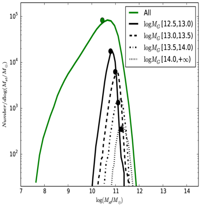
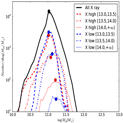
From this galaxy catalog, a total of 472,113 groups are selected using the halo based group finder (Yang et al., 2007), each of which has been assigned with a halo mass by the ranking method. With the halo mass information, we bin the groups with mass into four mass bins. Shown in the left panel of Fig.1 are the stellar mass distribution of all the galaxies (green solid line) and BCGs in different halo mass bins as indicated. The related average values of these galaxies are shown as the solid dots on top of the lines. There is a monotonic increase of average stellar mass of BCGs for the 4 mass bin groups. Tab. 1 lists some properties of the groups in these four mass bins. For each mass bin, we define four types of halo center tracers i.e. BCG, luminosity weighted center (LwCen), number weighted center (NwCen) and X-ray peak position (no X-ray measurement for the first mass bin).
| Sample | |||||
|---|---|---|---|---|---|
| M1 | 101042 | 0.13 | 10.77 | 12.72 | |
| M2 | 43896 | 0.15 | 10.97 | 13.21 | |
| M3 | 14707 | 0.15 | 11.10 | 13.70 | |
| M4 | 4033 | 0.15 | 11.25 | 14.25 |
| Mass bin | |||||
|---|---|---|---|---|---|
| 13.0-13.5 | high | 14582 | 0.14 | 10.97 | 13.24 |
| low | 22086 | 0.15 | 11.00 | 13.23 | |
| 13.5-14.0 | high | 7285 | 0.14 | 11.05 | 13.71 |
| low | 7049 | 0.16 | 11.12 | 13.68 | |
| 14.0-above | high | 2953 | 0.15 | 11.20 | 14.27 |
| low | 1080 | 0.16 | 11.23 | 14.18 |
For the three of our halo bins with halo mass , Wang et al. (2014) measured their X-ray luminosities using the ROSAT data. We divide groups in each of the mass bin into high X-ray luminosity and low X-ray luminosity subsamples with roughly equal numbers using the parameter provided in Wang et al. (2014) catalog, where is the X-ray luminosity of a group in 0.2-2.4kev in unit of erg/s. The related information of these subsamples are listed in Tab. 2. There is a slight difference between the mean redshift of the low X-ray luminosity and high X-ray luminosity subsamples. Both high and low X-ray luminosity samples are assigned with BCG and X-ray peak position as different halo center tracers. Note that since we are using the group masses estimated using the ranking of characteristic group luminosity, while the ones provide in Wang et al. (2014) are based on the ranking of characteristic group stellar mass, some of our groups are not assigned with X-ray luminosities. Thus the total number of groups used in the X-ray high and low subsamples is slightly reduced, especially in the low mass bin.
Shown in the right panel of Fig. 1 are the stellar mass distributions of central galaxies associated with the X-ray peak positions in different halo mass bins as indicated. The dots on top of the lines are their average values. Here results are shown for low X-ray luminosity (blue) and high X-ray luminosity subsamples (red), respectively. Again, we see a monotonic increase of average stellar mass of central galaxies for the three mass bin groups.
2.3. Measure the galaxy-galaxy lensing signals
The shear signals along any desired directions can be measured by the weighted mean of source galaxy shapes,
| (1) |
where and is a weighting function. Here is the mean responsivity of our survey galaxies which is defined as
| (2) |
where is the total number of source images and is the ellipticity of background galaxies after SPA (the angle between the camera column position with respect to north from fpC files) rotation. The weighting term is composed of two components,
| (3) |
where is the shape noise and is the sky noise. Here denotes the size of galaxy in pixels, is the resolution factor, is the flux and the sky and dark current in ADU.
The tangential shear of a lens system is connected to its Excess Surface Density (ESD) by the geometry factor
| (4) |
Here, and denotes the redshifts of the group and the source respectively. , and are the angular diameter distance of the lens, the source and between the lens and the source. is the average surface density inside the projected distance , and is the surface density at the projected distance .
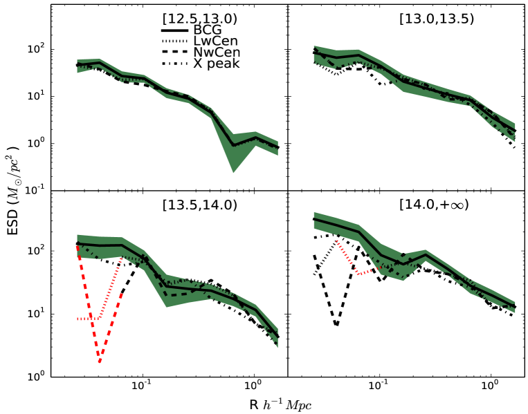
Shown in Fig. 2 are the ESD profiles measured around groups in different halo mass bins as indicated in each panel. In each panel, results are shown for different halo center tracers: BCG (black solid lines with one sigma error as green band), LwCen (black dotted line), NwCen (black dashed line) and X-ray peak position (black dash dotted line). Here the error bars are obtained by 2000 bootstrap resampling of the lens systems in consideration. The negative values from the measured ESDs are denoted by red color. At smaller scale , for more massive bins, the ESD signals around LwCen and NwCen begin to deviate from that of BCGs. Among these four types of halo center tracers, BCGs have the steepest ESD profiles at small scales, suggesting that BCGs are the best halo-center tracers.
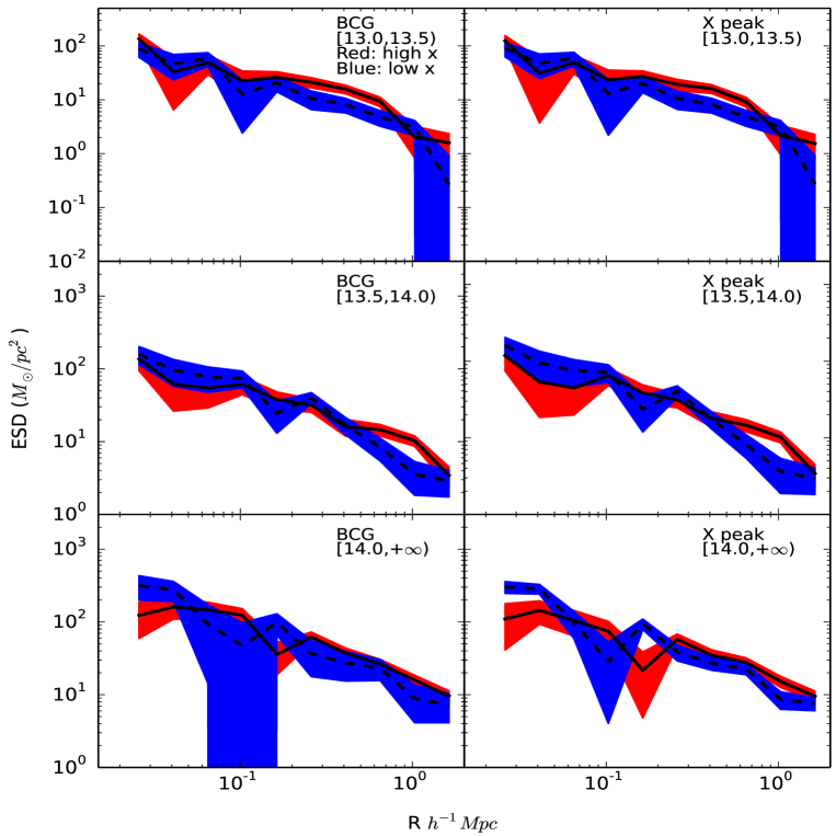
Shown in Fig. 3 are the ESDs measured from X-ray high and low luminosity groups. The solid curves with red one sigma error bands are the signals measured around high X-ray luminosity subsamples while the dashed lines with blue one sigma bands are results for low X-ray luminosity subsamples. There are some differences between the ESDs of high and low X-ray luminosity groups. In massive groups with mass , the low X-ray luminosity groups show somewhat more prominent ESDs at small scales, while in less massive groups the dependance is opposite. At large scales, the high X-ray luminosity groups show overall higher amplitude of ESDs indicating that the masses of their host halos are somewhat more massive.
3. The halo properties of galaxy groups
With the ESDs measured for different group samples and subsamples in previous section, we proceed to constrain the related halo properties of galaxy groups in this section.
3.1. Weak Lensing Model
The ESD around a lens galaxy is related to the line-of-sight projection of the galaxy-matter cross correlation function,
| (5) |
so that
| (6) |
and
| (7) |
where is the average background density of the Universe. Note that in both equations, we have omitted the contribution from the mean density of the universe, as it does not contribute to the ESD. In general, the ESD is composed of the following four components: host halo mass, subhalo mass if it is a satellite or interloper, the stellar mass associated with the galaxy in consideration and projected two halo term,
| (8) |
According to Yang et al. (2006a), if the candidate lens galaxy (system) locates at the center of host halo, the average projected density of the host halo can be calculated from the NFW profile. Assuming an NFW profile of the host halo, we have
| (9) |
with , where , . Here is the concentration parameter defined as the ratio between the virial radius of a halo and its characteristic scale radius . The projected surface density then can be analytically expressed as (Yang et al., 2006a):
| (10) |
where is the halo mass and bears the following form with :
| (11) |
On the other hand, if the candidate lens galaxy does not locate at the center of the host halo, but with an off-center distance , the projected surface density will change from an NFW profile to
| (12) |
Here, we adopt the offset model proposed by Johnston et al. (2007), where follows a 2D Gaussian distribution. This model is drawn from the mock catalog based on ADDGALS technique (Wechsler et al., 2006) combined with light-cone from Hubble Volume simulation (Evrard et al., 2002). The resulting projected density profile is the convolution between the and the ,
| (13) |
where
| (14) |
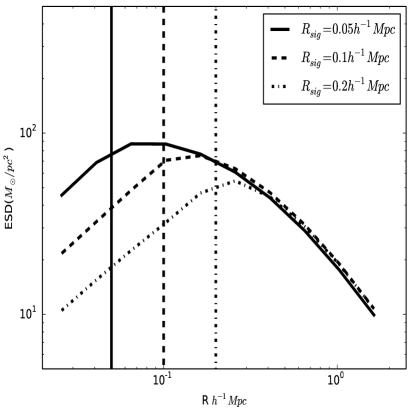
Here is the dispersion of . Thus in total, we have three free parameters regarding the host halo properties, , and , to be constrained using the observed ESDs. As an illustration, we show in the left panel of Fig. 4 how the measured ESDs may vary as a function of . Here we adopt a fixed halo mass and concentration with and based on Zhao et al. (2009) formula, and vary , respectively. Larger moves the ESD peak further away from measurement center, and suppress the signal at small scale.
Next, we consider the subhalo contribution. There is some possibility that the candidate lens galaxy is not the true central galaxy and may contain the subhalo component. In addition, in the group finder, there are some possibilities that the central galaxy is an interloper and may contain its original host halo component. For these reasons, we introduce a subhalo contribution in our ESD modelling. We assume that a fraction of contain subhalo with mass ,
| (15) |
Here we simply fix the concentration as 111As subhalos are on average relatively low mass ones and may be affected by stripping effect, their concentration is thus set to relatively large values. Change this value to 10 does not impact any of our results significantly. and treat and as our fourth and fifth free parameters in our modelling. In addition, we require that and .
Then we consider the stellar mass component. As pointed out in Johnston et al. (2007) and George et al. (2012), the stellar mass component can be treated as a point mass, and the related ESD can be modelled simply as,
| (16) |
where is the stellar mass of candidate central galaxy in consideration. We directly use the average stellar mass of galaxies as given in Table 1 and 2 in our modelling.
Finally, for the signal caused by the 2-halo term, we calculate the power spectrum at the mean redshift of each sample using the CAMB (Code for Anisotropies from Microwave Background ) of Lewis (2013) and then convert the power spectrum to matter-matter correlation function (Takahashi et al., 2012). is then related to halo-matter correlation function via halo bias model (Seljak & Warren, 2004)
| (17) |
To be more precise, we use the scale dependent bias model of Tinker et al. (2005),
| (18) |
where
| (19) |
The 2-halo term projected mass density is then calculated using Eqs. 4, 6 and 7. In practice, we only make the integration to a distance to model the 2-halo term contribution (see also Niemiec et al., 2017).
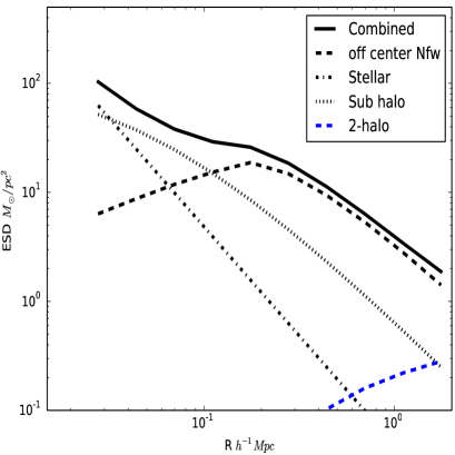
As an illustration, we show in the right panel of Fig. 4 each components of the model. Here we adopt and . The off-centered NFW is shown as the dashed line, stellar component as the dot-dashed line, sub halo as dotted line and the 2-halo term as the blue dashed line. The combined signal is the black solid curve. From this plot, we can see that at scales smaller than , stellar contribution becomes significant. The 2-halo term contribution is only important at scales larger than a few virial radii.
| Sample | Mass bin | Centers | |||||
|---|---|---|---|---|---|---|---|
| M1 | [12.5-13.0) | BCG | |||||
| M2 | [13.0-13.5) | BCG | |||||
| M3 | [13.5-14.0) | BCG | |||||
| M4 | [14.0-above) | BCG |
| Mass bin | Centers+X ray | |||||
|---|---|---|---|---|---|---|
| 13.0-13.5 | BCG+high | |||||
| BCG+low | ||||||
| X ray+high | ||||||
| X ray+low | ||||||
| 13.5-14.0 | BCG+high | |||||
| BCG+low | ||||||
| X ray+high | ||||||
| X ray+low | ||||||
| 14.0-above | BCG+high | |||||
| BCG+low | ||||||
| X ray+high | ||||||
| X ray+low |
3.2. Constrain halo properties using MCMC
In this subsection, we present our constraining of the halo properties using the above measured ESDs. There are five free parameters in our fitting process: host halo mass (), concentration (), off center distance (), subhalo mass (), and subhalo fraction (). We apply emcee (http://dan.iel.fm/emcee/current/) to run a Monte-Carlo Markov Chain (hereafter MCMC) to explore the likelihood function in the multi-dimensional parameter space222Emcee is an MIT licensed pure-Python implementation of Goodman & Weare’s Affine Invariant Markov chain Monte Carlo Ensemble sampler..
We assume a Gaussian likelihood function using convariance matrix built from bootstrap sampling,
| (20) |
where is the ESD data vector, is the model and is the inverse of the covariance matrix. denotes the parameters in the model.
In order to minimize the prior influence, we use broad flat priors for all five parameters. We set halo mass range for each fitting mass bin to be , concentration range , range and range . The only physical assumption on prior is that . The lower limit for is set since below which its ESD signal can be neglected. As we have seen in Fig 2 that the BCGs are the best tracers of the halo centers, we focus only this set of ESD measurements.
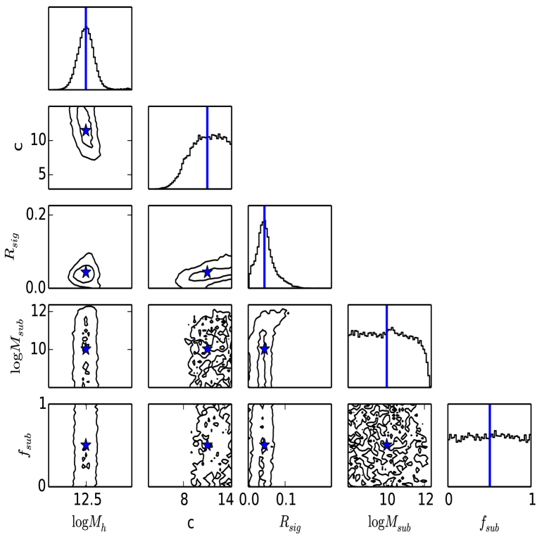
Fig. 5 is an example of marginalized posterior distributions of the five parameters for ESDs in the M1 sample after MCMC process. Within these five free parameters, we see only the host halo mass and the off-center distance can be well constrained. While concentration is quite strongly correlated with the off-center distance . The constraints on the subhalo fraction and subhalo mass is very weak.
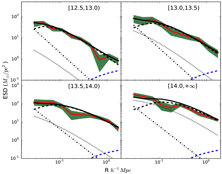
We show in Fig. 6 the best fitting results for groups separated in four different halo mass bins as well as the ESD contributions for different mass components. In the mass and radius ranges we consider, the subhalo and 2-halo term contributions are quite negligible. This is also the reason that we can’t make tight constraints on the subhalo fraction and subhalo mass. The contribution of stellar mass of the BCG is only important at very small scales. Thus the observed ESDs in this study can mainly provide us the constraints on the host halo properties.
Table 3 lists the best fitted parameters for groups in different mass bins. As we have seen from the likelihood distribution of parameters in Fig. 5, we can have fairly good constrain on the halo mass of the group samples. However, if we compare the halo masses obtained from the ESDs with those obtained from the group catalog (c.f. Table 1), they are roughly underestimated by 0.10.2 dex. We will discuss this discrepancy in the following section. The overall off-center distances for our BCGs are quite small, assuring that BCGs are indeed good tracers of halo centers. On the other hand, the concentrations of the halos seem to be somewhat larger than the theoretical predictions (e.g. Zhao et al., 2009). However, since the concentration and the off-center distance are quite tightly correlated, if we adopt the lower value of , the concentration will drop significantly as well.
Listed in Table 4 are the best fitted parameters for groups that are separated into X-ray luminosity high and low subsamples. Although, due to the smaller number of lens systems, the error for each data point for our X-ray subsamples are somewhat larger and thus the constraints on the five parameters are somewhat weaker, we do see a prominent feature that the halo masses of high X-ray luminosity subsamples are higher than their low luminosity counterparts in all mass bins. The difference is at 0.20.3 dex which means that the high X-ray luminosity subsamples are nearly by a factor of two more massive than their low X-ray luminosity counterparts.
4. Eddington bias of the halo mass estimation
Recent studies have shown that the combination of galaxy-galaxy lensing and clustering of galaxies can be used to constrain cosmology (e.g. van den Bosch et al., 2013; More et al., 2013; Cacciato et al., 2013; Leauthaud et al., 2017), the halo masses estimated for groups using galaxy-galaxy lensing signals and hence the halo mass function can also be used to constrain the cosmological parameters. However, before doing so, one needs to make a careful study of the systematics between the galaxy-galaxy lensing measurement and modelling. Note that the group masses estimated from the ranking of characteristic group luminosity or stellar mass have a typical uncertainty at about 0.3 dex. Thus the halos/groups binned in terms of group mass may induce an Eddington bias in the galaxy-galaxy lensing halo mass estimation.
Here we make use of a high resolution N-body simulation to help us understanding the systematics of galaxy-galaxy lensing modelling. Our simulation includes dark matter particles in a periodic box of on a side (Li et al., 2016), which was carried out at the Center for High Performance Computing at Shanghai Jiao Tong University. It was run with L-GADGET, a memory-optimized version of GADGET2 (Springel, 2005). The cosmological parameters adopted by this simulation are consistent with the WMAP9 results (Hinshaw et al., 2013) (which are very similar to WMAP7 results as well), and each particle has a mass of . Dark matter halos are identified using the standard friends-of-friends algorithm with a linking length that is 0.2 times the mean inter particle separation. The mass of halos, , is simply defined as the sum of the masses of all the particles in the halos, and we remove halos with less than 20 particles.
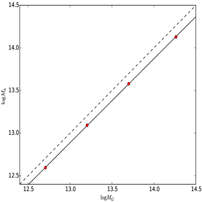
Using the true halos in the simulation, we mimic the halo mass estimation uncertainty in the groups as follows. First, we add to each halo mass a Gaussian scatter with in log space. Next, we rank all the resulting halos and match them with the halo mass function model prediction (Tinker et al., 2008) assuming a WMAP7 cosmology to assign each halo a new mass. Thus assigned halo masses are referred to as the group masses . Following the same mass selection criteria used for our galaxy-galaxy lensing studies, we separate the groups (halos) into four samples. From these four samples, we estimated both the average group mass and the true halo mass . The resulting group v.s. true halo mass relation is shown in the left panel of Fig. 7. Obviously, the data points are off from the diagonal dotted line at about 0.1 dex level, which illustrates a bias between these two halo masses. We use a solid line to fit the data points, which can be used to roughly account for the Eddington bias in our weak galaxy-galaxy lensing studies.
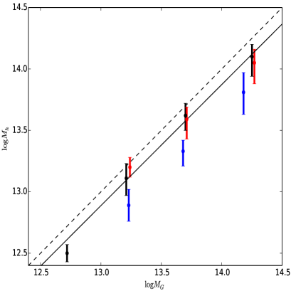
Shown in the right panel of Fig. 7 is the average group mass v.s. the true halo mass estimated from the galaxy-galaxy lensing signals in our study. For all the group sample, after taking into account the Eddington bias, i.e. comparing to the solid line, the data in the three massive group bins agree very well. Indicating the WMAP7 cosmology adopt in this study is quite consistent with the lensing mass constraints. On the other hand, according to the result for the lowest mass bin, we still see that the halo mass estimated from the galaxy-galaxy lensing signals is about 0.1 dex lower. Similar trends were also reported in a recent study by Leauthaud et al. (2017), where they found that the lensing signals predicted from clustering are 20%-40% larger than the true measurements. It still remains unclear to us what is the main cause of this lensing deficiency around relatively low mass halos.
While for the groups that are separated into X-ray luminosity high and low subsamples, we do see that the average halo masses of X-ray luminosity low subsamples are systematically smaller. Thus a combination of X-ray luminosity and optical total group luminosity will be useful to better constrain the individual group/cluster mass.
Finally, we caution that when using galaxy-galaxy lensing signals around lens systems to constrain cosmological parameters in future larger surveys, it would be important to take into account the Eddington bias as demonstrated here.
5. Summary and Conclusion
We measure the galaxy-galaxy lensing signals around group samples in different mass bins using the source galaxy shape measurements obtained by Luo et al. (2017), where the group masses are provided by Yang et al. (2007) using the ranking of characteristic group luminosity. We also divide the groups with X-ray luminosities obtained by Wang et al. (2014) into X-ray luminosity high and low subsamples, and measured their galaxy-galaxy lensing signals separately.
We then model the galaxy-galaxy signals by considering contributions from an off-centered NFW profile, sub halo, stellar mass and 2-halo term using five free parameters: halo mass , concentration , off-center distance , subhalo fraction and the subhalo mass . We then run MCMC to constrain the five free parameters by assigning them with flat priors. From the lensing signals we measured from the SDSS DR7 observation, we are able to provide relatively good constraints on the halo properties, however not the subhalo properties. Below we summarize the main findings of this work.
-
•
By checking the galaxy-galaxy lensing signals around four kinds of halo center tracers: BCG, luminosity weighted center, number weighted center and X-ray peak position, we find that BCG is the best halo center tracer.
-
•
The off-center effect for BCG is roughly at , from for the lowest mass bin group sample to for the most massive group sample.
-
•
After taking into account the Eddington biasThe, halo masses estimated from galaxy-galaxy lensing signals are consistent with the group masses obtained using abundance matching assuming WMAP7 cosmology in the three massive samples. This consistency implies that the WMAP7 cosmology is favored by the lensing signals measured in this study.
-
•
If separated into X-ray luminosity high and low subsamples, X ray luminosity low subsamples have overall lower halo masses compared to their X ray luminosity high counterparts. This X-ray luminosity segregation in halo mass indicates that we can combine X ray luminosities and optical luminosities of groups to better constrain their individual masses.
Finally, as the galaxy-galaxy lensing can provide us an independent measurement of the halo mass for clusters and groups, for larger and deeper surveys, we can use the resulting halo mass functions to constrain cosmological parameters.
References
- Abazajian et al. (2009) Abazajian, K. N., Adelman-McCarthy, J. K., Agüeros, M. A., et al. 2009, ApJS, 182, 543
- Bacon & Taylor (2003) Bacon, D. J., & Taylor, A. N. 2003, MNRAS, 344, 1307
- Bell et al. (2003) Bell, E. F., McIntosh, D. H., Katz, N., & Weinberg, M. D. 2003, ApJS, 149, 289
- Bernstein & Jarvis (2002) Bernstein, G. M., & Jarvis, M. 2002, AJ, 123, 583
- Bernstein & Armstrong (2014) Bernstein, G. M., & Armstrong, R. 2014, MNRAS, 438, 1880
- Bertin & Arnouts (1996) Bertin, E., & Arnouts, S. 1996, A&AS, 117, 393
- Blanton et al. (2005) Blanton, M. R., Schlegel, D. J., Strauss, M. A., et al. 2005, AJ, 129, 2562
- Bleem et al. (2015) Bleem, L. E., Stalder, B., de Haan, T., et al. 2015, ApJS, 216, 27
- Bridle et al. (2002) Bridle, S. L., Kneib, J.-P., Bardeau, S., & Gull, S. F. 2002, The Shapes of Galaxies and their Dark Halos, 38
- Cacciato et al. (2009) Cacciato, M., van den Bosch, F. C., More, S., et al. 2009, MNRAS, 394, 929
- Cacciato et al. (2013) Cacciato, M., van den Bosch, F. C., More, S., Mo, H., & Yang, X. 2013, MNRAS, 430, 767
- Eke et al. (2004) Eke, V. R., Baugh, C. M., Cole, S., et al. 2004, MNRAS, 348, 866
- Evrard et al. (2002) Evrard, A. E., MacFarland, T. J., Couchman, H. M. P., et al. 2002, ApJ, 573, 7
- Fischer et al. (2000) Fischer, P., McKay, T. A., Sheldon, E., et al. 2000, AJ, 120, 1198
- Fu et al. (2008) Fu, L., Semboloni, E., Hoekstra, H., et al. 2008, A&A, 479, 9
- George et al. (2012) George, M. R., Leauthaud, A., Bundy, K., et al. 2012, ApJ, 757, 2
- Heymans et al. (2005) Heymans, C., Brown, M. L., Barden, M., et al. 2005, MNRAS, 361, 160
- Heymans et al. (2012) Heymans, C., Van Waerbeke, L., Miller, L., et al. 2012, MNRAS, 427, 146
- Hinshaw et al. (2013) Hinshaw, G., Larson, D., Komatsu, E., et al. 2013, ApJS, 208, 19
- Hirata & Seljak (2003) Hirata, C., & Seljak, U. 2003, MNRAS, 343, 459
- Johnston et al. (2007) Johnston, D. E., Sheldon, E. S., Tasitsiomi, A., et al. 2007, ApJ, 656, 27
- Kaiser et al. (1995) Kaiser, N., Squires, G., & Broadhurst, T. 1995, ApJ, 449, 460
- Kitching et al. (2008) Kitching, T. D., Miller, L., Heymans, C. E., van Waerbeke, L., & Heavens, A. F. 2008, MNRAS, 390, 149
- Kilbinger et al. (2013) Kilbinger, M., Fu, L., Heymans, C., et al. 2013, MNRAS, 430, 2200
- Koester et al. (2007) Koester, B. P., McKay, T. A., Annis, J., et al. 2007, ApJ, 660, 221
- Kuijken et al. (2015) Kuijken, K., Heymans, C., Hildebrandt, H., et al. 2015, MNRAS, 454, 3500
- Leauthaud et al. (2010) Leauthaud, A., Finoguenov, A., Kneib, J.-P., et al. 2010, ApJ, 709, 97
- Leauthaud et al. (2017) Leauthaud, A., Saito, S., Hilbert, S., et al. 2017, MNRAS, 467, 3024
- Lewis (2013) Lewis, A. 2013, Phys. Rev. D, 87, 103529
- Li et al. (2016) Li, R., Shan, H., Kneib, J.-P., et al. 2016, MNRAS, 458, 2573
- LSST Science Collaboration et al. (2009) LSST Science Collaboration, Abell, P. A., Allison, J., et al. 2009, arXiv:0912.0201
- Lu et al. (2015) Lu, Y., Yang, X., & Shen, S. 2015, ApJ, 804, 55
- Luo et al. (2017) Luo, W., Yang, X., & Zhang, J. 2017, ApJ, 836, 1
- Lupton et al. (2001) Lupton, R., Gunn, J. E., Ivezić, Z., Knapp, G. R., & Kent, S. 2001, Astronomical Data Analysis Software and Systems X, 238, 269
- Jarvis et al. (2015) Jarvis, M., Sheldon, E., Zuntz, J., et al. 2015, arXiv:1507.05603
- Mandelbaum et al. (2005) Mandelbaum, R., Hirata, C. M., Seljak, U., et al. 2005, MNRAS, 361, 1287
- Mandelbaum et al. (2006) Mandelbaum, R., Seljak, U., Kauffmann, G., Hirata, C. M., & Brinkmann, J. 2006, MNRAS, 368, 715
- Maoli et al. (2000) Maoli, R., Mellier, Y., van Waerbeke, L., et al. 2000, The Messenger, 101, 10
- Miller et al. (2005) Miller, C. J., Nichol, R. C., Reichart, D., et al. 2005, AJ, 130, 968
- Miller et al. (2007) Miller, L., Kitching, T. D., Heymans, C., Heavens, A. F., & van Waerbeke, L. 2007, MNRAS, 382, 315
- Miller et al. (2013) Miller, L., Heymans, C., Kitching, T. D., et al. 2013, MNRAS, 429, 2858
- More et al. (2013) More, S., van den Bosch, F. C., Cacciato, M., et al. 2013, MNRAS, 430, 747
- Niemiec et al. (2017) Niemiec, A., Jullo, E., Limousin, M., et al. 2017, arXiv:1703.03348
- Pratt et al. (2009) Pratt, G. W., Croston, J. H., Arnaud, M., & Böhringer, H. 2009, A&A, 498, 361
- Refregier (2003) Refregier, A. 2003, ARA&A, 41, 645
- Refregier et al. (2010) Refregier, A., Amara, A., Kitching, T. D., et al. 2010, arXiv:1001.0061
- Rhodes et al. (2000) Rhodes, J., Refregier, A., & Groth, E. J. 2000, ApJ, 536, 79
- Rykoff et al. (2014) Rykoff, E. S., Rozo, E., Busha, M. T., et al. 2014, ApJ, 785, 104
- Seljak & Warren (2004) Seljak, U., & Warren, M. S. 2004, MNRAS, 355, 129
- Sheldon et al. (2004) Sheldon, E. S., Johnston, D. E., Frieman, J. A., et al. 2004, AJ, 127, 2544
- Simet et al. (2016) Simet, M., McClintock, T., Mandelbaum, R., et al. 2016, arXiv:1603.06953
- Springel (2005) Springel, V. 2005, MNRAS, 364, 1105
- Sunyaev & Zeldovich (1972) Sunyaev, R. A., & Zeldovich, Y. B. 1972, Comments on Astrophysics and Space Physics, 4, 173
- Takahashi et al. (2012) Takahashi, R., Sato, M., Nishimichi, T., Taruya, A., & Oguri, M. 2012, ApJ, 761, 152
- Tinker et al. (2005) Tinker, J. L., Weinberg, D. H., Zheng, Z., & Zehavi, I. 2005, ApJ, 631, 41
- Tinker et al. (2008) Tinker, J., Kravtsov, A. V., Klypin, A., et al. 2008, ApJ, 688, 709-728
- van den Bosch et al. (2004) van den Bosch, F. C., Norberg, P., Mo, H. J., & Yang, X. 2004, MNRAS, 352, 1302
- van den Bosch et al. (2013) van den Bosch, F. C., More, S., Cacciato, M., Mo, H., & Yang, X. 2013, MNRAS, 430, 725
- Viola et al. (2015) Viola, M., Cacciato, M., Brouwer, M., et al. 2015, MNRAS, 452, 3529
- van Waerbeke (2001) van Waerbeke, L. 2001, Cosmological Physics with Gravitational Lensing, 165
- Wang et al. (2014) Wang, L., Yang, X., Shen, S., et al. 2014, MNRAS, 439, 611
- Wechsler et al. (2006) Wechsler, R. H., Zentner, A. R., Bullock, J. S., Kravtsov, A. V., & Allgood, B. 2006, ApJ, 652, 71
- Yang et al. (2005) Yang, X., Mo, H. J., van den Bosch, F. C., & Jing, Y. P. 2005, MNRAS, 356, 1293
- Yang et al. (2006a) Yang, X., Mo, H. J., van den Bosch, F. C., et al. 2006a, MNRAS, 373, 1159
- Yang et al. (2006b) Yang, X., Mo, H. J., & van den Bosch, F. C. 2006b, ApJ, 638, L55
- Yang et al. (2007) Yang, X., Mo, H. J., van den Bosch, F. C., et al. 2007, ApJ, 671, 153
- York et al. (2000) York, D. G., Adelman, J., Anderson, J. E., Jr., et al. 2000, AJ, 120, 1579
- Zhang (2010) Zhang, J. 2010, MNRAS, 403, 673
- Zhang (2011) Zhang, J. 2011, JCAP, 11, 041
- Zhang et al. (2015) Zhang, J., Luo, W., & Foucaud, S. 2015, JCAP, 1, 024
- Zhang (2016) Zhang, J 2016, National Science Review, 3, 159-164
- Zhao et al. (2009) Zhao, D. H., Jing, Y. P., Mo, H. J., Börner, G. 2009, ApJ, 707, 354
- Zu et al. (2014) Zu, Y., Weinberg, D. H., Jennings, E., Li, B., & Wyman, M. 2014, MNRAS, 445, 1885
- Zu & Weinberg (2013) Zu, Y., & Weinberg, D. H. 2013, MNRAS, 431, 3319