Interacting passive advective scalars in an active medium

Abstract

Recent experimental studies, both in vivo and in vitro, have revealed that membrane components that bind to the cortical actomyosin meshwork are driven by active fluctuations, whereas membrane components that do not bind to cortical actin are not. Here we study the statistics of density fluctuations and dynamics of particles advected in an active quasi-two dimensional medium comprising self-propelled filaments with no net orientational order, using a combination of agent-based Brownian dynamics simulations and analytical calculations. The particles interact with each other and with the self-propelled active filaments via steric interactions. We find that the particles show a tendency to cluster and their density fluctuations reflect their binding to and driving by the active filaments. The late-time dynamics of tagged particles is diffusive, with an active diffusion coefficient that is independent of (or at most weakly-dependent on) temperature at low temperatures. Our results are in qualitative agreement with the experiments mentioned above. In addition, we make predictions that can be tested in future experiments.

I Introduction and Motivation

The spatial organization, clustering and dynamics of many cell surface molecules is influenced by interaction with the actomyosin cortex raomayor ; Goswami ; kripa ; saha ; Hancock ; Lingwood , a thin layer of actin cytoskeleton and myosin motors, measured to be around $250$ nm in HeLa cells Paluch , that is juxtaposed with the membrane bilayer. Although the ultrastructure of the cortical actin cytoskeleton is as yet poorly defined, there is growing evidence that it is composed simultaneously of dynamic filaments kripa and an extensively branched static meshwork Morone . The coupling of the membrane to these two types of actin configurations is expected to affect the dynamics and organization of membrane components, presumably in different ways.

A common feature of these cell surface proteins is that they can bind, directly or indirectly, to cortical actin. As a consequence, the action of myosin motors on actin at the cortex help drive the local clustering and dynamics of these cell surface proteins. Mutations of these proteins that abrogate this actin binding capacity, leave them unaffected by the dynamics of the actomyosin cortex kripa ; saha . Similarly, silencing myosin motor activity, renders the dynamics of these cell surface proteins normal and akin to their mutated counterpart kripa ; saha . A description of the cell surface as an Active Composite of a multicomponent, asymmetric bilayer juxtaposed with a thin cortical actomyosin layer (Fig. 1), appears to consistently explain the anomalous dynamical features of these proteins raomayor ; kripa ; saha . In these earlier studies  kripa ; kripasoft , we had used a coarse grained description, based on active hydrodynamics rmp . Recently, it has been shown that much of this behaviour is recapitulated in a minimal in vitro reconstitution of a supported bilayer in contact with a thin layer of short actin filaments and Myosin-II minifilaments, driven by the hydrolysis of ATP darius . The success of this minimal setup motivates us to revisit our continuum hydrodynamic description from a more microscopic standpoint. Our present study is an agent-based Brownian dynamics simulation of a mixture of polar active filaments and passive particles which interact with each other. Since the parameter space for exploration is large, we restrict our study here to the case where the density of filaments and particles is low (negligible filament overlap), and where there is no net orientational order.

For the present purposes, we schematically represent the Active Composite Cell Surface, as in Fig. 1. To enable a systematic study, we conceptually separate out the different architectures of actin at the cortex - (i) where the cortical layer consists of only short dynamic filaments described as an active fluid (the subject of the present paper) and (ii) where the cortical layer consists of only long filaments forming a static mesh of characteristic mesh size $\xi\approx 52$ nm in FRSK cells Morone ; fujiwara (which we take up in a later publication). In future, we will combine these configurations into a single model of the cortical actomyosin.

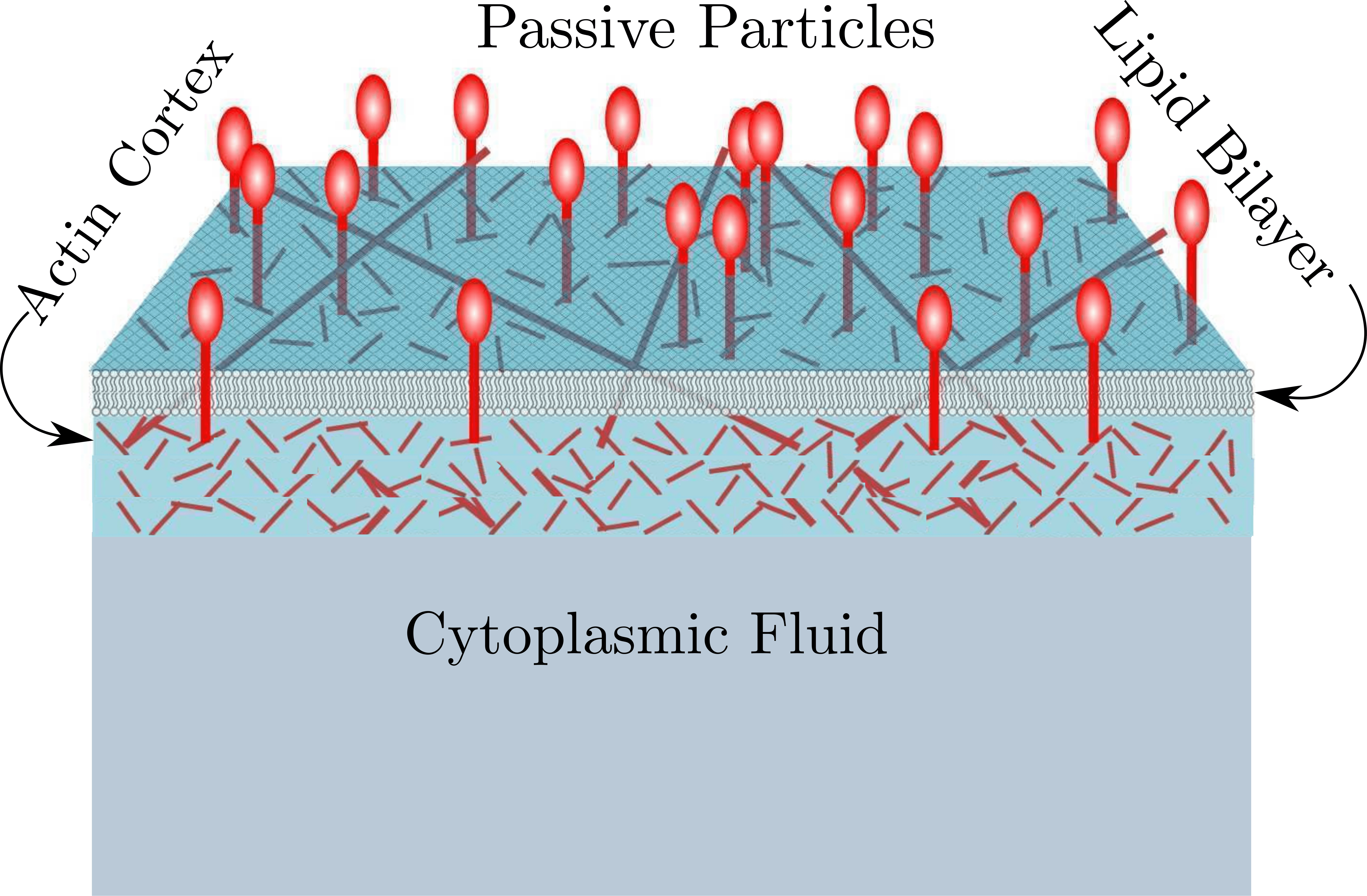
Figure 1: Schematic of the Active Composite Cell Surface with a multicomponent asymmetric bilayer membrane juxtaposed with the cortical layer of actin and myosin. The actin layer consists of short dynamic actin and long static actin filaments, the latter forming a crosslinked mesh Morone ; fujiwara . For clarity, myosin motors are not shown, the short filaments are active and represent myosin bound actin filaments. The passive molecules (shown in red) are transmembrane proteins that have a cytoplasmic actin-binding domain.

Our choice of Brownian dynamics simulations is motivated by experiments on tagged particle diffusion both on the cell surface and in the in vitro reconstitution. Molecules that bind to dynamic actin (passive molecules) are affected by the active fluctuations of actomyosin - their diffusion shows anomalous behaviour strongly indicative of active driving. On the other hand, molecules that do not interact with actin (inert molecules), such as short chain lipids and proteins whose actin-binding domain has been mutated so as to abrogate their interaction with actin, do not show any influence of active fluctuations kripa ; saha ; darius . There appears to be no sign that the transport of these inert molecules is affected by potential hydrodynamic flows induced by active stresses coming from actomyosin yhat ; abasu .

While our primary motivation are the experimental studies of the tagged particle dynamics on the cell surface, our work is also relevant to transport in other living and nonliving systems, as long as the effects of hydrodynamics are negligible, for instance, to the movement of multiple motor-driven cargo vesicles or synthetic beads on the cytoskeletal network Grannick .

II Brownian dynamics and characterization

II.1 Simulation details

We study the dynamics of a mixture of polar active filaments and passive particles using an agent-based Brownian dynamics simulation. The passive particles are modelled as mono-disperse soft spheres of diameter $\sigma$. A pair of passive particles separated by a distance $r$ interact via a truncated Lennard Jones (LJ) pair potential of the form,

$$V_{pp}(r) = 4\epsilon\Bigg{[}\bigg{(}\frac{\sigma}{r}\bigg{)}^{12}-\bigg{(}\frac{\sigma}{r}\bigg{)}^{6}\Bigg{]}+V_{0}+V_{2}r^{2}\,\,\,\,\,\mbox{for}\,\,r\leq r_{c}$$ (1)

$$= 0\,\,\,\,\,\mbox{for}\,\,r>r_{c}$$

where $r_{c}=2.5\sigma$ and values of $V_{0}$ and $V_{2}$ are chosen so that the potential and force are continuous at the truncation point. We set $\sigma=1$ and $\epsilon=1$ to be the units of length and energy, respectively.

The polar filaments are modelled as semi-flexible bead-spring polymers, with both stretch and bend distortions. We implement excluded volume interaction between the beads of same filament, as well as between two different filaments through a truncated Lennard Jones pair potential of the form,

$$V_{bb}(r) = 4\epsilon^{\prime}\Bigg{[}\bigg{(}\frac{\sigma^{\prime}}{r}\bigg{)}^{12}-\bigg{(}\frac{\sigma^{\prime}}{r}\bigg{)}^{6}\Bigg{]}+V_{0}^{\prime}+V_{2}^{\prime}r^{2}\,\,\,\,\,\mbox{for}\,\,r\leq r^{\prime}_{c}$$ (2)

$$= 0\,\,\,\,\,\mbox{for}\,\,r>r^{\prime}_{c}$$

where $r$ is the distance between the centres of the corresponding beads, $r^{\prime}_{c}=2^{1/6}\sigma^{\prime}$ and $V_{0}^{\prime},V_{2}^{\prime}$ are constants, chosen so that the potential and force are continuous at $r^{\prime}_{c}$. We take $\sigma^{\prime}=2$ and $\epsilon^{\prime}=1$. Each filament is composed of $10$ beads and therefore has an equilibrium length $l_{0}=20$, in the units of $\sigma$.

Note that with our choice of cutoffs, the particle-particle interaction $V_{pp}$ has both attractive and repulsive parts, whereas the bead-bead interaction $V_{bb}$ is strictly repulsive.

To make the filament semi-flexible, we impose additional spring forces on the beads. A harmonic stretching potential with spring constant $K_{c}=400$, in units of $\epsilon/\sigma^{2}$, ensures that the length of the filament does not deviate significantly from its equilibrium value, $l_{0}=20$. The bending energy of a triplet of connected beads is also harmonic in the angle, with a bending stiffness $K_{a}=600$, in units of $\epsilon$. This high $K_{a}$ makes the filaments very stiff, with a typical persistence length much larger than $l_{0}$.

A propulsion force ${\bf f}=f_{0}{\bf{\hat{n}}}$ is imposed on each of the beads, along the average direction (${\bf{\hat{n}}}$) of all the bonds present in a filament. Note that we do not impose any filament alignment rule nor do we prescribe any activity decorrelation time. Instead, these originate from thermal fluctuations on the constituent monomers comprising each filament and collisions driven by thermal and active forces, an emergent many-particle feature. As a consequence, both the local alignment and orientational de-correlation time are functions of temperature, density and activity.

The interactions between the beads of the filament and the passive particles are modelled by a harmonic potential of spring constant $K_{s}=50$ in units of $\epsilon/\sigma^{2}$. The harmonic potential is truncated at a cutoff distance $r_{0}=1$ and set to zero beyond it. When a passive particle comes within a distance $r_{0}$ from the centre of a filament bead, it binds to the corresponding bead and gets advected along with the filament, under the application of propulsion force $f_{0}{\bf{\hat{n}}}$.

Unless mentioned otherwise, all results presented here are for $N_{p}=800$ passive particles and $N_{r}=50$ self-propelled filaments in a two dimensional area of linear dimension $L=396.4$. For most of the study, we take the area fractions of the rods ($c$) and particles ($\rho$) to be $c=0.01$ and $\rho=0.004$, respectively.

The Brownian dynamics equations involve an update of both the passive particle and the filament bead coordinates, for which we have used a simple Euler integration scheme with integration time step $\Delta t\sim 10^{-4}$. The dynamics of the particle coordinates is given by

$$\dot{\bf r}_{i}^{p}=\begin{cases}-\gamma^{-1}_{p}{\bm{\nabla}}_{i}V_{p}+\sqrt{2k_{B}T/\gamma_{p}}{\bm{\xi}}_{i},&\text{(unbound)}\\ -\gamma^{-1}_{p}{\bm{\nabla}}_{i}V_{p}+\sqrt{2k_{B}T/\gamma_{p}}{\bm{\xi}}_{i}+{\bf f}_{i}/\gamma_{p},&\text{(bound)}\end{cases}$$ (3)

where $\gamma_{p}$ is the friction coefficient of the passive particle, $V_{p}$ is the net potential felt by the $i$-th passive particle and includes contributions from Eq. 1 and the bead-particle spring interactions. The diffusion of the unbound particle is driven by a thermal noise ${\bm{\xi}}_{i}$ with zero mean and unit variance acting on $i$-th particle. On the other hand, the bound particles are subject to both the thermal noise and active driving.

The dynamics of the filament-bead coordinates is given by

$$\dot{\bf r}_{j}^{b}=-\gamma^{-1}_{b}{\bm{\nabla}}_{j}V_{b}+\sqrt{2k_{B}T/\gamma_{b}}\,{\bm{\xi}}_{j}+{\bf f}_{j}/\gamma_{b}\,$$ (4)

where $\gamma_{b}$ is the friction coefficient of the bead, $V_{b}$ is the net potential felt by the $j$-th bead and includes contributions from Eq. 2, harmonic stretching and bending interactions.

We take $\gamma_{p}=1$, which together with $\sigma=1$ and $\epsilon=1$, sets the units of space, time and energy. All other quantities can be written in terms of these units, so as to make Eqs. 3, 4 dimensionless. In all that follows below, except in Sec. V, we have taken $\gamma_{b}=\gamma_{p}$. To be able to make contact with experiments, we have to translate our simulation units (S.U.) to real units (R.U.). Setting $\sigma=10$ nm, $\gamma=0.123$ pN ${\mu m}^{-1}$ s kamm and $\epsilon=4.14\times 10^{-21}$ J, we can convert our simulation units to real units, as displayed in Table 1.

We have typically run the Brownian dynamics simulation for a total time $t\sim 10^{4}$, ensuring that the system has reached steady state. We have varied the temperature over $T=0.25,0.5,0.75,1,2,4,6,8,10,15,25$ and the propulsion force over $f_{0}=0.0,0.5,1.0,2.0,3.0,4.0$. Our initial conditions are chosen from a thermal distribution at temperature $T$ and all results presented here are averaged over $16$ such independent initial realisations.

II.2 Statistics of filament orientation

We characterise the $i$-th filament by its centre of mass position ${\bf r}_{i}$ and a unit vector ${\bf n}_{i}=(\cos\theta_{i},\sin\theta_{i})$ along its long axis to describe its polar orientation (recall that the filaments are very stiff). We first ensure that the configuration of filaments is in the spatially homogeneous, orientationally isotropic state - this is demonstrated in the plots of the probability distribution of the polar $P(\theta)$ and nematic orientations $P(\tilde{\theta})$ (Fig. 2).

Table 1: Conversion between simulation units (S.U.) and real units (R.U.)

$Parameter[Dimension]$	$S.U.$	$R.U.$
$\sigma$ [$l$]	1	$10$ $nm$
$\epsilon$ [$ml^{2}t^{-2}$]	1	$4.14\times 10^{-21}$ $J$
$\gamma_{p}$ [$mt^{-1}$]	1	$0.123$ $pN{\mu m}^{-1}s$
$T$ [$k$]	1	$300$ $K$
$t$ [$t$]	1	$3\times 10^{-3}$ $s$
$k_{u},k_{b}$ [$t^{-1}$]	1	$333$ $s^{-1}$
$f_{0}$ [$mlt^{-2}$]	1	$0.41$ $pN$
$V_{a}$ [$lt^{-1}$]	1	$3.3$ $\mu m$ $s^{-1}$
$K_{c}$ [$mt^{-2}$]	1	$41.4$ $pN{\mu m}^{-1}$
$K_{a}$ [$ml^{2}t^{-2}$]	1	$4.14\times 10^{-21}$ $J$
$K_{s}$ [$mt^{-2}$]	1	$41.4$ $pN{\mu m}^{-1}$
$D$ [$l^{2}t^{-1}$]	1	$3.3\times 10^{-2}$ ${\mu m}^{2}/s$

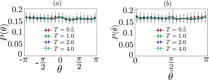
Figure 2: Normalised distribution of (a) polar orientation $P(\theta)$ and (b) nematic orientation $P({\tilde{\theta}})$, of the filaments at different temperature $T$ with activity $f_{0}=4.0$, showing that the system is in the isotropic phase for a representative set of parameters.

We then calculate the orientational correlation lengths, so as to ensure that this is much smaller than our system size and comparable to the size of the filaments. To do this, we calculate the spatial correlations of both the polar and nematic orientation,

$$C_{P}(r) = \Bigg{\langle}\frac{1}{N^{2}}\sum_{i=1}^{N}\sum_{j=1}^{N}\cos(\theta_{i}-\theta_{j})\Bigg{\rangle}$$ (5)

$$C_{N}(r) = \Bigg{\langle}\frac{1}{N^{2}}\sum_{i=1}^{N}\sum_{j=1}^{N}(2\cos^{2}(\theta_{i}-\theta_{j})-1)\Bigg{\rangle}$$ (6)

where $r=|{\bf r}_{i}-{\bf r}_{j}|$ is the distance between the centre-of-mass of the $i$-th and $j$-th filaments. By fitting this to an exponential (Figs. 3 and 4), we extract the polar and nematic orientation correlation lengths, $\zeta_{P}$ and $\zeta_{N}$, whose dependence on the area fraction of filaments $c$ (we will henceforth refer to this as filament density) is shown in the inset.

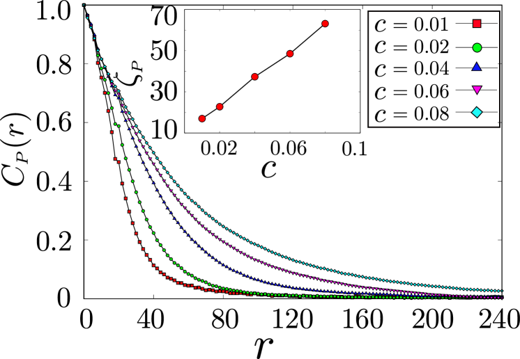
Figure 3: Spatial correlation of the polar orientation, $C_{P}(r)$, of the filaments at different filament densities $c$ at $T=0.5$ and active propulsion $f_{0}=4$. Inset shows the corresponding correlation length $\zeta_{P}$ as a function of filament density $c$.

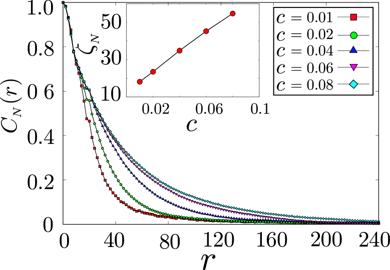
Figure 4: Spatial correlation of the nematic orientation, $C_{N}(r)$, of the filaments at different filament density $c$ at $T=0.5$ and $f_{0}=4$. Inset shows the corresponding correlation length $\zeta_{N}$ as a function of filament density $c$.

Throughout the paper (unless mentioned otherwise) we work at a filament density of $c=0.01$, and temperatures $T\geq 0.5$; in this regime, the orientational correlation lengths are of the order of the filament length, $l_{0}$, and hence comfortably within the isotropic phase.

II.3 Statistics of filaments persistence

A self-propelled filament moves persistently in a direction set by ${\bf V}_{a}=\frac{f_{0}\bf{\hat{n}}}{\gamma_{b}}$, taken to be along its polar orientation, until its orientation gets decorrelated, either due to thermal noise on the individual monomers constituting the filaments or due to inter-filament collisions. What is the spatial correlation of these directions of persistent motion? Here, we calculate this velocity orientation correlation function $C_{V}(r)$ at different $T$ (Fig. 5) using the formula

$$C_{V}(r) = \Bigg{\langle}\frac{1}{N^{2}}\sum_{i=1}^{N}\sum_{j=1}^{N}(2\cos^{2}(\Theta_{i}-\Theta_{j})-1)\Bigg{\rangle}$$ (7)

where $\Theta_{i}$ represents the direction of the velocity vector of the $i$-th filament. From this spatial correlation function $C_{V}(r)$ we extract a correlation length ($\zeta_{V}$) which measures the spatial extent of the persistent dynamics. We find again that at $c=0.01$ over the temperature range $T\geq 0.5$, the correlation length $\zeta_{V}$ is comparable with the filament length $l_{0}$.

Figure 5: Spatial correlation of the direction of persistent movement of the filaments, measured by the velocity orientation correlation function $C_{V}(r)$, at different temperatures, with the filament density $c=0.01$ and propulsion force $f_{0}=4$. Inset shows the corresponding correlation length $\zeta_{V}$ as a function of $T$.

II.4 Statistics of binding-unbinding of passive particles onto filaments

The dynamical equations (3) and (4) are written entirely in terms forces, either active or derived from a potential, and thermal noise. The particles experience a binding and unbinding onto the filaments which depend on this interplay between thermal noise and the attractive potentials. Thus for instance, the unbound passive particles diffuse in the two dimensional medium and ever so often come within the vicinity ($r\leq r_{0}=1$) of a moving filament-bead, whereupon they bind to the filament-bead. In the low density limit, we expect the binding rate $k_{b}$ to be diffusion limited and so $k_{b}\propto T$ and independent of $K_{s}$ where $K_{s}$ is the strength of trapping harmonic interaction.

To study the unbinding of a particle bound from a filament-bead, we compute the rate of escape of a particle trapped in a truncated attractive harmonic potential grebenkov , parametrised by $K_{s}$ and $r_{0}$. This is given by

$$k_{u}=\frac{K_{s}^{2}r_{0}^{2}}{\gamma_{p}k_{B}T}\,\exp\left(-\frac{K_{s}r_{0}^{2}}{2k_{B}T}\right)$$ (8)

and should be a good description of the dynamics of unbinding of the passive particles in the limit of low particle density.

We compare these theoretical estimates with the results of simulations on a mixture of particles and filaments at equilibrium (no active propulsion), from which we extract the values of $k_{u}$ and $k_{b}$ in two different ways. In the first method, we represent the stochastic binding and unbinding by a telegraphic process kampen , characterised by a mean duty ratio,

$$\langle\phi\rangle=\frac{k_{b}}{k_{b}+k_{u}}\,,$$ (9)

the fraction of time spent by the tagged particle in the bound state over the observation time, and a two-point correlator,

$$\langle\phi(t)\phi(t^{\prime})\rangle=\langle\phi\rangle^{2}+\langle\phi\rangle\left(1-\langle\phi\rangle\right)e^{-2\frac{|t-t^{\prime}|}{t_{sw}}}$$ (10)

where

$$t_{sw}=\frac{2}{k_{b}+k_{u}}\,,$$ (11)

is called the mean switching time and describes the mean time taken to switch from a bound to an unbound state. We calculate $k_{b}$ and $k_{u}$, by fitting our simulation results to $\langle\phi\rangle$ and $\langle\phi(t)\phi(t^{\prime})\rangle$. In the second method, we calculate $k_{u}$ ($k_{b}$) directly, from the inverse mean time that the particle stays bound (unbound) on the filament.

The two numerical methods give identical results (after scaling by a constant factor) as a function of the particle-filament binding potential $K_{s}$ and $T$, and that these agree with the analytical estimates, Fig. 6, with no fit parameter.

It is important that we do not prescribe the binding-unbinding rates, rather we derive them from the assigned potentials. The binding-unbinding rates thus depend nontrivially on temperature; they would also depend on the density of passive particles and filaments in the high density limit. This will be crucial to our estimation of the tagged particle diffusion coefficient and its comparison with experimental data (Sect. III D).

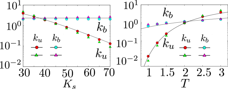
Figure 6: Dependence of binding (unbinding) rates $k_{b}$ ($k_{u}$) on (a) the strength of the particle-filament binding potential, $K_{s}$, and (b) temperature, $T$, calculated using the two different numerical methods (filled symbols) discussed in the text. These can be fit, with no undetermined parameter, to the analytic forms (solid lines) discussed in the text (Eq. 8).

III Density fluctuations of passive advective scalars in an active medium

We now study the statistics of density fluctuations and dynamics of the actively driven passive particles. We find that the active driving tends to cluster the passive particles; this shows up in the two point spatial density correlation function and the statistics of the density fluctuations.

III.1 Radial distribution function

We study the behaviour of the radial distribution function of the passive particles $g(r)$,

$$g(r)=\frac{1}{N_{p}\rho}\Bigg{\langle}\sum\limits_{i}\sum\limits_{i\neq j}\delta(r-{\lvert\bf r_{i}-r_{j}\rvert})\Bigg{\rangle},$$ (12)

where $N_{p}$ is the total number of passive particles and $\rho$ the passive particle density. When $k_{b}=0$ and $f_{0}=0$, i.e., when the particles do not bind to the filament (inert particles) and there is no propulsion force, $g(r)$ has the form of a dilute fluid (Fig. 7). When we allow for particle binding, but in the absence of propulsion force, the $g(r)$ displays oscillations, which arise from particles binding to periodic locations on the filaments (Fig. 7) - note $r=20$ coincides with the filament length. In this equilibrium situation, the particles not bound to the filaments do not show any clustering.

We now consider the case when the filaments are driven by a propulsion force $f_{0}$. We find that in addition to the periodically spaced bound particles, there is a significant fraction of unbound particles that are clustered (Fig. 7). This clustering is a consequence of the shepherding of passive particles by the active filaments - this has also been reported in nitin , with the difference that in that case the dynamics of the particles affects the active filaments.

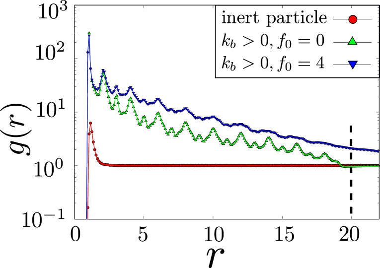
Figure 7: Radial distribution function $g(r)$ for inert particles ($k_{b}=0$ : red $\bullet$), passive particles which can bind to the filaments at equilibrium ($k_{b}>0$, $f_{0}=0$ : green $\bigtriangleup$) and passive particles which can bind to the self-propelled filaments ($k_{b}>0$, $f_{0}=4$ : blue $\bigtriangledown$). In the presence of activity the peak heights increase and $g(r)$ falls off more gradually, indicating a high degree of clustering in both the bound and unbound particles.

III.2 Probability distribution of local number density

This activity induced clustering of the passive particles should be reflected in the probability distribution of the excess number density. To compute this we divide the system into blocks of size $\Omega=39.64$ and count the number of passive particles $n$ in each block, to obtain the steady state distribution $P(n)$.

The inert particles, in the dilute limit (Fig. 8), has a probability distribution that resembles a gas at temperature $T$ and the average number of particle in the blocks $\bar{n}$, namely,

$$P(n)=\frac{1}{\sqrt{2\pi\sigma^{2}}}\exp{\left[-\frac{(n-{\bar{n}})^{2}}{2\sigma^{2}}\right]}$$ (13)

where $\bar{n}=\Omega\rho$. We have taken the variance of the above distribution to have a virial form, $\sigma^{2}=\bar{n}-\frac{2B_{2}}{\Omega}{\bar{n}}^{2}+\ldots$ - a fit to the numerical data gives $B_{2}=-0.99$ (dark line in Fig. 8).

On the other hand, the probability distribution for passive particles picks up an exponential tail arising from the binding-unbinding statistics of the particles. This exponential tail gets more pronounced when the filaments are made active, and which moves towards the typical value as the active propulsion force gets larger (Fig. 8). This reflects the fact that for high driving, the typical particle is clustered. Both these results are entirely consistent with the experimental observations reported in Fig. 4 D of darius .

III.3 Number fluctuations : crossover from anomalous to Brownian

Note that the active system of filaments is in the isotropic phase and we should not expect to see giant number fluctuations normally associated with active systems with global orientational order toner-tu ; simha ; vijay . However when we compute the root mean square fluctuations $\bigtriangleup n$ and mean ${\bar{n}}$ of the number of passive particles over regions of ever increasing area, and plot them with respect to each other, we find that initially $\bigtriangleup n\propto{\bar{n}}^{\alpha}$ with $\alpha=0.784$. Subsequently, as ${\bar{n}}$ increases, the variance scaling shows a cross over to $\alpha=0.5$. This crossover occurs over a scale corresponding to the orientational correlation length, which can in principle be large, especially close to the isotropic-nematic transition or high $f_{0}$. This is especially apparent in the high particle density regime, see Fig. 9 for particle density $\rho=0.05$ and filament density $c=0.02$. This slow crossover is consistent with the experiments on the in vitro reconstitutions of actomyosin on a supported bilayer darius .

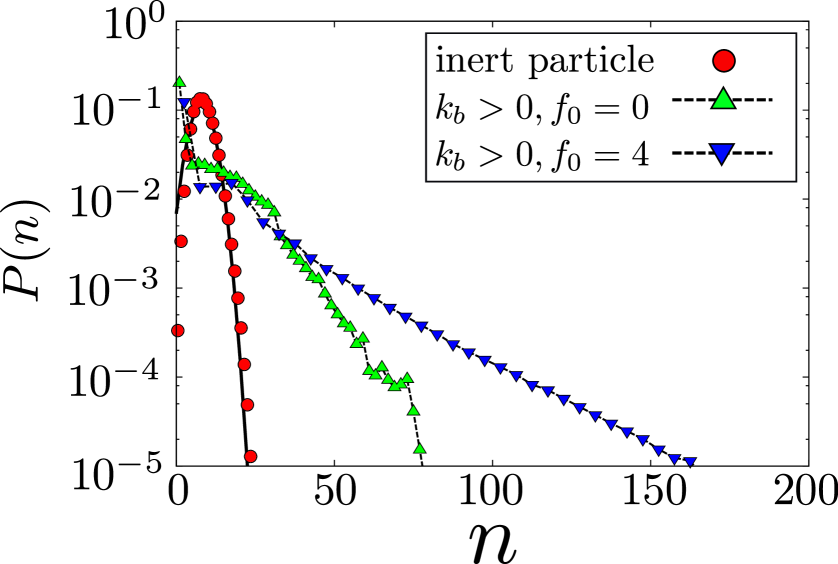
Figure 8: Probability distribution of number density $P(n)$ for inert particles ($k_{b}=0$ : red $\bullet$), passive particles which can bind to the filaments at equilibrium ($k_{b}>0$, $f_{0}=0$ : green $\bigtriangleup$) and passive particles which can bind to the self-propelled filaments ($k_{b}>0$, $f_{0}=4$ : blue $\bigtriangledown$). For inert particles, $P(n)$ fits the virial expression Eq. 13 (dark line) with a second virial coefficient, $B_{2}=-0.99$. $P(n)$ picks up an exponential tail for particles that bind and unbind onto the filaments, that moves towards the typical value as the active propulsion force gets larger.

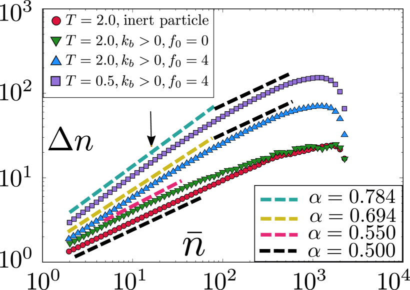
Figure 9: Root mean square fluctuations of the number of passive particles $\Delta n$ versus the mean ${\bar{n}}$ for inert (red $\bullet$) and passive particles at two different temperatures, $T=0.5$ ($\bigtriangleup$) and $T=2.0$ ($\square$). Dashed lines indicate the local slope $\alpha$ in this log-log plot of $\Delta n\propto{\bar{n}}^{\alpha}$. The values of $\alpha$ indicated in the legend, show that while inert particles exhibit normal fluctuations ($\alpha=0.5$), passive particles show large fluctuations at small ${\bar{n}}$ (with $\alpha$ depending on $T$ and $f_{0}$) that crosses over to normal fluctuations beyond a scale corresponding to the orientational correlation length (indicated by the arrow).

IV Transport of passive advective scalars in an active medium

We now study the transport of passive particles moving in the active medium. Because the filaments are orientationally disordered, the long time dynamics of the particles is always diffusive. However the diffusion characteristics can change depending on the statistics of (un)binding to the active filaments.

IV.1 Typical trajectories

The space-time trajectories of the passive particles show three qualitatively different behaviours. At very low temperatures compared to ${\overline{U}}=K_{s}r_{0}^{2}/4$, a passive particle once bound to a filament, rarely unbinds, and hence gets advected with the self-propelled filament (Fig. 10(a)).

The direction of advection changes because of thermal fluctuations and collisions between filaments.

Figure 10: Typical trajectories of passive particles for a fixed propulsion force $f_{0}=4.0$ at different temperatures - (a) $T=0.5$ (low : $k_{B}T/{\overline{U}}=0.04$); (b) $T=4.0$ (intermediate : $k_{B}T/{\overline{U}}=0.32$) and (c) $T=10.0$ (high : $k_{B}T/{\overline{U}}=0.8$).

Increasing the temperature increases the probability of unbinding from the filament, whereupon the particle undergoes unrestricted thermal diffusion before binding again (Fig. 10(b)). At even higher temperatures, $k_{B}T/{\overline{U}}\approx 1$ the particles do not bind to the filaments and the motion is simple thermal diffusion (Fig. 10(c)).

IV.2 Statistics of displacements and diffusion coefficient

Propensity distribution. The distribution of displacements $\Delta x$ (along the ${\hat{\bf x}}$ direction) evaluated over a time window $t_{w}$ is called the propensity distribution. This will depend on the statistics of binding/unbinding, which in turn depends on the temperature $T$ and $f_{0}$, densities of filaments and particles, and of course on the time window $t_{w}$, which we fix at $t_{w}=10$. This can be obtained both from our Brownian dynamics simulation and, in the dilute limit, analytically.

In the dilute limit, one can obtain the form of this probability distribution from the stationary process describing the particle vector-displacements in a small time interval $t_{w}$,

$${\bf r}(t_{w})={\bf r}(0)+\int_{0}^{t_{w}}{\bf V}(t^{\prime})\,dt^{\prime}$$ (14)

where ${\bf V}$ is the velocity of the tagged particle at time $t$, given by,

$${\bf V}(t)=\phi(t)\,\frac{f_{0}}{\gamma}\,{\bf{\hat{n}}}(t)+(1-\phi(t))\,{\bm{\xi}}(t),$$ (15)

where $\bf{\hat{n}}$ is the polar vector representing the orientation of the filament to which the particle is bound at time $t$, ${\bm{\xi}}$ is the thermal noise, and $\phi(t)$ is the telegraphic noise whose statistics is described in Sect. II D. The distribution of the particle displacements $\Delta x_{t_{w}}\equiv\left({\bf r}(t_{w})-{\bf r}(0)\right)\cdot{\hat{\bf x}}$, can be obtained by evaluating,

$$P(\Delta x)=\langle\delta\left(\Delta x-\Delta x_{t_{w}}\right)\rangle$$ (16)

where $\Delta x_{t_{w}}$ is obtained from Eq. 14 and the angular bracket denotes an average over the joint distribution of $\bm{\xi}$ and $\phi$. This can be evaluated by standard techniques of Fourier transformation and cumulant expansion kampen ,

$$\ln{\tilde{P}}(k)=\sum_{m=1}^{\infty}\frac{(ik)^{m}}{m!}\langle\left(\Delta x_{t_{w}}\right)^{m}\rangle_{c}$$ (17)

where ${\tilde{P}}(k)$ is the Fourier transform of $P(\Delta x)$. The $m$-th cumulants $\langle\left(\Delta x_{t_{w}}\right)^{m}\rangle_{c}$ can be evaluated from Eqs. 14, 15, knowing that $\phi$ and ${\bm{\xi}}$ are independent stochastic processes. The distribution $P(\Delta x)$ is then obtained by taking the inverse Fourier transform of ${\tilde{P}}(k)$.

However, in practice, the inverse Fourier transform of ${\tilde{P}}(k)$, for the stationary process Eq. 14, has to be evaluated numerically. Rather than do this, we provide an alternate argument which gives more insight.

At low enough $T$, the passive particles are completely bound to the self-propelled filaments, and so as long as $t_{w}<\tau$, the orientational correlation time of the filaments, the particles get displaced by $\Delta{\bf{r}}=\frac{f_{0}t_{w}}{\gamma_{p}}\bf{\hat{n}}$, where $\gamma_{p}$ is the friction coefficient and $\bf{\hat{n}}$ is the unit vector representing the average orientation of a filament during time interval $t_{w}$. Since the filament orientation is uniformly distributed, the contribution to the step-size distribution from this process is $P(\Delta x)=\frac{\gamma_{p}}{\pi f_{0}t_{w}}\frac{1}{\sqrt{1-(\frac{\gamma_{p}}{f_{0}}\frac{\Delta x}{t_{w}})^{2}}}$. On the other hand, at very high $T$, the particles are completely unbound and undergo thermal diffusion, for which the step-size distribution is $P({\Delta x})=\frac{1}{\sqrt{2\pi\sigma^{2}}}\exp{[-\frac{(\Delta x)^{2}}{2\sigma^{2}}]}$, where $\sigma^{2}=\frac{2k_{B}T}{\gamma_{p}}t_{w}$. We propose that at an intermediate $T$, the propensity distribution can be written as a linear combination, weighted by the duty ratio $\langle\phi\rangle$, i.e.,

$$P(\Delta x)=\frac{\gamma_{p}}{\pi f_{0}t_{w}}\frac{\langle\phi\rangle}{\sqrt{1-\left(\frac{\gamma_{p}}{f_{0}}\frac{\Delta x}{t_{w}}\right)^{2}}}+$$

$$\frac{1-\langle\phi\rangle}{\sqrt{2\pi\sigma^{2}}}\exp{\left[-\frac{(\Delta x)^{2}}{2\sigma^{2}}\right]}.$$ (18)

The agreement of this approximate analytical form, with no undetermined parameters, with the results of the Brownian simulation is quite reasonable, see Fig. 11.

Figure 11: Probability distribution $P(\Delta x)$ of the displacements of passive particles, evaluated for fixed time interval $\bigtriangleup t=10$, at a propulsion force $f_{0}=4.0$ and temperatures (a) $T=0.5$ and (b) $T=2.0$. The central peak comes from the fraction undergoing thermal diffusion, while the side peaks come from the bound fraction undergoing active motion. The black filled line shows parameter-free fits to the approximate analytical form (Eq. 18), where we have estimated the value of $\langle\phi\rangle=0.9995$ at $T=0.5$ (mainly bound) and $\langle\phi\rangle=0.632$ at $T=2.0$.

Mean square displacement. From the statistics of the displacement we can compute the mean square displacement (MSD) as $\langle\Delta{\bf r}^{2}(t)\rangle=\langle\frac{1}{N_{p}}\sum_{i}|{\bf r}_{i}(t_{0}+t)-{\bf r}_{i}(t_{0})|^{2}\rangle$, where ${\bf r_{i}}$ is the position of $i$-th particle. This shows a change from a short time diffusive regime crossing over to a long time diffusive regime via an intermediate super-diffusive regime (Fig. 12(a)). We estimate the second crossover time $t_{c}(T,f_{0})$ from the super-diffusive to late time diffusion $D$, by fitting the simulation data to $\langle\Delta{\bf r}^{2}(t)\rangle=4Dt\,[1-\exp(-t/t_{c})]$ libchaber , using which we can collapse the MSD data for different values of active propulsion $f_{0}$ (Fig. 12(b)). From this we see that $t_{c}$ decreases with $f_{0}$ (Fig. 12(b) inset). This is because the filament orientation decorrelates on account of collisions, whose frequency increases with $f_{0}$. In experimental systems where hydrodynamics plays a crucial role libchaber , this dependence of $t_{c}$ on $f_{0}$ may be different.

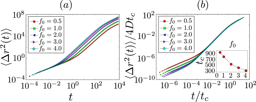
Figure 12: (a) MSD of passive particles as a function of time at $T=0.5$ for different values of self-propulsion force $(f_{0})$ of the filaments. (b) Collapse of MSD using crossover time ($t_{c}$) and long time diffusion constant for the same case. Inset shows crossover time $(t_{c})$ as a function of self-propulsion force $(f_{0})$ of the active filaments for the same case.

In situations where the crossover $t_{c}$ is large, the apparent super-diffusion behaviour would last for many decades in time. We can then fit the MSD to $\langle\Delta{\bf r}^{2}(t)\rangle\sim t^{\beta}$ to obtain an super-diffusion exponent $\beta>1$ - we find that $\beta=1.95$ at $T=0.5$ and $\beta=1.77$ at $T=2.0$, for a propulsion force $f_{0}=4.0$.

Temperature and activity dependence of MSD. We now compute the late time diffusion coefficient of the tagged particles, $D=\lim_{t\to\infty}\langle\Delta{\bf r}^{2}(t)\rangle/4t$, for different $T$ and $f_{0}$. For a fixed $f_{0}$, one might expect that at low temperatures $D$ is weakly dependent on (or even independent of) temperature because a particle once bound to the filament remains so and undergoes active diffusion as it is transported by the filament (Fig. 13). As we increase the temperature, $D$ decreases, since a particle spends less time, on an average, bound to the filament (recall we have set $\gamma_{b}=\gamma_{p}$). At high temperatures, the particles are predominantly unbound, and hence $D$ resembles that of an inert particle, which increases linearly with temperature. This is indeed what we see from a direct numerical simulation of the Brownian dynamics trajectories of a tagged particle (Fig. 13).

Figure 13: (a) Diffusion coefficient ($D$) of tagged passive particles has been plotted as a function of $T$ for different values of $f_{0}$ of the filaments. At low temperature regime $D$ is weakly dependent on $T$ (signature of ‘active diffusion’). At intermediate regime $D$ decreases then again increases at high temperature regime where thermal diffusion dominates. (b) We have plotted total diffusion coefficient $D$ (with points) and active diffusion coefficient $D_{a}$ ( with line) with $f_{0}$ for different $T$. In low temperature and high activity regime the difference between $D$ and $D_{a}$ is insignificant, as we increase $T$ and decrease $f_{0}$ the difference becomes prominent.

From the stationary process, Eq. (14), the MSD of the tagged passive particle,

$$\langle\delta{\bf r}^{2}(t)\rangle=\,\int_{0}^{t}\int_{0}^{t}\langle{\bf V}(t^{\prime})\cdot{\bf V}(t^{\prime\prime})\rangle dt^{\prime}dt^{\prime\prime}\,,$$ (19)

immediately gives the diffusion coefficient,

$$D=\frac{1}{2}\int^{\infty}_{0}\langle{\bf V}(t)\cdot{\bf V}(0)\rangle dt.$$ (20)

Using Eq. (15), we see that the diffusion coefficient of the bound particle is given by the correlations of ${\bf V}_{a}$, which is given by (Fig. 14(a)),

$$\langle{\bf V}_{a}(t)\cdot{\bf V}_{a}(0)\rangle = \frac{f_{0}^{2}}{\gamma_{p}}\langle\cos(\theta(t)-\theta(0))\rangle$$ (21)

$$= \frac{f_{0}^{2}}{\gamma_{p}}e^{-\,\mid t\mid/\tau}$$

The diffusion coefficient can now be simply evaluated,

$$D=\frac{f_{0}^{2}\tau k_{b}(\tau k_{b}+1)}{2\gamma_{p}^{2}(k_{u}+k_{b})[(k_{u}+k_{b})\tau+1]}+\frac{k_{B}Tk_{u}}{\gamma_{p}(k_{u}+k_{b})}$$ (22)

To plot $D$ versus $T$ and $f_{0}$, we need to know the values of $k_{b}$, $k_{u}$ (equivalently $\langle\phi\rangle$, $t_{sw}$) and $\tau$, which depend on the temperature and density, and which we obtain from our simulations. We then compare this semi-analytical form to the direct numerical computation of the diffusion coefficient from the Brownian dynamics trajectories (Fig. 14). The agreement between the two is excellent. These observations are entirely consistent with the results of saha .

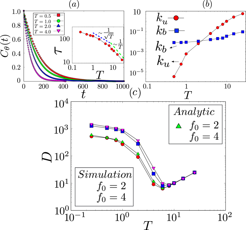
Figure 14: (a) Temporal correlation of the direction of persistent movement of the filaments, measured by the velocity orientation correlation function $C_{\theta}(t)$, at different temperatures, with the filament density $c=0.01$ and propulsion force $f_{0}=4$. Inset shows the corresponding orientation correlation time $\tau$ as a function of $T$. (b) Temperature dependence of binding ($k_{b}$) and unbinding ($k_{u}$) rates calculated from the statistics of the telegraphic noise $\phi(t)$. (c) Both, simulation and analytic calculation of diffusion coefficient ($D$) of tagged passive particles has been plotted as a function of temperature ($T$) for two different activities ($f_{0}=2,4$) for filament density $c=0.01$.

It might be objected that in our analysis we have treated the active propulsion as an independently tunable parameter, thus precluding the possibility that the activity itself may be temperature dependent. However, as we saw in Goswami , and as noted elsewhere spudich ; levy , the actomyosin contractile processes taken as a whole, appear to be independent of temperature in the physiological range, $24^{\circ}-37^{\circ}$C.

Figure 15 shows the dependence of $D$ on filament concentration $c$, both from direct simulations and from the analytical form using the values of $k_{b}$, $k_{u}$ (equivalently $\langle\phi\rangle$, $t_{sw}$) and $\tau$, from simulations. This shows optimal transport at a specific filament concentration; the orientational decorrelation time is smaller at higher filament concentration, due to higher collision frequency.

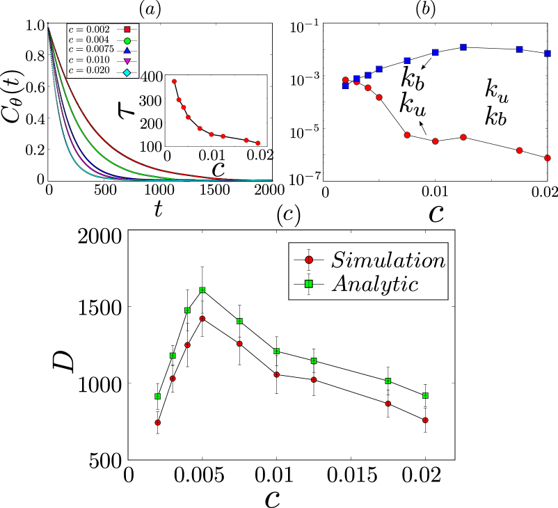
Figure 15: (a) Temporal correlation of the direction of persistent movement of the filaments, measured by the velocity orientation correlation function $C_{\theta}(t)$, with different filament density ($c$), at temperature $T=0.5$ and propulsion force $f_{0}=4$. Inset shows the corresponding orientation correlation time $\tau$ as a function of $c$. (b) Dependence of binding ($k_{b}$) and unbinding ($k_{u}$) rates on filament density $c$, calculated form the statistics of the telegraphic noise $\phi(t)$. (c) Both, simulation and analytic calculation of diffusion coefficient ($D$) of tagged passive particles has been plotted as a function of filament density ($c$) at $T=0.5$ and for $f_{0}=4$.

V Viscosity stratification and its effect on membrane diffusion

So far, our study of transport of passive molecules in an active medium has been restricted to two dimensions. However as we discussed in Sect. I, the cell surface is a composite of a bilayer membrane and a thin actomyosin cortex. Thus while the proteins move on the cell membrane, the actively driven actin moves in the actomyosin cortex. The viscosities of these two layers are significantly different, with the bilayer membrane having a viscosity which is an order of magnitude larger than the cortex ($\approx 0.86$ Pa s kamm ). Indeed the local viscosity of a multicomponent membrane can be quite heterogeneous - for instance the particle mobility within the so-called “membrane rafts” or liquid-ordered regions on the cell membrane can be very different from those within liquid-disordered regions. Moreover the local cortical viscosity depends on local actin, myosin and cross-linker concentrations. How does this viscosity mismatch affect the actively driven transport of passive molecules?

To address this important issue within our simulation, we vary the ratio of the friction coefficients $\Gamma=\gamma_{p}/\gamma_{b}$ in Eqs. 3, 4. We find that the mean fraction of passive particles bound to filaments $\langle n_{b}\rangle$ decreases with increasing $\Gamma$ over a range of $T$ and $f_{0}=4.0$ (Fig. 16(a)). This is an interesting observation, since one might have naively thought that $\langle n_{b}\rangle$ is solely governed by binding-unbinding, a purely equilibrium process and hence independent of relative viscosities. However, we see that the drag induced by the imposed viscosity stratification (a nonequilibrium feature), can “peel-off” particles from the filaments. It is not clear to us why we see a shoulder at intermediate values of $\Gamma$ for low enough temperatures (Fig. 16(a)).

This is reflected in changes that we observe in the measured diffusion coefficient $D$, as it decreases with increasing $\Gamma$ at different $T$ (Fig. 16(b)). As can be seen, the active-diffusion regime at low temperatures becomes significantly more temperature dependent as the viscosity mismatch $\Gamma$ increases.

The results of this section are not purely academic, on the contrary taken together they pose an interesting possibility that by tuning local viscosity mismatch, for instance by locally recruiting the so-called “membrane rafts” or liquid-ordered regions on the cell membrane or by locally regulating the concentrations of actin, myosin or cross-linkers, the living cell surface could control the clustering and transport of specific membrane proteins.

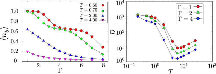
Figure 16: (a) Fraction of bound particles $\langle n_{b}\rangle$ decreases with $\Gamma=\gamma_{p}/\gamma_{b}$ over a range of temperatures. (b) Diffusion coefficient versus temperature at different values of viscosity mismatch parameter $\Gamma$. In both figures, the propulsion force has been fixed at $f_{0}=4.0$.

VI Discussion

We had earlier shown that a coarse grained active hydrodynamics description of the active composite cell surface, successfully explains the statistics of clustering of membrane proteins capable of binding to the cortical actomyosin in living cells raomayor ; kripa . Such a description make predictions regarding the statistics of density fluctuations and transport of such actin-binding membrane proteins, which were verified in experiments kripa ; saha . Following this we were able to recapitulate much of this behaviour in a minimal in vitro system comprising a thin layer of short actin filaments and Myosin-II minifilaments on a supported bilayer darius . The success of this approach has motivated us to do a agent-based Brownian dynamics simulation using these minimal ingredients - that of a collection of passive molecules which bind/unbind to actin filaments and move in this active medium in two dimensions.

The results obtained here, based on simulations and analytical calculations, are in qualitative agreement with the experiments both in vivo and in vitro. For instance, the exponential tails appearing in the probability distribution of the number (Fig. 8) and the scaling of the variance of the number (Fig. 9) is precisely the behaviour seen in our earlier in vitro experiments. In addition, we show how activity induced clustering of passive particles (Fig. 7) arises naturally from such a minimal description.

We have also studied transport of passive particles moving in this active medium, and find that there is a crossover from an intermediate time super diffusive to late time diffusive behaviour as a consequence of active driving (Fig. 12(a)). The transport behaviour shows a striking dependence on temperature and active forcing - at low temperatures the diffusion coefficient is insensitive to temperature, and crosses over to a linear temperature dependence at higher temperatures, in qualitative agreement with experiments saha .

Finally, recognising that the viscosity of the cortical layer is different from that of the membrane, we show that a friction coefficient mismatch has a strong effect on the mean number of bound particles and the diffusion coefficient. This is a consequence of the drag induced by the imposed viscosity stratification, which results in a “peeling-off” of the particles from the filaments. This opens up the possibility of local tuning of viscosity mismatch, for instance by locally recruiting the so-called “membrane rafts” or liquid-ordered regions on the cell membrane or by locally regulating the concentrations of actin, myosin or cross-linkers. This could result in yet another mechanism by the cell surface might locally control the clustering and transport of specific membrane proteins. We hope that some of these predictions can be tested in future experiments.

VII Acknowledgement

We thank K. Husain, R. Morris and D. Banerjee for critical inputs. MR thanks S. Mayor and D. Koster for long years of collaboration. SKRH and RM thank the Simons Centre at NCBS for computational facilities and hospitality. RM acknowledges financial support from CSIR, India.

References

- (1) M. Rao and S. Mayor, Curr. Op. Cell Biol. 29, 126 (2014).
- (2) D. Goswami et al., Cell 135, 18085 (2008).
- (3) K. Gowrishankar, S. Ghosh, S. Saha, S. Mayor and M. Rao, Cell 149, 1353 (2012).
- (4) S. Saha, I. Lee, A. Polley, J. T. Groves, M. Rao and S. Mayor, Mol. Biol. Cell 26, 4033 (2015).
- (5) S.J. Plowman, C. Muncke, R.G. Parton and J.F. Hancock, Proc. Natl. Acad. Sci. USA 102, 15500 (2005).
- (6) D. Lingwood and K. Simons, Science 327, 46 (2010).
- (7) P. Chugh, A.G. Clark, M. B. Smith, D. A. D. Cassani, K. Dierkes, A. Ragab, P. P. Roux, G. Charras, G. Salbreux and E. K. Paluch, Nat. Cell Biol. 19, 697 (2017).
- (8) Morone et al., J. Cell Biol., 174, 851 (2006).
- (9) K. Gowrishankar and M. Rao, Soft Matter 12, 2040-2046 (2016).
- (10) M. C. Marchetti, J. F. Joanny, S. Ramaswamy, T. B. Liverpool, J. Prost, M. Rao and R. A. Simha, Rev. Mod. Phys. 85, 1143 (2013).
- (11) D.V. Koster, K. Husain, E. Iljazi, A. Bhat, P. Bieling, R.D. Mullins, M. Rao and S. Mayor, Proc. Natl. Acad. Sci. USA 113, E1645 (2016).
- (12) T. Fujiwara, K. Ritchie, H. Murakoshi, K. Jacobson and A. Kusumi, J. Cell Biol. 157, 904 (2002).
- (13) Y. Hatwalne, S. Ramaswamy, M. Rao, and R. A. Simha, Phys. Rev. Lett. 92, 118101 (2004).
- (14) A. Basu, J. F. Joanny, F. Julicher, and J. Prost, New J. Phys. 14, 115001 (2012).
- (15) K. Chen, B. Wang, and S. Granick, Nat. Mater. 14, 589 (2015).
- (16) T. C. Bidone, W. Jung, D. Maruri, C. Borau, R. D. Kamm and T. Kim, PLoS Comput Biol 13, 1005277 (2017).
- (17) D. Grebenkov, J. Phys. A 48, 013001 (2015).
- (18) N.G. Van Kampen in Stochastic Processes in Physics and Chemistry, 3rd Edition, North-Holland, Amsterdam (2007).
- (19) N. Kumar, H. Soni, S. Ramaswamy and A. K. Sood, Nat. Comm. 5, 4688 (2014).
- (20) J. Toner and Y. Tu, Phys. Rev. Lett. 75, 4326 (1995).
- (21) V. Narayan, S. Ramaswamy and N. Menon, Science 317, 105 (2007).
- (22) R. A. Simha, J. Toner and S. Ramaswamy, EPL 62, 2 (2003).
- (23) X. Wu and A. Libchaber, Phys. Rev. Lett. 84, 3017 (2000).
- (24) M. P. Sheetz, R. Chasan and J. A. Spudich, J. Cell Biol. 99, 1867 -1871 (1984).
- (25) H.M. Levy, N. Sharon, and D. E. Koshland Jr., Proc. Natl. Acad. Sci. USA 45, 785- 791 (1959).