A Spectral Element Reduced Basis Method in Parametric CFD

Abstract

We consider the Navier-Stokes equations in a channel with varying Reynolds numbers. The model is discretized with high-order spectral element ansatz functions, resulting in $14^{\prime}259$ degrees of freedom. The steady-state snapshot solutions define a reduced order space, which allows to accurately evaluate the steady-state solutions for varying Reynolds number with a reduced order model within a fixed-point iteration. In particular, we compare different aspects of implementing the reduced order model with respect to the use of a spectral element discretization. It is shown, how a multilevel static condensation [1] in the pressure and velocity boundary degrees of freedom can be combined with a reduced order modelling approach to enhance computational times in parametric many-query scenarios.

1 Introduction

The use of spectral element methods in computational fluid dynamics [1] allows highly accurate computations by using high-order spectral element ansatz functions. Typically, an exponential error decay can be observed under p-refinement. See [2], [3], [4], [5], [6] for an introduction and overview of the applications.

This work is concerned with the reduced basis method (RBM, [7]) of a channel flow, governed by the Navier-Stokes equations, and discretized with the spectral element method into $14^{\prime}259$ degrees of freedom. In particular, we are interested in computing the steady-state solutions for varying Reynolds number with a reduced order model, guaranteeing competitive computational performances.

Section 2 introduces the governing equations and used fixed-point iteration algorithm. Section 3 introduces the spectral element discretization, while section 4 describes the model reduction approach. Numerical results are provided in section 5, while section 6 summarizes and concludes the work by also providing new perspectives.

2 Problem Formulation

Let $\Omega\in\mathbb{R}^{2}$ be the computational domain. Incompressible, viscous fluid motion in a spatial domain $\Omega$ over a time interval $(0,T)$ is governed by the incompressible Navier-Stokes equations with velocity $\mathbf{u}$, pressure $p$, kinematic viscosity $\nu$ and a body forcing $f$, (1) - (2):

$$\frac{\partial\mathbf{u}}{\partial t}+\mathbf{u}\cdot\nabla\mathbf{u} = -\nabla p+\nu\Delta\mathbf{u}+f,$$ (1)

$$\nabla\cdot\mathbf{u} = 0.$$ (2)

Boundary and initial conditions are prescribed as

$$\mathbf{u} = d\quad\text{ on }\Gamma_{D}\times(0,T),$$ (3)

$$\nabla\mathbf{u}\cdot n = g\quad\text{ on }\Gamma_{N}\times(0,T),$$ (4)

$$\mathbf{u} = u_{0}\quad\text{ in }\Omega\times 0,$$ (5)

with $d$, $g$ and $u_{0}$ given and $\partial\Omega=\Gamma_{D}\cup\Gamma_{N}$, $\Gamma_{D}\cap\Gamma_{N}=\emptyset$. The Reynolds number $Re$ depends on the viscosity $\nu$ through the characteristic velocity $U$ and characteristic length $L$ via $Re=\frac{UL}{\nu}$, [12].

In particular, we are interested in computing the steady states for varying viscosity $\nu$, such that $\frac{\partial\mathbf{u}}{\partial t}=0$. A solution $\mathbf{u}(\nu_{1})$ for a parameter value $\nu_{1}$, can be used as an initial guess for a fixed point iteration to obtain the steady state solution $\mathbf{u}(\nu_{2})$ at a parameter value $\nu_{2}$, provided that the solution $\mathbf{u}(\nu)$ depends continuously on $\nu$ in the interval $[\nu_{1},\nu_{2}]$.

2.1 Oseen-Iteration

The Oseen-iteration is a secant modulus fixed-point iteration, which in general exhibits a linear rate of convergence [8]. Given a current iterate (or initial condition) $\mathbf{u}^{k}$, the linear system

$$-\nu\Delta\mathbf{u}+(\mathbf{u}^{k}\cdot\nabla)\mathbf{u}+\nabla p = f\text{ in }\Omega,$$ (6)

$$\nabla\cdot\mathbf{u} = 0\text{ in }\Omega,$$ (7)

$$\mathbf{u} = d\quad\text{ on }\Gamma_{D},$$ (8)

$$\nabla\mathbf{u}\cdot n = g\quad\text{ on }\Gamma_{N},$$ (9)

is solved for the next iterate $\mathbf{u}^{k+1}=\mathbf{u}$. A typical stopping criterion is that the relative change between iterates in the $H^{1}$ norm falls below a predefined tolerance. An initial solution $\mathbf{u}^{0}(\nu_{0})$ is computed by time-advancement of (1)–(2) from zero initial conditions at a parameter value $\nu_{0}$, and the whole parameter domain is then explored by using a continuation method with the Oseen-iteration.

3 Spectral Element Discretization

The Navier-Stokes problem is discretized with the spectral element method. The spectral/hp element software framework used is Nektar++ in version 4.3.5, [9]. The discretized system to solve in each step of the Oseen-iteration is given by (10) as

$$\begin{bmatrix}\begin{array}[]{ccc}A&-D^{T}_{bnd}&B\\ -D_{bnd}&0&-D_{int}\\ \tilde{B}^{T}&-D^{T}_{int}&C\end{array}\end{bmatrix}\begin{bmatrix}\begin{array}[]{ccc}v_{bnd}\\ p\\ v_{int}\end{array}\end{bmatrix} =\begin{bmatrix}\begin{array}[]{ccc}f_{bnd}\\ 0\\ f_{int}\end{array}\end{bmatrix},$$ (10)

where $v_{bnd}$ and $v_{int}$ denote velocity degrees of freedom on the boundary and in the interior, respectively. Correspondingly, $f_{bnd}$ and $f_{int}$ denote forcing terms on the boundary and interior, respectively. The matrix $A$ assembles the boundary-boundary coupling, $B$ the boundary-interior coupling, $\tilde{B}$ the interior-boundary coupling and $C$ assembles the interior-interior coupling of elemental velocity ansatz functions. In the case of a Stokes system, it holds that $B=\tilde{B}^{T}$, but this is not the case for the Oseen equation, since the linearization term $(\mathbf{u}^{k}\cdot\nabla)\mathbf{u}$ is present in (6). The matrices $D_{bnd}$ and $D_{int}$ assemble the pressure-velocity boundary and pressure-velocity interior contributions, respectively.

The linear system (10) is assembled in local degrees of freedom, resulting in block matrices $A,B,\tilde{B},C,D_{bnd}$ and $D_{int}$, each block corresponding to a spectral element. In particular, this means that the system is singular in this form. To solve the system, the local degrees of freedom need to be gathered into the global degrees of freedom [1]. Since $C$ contains the interior-interior contributions, it is invertible and the system can be statically condensed into

$$\begin{bmatrix}\begin{array}[]{ccc}A-BC^{-1}\tilde{B}^{T}&BC^{-1}D^{T}_{int}-D^{T}_{bnd}&0\\ D_{int}C^{-1}\tilde{B}^{T}-D_{bnd}&-D_{int}C^{-1}D^{T}_{int}&0\\ \tilde{B}^{T}&-D^{T}_{int}&C\end{array}\end{bmatrix} \begin{bmatrix}\begin{array}[]{ccc}v_{bnd}\\ p\\ v_{int}\end{array}\end{bmatrix}$$

$$= \begin{bmatrix}\begin{array}[]{ccc}f_{bnd}-BC^{-1}f_{int}\\ D_{int}C^{-1}f_{int}\\ f_{int}\end{array}\end{bmatrix}.$$ (11)

By taking the top left $2\times 2$ block and reordering the degrees of freedom such that the mean pressure mode of each element is inserted into the corresponding block of $\hat{A}$ results in

$$\begin{bmatrix}\begin{array}[]{cc}\hat{A}&\hat{B}\\ \hat{C}&\hat{D}\end{array}\end{bmatrix}\begin{bmatrix}\begin{array}[]{ccc}b\\ \hat{p}\end{array}\end{bmatrix} =\begin{bmatrix}\begin{array}[]{ccc}\hat{f}_{bnd}\\ \hat{f}_{p}\end{array}\end{bmatrix},$$ (12)

where $\hat{D}$ is invertible, such that a second level of static condensation can be employed. We have:

$$\begin{bmatrix}\begin{array}[]{cc}\hat{A}-\hat{B}\hat{D}^{-1}\hat{C}&0\\ \hat{C}&\hat{D}\end{array}\end{bmatrix}\begin{bmatrix}\begin{array}[]{ccc}b\\ \hat{p}\end{array}\end{bmatrix} =\begin{bmatrix}\begin{array}[]{ccc}\hat{f}_{bnd}-\hat{B}\hat{D}^{-1}\hat{f}_{p}\\ \hat{f}_{p}\end{array}\end{bmatrix}.$$ (13)

When the vector $b$ is computed, which contains the velocity boundary degrees of freedom and the mean pressure modes, the remaining solution components are computed by reverting the steps of the static condensations [1]. The main computational effort lies in solving the final system (14)

$$(\hat{A}-\hat{B}\hat{D}^{-1}\hat{C})b=\hat{f}_{bnd}-\hat{B}\hat{D}^{-1}\hat{f}_{p}.$$ (14)

Additionally, the matrices $C$ and $\hat{D}$ need to be inverted, which due to the elemental block structure requires inverting submatrices in the size of the degrees of freedom per element for each submatrix.

4 Reduced Order Modelling

The reduced order model (ROM) aims to represent the full order solution accurately in the parameter domain of interest. Two ingredients are essential to RB modelling, a projection onto a low order space of snapshot solutions and an offline-online decomposition for computational efficiency, [16]. A set of snapshots is generated by solving (14) over a coarse discretization of the parameter domain and used to define a projection space $U$ of size $N$. The proper orthogonal decomposition computes a singular value decomposition of the snapshot solutions to $99.9\%$ of the most dominant modes [7], which defines the projection matrix $U\in\mathbb{R}^{N_{\delta}\times N}$ to project system (14) and obtain the reduced order solution $b_{N}$.

4.1 Offline-Online Decomposition

The offline-online decomposition [7] allows fast input-output evaluations independent of the original model size $N_{\delta}$. It is a crucial part of an efficient reduced order model but since the static condensation includes the inversion of the parameter-dependent matrix $C$, an intermediate projection is introduced.

The reduced order model considers the top left $2\times 2$ block of (11), i.e., one level of static condensation [1]. During the offline phase, full-order solutions have been computed over the parameter domain of interest, which now serve as a projection space to define the reduced order setting. This projection space incorporates the transformation of local velocity boundary degrees of freedom to global velocity boundary degrees of freedom and the reordering of mean pressure degrees of freedom. The projection space then takes the form $U=PMV$ with a permutation matrix $P$ to reorder the degrees of freedom and a transformation $M$ from local to global degrees of freedom. The collected offline data $V$ contain the gathered velocity and mean pressure modes as well as interior pressure modes.

The projected system is then of the form

$$A_{N}=U^{T}\begin{bmatrix}\begin{array}[]{cc}A-BC^{-1}\tilde{B}^{T}&BC^{-1}D^{T}_{int}-D^{T}_{bnd}\\ D_{int}C^{-1}\tilde{B}^{T}-D_{bnd}&-D_{int}C^{-1}D^{T}_{int}\end{array}\end{bmatrix}U,$$ (15)

and upon its solution, the interior velocity dofs can be computed by resubstituting into (11) at the reduced order level. To achieve fast reduced order solves, the offline-online decomposition expands (15) in the parameter of interest and computes the parameter independent projections offline to be stored as small-sized matrices of the order $N\times N$. Since in an Oseen-iteration each matrix is dependent on the previous iterate, the submatrices corresponding to each basis function is assembled and then formed online using the reduced basis coordinate representation of the current iterate. This is analogous to reduced order assembly of the nonlinear term in the Navier-Stokes case, [16].

5 Model and Numerical Results

We consider a channel flow in the domain considered in Fig. 1, similar to the model considered in [13]. The rectangular domain $\Omega(x,y)=[0,36]\times[0,6]$ is decomposed into $32$ spectral elements. The spectral element expansion uses modal Legendre polynomials of order $p=12$ in the velocity. The pressure ansatz space is chosen of order $p-2$ to fulfill the inf-sup stability condition, [10], [11]. The inflow is defined for $y\in[2.5,3.5]$ as $u_{x}(0,y)=(y-2.5)(3.5-y)$. At $x=36$ is the outflow boundary, everywhere else are zero velocity walls. Note that the velocity boundary degrees of freedom are along the boundaries of the spectral elements and not only the domain boundary, resulting in $3072$ local degrees of freedom for this problem.

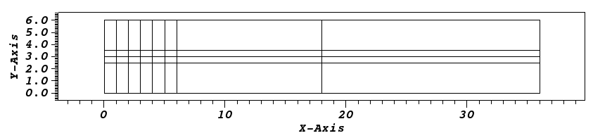
Figure 1: Rectangular domain for the channel flow, shown is the $4\times 8$ spectral element grid.

This is a simplified model of a contraction-expansion channel [12], where flow occurs though a narrowing of variable width. Variations in the width have been moved to variations in the Reynolds number and only the section after the narrowing comprises the computational domain. The relation to the Reynolds number is established with $U=\frac{1}{4}$ as the maximum inflow velocity and $L=1$ as the width of the narrowing as $Re=\frac{1}{4\nu}$.

Consider a parametric variation in the viscosity $\nu$, ranging from $\nu=0.0075$ to $\nu=0.0025$, which corresponds to Reynolds numbers between $33$ and $100$. The solution for $\nu=0.0075$ is shown in Fig. 2. It is slightly unsymmetrical, which marks the onset of the Coanda effect [14], [15], which is a known phenomenon characterized as a ‘wall-hugging’ effect occurring at these Reynolds numbers. The solution for $\nu=0.0025$ is shown in Fig. 3. Here, the Coanda effect is fully developed as the flow orients itself along the boundaries.

   
   

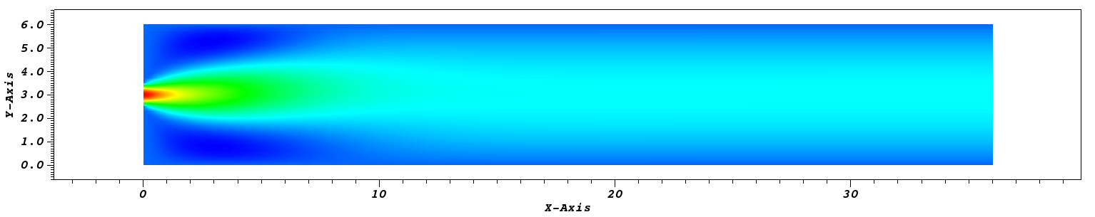
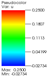
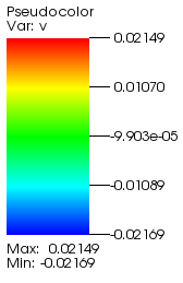
Figure 2: Full order, steady-state solution for $\nu=0.0075$. Top is the velocity in x-direction, below is the velocity in y-direction.

   
   

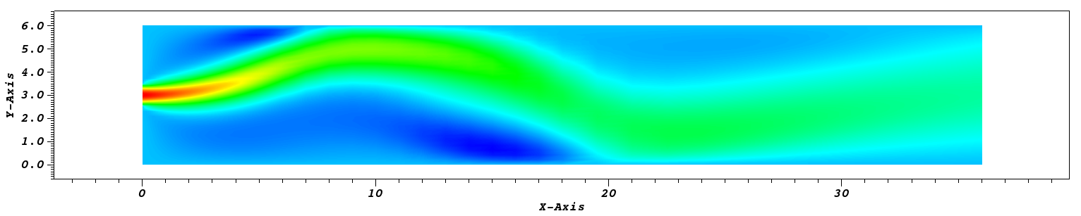
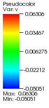
Figure 3: Full order, steady-state solution for $\nu=0.0025$. Top is the velocity in x-direction, below is the velocity in y-direction.

Using model reduction with the form (11), which allows the offline-online decomposition or using form (14), which has the lowest full-order system size, resulted in similar computational results. Shown in Fig. 4 is the relative $H^{1}_{0}(\Omega)$ error in the velocity between the full order and reduced order model.

While the full-order solves were computed with Nektar++, the reduced-order computations were done in a separate python code. To compare computational gains, compute times between a full order solve and a reduced order solve both implemented in python are taken. The compute times reduce by a factor of $50$, i.e., for a single iteration step from about $40$s to under $1$s. Current work also aims to extend the software to make it available as a SEM-ROM software framework within the AROMA-CFD project (see Acknowledgment) as ITHACA-SEM.

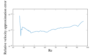
Figure 4: Relative error in the velocity over the parameter domain.

6 Conclusion and Outlook

It has been shown that the reduced basis technique generates accurate reduced order models of small size for channel flow discretized with spectral elements up to a Reynolds number of $100$. The use of basis functions obtained by the spectral element method suggests a potential important synergy between high-order and reduced basis methods, see also [6]. Due to the multilevel static condensation used here, particular care must be taken to achieve an offline-online decomposition. The domain decomposition into spectral elements shows a resemblance to reduced basis element methods (RBEM),[17] [18]. A comparison of both approaches could be the subject of further investigation.

References

- [1] G. Karniadakis and S. Sherwin, Spectral/hp Element Methods for Computational Fluid Dynamics, Oxford University Press, 2nd ed. (2005).
- [2] C. Canuto, M.Y. Hussaini, A. Quarteroni and Th.A. Zhang Spectral Methods Fundamentals in Single Domains, Springer – Scientific Computation, (2006).
- [3] C. Canuto, M.Y. Hussaini, A. Quarteroni and Th.A. Zhang, Spectral Methods Evolution to Complex Geometries and Applications to Fluid Dynamics, Springer – Scientific Computation, (2007).
- [4] A.T. Patera, A Spectral Element Method for Fluid Dynamics; Laminar Flow in a Channel Expansion, Journal of Computational Physics, 54:3 (1984), 468–488.
- [5] H. Herrero and Y. Maday and F. Pla, RB (Reduced Basis) for RB (Rayleigh–Bénard), Computer Methods in Applied Mechanics and Engineering, 261–262, (2013), 132–141.
- [6] L. Fick, Y. Maday, A. Patera and T. Taddei, A Reduced Basis Technique for Long-Time Unsteady Turbulent Flows, Journal of Computational Physics (submitted), arXiv:https://arxiv.org/pdf/1710.03569.pdf.
- [7] J.S. Hesthaven, G. Rozza and B. Stamm, Certified Reduced Basis Methods for Parametrized Partial Differential Equations, SpringerBriefs in Mathematics, (2016).
- [8] Martin Burger, Numerical Methods for Incompressible Flow, Lecture Notes, UCLA (2010).
- [9] C.D. Cantwell, D. Moxey, A. Comerford, A. Bolis, G. Rocco, G. Mengaldo, D. de Grazia, S. Yakovlev, J.-E. Lombard, D. Ekelschot, B. Jordi, H. Xu, Y. Mohamied, C. Eskilsson, B. Nelson, P. Vos, C. Biotto, R.M. Kirby, S.J. Sherwin, Nektar++: An open-source spectral/hp element framework, Computer Physics Communications, 192, (2015), 205–219.
- [10] D. Boffi, F. Brezzi and M. Fortin, Mixed Finite Element Methods and Applications, Springer Series in Computational Mathematics, (2013).
- [11] A. Quarteroni, A. Valli, Numerical Approximation of Partial Differential Equations, Springer-Verlag, Berlin-Heidelberg, (1994).
- [12] G. Pitton, A. Quaini and G. Rozza, Computational Reduction Strategies for the Detection of Steady Bifurcations in Incompressible Fluid-Dynamics: Applications to Coanda Effect in Cardiology, Journal of Computational Physics, 344, (2017), 534–557.
- [13] G. Pitton and G. Rozza, On the Application of Reduced Basis Methods to Bifurcation Problems in Incompressible Fluid Dynamics, Journal of Scientific Computing, (2017).
- [14] R. Wille and H. Fernholz, Report on the first European Mechanics Colloquium, on the Coanda effect, Journal of Fluid Mechanics, 23:4 (1965), 801–819.
- [15] A. Quaini, R. Glowinski, S. Čanić, A computational study on the generation of the Coanda effect in a mock heart chamber, RIMS Kôkyûroku series, No. 2009-4, (2016).
- [16] T. Lassila, A. Manzoni, A. Quarteroni and G. Rozza, Model Order Reduction in Fluid Dynamics: Challenges and Perspectives, Reduced Order Methods for Modelling and Computational Reduction, Springer International Publishing, MS&A, Vol. 9, A. Quarteroni, G.Rozza eds. (2014), 235–273.
- [17] Y. Maday and E. M. Ronquist, A Reduced-Basis Element Method, Comptes Rendus Mathematique 335:2 (2002), 195–200.
- [18] A.E. Lovgren, Y. Maday and E. M. Ronquist, A Reduced Basis Element Method for the Steady Stokes Problem, ESAIM: Mathematical Modelling and Numerical Analysis 40:3 (2006), 529–552.